A New Analysis of Iterative Refinement and itsApplication to Accurate Solution of

Ill-Conditioned Sparse Linear Systems

Carson, Erin and Higham, Nicholas J.

2017

MIMS EPrint: 2017.12

Manchester Institute for Mathematical SciencesSchool of Mathematics

The University of Manchester

Reports available from: http://eprints.maths.manchester.ac.uk/And by contacting: The MIMS Secretary

School of Mathematics

The University of Manchester

Manchester, M13 9PL, UK

ISSN 1749-9097

A NEW ANALYSIS OF ITERATIVE REFINEMENT AND ITSAPPLICATION TO ACCURATE SOLUTION OF ILL-CONDITIONED

SPARSE LINEAR SYSTEMS∗

ERIN CARSON† AND NICHOLAS J. HIGHAM‡

Abstract. Iterative refinement is a long-standing technique for improving the accuracy of acomputed solution to a nonsingular linear system Ax = b obtained via LU factorization. It makesuse of residuals computed in extra precision, typically at twice the working precision, and existingresults guarantee convergence if the matrix A has condition number safely less than the reciprocal ofthe unit roundoff, u. We identify a mechanism that allows iterative refinement to produce solutionswith normwise relative error of order u to systems with condition numbers of order u−1 or larger,provided that the update equation is solved with a relative error sufficiently less than 1. A newrounding error analysis is given and its implications are analyzed. Building on the analysis, wedevelop a GMRES-based iterative refinement method (GMRES-IR) that makes use of the computedLU factors as preconditioners. GMRES-IR exploits the fact that even if A is extremely ill conditionedthe LU factors contain enough information that preconditioning can greatly reduce the conditionnumber of A. Our rounding error analysis and numerical experiments show that GMRES-IR cansucceed where standard refinement fails, and that it can provide accurate solutions to systems withcondition numbers of order u−1 and greater. Indeed in our experiments with such matrices—bothrandom and from the University of Florida Sparse Matrix Collection—GMRES-IR yields a normwiserelative error of order u in at most 3 steps in every case.

1. Introduction. Ill-conditioned linear systems Ax = b arise in a wide varietyof science and engineering applications, ranging from geomechanical problems [11] tocomputational number theory [4]. When A is ill conditioned the solution x to Ax = bis extremely sensitive to changes in A and b. Indeed, when the condition numberκ(A) = ‖A‖‖A−1‖ is of order u−1, where u is the unit roundoff, we cannot expectany accurate digits in a solution computed by standard techniques. This poses anobstacle in applications where an accurate solution is required, of which there is agrowing number [3], [13], [21], [22], [32].

Iterative refinement (Algorithm 1.1) is frequently used to obtain an accurate so-lution to a linear system Ax = b. Typically, one computes an initial approximatesolution x using Gaussian elimination (GE), saving the factorization A = LU . Hereand throughout, to simplify the notation we assume that A is a nonsingular matrixfor which any required row or column interchanges have been carried out in advance(that is, “A ≡ PAQ”, where P and Q are appropriate permutation matrices). Aftercomputing the residual r = b − Ax in higher precision1 u, where typically u = u2,one reuses L and U to solve the system Ad = r, rewritten as LUd = r, by substi-tution. The original approximate solution is then refined by adding the correctiveterm, x ← x+ d. This process is repeated until a desired backward or forward errorcriterion is satisfied.

If A is very ill conditioned however, the iterative refinement process may not

∗Version of March 27, 2017. Funding: The work of the second author was supported by Math-Works, European Research Council Advanced Grant MATFUN (267526), and Engineering and Phys-ical Sciences Research Council grant EP/I01912X/1. The opinions and views expressed in this pub-lication are those of the authors, and not necessarily those of the funding bodies.†Courant Institute of Mathematical Sciences, New York University, New York, NY. (er-

inc@cims.nyu.edu, http://math.nyu.edu/˜erinc).‡School of Mathematics, The University of Manchester, Manchester, M13 9PL, UK

(nick.higham@manchester.ac.uk, http://www.maths.manchester.ac.uk/˜higham).1We are not concerned here with iterative refinement in fixed precision, which can also benefit

accuracy, though to a lesser extent [15, Chap. 12], [33].

1

Algorithm 1.1 Iterative Refinement

Input: n×n matrix A; right-hand side b; maximum number of refinement steps imax.Output: Approximate solution x to Ax = b.

1: Compute LU factorization A = LU .2: Solve Ax0 = b by substitution.3: for i = 0 : imax − 1 do4: Compute ri = b−Axi in precision u; store in precision u.5: Solve Adi = ri.6: Compute xi+1 = xi + di.7: if converged then return xi+1, quit, end if8: end for9: % Iteration has not converged.

10 15 20 2510

0

105

1010

1015

1020

invhilb

κ∞(U−1L−1A)

1 + κ∞(A)u

10 15 20 2510

0

101

102

103

104

105

randsvd

κ∞(U−1L−1A)

1 + κ∞(A)u

Fig. 1.1. Comparison of κ∞(U−1L−1A) and 1+κ∞(A)u for a computed LU factorization withpartial pivoting, for matrices of dimension shown on the x-axis. These matrices are very ill condi-tioned with κ∞(A) ranging from 1013 to 1035. Computations were in double precision arithmetic.Top: inverse Hilbert matrix. Bottom: matrices generated as gallery(’randsvd’,n,10^(n+5)) inMATLAB.

converge, and indeed all existing results on the convergence of iterative refinementrequire A to be safely less than u−1. Nevertheless, despite the ill conditioning of A,there is still useful information contained in the LU factors and their inverses (perhaps

implicitly applied). It has been observed that if L and U are the computed factors

of A from LU factorization with partial pivoting then κ(L−1AU−1) ≈ 1 + κ(A)u

even for κ(A) � u−1, where L−1AU−1 is computed by substitution; for discussionand further experiments see [24], [28], [29]. This approximation can also be made in

the case where left-preconditioned is used, that is, κ(U−1L−1A) ≈ 1 + κ(A)u. Theexperimental results shown in Figure 1.1 illustrate the quality of this approximation.

The results in Figure 1.1 lead us to question the conventional wisdom that iterativerefinement cannot work in the regime where κ(A) > u−1. If the LU factors containuseful information in that regime, can iterative refinement be made to work there

2

too? We will give a new rounding error analysis that identifies a mechanism by whichiterative refinement can indeed work when κ(A) > u−1, provided that we can solvethe equations for the updates on line 5 of Algorithm 1.1 with some relative accuracy.

We will then use the analysis to develop an implementation of Algorithm 1.1that enables accurate solution of sparse, very ill conditioned systems. We use thegeneralized minimal residual (GMRES) method [31] preconditioned by the computedLU factors to solve for the corrections. We refer to this method as GMRES-basediterative refinement (GMRES-IR).

We show that in the case where the condition number κ∞(A) is around u−1, ourapproach can obtain a solution x to Ax = b for which the forward error ‖x−x‖∞/‖x‖∞is of order u. Extra precision (assumed to be with a unit roundoff of u2) need onlybe used in computing the residual, in the triangular solves involved in applying thepreconditioner, and in matrix-vector multiplication with A.

An advantage of our approach is that it can succeed when standard iterative re-finement (using the LU factors to solve Ad = r) fails or is, in the words of Ma et al.[22], “on the brink of failure”. Ma et al. [22] need to solve linear programming prob-lems arising in a biological application and their attempts to use iterative refinementin the underlying linear system solutions were only partially successful. GMRES-IRoffers the potential for better results in this application.

We note that there is growing interest in using lower precisions such as single oreven half precision in climate and weather modeling [27] and machine learning [12],but this brings an increased likelihood that the problems encountered will be very illconditioned relative to the working precision. Our work, which is applicable for anyu, could be especially relevant in these contexts.

In Section 2 we present the new rounding error analysis and investigate its impli-cations. In Section 3 we explain how we use preconditioned GMRES within iterativerefinement and give, using the results of Section 2, theoretical justification that thisGMRES-based iterative refinement can yield an error of the order of u even in caseswhere κ∞(A) ≥ u−1. Since we are primarily concerned with sparse linear systems, wediscuss in Section 3.1 various choices of pivoting strategy and how these affect the nu-merical behavior. In Section 4 we discuss other, related work on iterative refinement.Numerical experiments presented in Section 5 confirm our theoretical analysis. Ournumerical experiments motivate a two-stage iterative refinement approach, which webriefly discuss in Section 5.3, that first attempts the less expensive standard iterativerefinement and switches to a GMRES-IR stage in the case of slow convergence ordivergence.

2. Error analysis of iterative refinement. The most general rounding erroranalysis of iterative refinement is that of Higham [15, Sec. 12.1], which appeared first in[14]. That analysis cannot provide the result we want; convergence is guaranteed onlywhen κ∞(A) ≤ u−1. We therefore carry out a new analysis with different assumptions.A key observation is that an inequality used without comment in previous analyses

can be very weak. We introduce a quantity µ(p)i , in (2.2) below, that captures the

sharpness of the inequality and allows us to draw stronger conclusions.

We first define some notation that will be used in the remaining text. Given aninteger k, we define

γk = ku/(1− ku), γk = ku/(1− ku), γk = cku/(1− cku),

where c is some small constant independent of the problem size. For a matrix A and

3

vector x, we define the condition numbers

κp(A) = ‖A−1‖p‖A‖p, condp(A) = ‖|A−1||A|‖p, condp(A, x) =‖|A−1||A||x|‖p

‖x‖p,

where |A| = (|aij |). If p is not specified the ∞-norm is implied.Let A ∈ Rn×n be nonsingular and let x be a computed solution to Ax = b.

Define x0 = x and consider the following iterative refinement process: ri = b − Axi(compute in precision u and round result to precision u), solve Adi = ri (precisionu), xi+1 = xi + di (precision u), for i = 1, 2,. . . . For traditional iterative refinement,u = u2.

From this point until the statement of Theorem 2.1 we define ri, di, and xi to bethe computed quantities, in order to avoid a profusion of hats. The only assumptionwe will make on the solver for Adi = ri is that the computed solution y to a systemAy = f satisfies

(2.1)‖y − y‖∞‖y‖∞

= θu, θu ≤ 1,

where θ is a constant depending on A, f , n, and u. Thus the solver need not be LUfactorization, or even a factorization method.

For any p-norm we define µ(p)i by

(2.2) ‖A(x− xi)‖p = µ(p)i ‖A‖p‖x− xi‖p

and note that

κp(A)−1 ≤ µ(p)i ≤ 1.

As we argue in the next subsection, µ(p)i may be far below its upper bound, and this

is the key reason why iterative refinement can work when κ(A) & u−1.Consider first the computation of ri. There are two stages. First, si = fl(b −

Axi) = b − Axi + ∆si is formed in precision u, so that |∆si| ≤ γn+1(|b| + |A||xi|)[15, Sec. 3.5]. Second, the residual is rounded to the working precision: ri = fl(si) =si + fi, where |fi| ≤ u|si|. Hence

(2.3) ri = b−Axi +∆ri, |∆ri| ≤ u|b−Axi|+ (1 + u)γn+1(|b|+ |A||xi|).

For the second step we have, by (2.1) and (2.2),

‖di −A−1ri‖∞ ≤ θiu‖A−1ri‖∞= θiu‖A−1(b−Axi +∆ri)‖∞≤ θiu

[‖x− xi‖∞ + uµ

(∞)i κ∞(A)‖x− xi‖∞

+ (1 + u)γn+1‖ |A−1|(|b|+ |A||xi|) ‖∞]

≤ θiu(1 + uµ

(∞)i κ∞(A)

)‖x− xi‖∞

+ θiu(1 + u)γn+1‖ |A−1|(|b|+ |A||xi|) ‖∞.(2.4)

For the last step, using the variant [15, Eq. (2.5)] of the rounding error model we have

xi+1 = xi + di +∆xi, |∆xi| ≤ u|xi+1|.4

Rewriting gives

xi+1 = xi +A−1ri + di −A−1ri +∆xi

= x+A−1∆ri + di −A−1ri +∆xi.

Hence, using (2.3) and (2.4),

‖xi+1 − x‖∞ ≤ ‖ |A−1[u|A(x− xi)|+ (1 + u)γn+1(|b|+ |A||xi|)

]‖∞

+ θiu(1 + uµ

(∞)i κ∞(A)

)‖x− xi‖∞(2.5)

+ θiu(1 + u)γn+1‖ |A−1|(|b|+ |A||xi| ‖∞ + u‖xi+1‖∞(2.6)

≤ u(µ

(∞)i κ∞(A) + θi(1 + uµ

(∞)i κ∞(A))

)‖x− xi‖∞

+ γn+1(1 + u)(1 + θiu)‖ |A−1|(|b|+ |A||xi|) ‖∞ + u‖xi+1‖∞.(2.7)

We summarize the analysis in the following theorem.Theorem 2.1. Let iterative refinement in precisions u and u ≤ u, and with a

solver satisfying assumption (2.1), be applied to a linear system Ax = b with nonsin-gular A ∈ Rn×n and a given approximation x0 to x. Then for i ≥ 0 the computediterate xi+1 satisfies

‖xi+1 − x‖∞ .(2µ

(∞)i κ∞(A)u+ θiu

)‖x− xi‖∞

+ nu(1 + θiu)‖ |A−1|(|b|+ |A||xi|) ‖∞ + u‖xi+1‖∞.(2.8)

Proof. The result follows from (2.7) on dropping second order terms, since θiu ≤ 1by assumption.

We conclude that as long as

(2.9) 2µ(∞)i κ∞(A)u+ θiu < 1

for all i, the relative error will contract until a limiting normwise relative accuracy oforder

nu(1 + θu)‖ |A−1|(|b|+ |A||x|) ‖∞/‖x‖∞ + u ≤ 2nu(1 + θu) cond∞(A, x) + u

is achieved, where θ is an upper bound on the θi terms.To achieve (2.9) we need θiu to be sufficiently less than 1, which is a condition

on the solver, and µ(∞)i κ∞(A)u to be sufficiently less than 1, which is essentially a

condition on the iteration. In the next subsection we consider the latter condition.Note that the limiting accuracy is essentially independent of θ, as long as θu < 1.

Therefore it is not necessary to solve the correction equation Adi = ri to high accuracyin order to achieve a final relative error of order u.

2.1. Bounding µi. Now we consider the size of µ(p)i in (2.2). We will focus on

the 2-norm, but by equivalence of norms our conclusions also apply to the ∞-norm.Let A have the singular value decomposition A = UΣV T and denote the jth columnsof the matrices of left singular vectors U and right singular vectors V by uj and vj ,respectively. (Note that in this subsection only, U denotes the matrix of left singularvectors of A rather than the upper triangular factor from an LU factorization of A.)Since we are interested in the case where A is ill conditioned (but nonsingular) wecan assume that the singular values satisfy 0 < σn � σ1.

5

Denote by ri = b−Axi = A(x− xi) the exact residual for the computed xi. Thenwe can rewrite (2.2) for p = 2 as

(2.10) ‖ri‖2 = µ(2)i ‖A‖2‖x− xi‖2.

We have

x− xi = V Σ−1UT ri =

n∑j=1

(uTj ri)vj

σj,

and so

‖x− xi‖22 ≥n∑

j=n+1−k

(uTj ri)2

σ2j

≥ 1

σ2n+1−k

n∑j=n+1−k

(uTj ri)2 =‖Pkri‖22σ2n+1−k

,

where Pk = UkUTk with Uk = [un+1−k, . . . , un]. Hence from (2.10) we have

µ(2)i ≤ ‖ri‖2

‖Pkri‖2σn+1−k

σ1.

The bound tells us that µ(2)i will be much less than 1 if ri contains a significant

component in the subspace span(Uk) for any k such that σn+1−k ≈ σn.

This argument says that we can expect µ(2)i � 1 when ri is a “typical” vector—

one having sizeable components in the direction of every left singular vector of A—inwhich case x− xi is not typical, in that it has large components in the direction of theright singular vectors of A corresponding to small singular values. We cannot provethat ri is typical, but we can verify it numerically, which we do in Section 5.

We can gain further insight from backward error considerations. For any back-ward stable solver (such as LU factorization with appropriate pivoting for stability, orGMRES) we know that the backward error ‖ri‖2/(‖A‖2‖xi‖2) of the computed solu-tion xi to Ax = b will be small, yet the forward error may be large. For the refinement,the initial backward error will be small and the same will be true for each iterate xi,as refinement does not degrade the backward error. So for an ill-conditioned systemwe would expect to see that

‖ri‖2‖A‖2‖xi‖2

≈ u� ‖x− xi‖2‖x‖2

,

or equivalently µ(2)i � 1 assuming ‖xi‖2 ≈ ‖x‖2, at least in the early stages of the

refinement when xi is not very accurate. However, close to convergence both theresidual and the error will be small, so that

‖ri‖2 ≈ ‖A‖2‖x− xi‖2,

or µ(2)i ≈ 1. Therefore we can expect µ

(2)i to increase as the refinement steps progress

and this could result in a slowing of the convergence.We note that Wilkinson [36] comments that “The successive r derived during

the course of iterative refinement become progressively more deficient in componentscorresponding to the smaller singular values of A”. This claim is equivalent to saying

that µ(2)i will increase with i, but Wilkinson does not justify the claim or make any

further use of it.

6

2.2. The role of θi. In standard iterative refinement the LU factorization of Ais reused to solve Adi = ri by substitution in each refinement step, where here and inthe remaining text ri denotes the computed residual vector. We will now show thatno matter how much precision is used in the substitutions, a relative error less than1 for the computed solution di cannot be guaranteed. Indeed, it suffices to assumethat the substitutions with the computed LU factors L and U are carried out exactly.Then

di = U−1L−1ri = (A+∆A)−1ri,

where |∆A| ≤ γn|L||U | [15, Thm. 9.3]. Hence

(2.11)‖di −A−1ri‖∞‖A−1ri‖∞

≈ ‖A−1∆AA−1ri‖∞‖A−1ri‖∞

≤ γn‖ |A−1||L||U | ‖∞.

The term ‖ |A−1||L||U | ‖∞, which is at least as large as cond∞(A), will usuallybe of similar size to κ∞(A), unless A has poor row scaling. Therefore if κ∞(A) ≥ u−1

then (2.11) does not guarantee any relative accuracy in di, so we have θiu > 1 in (2.1)and our analysis suggests that iterative refinement may fail. The culprit is the ∆Aterm, which comes from the LU factorization in precision u.

We conclude that if the correction equation is solved using the original LU factorsthen standard iterative refinement may fail to converge for very ill conditioned A, nomatter how much precision is used in the triangular solves and regardless of the sizeof the µi values.

One way to satisfy (2.1) is to use higher precision in computing the LU factor-ization, but this is very expensive. In the following section we present an alternativeapproach. We show that the correction equations can be solved with some relativeaccuracy even for numerically singular A by using a different solver: GMRES precon-ditioned by the existing (precision u) LU factors. This approach can be motivatedby the observation, mentioned in Section 1, that even if A is very ill conditioned thecomputed LU factors still contain useful information.

3. GMRES iterative refinement. In this section we will show that we can useGMRES [31] to solve Adi = ri in iterative refinement in such a way that Theorem 2.1guarantees accurate solution of ill-conditioned systems. We will use the computed LUfactors as left preconditioners, so that GMRES solves the preconditioned system

(3.1) Adi = si,

where A = U−1L−1A and si = U−1L−1ri. The GMRES method presented in Algo-rithm 3.1 is a simplified variant in which no restarting is used and we assume that theiteration is started with the zero vector as the initial guess. Additionally, the methoduses precision u = u2 in the triangular solves with L and U and in matrix-vector mul-tiplication with A. The remaining computations are performed in precision u and allquantities are stored in precision u. For clarity, in this section we use hats to decorateall quantities computed in finite precision. To avoid confusion, in the remaining textwe will use the word iterations and indices j and k in association with GMRES andthe word steps and index i in association with the iterative refinement process.

Our analysis proceeds in three main steps. First, we show that κ∞(A) is small.Then we show that the error ‖si − si‖∞ in the computed right-hand side si =

fl(U−1fl(L−1ri)) is small. Then we use the analysis of [26] to show that our GMRES

7

Algorithm 3.1 Left-preconditioned GMRES

Input: n×n matrix A; right-hand-side b; maximum number of iterations m; toleranceτ ; approximate LU factors L and U .

Output: Approximate solution x to Ax = b.1: Compute r0 = U−1(L−1b) in precision u; store in precision u.2: β = ‖r0‖2, v1 = r0/β3: for j = 1, . . . ,m do4: Compute z = U−1(L−1(Avj)) in precision u; store in precision u.5: for ` = 1, . . . , j do6: h`,j = z∗v`7: z = z − h`,jv`8: end for9: hj+1,j = ‖z‖2, vj+1 = z/hj+1,j

10: Let V = [v1, . . . , vj ] and H = {hi,`}1≤i≤j+1,1≤`≤j .11: Update decomposition Q = HR (via Givens rotations).12: g = Qβe1

13: if g(k + 1) ≤ τβ then break, end if14: end for15: Solve y = argminy‖g −Ry‖2.16: x = V y17: Return x.

variant provides a backward stable solution to Adi = si. These three results allow usto conclude that Adi = si can be solved with some degree of relative accuracy, thatis, (2.1) is satisfied. To simplify the analysis we assume in this section that κ∞(A)is not too much larger than u−1, although our experiments in Section 5 suggest thatthe GMRES-based approach can work even when κ∞(A) is a few orders of magnitudelarger than u−1.

We begin by showing that the matrix A is well conditioned. We can write

A = U−1L−1A = (A+∆A)−1A ≈ I −A−1∆A,

A−1 = A−1LU = A−1(A+∆A) = I +A−1∆A,

which give the bounds

‖A‖∞ . 1 + γn‖ |A−1||L||U | ‖∞,

‖A−1‖∞ . 1 + γn‖ |A−1||L||U | ‖∞

and then

κ∞(A) . (1 + γn‖ |A−1||L||U | ‖∞)2.

Therefore even if A is so ill conditioned that γn‖ |A−1||L||U | ‖∞ is of order 100 (say),

we still expect κ∞(A) to be of modest size. (Note that by comparison with the

observation in Section 1 that κ(U−1L−1A) ≈ 1 + κ(A)u for the computed matrix,here we have a strict bound for the corresponding exact matrix.)

Of course, the matrix A is not explicitly formed in preconditioned GMRES. SinceGMRES only requires matrix-vector products with the preconditioned coefficient ma-trix, we compute Avi by forming wi = Avi and performing the triangular solvesLyi = wi and Uzi = yi, all at precision u = u2.

8

Unlike A, the right-hand side si is explicitly formed at the beginning of thepreconditioned GMRES algorithm. Using precision u, this computation yields

si = (U +∆U)−1(L+∆L)−1ri,

where |∆U | ≤ γn|U | and |∆L| ≤ γn|L|. Some manipulation gives

si ≈ (U−1 − U−1∆UU−1)(L−1 − L−1∆LL−1)ri

≈ U−1L−1ri − U−1L−1∆LL−1ri − U−1∆UU−1L−1ri

= si − U−1L−1(∆LU + L∆U)si

= si − (A+∆A)−1(∆LU + L∆U)si,

so

si − si ≈ A−1(∆LU + L∆U)si.

Hence

(3.2) ‖si − si‖∞ . γ2n‖ |A−1||L||U | ‖∞‖si‖∞.

Again, the quantity ‖ |A−1||L||U | ‖∞ can be as large as κ∞(A). Nevertheless, sinceprecision u is used, we still expect ‖si− si‖∞ . γn‖si‖∞ as long as κ∞(A) is not toomuch larger than u−1.

We now want to show that GMRES provides a backward stable solution to Adi =si. We will use the analysis of [26], where it is proved that the variant of GMRES thatuses modified Gram-Schmidt orthogonalization (MGS-GMRES) is backward stable.This proof relies on the observation that, given a matrix A and right-hand side b,carrying out k − 1 iterations of the Arnoldi process is equivalent to applying k stepsof modified Gram-Schmidt to the matrix

[b, fl(AVk−1)] = [b, AVk−1] + [0, ∆Vk−1],

where Vk−1 = [v1, . . . , vk−1] is the matrix of computed basis vectors and Vk−1 =

[v1, . . . , vk−1] is Vk−1 with its columns correctly normalized, that is, for j ≤ k − 1,

(3.3) vj = vj +∆v′j , ‖∆v′j‖2 ≤ γn.

The term ∆Vk−1 = [∆v1, . . . ,∆vk−1] contains both errors in applying the matrixA to vectors vj and errors in normalizing vj , for j ≤ k − 1. It is shown in [26] that‖∆Vk−1‖ ≤ k1/2γn‖A‖F . This result is then combined with results on the finiteprecision behavior of MGS, including the loss of orthogonality in the MGS processand the backward stability of MGS for solving linear least squares problems, to showthe backward stability of MGS-GMRES for solving Ax = b.

We now consider the case where MGS-GMRES is used to solve Adi = si. The onlything that will change computationally is the error in applying A to a vector, whichis done in this case without explicitly forming A. Other aspects of the MGS-GMRESalgorithm, such as the MGS orthogonalization process and least squares solve, remainunchanged. Therefore if we can show that

(3.4) ‖∆Vk−1‖F ≤ k1/2γn‖A‖F ,9

then carrying through the remaining analysis in [26] shows that the MGS-GMRESbackward error results of [26] hold for the left-preconditioned GMRES method run

with A and si, that is, for some k ≤ n, we have

(3.5) (A+∆A)di = si +∆si, ‖∆A‖F ≤ γkn‖A‖F , ‖∆si‖2 ≤ γkn‖si‖2.

We now show that if precision u is used in implicitly applying A to vj , then ∆Vk−1

indeed satisfies the required bound (3.4). Using precision u, we compute

(A+∆A)vj = wj , |∆A| ≤ γn|A|,

(L+∆L)yj = wj , |∆L| ≤ γn|L|,

(U +∆U)zj = yj , |∆U | ≤ γn|U |.

The computed vector zj can therefore be written

zj = (U +∆U)−1(L+∆L)−1(A+∆A)vj

≈ (U−1 − U−1∆UU−1)(L−1 − L−1∆LL−1)(A+∆A)vj

= (A+∆A′)vj ,

where

∆A′ ≈ U−1L−1∆A− U−1L−1∆LL−1A− U−1∆UU−1L−1A

= AA−1∆A− U−1L−1∆LUA− U−1∆UA,

from which we obtain

(3.6) ‖∆A′‖F ≤ γn(κF (A) + κF (U)κF (L) + κF (U)

)‖A‖F .

If κF (A) ≈ u−1 and κF (L) is modestly sized (which will usually be the case,

as L is unit triangular with off-diagonal elements bounded by 1), we then have that

‖∆A′‖F . γn‖A‖F .Accounting for the errors in normalization, with (3.3) we have

zj ≈ (A+∆A′)(vj +∆v′j) ≈ Avj +∆A′vj + A∆v′j = Avj +∆vj ,

with ∆vj = ∆A′vj + A∆v′j . Using (3.6), this gives

‖∆vj‖2 ≤ ‖∆A′‖2‖vj‖2 + ‖A‖2‖∆v′j‖2 ≈ γn‖A‖F .

Then after k − 1 iterations,

Zk−1 = [z1, . . . , zk−1] = AVk−1 +∆Vk−1, ‖∆Vk−1‖F ≤ k1/2γn‖A‖F .

Therefore (3.4) is satisfied, and so the backward error result (3.5) holds, that is, atsome iteration k ≤ n,

(3.7) (A+∆A)di = si +∆si, ‖∆A‖F ≤ γkn‖A‖F , ‖∆si‖2 ≤ γkn‖si‖2.

We now want to show that the computed di is a backward stable solution to Adi = si(with si rather than si as the right-hand side). Writing si = si + (si − si), we have

si − Adi = ∆Adi − (si − si)−∆si,10

which, using (3.2) and (3.7) gives the bound

‖si − Adi‖∞ ≤ ‖∆A‖∞‖di‖∞ + ‖si − si‖∞ + ‖∆si‖∞. nγkn‖A‖∞‖di‖∞ + γn‖si‖∞ + n1/2γkn‖si‖∞. nγkn‖A‖∞‖di‖∞ + γn‖si‖∞ + n1/2γkn(1 + γn)‖si‖∞. nγkn(‖A‖∞‖di‖∞ + ‖si‖∞).

Thus the normwise relative backward error for the system (3.1) is

‖si − Adi‖∞‖A‖∞‖di‖∞ + ‖si‖∞

. nγkn,

and therefore the relative error of the computed di can be bounded by

‖di − di‖∞‖di‖∞

. nγknκ∞(A).

Thus in (2.1) we can take θiu = nγknκ∞(A). Since, as we have shown, κ∞(A) issmall, we expect that θiu� 1.

We conclude that this variant of preconditioned GMRES can solve for the correc-tion vector with sufficient accuracy to allow convergence of the iterative refinementprocess. Thus we define a new iterative refinement scheme, where in Algorithm 1.1,the solve in line 5 is performed by invoking GMRES (Algorithm 3.1) with input

matrix A, right-hand side ri, preconditioners L, U , and a specified tolerance τ andmaximum number of iterations m. We call this method GMRES-based iterative re-finement (GMRES-IR). In Section 5, we show experimentally that GMRES-IR canindeed converge to an accurate solution to Ax = b even when κ∞(A) is a few ordersof magnitude larger than u−1.

In discussing the backward stability of GMRES, we have used results from [26]that are specific to the MGS variant of GMRES. We conjecture however that one couldprove similar results (that is, show θiu� 1) when certain other GMRES variants areused to solve for the corrective term with LU preconditioning, such as HouseholderGMRES [35], and flexible GMRES (FGMRES) [30], which were proved to be backwardstable in [8] and [1], respectively.

As an alternative to A we could use right preconditioning or split preconditioning.Consider the split preconditioning case, where A = L−1AU−1. It is straightforwardto show that

|A− I| ≤ γn|L−1||L||U ||U−1|,

|A− I| ≤ γn|U−1||L−1||L||U |.

The first of these two bounds is the more favorable as it allows the diagonal of U ,which has elements of potentially widely varying magnitude, to cancel, whereas inthe second bound the L-based term intervenes. A related observation is that for theexact LU factors we have AD = LUD for diagonal D, and D does not affect thepivot sequence. Therefore, since |U ||U−1| = |UD||(UD)−1|, the bound for A − Ihas the desirable property of being insensitive to the column scaling of A, so splitpreconditioning might be the best choice when the matrix is badly-scaled.

11

3.1. Pivoting strategies for sparse LU. In the sparse case, it is commonto use a pivoting strategy that allows for minimizing fill-in of the triangular factorsand preallocating data structures. A common technique is static pivoting [9], [10],[20], in which a strict pivot ordering is decided during a structural analysis phase.If a pivot is encountered that is too small then a small perturbation can be addedto the diagonal in order to limit the element growth. Another technique for sparsematrices is threshold pivoting, in which an entry apq is selected as a pivot only if|apq| ≥ φmaxp |apj |, where 0 < φ < 1. This limits the growth factor to (1 + 1/φ)n−1.

Another point of interest is the use of an incomplete LU factorization, wherethe nonzero structure of L and U is restricted based on the nonzero structure of Ak

for some fill level k ≥ 0. One possibility is to use the complete LU factors for theinitial solve and to drop entries from L and U for their use as preconditioners inGMRES-IR. This could allow the preconditioned system to remain reasonably well-conditioned while reducing the cost of applying the preconditioner in some cases. Theinvestigation of incomplete LU factorizations for our purposes remains future work.

4. Related work. Kobayashi and Ogita [18], [19] have designed an iterativerefinement method for linear systems Ax = b with ill-conditioned A. They computean LU factorization with partial pivoting of AT , perform an initial solve, then carryout standard iterative refinement. If iterative refinement fails to converge in a setnumber of steps then a second phase is entered: W = U−T is computed, the productsZ = WA and d = Wb are formed using special techniques that yield greater accuracy,and the system Zx = d is solved by LU factorization with partial pivoting followedby iterative refinement. An alternative approach requiring fewer flops is given in [19],in which the preconditioned matrix is constructed by computing an accurate residualof the LU factorization. However, both methods require explicit construction of thepreconditioned system, making them unsuitable for sparse problems, and they needa second LU factorization of the preconditioned coefficient matrix.

No analysis is given in [18], [19] to support the method. However, our analysis isapplicable, as we briefly indicate. We need to determine a bound on θu in (2.1) forsolution of the update equation Ay = f , which is actually solved via (WA)y = Wf .Here, both WA and Wf are effectively computed at precision u and then rounded toprecision u, and an LU factorization of WA is used. Relative errors of order roughlyκ(WA)u + u‖Z−1‖‖W‖‖A‖ are incurred. It is an assumption of this method thatκ(WA)� κ(A), and if this inequality is true we can expect θu� 1.

Ogita [24] and Oishi, Ogita, and Rump [25] develop algorithms for accurate solu-tion of ill-conditioned linear systems that build approximate inverses of A or its LUfactors. These algorithms are very different from that developed here and are notapplicable to sparse matrices because of the need to form explicit approximations toinverses.

Arioli and Duff [1] show that FGMRES implemented in double precision andpreconditioned with an LU factorization computed in single precision can deliverbackward stability at double precision, even for ill conditioned systems. This workbuilds on the earlier work of Arioli et al. [2], which focuses on the symmetric indefinitecase.

Based on this work, Hogg and Scott [16] have implemented an algorithm forsymmetric indefinite systems that computes a solution using a direct solver in singleprecision, performs iterative refinement using the factorization of A, and then usesmixed precision FGMRES preconditioned by the direct solver to solve the originalsystem. The stopping criteria are backward error-based.

12

Turner and Walker [34] frame restarted GMRES as a type of “abstract improve-ment algorithm”. They show that restarted GMRES can be viewed as an iterativerefinement process where, in each step, the corrective term is found using a fixednumber of GMRES iterations. They use this connection with standard iterative re-finement to justify the use of high-accuracy computations in selected parts of restartedGMRES. They do not, however, give any supporting analysis, nor do they considerpreconditioned versions of GMRES.

Our approach is related to those in [1], [2], and [16] in the sense that restartedGMRES can be viewed as an iterative refinement process (see [34]). However ourapproach differs from those in [1], [2], and [16] in a number of ways. First, we analyzethe convergence of the iterative refinement process where a preconditioned GMRESsolver is used for refinement, rather than analyze the convergence of GMRES (right)preconditioned by the triangular factors. Second, our emphasis is on solving sparsenonsymmetric linear systems, whereas the algorithms in [2] and [16] are aimed at thesparse symmetric case. Finally—and most importantly—our focus is on the forwarderror as opposed to the backward error. Our goal is to obtain a forward error of orderthe unit roundoff, u, whereas a backward error of order u only guarantees a forwarderror of order κ∞(A)u.

5. Numerical experiments. In this section we compare the convergence of theforward error in standard iterative refinement and GMRES-IR for problems wherethe matrix is very ill conditioned. Our test problems include both random densematrices generated in MATLAB and real problems from the University of FloridaSparse Matrix Collection [5], [6]. We test two combinations of u and u: single/doubleprecision (u = 2−24, u = 2−53) and double/quadruple precision (u = 2−53, u = 2−113).Single and double quantities and computations use built-in MATLAB datatypes androutines. For quadruple precision, we use the Advanpix Multiprecision ComputingToolbox [23] with the setting mp.Digits(34), which is compliant with the IEEE754-2008 standard [17].

For all the test problems in this section, the right-hand-side is generated in MAT-LAB by b = randn(n,1) and then normalized so that ‖b‖∞ ≈ 1. This results in atrue solution x for which ‖x‖∞ is large. We also carried out the same experimentsusing a small-normed x, by choosing x as a random vector and constructing the right-hand side b = Ax using extra precision. The results were similar to the results forlarge-normed x presented in this section. At the start of each experiment we use theMATLAB command rng(1) to seed the random number generator for reproducibil-ity. We use the MATLAB LU function to compute the LU factorization with partialpivoting.

All quantities are stored in the working precision u. The computation of theresidual at the start of each refinement step is done in precision u. Within the GMRESmethod, the matrix-vector multiplication with A and the triangular solves with L andU are also performed in precision u (as explained in Section 3). All other computationsare performed in precision u.

In the figures, plots on the left show the relative error ei = ‖x − xi‖∞/‖x‖∞for standard iterative refinement (red line and circles) and GMRES-IR (blue line andsquares), both started from the initial solution obtained via LU factorization withpartial pivoting. Here, x is a reference solution computed in precision u2 (and storedin precision u). We let the process run until the forward error converges to the levelε = n1/2u (indicated by a dashed black line) or the maximum number of iterations is

reached. Plots in the middle show the computed values of µ(∞)i (in (2.2)), and plots

13

on the right show the computed values of θiu (in (2.1)) for the solves for the correctionterms. In these plots, the dashed black line marks 1, which is an upper bound on

µ(∞)i and a constraint on θiu for convergence of the iterative refinement process.

In all tests in this section, we set the maximum number of iterative refinementsteps (parameter imax in Algorithm 1.1) to 15. For GMRES-IR, the maximum numberof GMRES iterations m in each iterative refinement step is set to n, although conver-gence always occurs well before n iterations. The GMRES convergence tolerance (theparameter τ in Algorithm 3.1) is set to 10−4. As discussed just after Theorem 2.1,it is not necessary to solve the correction equation to high accuracy. Since we expectthe preconditioned matrix A to be very well conditioned the forward error of thecorrection will be not too much larger than the backward error, so GMRES can beterminated long before the backward error is at the level O(u). In these tests, wefound that τ = 10−4 provided a good balance between ensuring convergence of theGMRES-IR process and minimizing the number of GMRES iterations required. Inpractice, this parameter may be adjusted depending on the application, the condi-tioning of A, and the relative costs of standard iterative refinement and GMRES-IRsteps.

5.1. Random dense matrices. We begin by testing random dense matrices ofdimension n = 100 using u = 2−24 (single precision) and u = 2−53 (double precision).The test matrices were generated using the MATLAB command gallery(’randsvd’,

n, kappa(i), 3), where kappa is a list of the desired 2-norm condition numbers 107,108, 109, and 1010. Our test results are shown in Figure 5.1.

Table 5.1 shows the number of standard iterative refinement (SIR) steps, thenumber of GMRES-IR steps, and the number of GMRES iterations summed over allGMRES-IR steps. In the parenthetical list next to the number of GMRES iterations,element i gives the number of GMRES iterations in GMRES-IR step i. Dashes inthe table indicate that the method did not converge to the level ε = n1/2u within themaximum number of refinement steps (15 in all experiments).

From Figure 5.1, we can see that when the condition number of A is close to butstill less than u−1 (Test 1), standard iterative refinement converges within 4 steps.GMRES-IR converges in 2 steps, each of which consists of 3 iterations of precondi-tioned GMRES. When the condition number of A grows to u−1 and larger, however,standard iterative refinement no longer converges within 15 steps (in fact it divergesin Tests 2, 3, and 4). From the plots on the right we can see that θiu > 1 for standarditerative refinement in these tests, and so by Theorem 2.1, we should not expect stan-dard iterative refinement to converge. For GMRES-IR, however, θiu < 1 for all tests,and GMRES-IR converges in at most 3 refinement steps, though Table 5.1 shows thatas κ∞(A) grows larger more GMRES iterations are required for convergence in eachrefinement step.

The middle plots show the values of µ(∞)i for each iterative refinement step. We

see that µ(∞)i starts out close to κ∞(A)−1 and grows at a rate proportional to the rate

of the decrease of the error ei. So if the iterative refinement process is converging, the

error grows small and µ(∞)i increases towards 1. In Tests 2, 3, and 4, where standard

iterative refinement does not converge, µ(∞)i stays small.

Failure of GMRES-IR is possible if κ∞(A) becomes large enough relative to u−1,but the algorithm often does better than we might hope. For the single/double ex-periments with this class of matrices, GMRES-IR exhibits slower convergence and/orstagnation of the error once κ∞(A) & 5 · 1010.

14

Table 5.1Comparison of refinement steps for each method shown in Figure 5.1.

Test κ∞(A) κ∞(A) SIR steps GMRES-IR steps GMRES its

1 6.7 · 107 2.3 4 2 6 (3,3)

2 1.0 · 109 6.2 · 101 - 2 12 (5,7)

3 1.8 · 1010 6.4 · 103 - 2 37 (16,21)

4 1.3 · 1010 1.4 · 104 - 3 104 (33,36,35)

Table 5.2Comparison of refinement steps for each method shown in Figure 5.2.

Test κ∞(A) κ∞(A) SIR steps GMRES-IR steps GMRES its

1 5.3 · 1015 1.1 6 3 6 (2,2,2)

2 4.8 · 1016 2.5 10 3 9 (3,3,3)

3 2.9 · 1017 2.7 · 101 - 3 15 (5,5,5)

4 1.6 · 1018 8.5 · 102 - 3 34 (10, 12, 12)

We now perform an analogous experiment using u = 2−53 (double precision) andu = 2−113 (quadruple precision). The problems are the same size (n = 100) andare generated in the same way as before using the MATLAB gallery(’randsvd’)

function, but now with kappa values 1015, 1016, 1017, and 1018.The results are shown in Figure 5.2. We give the total number of standard

iterative refinement steps, GMRES-IR steps, and GMRES iterations required for con-vergence in each test in Table 5.2.

The observations from the single/double experiments hold for the double/quadcase as well. In these tests, standard iterative refinement converged in Test 1 and 2but not in Tests 3 and 4. In Test 3, we can see that it appears that standard iterativerefinement may eventually converge to level ε = n1/2u if allowed enough refinementsteps. Interestingly, the corresponding plot for θiu shows that θiu is very close to 1(it is around 0.4 in each step), confirming that the iterative refinement process canstill make progress despite not having θiu� 1.

GMRES-IR converges in 3 refinement steps in all the double/quad tests. Table 5.2shows that the number of GMRES iterations required per GMRES-IR step increaseswith κ∞(A), although when both standard iterative refinement and GMRES-IR con-verge, the total number of GMRES iterations is about the same as the number ofstandard iterative refinement steps. In Test 4, we see that GMRES-IR can convergeto a relative error of order n1/2u even when κ∞(A) is orders of magnitude larger thanu−1 (in this test, κ∞(A) = 1.6 · 1018).

5.2. University of Florida Sparse Matrix Collection tests. We now testthe two iterative refinement schemes on some ill-conditioned problems from the Uni-versity of Florida Sparse Matrix Collection [5], [6]. Properties of the test matrices arelisted in Table 5.3.

We first test matrices that are close to numerically singular for u = 2−24 (singleprecision) and u = 2−53 (double precision); see the the first four rows of Table 5.3. Fig-ure 5.3 and Table 5.4 show the results in the same format as previous experiments. Forthe matrices adder dcop 06 and adder dcop 26, standard iterative refinement does notconverge, as we would expect since θiu ≥ 1. For matrices radfr1 and adder dcop 19,

15

Table 5.3Properties of the test matrices. The quantities cond(A), κ∞(A), and κ∞(A) given in the table

were computed in single precision for the first four rows and double precision for the last four rows(corresponding to the working precision in the corresponding tests).

Matrix Application n cond(A) κ∞(A) κ∞(A)

radfr1 chem. eng. 1048 2.1 · 108 1.0 · 1011 1.6 · 103

adder dcop 06 circuit sim. 1813 1.3 · 1010 7.2 · 1012 2.8

adder dcop 19 circuit sim. 1813 2.8 · 108 9.1 · 1011 1.0

adder dcop 26 circuit sim. 1813 4.3 · 108 7.9 · 1011 4.5 · 101

mhda416 MHD 416 1.1 · 1019 1.9 · 1025 7.3 · 109

oscil dcop 06 circuit sim. 430 1.7 · 1018 1.1 · 1021 4.5 · 101

oscil dcop 42 circuit sim. 430 6.7 · 1017 5.0 · 1020 2.3

oscil dcop 43 circuit sim. 430 1.0 · 1018 7.7 · 1020 2.1

Table 5.4Comparison of refinement steps for each method shown in Figure 5.3.

Matrix name SIR steps GMRES-IR steps GMRES itsradfr1 13 1 1 (1)

adder dcop 06 - 1 2 (2)adder dcop 19 - 1 1 (1)adder dcop 26 - 1 3 (3)

θiu is close to but still less than 1, and standard iterative refinement converges slowly.In all tests, GMRES-IR converges in only a single refinement step consisting of atmost 3 iterations of GMRES.

The last four matrices in Table 5.3 were tested using u = 2−53 (double precision)and u = 2−113 (quadruple precision). The results can be found in Figure 5.4 andTable 5.5. Again, we see that the behavior of standard iterative refinement andGMRES-IR is as expected. In short, GMRES-IR enables the accurate solution ofvery ill conditioned problems even when standard iterative refinement fails.

5.3. Two-stage iterative refinement. From our numerical experiments, wecan see that in some cases, even though A is close to numerically singular, standarditerative refinement still converges (see, e.g., Test 1 in Figures 5.1–5.4). Since astep of standard iterative refinement is likely to be less expensive than a step ofGMRES-IR (how much less expensive depends on the number of GMRES iterationsin each GMRES-IR step), it may be preferable in such cases to use standard iterativerefinement.

We therefore propose a two-stage iterative refinement process, which starts bytrying standard iterative refinement and switches to GMRES-IR (and makes use ofthe existing LU factorization) in case of slow convergence or divergence. The decisionof whether to switch from standard iterative refinement to GMRES-IR can be basedon the stopping criteria suggested by Demmel et al. [7], which detect when standardrefinement is converging too slowly or not at all. The optimal parameters to use inthese stopping criteria will be dependent on the particular application.

6. Conclusions and future work. There is an argument in numerical analysisthat a nearly singular problem does not deserve to be solved accurately, because if

16

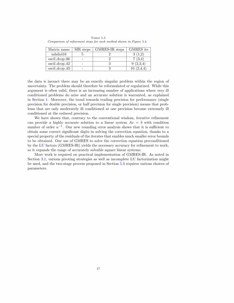
Table 5.5Comparison of refinement steps for each method shown in Figure 5.4.

Matrix name SIR steps GMRES-IR steps GMRES itsmhda416 5 2 3 (1,2)

oscil dcop 06 - 2 7 (3,4)oscil dcop 42 - 3 9 (2,3,4)oscil dcop 43 - 3 10 (2,4,4)

the data is inexact there may be an exactly singular problem within the region ofuncertainty. The problem should therefore be reformulated or regularized. While thisargument is often valid, there is an increasing number of applications where very illconditioned problems do arise and an accurate solution is warranted, as explainedin Section 1. Moreover, the trend towards trading precision for performance (singleprecision for double precision, or half precision for single precision) means that prob-lems that are only moderately ill conditioned at one precision become extremely illconditioned at the reduced precision.

We have shown that, contrary to the conventional wisdom, iterative refinementcan provide a highly accurate solution to a linear system Ax = b with conditionnumber of order u−1. Our new rounding error analysis shows that it is sufficient toobtain some correct significant digits in solving the correction equation, thanks to aspecial property of the residuals of the iterates that enables much smaller error boundsto be obtained. Our use of GMRES to solve the correction equation preconditionedby the LU factors (GMRES-IR) yields the necessary accuracy for refinement to work,so it expands the range of accurately solvable square linear systems.

More work is required on practical implementation of GMRES-IR. As noted inSection 3.1, various pivoting strategies as well as incomplete LU factorization mightbe used, and the two-stage process proposed in Section 5.3 requires various choices ofparameters.

17

0 5 10 15re-nement step i

10-10

10-5

100

105

ei

0 5 10 15re-nement step i

10-10

10-5

100

7(1)i

0 5 10 15re-nement step i

10-10

10-5

100

3iu

Test 1: gallery(’randsvd’,100,1e7,3)

0 5 10 15re-nement step i

10-10

10-5

100

105

ei

0 5 10 15re-nement step i

10-10

10-5

100

7(1)i

0 5 10 15re-nement step i

10-10

10-5

100

3iu

Test 2: gallery(’randsvd’,100,1e8,3)

0 5 10 15re-nement step i

10-10

10-5

100

105

ei

0 5 10 15re-nement step i

10-10

10-5

100

7(1)i

0 5 10 15re-nement step i

10-10

10-5

100

3iu

Test 3: gallery(’randsvd’,100,1e9,3)

0 5 10 15re-nement step i

10-10

10-5

100

105

ei

0 5 10 15re-nement step i

10-10

10-5

100

7(1)i

0 5 10 15re-nement step i

10-10

10-5

100

3iu

Test 4: gallery(’randsvd’,100,1e10,3)

Fig. 5.1. Relative error ei = ‖x − xi‖∞/‖x‖∞ (left), µ(∞)i (middle), and θiu (right) versus

refinement step i for tests generated using the MATLAB function randsvd, with condition numbers(from top to bottom) 107, 108, 109, and 1010. Here u = 2−24 (single precision) and u = 2−53 (doubleprecision). Red circles correspond to standard iterative refinement and blue squares correspond toGMRES-IR.

18

0 5 10 15re-nement step i

10-15

10-10

10-5

100

ei

0 5 10 15re-nement step i

10-15

10-10

10-5

100

7(1)i

0 5 10 15re-nement step i

10-15

10-10

10-5

100

3iu

Test 1: gallery(’randsvd’,100,1e15,3)

0 5 10 15re-nement step i

10-15

10-10

10-5

100

ei

0 5 10 15re-nement step i

10-15

10-10

10-5

100

7(1)i

0 5 10 15re-nement step i

10-15

10-10

10-5

100

3iu

Test 2: gallery(’randsvd’,100,1e16,3)

0 5 10 15re-nement step i

10-15

10-10

10-5

100

ei

0 5 10 15re-nement step i

10-15

10-10

10-5

100

7(1)i

0 5 10 15re-nement step i

10-15

10-10

10-5

100

3iu

Test 3: gallery(’randsvd’,100,1e17,3)

0 5 10 15re-nement step i

10-15

10-10

10-5

100

ei

0 5 10 15re-nement step i

10-15

10-10

10-5

100

7(1)i

0 5 10 15re-nement step i

10-15

10-10

10-5

100

3iu

Test 4: gallery(’randsvd’,100,1e18,3)

Fig. 5.2. Relative error ei = ‖x − xi‖∞/‖x‖∞ (left), µ(∞)i (middle), and θiu (right) versus

refinement step i for tests generated using the MATLAB function randsvd, with condition numbers(from top to bottom) 1015, 1016, 1017, and 1018. Here u = 2−53 (double precision) and u = 2−113

(quadruple precision). Red circles correspond to standard iterative refinement and blue squarescorrespond to GMRES-IR.

19

0 5 10 15re-nement step i

10-10

10-5

100

ei

0 5 10 15re-nement step i

10-10

10-5

100

7(1)i

0 5 10 15re-nement step i

10-10

10-5

100

3iu

Test 1:radfr1

0 5 10 15re-nement step i

10-10

10-5

100

ei

0 5 10 15re-nement step i

10-10

10-5

100

7(1)i

0 5 10 15re-nement step i

10-10

10-5

100

3iu

Test 2: adder dcop 06

0 5 10 15re-nement step i

10-10

10-5

100

ei

0 5 10 15re-nement step i

10-10

10-5

100

7(1)i

0 5 10 15re-nement step i

10-10

10-5

100

3iu

Test 3: adder dcop 19

0 5 10 15re-nement step i

10-10

10-5

100

ei

0 5 10 15re-nement step i

10-10

10-5

100

7(1)i

0 5 10 15re-nement step i

10-10

10-5

100

3iu

Test 4: adder dcop 26

Fig. 5.3. Relative error ei = ‖x − xi‖∞/‖x‖∞ (left), µ(∞)i (middle), and θiu (right) versus

refinement step i for tests from the University of Florida Sparse Matrix Collection. Here u = 2−24

(single precision) and u = 2−53 (double precision). Red circles correspond to standard iterativerefinement and blue squares correspond to GMRES-IR.

20

0 5 10 15re-nement step i

10-20

10-15

10-10

10-5

100

ei

0 5 10 15re-nement step i

10-20

10-15

10-10

10-5

100

7(1)i

0 5 10 15re-nement step i

10-20

10-15

10-10

10-5

100

3iu

Test 1: mhda416

0 5 10 15re-nement step i

10-20

10-15

10-10

10-5

100

ei

0 5 10 15re-nement step i

10-20

10-15

10-10

10-5

100

7(1)i

0 5 10 15re-nement step i

10-20

10-15

10-10

10-5

100

3iu

Test 2: oscil dcop 06

0 5 10 15re-nement step i

10-20

10-15

10-10

10-5

100

ei

0 5 10 15re-nement step i

10-20

10-15

10-10

10-5

100

7(1)i

0 5 10 15re-nement step i

10-20

10-15

10-10

10-5

100

3iu

Test 3: oscil dcop 42

0 5 10 15re-nement step i

10-20

10-15

10-10

10-5

100

ei

0 5 10 15re-nement step i

10-20

10-15

10-10

10-5

100

7(1)i

0 5 10 15re-nement step i

10-20

10-15

10-10

10-5

100

3iu

Test 4: oscil dcop 43

Fig. 5.4. Relative error ei = ‖x − xi‖∞/‖x‖∞ (left), µ(∞)i (middle), and θiu (right) versus

refinement step i for tests from the University of Florida Sparse Matrix Collection. Here u = 2−53

(double precision) and u = 2−113 (quadruple precision). Red circles correspond to standard iterativerefinement and blue squares correspond to GMRES-IR.

21

REFERENCES

[1] M. Arioli and I. S. Duff. Using FGMRES to obtain backward stability in mixed precision.Electron. Trans. Numer. Anal., 33:31–44, 2009.

[2] M. Arioli, I. S. Duff, S. Gratton, and S. Pralet. A note on GMRES preconditioned by aperturbed LDLT decomposition with static pivoting. SIAM J. Sci. Comput., 29(5):2024–2044, 2007.

[3] David H. Bailey and Jonathan M. Borwein. High-precision arithmetic in mathematical physics.Mathematics, 3(2):337–367, 2015.

[4] Gleb Beliakov and Yuri Matiyasevich. A parallel algorithm for calculation of determinants andminors using arbitrary precision arithmetic. BIT, 56(1):33–50, 2015.

[5] Timothy A. Davis. University of Florida Sparse Matrix Collection. http://www.cise.ufl.edu/research/sparse/matrices.

[6] Timothy A. Davis and Yifan Hu. The University of Florida Sparse Matrix Collection. ACMTrans. Math. Software, 38(1):1:1–1:25, 2011.

[7] James Demmel, Yozo Hida, William Kahan, Xiaoye S. Li, Sonil Mukherjee, and E. Jason RiedyRiedy. Error bounds from extra-precise iterative refinement. ACM Trans. Math. Software,32(2):325–351, 2006.

[8] J. Drkosova, A. Greenbaum, M. Rozloznık, and Z. Strakos. Numerical stability of GMRES.BIT, 35:309–330, 1995.

[9] Iain S. Duff. MA57—A code for the solution of sparse symmetric definite and indefinite systems.ACM Trans. Math. Software, 30(2):118–144, 2004.

[10] Iain S. Duff and Stephane Pralet. Towards stable mixed pivoting strategies for the sequentialand parallel solution of sparse symmetric indefinite systems. SIAM J. Matrix Anal. Appl.,29(3):1007–1024, 2007.

[11] Massimiliano Ferronato, Carlo Janna, and Giorgio Pini. Parallel solution to ill-conditioned FEgeomechanical problems. International Journal for Numerical and Analytical Methods inGeomechanics, 36(4):422–437, 2012.

[12] Suyog Gupta, Ankur Agrawal, Kailash Gopalakrishnan, and Pritish Narayanan. Deep learningwith limited numerical precision. In Proceedings of the 32nd International Conferenceon Machine Learning, volume 37 of JMLR: Workshop and Conference Proceedings, 2015,pages 1737–1746.

[13] Yun He and Chris H. Q. Ding. Using accurate arithmetics to improve numerical reproducibilityand stability in parallel applications. J. Supercomputing, 18(3):259–277, 2001.

[14] Nicholas J. Higham. Iterative refinement for linear systems and LAPACK. IMA J. Numer.Anal., 17(4):495–509, 1997.

[15] Nicholas J. Higham. Accuracy and Stability of Numerical Algorithms. Second edition, Societyfor Industrial and Applied Mathematics, Philadelphia, PA, USA, 2002. xxx+680 pp. ISBN0-89871-521-0.

[16] J. D. Hogg and J. A. Scott. A fast and robust mixed-precision solver for the solution of sparsesymmetric linear systems. ACM Trans. Math. Software, 37(2):17:1–17:24, 2010.

[17] IEEE Standard for Floating-Point Arithmetic, IEEE Std 754-2008 (revision of IEEE Std 754-1985). IEEE Computer Society, New York, 2008. 58 pp. ISBN 978-0-7381-5752-8.

[18] Yuka Kobayashi and Takeshi Ogita. A fast and efficient algorithm for solving ill-conditionedlinear systems. JSIAM Letters, 7:1–4, 2015.

[19] Yuka Kobayashi and Takeshi Ogita. Accurate and efficient algorithm for solving ill-conditionedlinear systems by preconditioning methods. Nonlinear Theory and Its Applications, IEICE,7(3):374–385, 2016.

[20] Xiaoye S. Li and James W. Demmel. Making sparse Gaussian elimination scalable by staticpivoting. In Proceedings of the 1998 ACM/IEEE Conference on Supercomputing, IEEEComputer Society, Washington, DC, USA, 1998, pages 1–17. CD ROM.

[21] Ding Ma and Michael Saunders. Solving multiscale linear programs using the simplex methodin quadruple precision. In Numerical Analysis and Optimization, Mehiddin Al-Baali, LucioGrandinetti, and Anton Purnama, editors, number 134 in Springer Proceedings in Mathe-matics and , Springer-Verlag, Berlin, 2015, pages 223–235.

[22] Ding Ma, Laurence Yang, Ronan M. T. Fleming, Ines Thiele, Bernhard O. Palsson, andMichael A. Saunders. Quadruple-Precision Solution of Genome-Scale Models of Metabolismand Macromolecular Expression, May 2016. ArXiv preprint 1606.00054.

[23] Multiprecision Computing Toolbox. Advanpix, Tokyo. http://www.advanpix.com.[24] Takeshi Ogita. Accurate matrix factorization: Inverse LU and inverse QR factorizations. SIAM

J. Matrix Anal. Appl., 31(5):2477–2497, 2010.[25] Shin’ichi Oishi, Takeshi Ogita, and Siegfried M. Rump. Iterative refinement for ill-conditioned

22

linear systems. Japan J. Indust. Appl. Math., 26(2-3):465–476, 2009.[26] Christopher C. Paige, Miro Rozloznık, and Zdenek Strakos. Modified Gram-Schmidt (MGS),

least squares, and backward stability of MGS-GMRES. SIAM J. Matrix Anal. Appl., 28(1):264–284, 2006.

[27] T. N. Palmer. More reliable forecasts with less precise computations: A fast-track route tocloud-resolved weather and climate simulators? Phil. Trans. R. Soc. A, 372(2018), 2014.

[28] Siegfried M. Rump. Approximate inverses of almost singular matrices still contain useful infor-mation. Technical Report 90.1, Hamburg University of Technology, 1990.

[29] Siegfried M. Rump. Inversion of extremely ill-conditioned matrices in floating-point. JapanJournal of Industrial and Applied Mathematics, 26(2-3):249–277, 2009.

[30] Youcef Saad. A flexible inner-outer preconditioned GMRES algorithm. SIAM J. Sci. Comput.,14(2):461–469, 1993.

[31] Youcef Saad and Martin H. Schultz. GMRES: A generalized minimal residual algorithm forsolving nonsymmetric linear systems. SIAM J. Sci. Statist. Comput., 7(3):856–869, 1986.

[32] Scott A. Sarra. Radial basis function approximation methods with extended precision floatingpoint arithmetic. Engineering Analysis with Boundary Elements, 35(1):68–76, 2011.

[33] Robert D. Skeel. Iterative refinement implies numerical stability for Gaussian elimination.Math. Comp., 35(151):817–832, 1980.

[34] Kathryn Turner and Homer F. Walker. Efficient high accuracy solutions with GMRES(m).SIAM J. Sci. Statist. Comput., 13(3):815–825, 1992.

[35] Homer F. Walker. Implementation of the GMRES method using Householder transformations.SIAM J. Sci. Statist. Comput., 9(1):152–163, 1988.

[36] J. H. Wilkinson. The use of the single-precision residual in the solution of linear systems.Unpublished manuscript, 1977. 11 pp.

23