a new class of particle filters for random dynamic systems

EURASIP Journal on Applied Signal Processing 2004:15, 2278–2294c© 2004 Hindawi Publishing Corporation

A New Class of Particle Filters for Random DynamicSystems with Unknown Statistics

Joaquın MıguezDepartamento de Electronica e Sistemas, Universidade da Coruna, Facultade de Informatica, Campus de Elvina s/n,15071 A Coruna, SpainEmail: [email protected]

Monica F. BugalloDepartment of Electrical and Computer Engineering, State University of New York at Stony Brook, Stony Brook,NY 11794-2350, USAEmail: [email protected]

Petar M. DjuricDepartment of Electrical and Computer Engineering, State University of New York at Stony Brook, Stony Brook,NY 11794-2350, USAEmail: [email protected]

Received 4 May 2003; Revised 29 January 2004

In recent years, particle filtering has become a powerful tool for tracking signals and time-varying parameters of random dynamicsystems. These methods require a mathematical representation of the dynamics of the system evolution, together with assumptionsof probabilistic models. In this paper, we present a new class of particle filtering methods that do not assume explicit mathematicalforms of the probability distributions of the noise in the system. As a consequence, the proposed techniques are simpler, morerobust, and more flexible than standard particle filters. Apart from the theoretical development of specific methods in the newclass, we provide computer simulation results that demonstrate the performance of the algorithms in the problem of autonomouspositioning of a vehicle in a 2-dimensional space.

Keywords and phrases: particle filtering, dynamic systems, online estimation, stochastic optimization.

1. INTRODUCTION

Many problems in signal processing can be stated in terms ofthe estimation of an unobserved discrete-time random signalin a dynamic system of the form

xt = fx(xt−1) + ut , t = 1, 2, . . . , (1)

yt = fy(xt) + vt, t = 1, 2, . . . , (2)

where

(a) xt ∈ RLx is the signal of interest, which represents thesystem state at time t;

(b) fx : RLx → Ix ⊆ RLx is a (possibly nonlinear) statetransition function;

(c) ut ∈ RLx is the state perturbation or system noise attime t;

(d) yt ∈ RLy is the vector of observations collected at timet, which depends on the system state;

(e) fy : RLx → Iy ⊆ RLy is a (possibly nonlinear) transfor-mation of the state;

(f) vt ∈ RLy is the observation noise vector at time t, as-sumed statistically independent from the system noiseut.

Equation (1) describes the dynamics of the system state vec-tor and, hence, it is usually termed state equation or systemequation, whereas (2) is commonly referred to as observationequation or measurement equation. It is convenient to dis-tinguish the structure of the dynamic system defined by thefunctions fx and fy from the associated probabilistic model,which depends on the probability distribution of the noisesignals and the a priori distribution of the state, that is, thestatistics of x0.

We denote the a priori probability density function (pdf)of a random signal s as p(s). If the signal s is statisticallydependent on some observation z, then we write the con-ditional (or a posteriori) pdf as p(s|z). From the Bayesianpoint of view, all the information relevant for the estimation

mailto:[email protected]



A New Class of Particle Filters 2279

of the state at time t is contained in the so-called filtering pdf,that is, the a posteriori density of the system state given theobservations up to time t,

p(

xt|y1:t), (3)

where y1:t = {y1, . . . , yt}. The density (3) usually involvesa multidimensional integral which does not have a closed-form solution for an arbitrary choice of the system structureand the probabilistic model. Indeed, analytical solutions canonly be obtained for particular setups. The most classical ex-ample occurs when fx and fy are linear functions and thenoise processes are Gaussian with known parameters. Thenthe filtering pdf of xt is itself Gaussian, with mean mt andcovariance matrix Ct, which we denote as

p(

xt|y1:t) = N

(mt , Ct

), (4)

where the posterior parameters mt and Ct can be recur-sively computed, as time evolves, using the elegant algorithmknown as Kalman filter (KF) [1]. Unfortunately, the assump-tions of linearity and Gaussianity do not hold for mostreal-world problems. Although modified Kalman-like solu-tions that account for general nonlinear and non-Gaussiansettings have been proposed, including the extended KF(EKF) [2] and the unscented KF (UKF) [3], such tech-niques are based on simplifications of the system dynam-ics and suffer from severe degradation when the true dy-namic system departs from the linear and Gaussian assump-tions.

Since general analytical solutions are intractable, Baye-sian estimation in nonlinear, non-Gaussian systems mustbe addressed using numerical techniques. Deterministic ap-proaches, such as classical numerical integration procedures,turn out ineffective or too demanding except for very low-dimensional systems and, as a consequence, methods basedon the Monte Carlo methodology have progressively gainedmomentum. Monte Carlo methods are simulation-basedtechniques aimed at estimating the a posteriori pdf of thestate signal given the available observations. The pdf esti-mate consists of a random grid of weighted points in the statespace RLx . These points, usually termed particles, are MonteCarlo samples of the system state that are assigned nonnega-tive weights, which can be interpreted as probabilities of theparticles.

The collection of particles and their weights yield an em-pirical measure which approximates the continuous a poste-riori pdf of the system state [4]. The recursive update of thismeasure whenever a new observation is available is knownas particle filtering (PF). Although there are other popularMonte Carlo methods based on the idea of producing em-pirical measures with random support, for example, MarkovChain Monte Carlo (MCMC) techniques [5], PF algorithmshave recently received a lot of attention because they are par-ticularly suitable for real-time estimation. The sequential im-portance sampling (SIS) algorithm [6, 7] and the bootstrapfilter (BF) [8, 9] are the most successful members of the PFclass of methods [10]. Existing PF techniques rely on

(i) the knowledge of the probabilistic model of the dy-namic system (1)-(2), which includes the densitiesp(x0), p(ut), and p(vt),

(ii) the ability to numerically evaluate the likelihoodp(yt|xt) and to sample from the transition densityp(xt|xt−1).

Therefore, the practical performance of PF algorithms inreal-world problems heavily depends on how accurate theunderlying probabilistic model of choice is. Although thismay seem irrelevant in engineering problems where it is rel-atively straightforward to associate the observed signals withrealistic and convenient probability distributions, in manysituations, this is not the case. Many times, it is very hardto find an adequate model using the information availablein practice. In other occasions, the working models obtainedafter a lot of effort (involving, e.g., time-series analysis tech-niques) are so complicated that they render any subsequentsignal processing algorithm impractical due to its high com-plexity.

In this paper, we introduce a new PF approach to dealwith uncertainty in the probabilistic modeling of the dy-namic system (1)-(2). We start with the requirement that theultimate objective of PF is to yield an estimate of the sig-nals of interest x0:t, given the observations y1:t. If a suitableprobabilistic model is at hand, good signal estimates can becomputed from the filtering pdf (3) induced by the model,and a PF algorithm can be employed to recursively build upa random grid that approximates the posterior distribution.However, it is often possible to use signal estimation methodsthat do not explicitly rely on the a posteriori pdf, for example,blind detection in digital communications can be performedaccording to several criteria, such as the constrained mini-mization of the received signal power [11] or the constantmodulus method [12, 13]. Such approaches are very popularbecause they are based on a simple figure of merit, and thissimplicity leads to robust and easy-to-design algorithms.

The same advantages in robustness and easy design canbe gained in PF whenever a complex (yet possibly notstrongly tied to physical reality) probabilistic model can besubstituted by a simpler reference for signal estimation. Con-trary to initial intuition, estimation techniques based onad hoc, heuristic, or, simply, alternative references, differ-ent from the state posterior distribution, are not precludedby the use of the PF methodology. It is important to real-ize that the procedure for sequential build-up of the ran-dom grid is not tied to the concept of a posteriori pdf. Wewill show that, by simply specifying a stochastic mechanismfor generating particles, the PF methodology can be success-fully used to build an approximation of any function of thesystem state that admits a recursive decomposition. Specif-ically, we propose a new family of PF algorithms in whichthe statistical reference of the a posteriori state pdf is sub-stituted by a user-defined cost function that measures thequality of the state signal estimates according to the avail-able observations. Hence, methods within the new class aretermed cost-reference particle filters (CRPFs), in contrastto conventional statistical-reference particle filters (SRPFs).

2280 EURASIP Journal on Applied Signal Processing

As long as a recursive decomposition of the cost function isfound, a PF algorithm, similar to the SIS and bootstrap meth-ods, can be used to construct a random-grid approximationof the cost function in the vicinity of its minima. For this rea-son, CRPFs yield local representations of the cost functionspecifically built to facilitate the computation of minimum-cost estimates of the state signal.

The remainder of this paper is organized as follows.The fundamentals of the CRPF family are introduced inSection 2. This includes three basic building blocks: the costand risk functions, which provide a measure of the quality ofthe particles, and the stochastic mechanism for particle gen-eration and sequential update of the random grid. Since theusual tools for PF algorithm design (e.g., proposal distribu-tions, auxiliary variables, etc.) do not necessarily extend tothe new framework, this section also contains a discussion ondesign issues. In particular, we identify the factors on whichthe choice of the cost and risk functions will usually depend,and derive consequent design guidelines, including a usefulchoice of parameters that leads to a simple interpretation ofthe algorithm and its connection with the theory of stochas-tic approximation (SA) [14].

Due to the change in the reference, convergence resultsregarding SRPFs are not valid for CRPFs. Section 3 is devotedto the problem of identifying sufficient conditions for asymp-totically optimal propagation (AOP) of particles. The stochas-tic procedure for drawing new samples of the state signal andpropagating the existing particles using the new samples isthe key for the convergence of the algorithm. We term thisparticle propagation step as asymptotically optimal when theincrement in the average cost of the particles in the filter afterpropagation is minimal. A set of sufficient conditions for op-timal propagation, related to the properties of the samplingand weighting methods, is provided.

Section 4 is devoted to the discussion of resampling in thenew family of PF techniques. We argue that the objective ofthis important algorithmic step is different from its usual rolein conventional PF algorithms, and exploit this differenceto propose a local resampling scheme suitable for a straight-forward implementation using parallel VLSI hardware (notethat resampling is a major bottleneck for the parallel imple-mentation of PF methods [15]).

Computer simulation results that illustrate the validityof our approach are presented in Section 5. In particular, wetackle the problem of positioning a vehicle that moves alonga 2-dimensional space. An instance of the proposed CRPFclass of methods that employs a simple cost function is com-pared with the standard auxiliary BF [9] technique. Finally,Section 6 contains conclusions.

2. COST-REFERENCE PARTICLE FILTERING

The basics of the new family of PF methods are introducedin this section. We start with a general description of theCRPF technique, where key concepts, namely, the cost andrisk functions, particle propagation, and particle selection,are introduced. The second part of the section is devoted topractical design issues. We suggest guidelines for the design

of CRPFs and propose a simple choice of the algorithm pa-rameters that lead to a straightforward interpretation of theCRPF technique.

2.1. Sequential algorithm

The ultimate aim of the method is the online estimation ofthe sequence of system states from the available observations,that is, we intend to estimate xt|y1:t, t = 0, 1, 2, . . . , accord-ing to some reference function that yields a quantitative mea-sure of quality. In particular, we propose the use of a real costfunction with a recursive additive structure, that is,

C(

x0:t|y1:t, λ) = λC

(x0:t−1|y1:t−1, λ

)+�C

(xt|yt

), (5)

where 0 < λ < 1 is a forgetting factor, �C : RLx × RLy → Ris the incremental cost function, and C(x0:t|y1:t, λ) complieswith the definition

C : R(t+1)Lx ×RtLy ×R −→ R. (6)

We should remark that (5) is not the only recursive decom-position that can be employed. A straightforward alternativeis to choose a cost function which is built at time t as theconvex sum

C(

x0:t|y1:t, λ) = λC

(x0:t−1|y1:t−1, λ

)+ (1− λ)�C(xt|yt).

(7)

This form of cost function is perfectly valid for the defini-tion and construction of CRPFs and choosing it would notaffect (or would affect trivially) the arguments presented inthe rest of this paper, including the asymptotic convergenceresults in Section 3. However, we will constrain ourselves tothe familiar form of (5) for simplicity.

A high value of C(x0:t|y1:t, λ) means that the state se-quence x0:t is not a good estimate given the sequence of ob-servations y1:t, while a low value of C(x0:t|y1:t, λ) indicatesthat x0:t is close to the true state signal. The sequence x0:t issaid to have a high cost, in the former case, or a low cost, inthe latter case. Particularly notice the recursive structure in(5), where the cost of a sequence up to time t − 1 can be up-dated by solely looking at the state and observation vectorsat time t, xt , and yt , respectively, which are used to computethe cost increment�C(xt|yt). The forgetting factor λ avoidsattributing an excessive weight to old observations when along series of data are collected, hence allowing for potentialadaptivity.

We also introduce a one-step risk function of the form

R : RLx ×RLy −→ R,

xt−1, yt �R(

xt−1|yt) (8)

that measures the adequacy of the state at time t−1 given thenew observation yt. It is convenient to view the risk functionR(xt−1|yt) as a prediction of the cost increment �C(xt|yt)that can be obtained before xt is actually propagated. Hence,a natural choice of the risk function is

R(

xt−1∣∣yt) = �C

(fx(

xt−1)∣∣yt

). (9)


The proposed estimation technique proceeds sequen-tially in a similar manner as the BF. Given a set of Mstate samples and associated costs up to time t, that is, theweighted-particle set (wps)

Ξt ={

x(i)t , C(i)

t

}Mi=1, (10)

where C(i)t = C(x(i)

0:t|y1:t, λ), the grid of state trajectories israndomly propagated when yt+1 is observed in order to buildan updated wps Ξt+1. The state and observation signals arethose described in the dynamic system (1)-(2). We only addthe following mild assumptions:

(1) the initial state is known to lie in a bounded intervalIx0 ⊂ RLx ;

(2) the system and observation noise are both zero mean.

Assumption (1) is needed to ensure that we initially draw aset of samples that is not infinitely far from the true state x0.Notice that this is a structural assumption, not a probabilis-tic one. Assumption (2) is made for the sake of simplicitybecause zero-mean noise is the rule in most systems.

The sequential CRPF algorithm based on the structureof system (1)-(2), the definitions of cost and risk functionsgiven by (5) and (8), respectively, and assumptions (1) and(2), is described below.

(1) Time t = 0 (initialization). DrawM particles from theuniform distribution in the interval Ix0 ,

x(i)0 ∼U

(Ix0

), (11)

and assign them a zero cost. The initial wps

Ξ0 ={

x(i)0 , C(i)

0 = 0}Mi=1 (12)

is obtained.(2) Time t+1 (selection of the most promising trajectories).

The goal of the selection step is to replicate those particleswith a low cost while high-cost particles are discarded. Asusual in PF methods, selection is implemented by a resam-pling procedure [7]. We point out that, differently from thestandard BF, resampling in CRPFs does not produce equallyweighted particles. Instead, each particle preserves its owncost. Notice that the equal weighting of resampled particlesin standard PF algorithms comes from the use of a statisti-cal reference. In CRPF, preserving the particle costs after re-sampling actually shifts the random grid representation ofthe cost function toward its local minima. Such a behavioris sound, as we are interested in minimum cost signal esti-mates. Further issues related to resampling are discussed inSection 4.

For i = 1, 2, . . . ,M, compute the one-step risk of particlei and let

R(i)t+1 = λC(i)

t + R(

x(i)t |yt+1

)(13)

which yields a predictive cost of the trajectory x0:t accordingto the new observation yt. Define a probability mass function(pmf) of the form

π(i)t+1 ∝ µ

(R(i)

t+1

), (14)

where µ : R → [0, +∞) is a monotonically decreasing func-tion. An intermediate wps is obtained by resampling the

trajectories {x(i)t }Mi=1 according to the pmf π(i)

t+1. Specifically,

we select x(i)t = x(k)

t with probability π(k)t+1, and build the

set Ξt+1 = {x(i)t , C(i)

t }Mi=1, where C(i)t = C(k)

t if and only if

x(i)t = x(k)

t .(3) Time t + 1 (random particle propagation). Select an

arbitrary conditional pdf of the state pt+1(xt+1|xt) with theconstraint that

Ept+1(xt+1|xt)[

xt+1] = fx

(xt), (15)

where Ep(s)[·] denotes expected value with respect to the pdfin the subindex. Using the selected propagation density, drawnew particles

x(i)t+1 ∼ pt+1

(xt+1|x(i)

t

)(16)

and update the associated costs

C(i)t+1 = λC(i)

t +�C(i)t+1, (17)

where

�C(i)t+1 = �C

(x(i)t+1

∣∣yt+1)

(18)

for i = 1, 2, . . . ,M.As a result, the updated wps Ξt+1 = {x(i)

t+1, C(i)t+1}Mi=1 is ob-

tained.(4) Time t + 1 (estimation of the state). Estimation pro-

cedures are better understood if a pmf π(i)t+1, i = 1, 2, . . . ,M,

is assigned to the particles in Ξt+1. The natural way to definethis pmf is according to the particle costs, that is,

π(i)t+1 ∝ µ

(C(i)t+1

), (19)

where µ is a monotonically decreasing function.The minimum cost estimate at time t+ 1 is trivially com-

puted as

i0 = arg maxi

{π(i)t+1

},

xmin0:t+1 = x(i0)

t+1

(20)


and its physical meaning is obvious. An equally useful esti-

mate can be computed as the mean value of x(i)t+1 according to

the pmf π(i)t+1, that is,

xmeant+1 =

M∑i=1

π(i)t+1x(i)

t+1. (21)

Note that xmeant+1 can also be regarded as a minimum cost es-

timate because the particle set Ξt+1 is a random-grid localrepresentation of the cost function in the vicinity of its min-ima. In fact, estimator (21) has slight advantages over (20).

Namely, the averaging of particles according to the pmf π(i)t+1

yields an estimated state trajectory which is smoother thanthe one resulting from simply choosing the particle with theleast cost at each time step. Besides, computing the mean

of the particles under π(i)t+1 may result in an estimate with a

slightly smaller cost than the least cost particle, since xmeant+1

is obtained by interpolation of particles around the least coststate.

Sufficient conditions for the mean estimate (21) to attainan asymptotically minimum cost are given in Section 3.

We will refer to the general procedure described above asa CRPF algorithm. It is apparent that many implementationsare possible for a single problem, so in the next section, wediscuss the choice of the functions and parameters involvedin the method.

2.2. Design issues

An instance of the CRPF class of algorithms is selected bychoosing

(i) the cost function C(·|·),(ii) the risk function R(·|·),

(iii) the monotonically decreasing function µ : R → [0,+∞) that maps costs and risks into the resampling andestimation pmfs, as indicated in (14) and (19), respec-tively,

(iv) the sequence of pdfs pt+1(xt+1|xt) for particle genera-tion.

The cost and risk functions measure the quality of the par-ticles in the filter. Recall that the risk is conveniently inter-preted as a prediction of the cost of a particle, given a new ob-servation, before random propagation is actually carried out(see the selection step in Section 2.1). Therefore, the cost andthe risk should be closely related, and we suggest to chooseR(·|·) according to (9). Whenever possible, both the costand risk functions should be

(i) strictly convex in the range of values of xt, where thestate is expected to lie, in order to avoid ambiguities inthe estimators (20) and (21) as well as in the selection(resampling) step,

(ii) easy to compute in order to facilitate the practical im-plementation of the algorithm,

(iii) dependent on the complete state and observation sig-nals, that is, it should involve all the elements of xt andyt.

A simple, yet useful and physically meaningful, choice ofC(·|·, ·), R(·|·) that will be used in the numerical examplesof Section 5 is given by

C(

x0) = 0, (22)

�C(

xt∣∣yt) = ∥∥yt − fy

(xt)∥∥q, (23)

R(

xt∣∣yt+1

) = ∥∥yt+1 − fy(fx(

xt))∥∥q, (24)

where q ≥ 1 and ‖v‖ = √vTv denotes the norm of v. Given afixed and bounded sequence of observations y1:t, the optimal(minimum cost) sequence of state vectors is

xopt0:t = arg min

x0:t

{C(

x0:t∣∣y1:t, λ

)}

= arg minx0:t

{ t∑k=0

λ(t−k)�C(

xt∣∣yt)}.

(25)

We call xopt0:t optimal because it is obtained by minimization

of the continuous cost function, and it is in general differentfrom the minimum cost estimate obtained by CRPF, whichwe have denoted as xmin

0:t in Section 2.1.With the assumed choice of cost and risk functions given

by (22)–(24), the invertible observation function fy : RLx →Iy ⊆ RLy , and yt ∈ Iy , for all t ≥ 1, it is straightforward toderive a pointwise solution of the form1

xoptt = arg min

xt

{�C(

xt∣∣yt)} = f −1

y

(yt). (26)

Therefore, as the CRPF algorithm randomly selects andpropagates the sample states with the least cost, it can be un-derstood (again, under assumption of (22)–(24)) as a nu-merical stochastic method for approximately solving the setof (possibly nonlinear) equations

yt − fy(

xt) = 0, t = 1, 2, . . . . (27)

Furthermore, setting q = 1 in (23) and (24), we obtain aMonte Carlo estimate of the mean absolute deviation solu-tion of the above set of equations, while q = 2 results in astochastic optimization of the least squares type.

This interpretation of the CRPF algorithm as a methodfor numerically solving (27) allows to establish a connec-tion between the proposed methodology and the theory ofSA [14], which is briefly commented upon in Appendix A.

The function µ : R → [0, +∞) should be selected toguarantee an adequate discrimination of low-cost particlesfrom those presenting higher costs (recall that we are inter-ested in computing a local representation of the cost func-tion in the vicinity of its minima). As shown in Section 5,the choice of µ has a direct impact on the algorithm perfor-mance. Specifically, notice that the accuracy of the selectionstep is highly dependent on the ability of µ to assign largeprobability masses to lower-cost particles.

1Note, however, that additional solutions may exist at ∇x fy(x) = 0 de-pending on fy(·).


A straightforward choice of this function is

µ1(C(i)t

) = C(i)t

−1, C(i)

t ∈ R \ {0}, (28)

which is simple to compute and potentially useful in manysystems. It has a serious drawback, however, in situations

where the range of the costs, that is, maxi{C(i)t }−mini{C(i)

t },is much smaller than the average cost (1/M)

∑Mi=1 C(i)

t . Insuch scenarios, µ1 yields nearly uniform probability massesand the algorithm performance degrades. Better discrimina-tion properties can be achieved with an adequate modifica-tion of µ1, for example, with

µ2(C(i)t

) = 1(C(i)t −mink

{C(k)t

}+ δ

)β , (29)

where 0 < δ < 1 and β > 1. When compared with µ1, µ2

assigns larger masses to low-cost particles and much smallermasses to higher-cost samples. The discrimination ability ofµ2 is enhanced by reducing the value of δ (i.e., δ 0) and/orincreasing β. The relative merit of µ2 over µ1 is experimen-tally illustrated in Section 5.

The last selection to be made is the pdf for particle prop-agation, pt+1(xt+1|xt), in step 3 of the CRPF algorithm. Thetheoretical properties required for optimal propagation areexplored in Section 3. From a practical and intuitive2 pointof view, it is desirable to use easy-to-sample pdfs with a largeenough variance to avoid losing tracks of the state signal,but not too large, to prevent the generation of too dispersedparticles. A simple strategy implemented in the simulationsof Section 5 consists of using zero-mean Gaussian densitieswith adaptively selected variance. Specifically, the particle i ispropagated from time t to time t + 1 as

x(i)t+1 ∼ N

(fx(

x(i)t−1

), σ2,(i)

t ILx), (30)

where ILx is the Lx × Lx identity function and the variance

σ2,(i)t is recursively computed as

σ2,(i)t = t − 1

tσ2,(i)t−1 +

∥∥x(i)t − fx

(x(i)t−1

)∥∥2

tLx. (31)

This adaptive-variance technique has appeared useful and ef-ficient in our simulations, as illustrated in Section 5, but al-ternative approaches (including the simple choice of a fixedvariance) can also be successfully exploited.

3. CONVERGENCE OF CRPF ALGORITHMS

In this section, we assess the convergence of the proposedCRPF algorithm. In particular, we seek sufficient conditions

2Part of this intuition is confirmed by the convergence theorem inSection 3.

for AOP of the particles from time t − 1 to time t. LetΞt = {x(i)

t , C(i)t }Mi=1 be the wps computed at time t. We say

that Ξt has been obtained by AOP from Ξt−1 if and only if

limM→∞

∣∣�C(

xoptt

∣∣yt)−�Ct

∣∣ = 0 (in some sense), (32)

where xoptt is the optimal state according to (26) and

�Ct =M∑i=1

�(i)t �C(i)

t , (33)

with a pmf �(i)t ∝ µ(�C(i)

t ), is the mean incremental cost attime t. The results presented in this section prove that AOPcan be ensured by adequately choosing the propagation den-sity and function µ : R → [0,∞) that relates the cost to the

pmf ’s π(i)t and π(i)

t . Notice that π(i)t = �(i)

t when λ = 0.A corollary of the AOP convergence theorem is also es-

tablished that provides sufficient conditions for the meanstate estimate given by (21), for the case λ = 0, to be asymp-totically optimal in terms of its incremental cost.

3.1. Preliminary definitions

Some preliminary definitions are necessary before statingand proving sufficient AOP conditions. If the selectionand propagation steps of the CRPF method are consideredjointly, it turns out that, at time t, M particles are sampled as

x(i)t ∼ pM

′t (x), (34)

where M′ < ∞ denotes the number of particles available attime t − 1 and sampling the pdf pM

′t (x) amounts to resam-

pling M times in Ξt−1 = {x(i)t−1, C(i)

t−1}M′i=1 and then propagat-

ing the resulting particles and updating the costs to build the

new wps Ξt = {x(i)t , C(i)

t }Mi=1 (note that we explicitly allowM �= M′). Although other possibilities exist, for example, asdescribed in Section 4, when multinomial resampling is usedin the selection step of the CRPF algorithm, the pdf in (34) isa finite mixture of the form

pM′

t (x) =M′∑k=1

π(k)t pt

(x∣∣x(k)

t−1

). (35)

We also introduce the following notation for a ball cen-tered at x

optt with radius ε > 0:

S{

xoptt , ε

} = {x ∈ RLx :∥∥x− x

optt

∥∥ < ε}, (36)

and we write

SM{

xoptt , ε

} = {x ∈ {x(i)t

}Mi=1 :

∥∥x − xoptt

∥∥ < ε} (37)

for its discrete counterpart built from the particles in Ξt.


3.2. Convergence theorem

Lemma 1. Let {x(i)t }Mi=1 be a set of particles drawn at time t

using the propagation pdf pM′

t (x) as defined by (34), let y1:t be afixed bounded sequence of observations, and let �C(x|yt) ≥ 0be a continuous cost function, bounded in S{x

optt , ε}, with a

minimum at x = xoptt .

If the three following conditions are met:

(1) any ball with center at xoptt has a nonzero probability un-

der the propagation density, that is,

∫S{x

optt ,ε}

pM′

t (x)dx = γ > 0 ∀ε > 0, (38)

(2) the supremum of the function µ(�C(·|·)) for pointsoutside S(x

optt , ε) is a finite constant, that is,

Sout = supxt∈RLx \S(x

optt ,ε)

{µ(�C

(xt∣∣yt))}

<∞, (39)

(3) the supremum of the function µ(�C(·|·)) for points in-side SM(x

optt , ε) converges to infinity faster than the iden-

tity function, that is,

limM→∞

M

Sin= 0, (40)

where

Sin = supxt∈SM(x

optt ,ε)

{µ(�C

(xt∣∣yt))}

, (41)

then the set function µt : A ⊆ {x(i)t }Mi=1 → [0,∞) defined as

µt(A ⊆ {x(i)

t

}Mi=1

) = ∑x∈A

µ(�C

(x∣∣yt))

(42)

is an infinite discrete measure (see definition in, e.g., [16]) thatsatisfies

limM→∞

Pr

[1− µt

(SM(

xoptt , ε

))µt({

x(i)t

}Mi=1

) ≥ δ

]= 0 ∀δ > 0, (43)

where Pr[·] denotes probability, that is,

limM→∞

µt(SM(

xoptt , ε

))µt({

x(i)t

}Mi=1

) = 1 (i.p.), (44)

where i.p. stands for “in probability.”

See Appendix B for a proof.

Theorem 1. If conditions (38), (39), and (40) in Lemma 1hold true, then the mean incremental cost at time t,

�Ct =M∑i=1

�(i)t �C

(x(i)t

∣∣yt), (45)

converges to the minimal incremental cost as M →∞,

limM→∞

∣∣�C(

xoptt

∣∣yt)−�Ct

∣∣ = 0 (i.p.). (46)

See Appendix C for a proof.Finally, an interesting corollary that justifies the use of the

mean estimate (21) can be easily derived from Lemma 1 andTheorem 1.

Corollary 1. Assuming (38), (39), and (40) in Lemma 1, andforgetting factor λ = 0, the mean cost estimate is asymptoticallyoptimal, that is,

limM→∞

∣∣�C(

xmeant

∣∣yt)−�Ct

(x

optt |yt

)∣∣ = 0 (i.p.), (47)

where

xmeant =

M∑i=1

π(i)t x(i)

t . (48)

See Appendix D for a proof.

3.3. Discussion

Theorem 1 states that conditions (38)–(40) are sufficient toachieve AOP (i.p.). The validity of this result clearly dependson the existence of a propagation pdf, pM

′t [·], and a measure

µt with good properties in order to meet the required condi-tions.

It is impossible to guarantee that condition (38) holdstrue in general, as the value of x

optt is a priori unknown, but

if the number of particles is large enough and they are evenlydistributed on the state space, it is reasonable to expect thatthe region around x

optt has a nonzero probability. Intuitively,

if the wps is locked to the system state at time t− 1, using thesystem dynamics to propagate the particles to time t shouldkeep the filtering algorithm locked to the state trajectory. In-deed, our computer simulation experiments give evidencethat the propagation pdf is not a critical weakness, and theproposed sequence of Gaussian densities given by (30) and(31) yields a remarkably good performance.

Conditions (39) and (40) are related to the choice of µor, equivalently, the measure µt. For the proposed cost modelgiven by (22) and (23), it is simple to show that condition(39) holds true, both for µ = µ1 and µ = µ2, as defined in (28)and (29), respectively. The analysis of condition (40) is moredemanding and will not be addressed here. An educated in-tuition, also supported by the computer simulation results inSection 5, points in the direction of selecting µ = µ2 with asmall enough value of δ.


PE 1

PE 6PE 2

PE 3

PE 4

PE 5

Figure 1: M = 6 processors in a ring configuration for parallel im-plementation of the local resampling algorithm.

4. RESAMPLING AND PARALLEL IMPLEMENTATION

Resampling is an indispensable algorithmic component insequential methods for statistical reference PF, which, oth-erwise, suffer from weight degeneracy and do not convergeto useful solutions [4, 7, 15]. However, resampling also be-comes a major obstacle for efficient implementation of PFalgorithms in parallel VLSI hardware devices because it cre-ates full data dependencies among processing units [15]. Al-though some promising methods have been recently pro-posed [15, 17], parallelization of resampling algorithms re-mains an open problem.

The selection step in CRPFs (see Section 2.1) is much lessrestrictive than resampling in conventional SRPFs. Specifi-cally, while resampling methods in SRPFs must ensure thatthe probability distribution of the resampled population isan unbiased and unweighted approximation of the originaldistribution of the particles [4], selection in CRPFs is onlyaimed at ensuring that the particles are close to the locationsthat produce cost function minima. We have found evidenceof state estimates obtained by CRPF being better when therandom grid of particles comprises small regions of the statespace around these minima. Therefore, selection algorithmscan be devised with the only and mild constraint that they donot increase the average cost of particles.

Now we briefly describe a simple resampling techniquefor CRPFs that lends itself to a straightforward paralleliza-tion. Figure 1 shows an array of independent processors con-nected in a ring configuration. We assume, for simplicity,that the number of processors is equal to the number ofparticles M, although the algorithm is easily generalized toa smaller number of processing elements (PEs). The ith PE

(PEi) contains the triple {x(i)t , C(i)

t , R(i)t+1} in its memory. The

proposed local resampling technique proceeds in two steps.

(i) PEi transmits {x(i)t , C(i)

t , R(i)t+1} to PEi+1 and PEi−1

and receives the corresponding information from itsneighbors. This communication step can be typicallycarried out in a single cycle and, when complete, PEicontains three particles {x(k)

t , C(k)t , R(k)

t+1}i+1k=i−1.

(ii) Each PE draws a single particle with probabilities ac-cording to the risks, that is, for the ith PE:

x(i)t = x(k)

t , C(i)t = C(k)

t , k ∈ {i− 1, i, i + 1}, (49)

with probability π(k)t = µ(R(k)

t+1)/∑i+1

l=i−1 µ(R(k)t+1).

Note that, in two simple steps, the algorithm stochasti-cally selects those particles with smaller risks. It is appar-ent that the method lends easily to parallelization, with verylimited communication requirements. The term local resam-pling comes from the observation that low-risk particles areonly locally spread by the method, that is, a PE containing ahigh-risk particle can only get a low-risk sample from its twoneighbors.

5. COMPUTER SIMULATIONS

In this section, we present computer simulations that illus-trate the validity of our approach. We have considered theproblem of autonomous positioning of a vehicle movingalong a 2-dimensional space. The vehicle is assumed to havemeans to estimate its current speed every Ts seconds and italso measures, with the same frequency, the power of threeradio signals emitted from known locations and with knownattenuation coefficients. This information can be used by aparticle filter to estimate the actual vehicle position.

Following [18], we model the positioning problem by thestate-space system

(i) state equation:

xt = Gxxt−1 + Gvvt + Guut ; (50)

(ii) observation equation:

yi,t = 10 log10

(Pi,0∥∥ri − xt

∥∥αi)

+wi,t, (51)

where xt ∈ R2 indicates the position of the vehicle in the2-dimensional reference set, Gx = I2 and Gv = Gu = TsI2

are known transition matrices, vt ∈ R2 is the observablevehicle speed, which is assumed constant during the in-terval ((t − 1)Ts, tTs), and ut is a noise process that ac-counts for measurement errors of the speed. The vector yt =[y1,t, y2,t, y3,t]T collects the received power from three emit-ters located at known reference locations ri ∈ R2, i = 1, 2, 3,that transmit their signals with initial power Pi,0 through afading channel with attenuation coefficient αi, and, finally,wt = [w1,t,w2,t,w3,t]T is the observation noise. Each timestep represents Ts seconds, the position vectors xt and ri haveunits of meters (m), the speed is given in m/s, and the re-ceived power is measured in dB. The initial vehicle positionx0 is drawn from a standard 2-dimensional Gaussian distri-bution, that is, x0 ∼ N (0, I2).

We have applied the proposed CRPF methodology forsolving the positioning problem and, for comparison andbenchmarking purposes, we have also implemented the pop-ular auxiliary BF [9], which has an algorithmic structure (re-sampling, importance sampling, and state estimation) very


Parameters. For all i,λ = 0.95; q = 1, 2; δ = 0.01; β = 2; M = 50; σ2,(i)

0 = 10.Initialization. For i = 1, . . . ,M,

x(i)0 ∼U(−8, +8),

C(i)0 = 0.

Recursive update. For i = 1, . . . ,M,

R(i)t+1 = λC(i)

t + ‖yt+1 − fy(Gxx(i)t + Gvvt+1)‖q.

Multinomial selection (resampling).

pmf : π(i)t+1 =

(R(i)t+1)−1∑M

l=1(R(l)t+1)−1

(function µ1),

(R(i)t+1 −min j∈{1,...,M} R

( j)t+1 + δ)−β∑M

l=1(R(l)t+1 −min j∈{1,...,M} R

( j)t+1 + δ)−β

(function µ2).

Selection. (x(i)t , C(i)

t ) = (x(k)t , C(k)

t ), k ∈ {1, . . . ,M}, with probability π(k)t+1.

Variance update.

t ≤ 10: σ2,(i)t+1 = σ2,(i)

t ,

t > 10: σ2,(i)t = t − 1

tσ2,(i)t−1 +

‖x(i)t − fx(x(i)

t−1)‖2

tLx.

Let x(i)t+1 ∼ pt+1(xt+1|x(i)

t ), where

Ept+1(xt+1|x(i)

t )[xt+1] = fx(x(i)

t ),

Covpt+1(xt+1|x(i)

t )[xt+1] = σ2,(i)

t+1 I2,

x(i)0:t+1 = {x(i)

0:t , x(i)t+1},

C(i)t+1 = λC(i)

t + ‖yt+1 − fy(x(i)t+1)‖q.

State estimation.

π(i)t ∝ µ1(C(i)

t ) or π(i)t ∝ µ2(C(i)

t ),

xmeant =

M∑i=1

π(i)t x

(i)t .

Algorithm 1: CRPF algorithm with multinomial resampling for the 2-dimensional positioning problem.

similar to the proposed CRPF family. Algorithm 1 summa-rizes the details of the CRPF algorithm with multinomial se-lection, including the alternatives in the choice of function µ.The selection step can be substituted by the local resamplingprocedure shown in Algorithm 2. A pseudocode for the aux-iliary BF is also provided in Algorithm 3.

In the following subsections, we describe different com-puter experiments that were carried out using synthetic datagenerated according to model (50)-(51). Two types of plotsare presented, both for CRPF and BF algorithms. Vehicle tra-jectories in the 2-dimensional space, resulting from a singlesimulation of the dynamic system, are shown to illustrate theability of the algorithms to remain locked to the state trajec-tory. We chose the mean absolute deviation as a performancefigure of merit. It was measured between the true vehicle tra-jectory in R2 and the trajectory estimated by the particle fil-ters and its unit was meter. All mean-deviation plots wereobtained by averaging 50 independent simulations. Both theBF and the CRPF type of algorithms were run with M = 50particles.

5.1. Mixture Gaussian noise processes

In the first experiment, we modeled the system and observa-tion noise processes ut and wt, respectively, as independent

and temporally white, with the mixture Gaussian pdfs:

ut ∼ 0.3N(

0,√

0.2I2)

+ 0.4N(

0, I2)

+ 0.3N(

0,√

10I2),

wl,t ∼ 0.3N (0, 0.2) + 0.4N (0, 1)

+ 0.3N (0, 10), l = 1, 2, 3.

(52)

In Figure 2, we compare the auxiliary BF with perfect knowl-edge of the noise distributions, and several CRPF algorithmsthat use the cost and risk functions proposed in Section 2.2(see (22)–(24)). For all CRPF methods, the forgetting factorwas λ = 0.95, but we ran algorithms with different values ofq, q = 1, 2, and functions µ1 and µ2 (see (28) and (29)). Forthe latter function µ2, we set δ = 0.01 and β = 2. The prop-agation mechanism for the CRPF methods consisted of thesequence of Gaussian densities given by (30) and (31), with

initial value σ2,(i)0 = 10 for all i.

Figure 2a shows the system trajectory in a single run andthe estimates corresponding to the BF and CRPF algorithms.The trajectory started in an unknown position close to (0, 0)and evolved for one hour, with sampling period Ts = 2 sec-onds. It is apparent that all the algorithms remained lockedto the vehicle position during the whole simulation interval.


Local selection (resampling) at the ith PE.

For k = i− 1, i, i + 1, π(k)t+1 =

(R(k)

t+1

)−1

∑i+1l=i−1

(R(l)

t+1

)−1

(µ1),

(R(k)

t+1 −min j∈{i−1,i,i+1} R( j)t+1 + δ

)−β∑i+1

l=i−1

(R(l)

t+1 −min j∈{i−1,i,i+1} R( j)t+1 + δ

)−β (µ2).

Selection. (x(i)t , C(i)

t ) = (x(l)t , C(l)

t ), l ∈ {i− 1, i, i + 1}, with probability π(l)t+1.

Algorithm 2: Local resampling for the CRPF algorithm.

Initialization. For i = 1, . . . ,M,

x(i)0 ∼ N (0, I2),

w(i)0 = 1

M.

Recursive update.For t = 1, . . . ,K ,

For i = 1, . . . ,M,x(i)t = fx(x(i)

t−1),

κi = k, with probability p(yt|x(k)t )w(k)

t−1,

x(i)t ∼ p[xt|x(κi)

t−1].

Weight update. w(i)t = p(yt|x(i)

t )

p(yt|x(κi)t )

.

Weight normalization. w(i)t = w(i)

t∑Mk=1 w

(k)t

.

Algorithm 3: Auxiliary BF for the 2-dimensional positioningproblem.

The latter observation is confirmed by the mean absolutedeviation plot in Figure 2b. The deviation signal was com-puted as

et = 150

12

50∑j=1

∣∣∣x1,t, j − xest1,t, j

∣∣∣ +∣∣∣x2,t, j − xest

2,t, j

∣∣∣, (53)

where j is the simulation number, xt, j = [x1,t, j , x2,t, j]T is thetrue position at time t, and xest

t, j = [xest1,t, j , x

est2,t, j]

T is the cor-responding estimate obtained with the particle filter. We ob-serve that the CRPF algorithms with µ2 attained the lowestdeviation and outperformed the auxiliary BF. Although it isnot shown here, the auxiliary BF improved its performanceas the sampling period was decreased,3 and achieved a lowerdeviation than the CRPFs for Ts ≤ 0.5 second. The reasonis that, as Ts decreases, the correlation of the states increasesdue to the variation of Gu, and the BF exploits this statisticalinformation better. Therefore, we can conclude that the BFcan be more accurate when strong statistical information isavailable, and that the proposed CRPFs are more robust and

3Obviously, the BF will also deliver a better performance as the numberof particles M grows. In fact, it can be shown [4] that the estimate of theposteriori pdf and its moments obtained from the BF converge uniformlyto the true density and the true values of the moments. This means that, asM → ∞, the state estimates given by the BF become optimal (in the meansquare error sense) and that for large M, the BF will outperform the CRPFalgorithm.

steadily attain a good performance for a wider range of sce-narios. This conclusion is easily confirmed with the remain-ing experiments presented in this section.

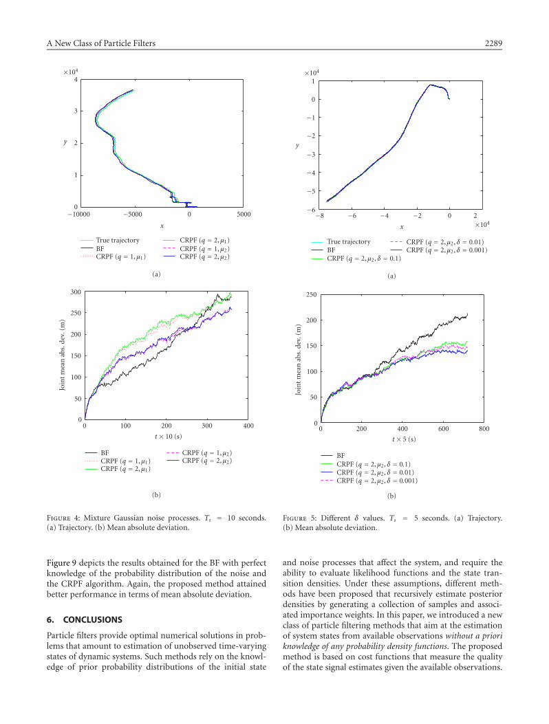
Figures 3 and 4 show the trajectories and the mean ab-solute deviations for the BF and CRPF algorithms when thesampling period was increased to Ts = 5 seconds and Ts = 10seconds, respectively. Note that increasing Ts also increasesthe speed measurement error. As before, the CRPF tech-niques with µ2 outperformed the BF in the long term.

Because of its better performance, we also checked thebehavior of the CRPF method that uses µ2 for different val-ues of parameter δ. Figure 5a shows the true position and theestimates obtained using three different values of δ, namely,0.1, 0.01, and 0.001, with fixed β = 2. All the algorithms ap-pear to perform similarly for the considered range of values.This is confirmed with the results presented in Figure 5b interms of the mean absolute deviation. They also illustrate therobustness and stability of the method.

In the following, unless it is stated differently, the CRPFalgorithm was always implemented with µ2 and parametersq = 2, δ = 0.01, and β = 2. The sampling period was alsofixed and was Ts = 5 seconds.

5.2. Mixture Gaussian system and observationnoise—Gaussian BF

Figure 6 shows the results (trajectory and mean deviation)obtained with the same system and observation noise distri-butions as in Section 5.1 when the auxiliary BF (labeled as BF(Gaussian)) is mismatched with the dynamical system andmodels the noise processes with Gaussian densities:

p[ut] = N (0,√

0.2I2),

p[wl,t] = N (0, 0.2), l = 1, 2, 3.(54)

It is apparent that the use of the correct statistical infor-mation is critical for the bootstrap algorithm (in the figure,we also plotted the result obtained when the BF used the truemixture Gaussian density—labeled as BF (M-Gaussian)).Note that the CRPF algorithm also drew the state particlesfrom a Gaussian sequence of densities (see Section 2.2), butit attained a superior performance compared to the BF.

5.3. Local versus multinomial resampling

We have verified the performance of the CRPF that uses thenew resampling scheme proposed in Section 4. The results


10−1−2−3−4×104

x

0

1

2

3

4×104

y

True trajectoryBFCRPF (q = 1,µ1)

CRPF (q = 2,µ1)CRPF (q = 1,µ2)CRPF (q = 2,µ2)

(a)

2000150010005000

t × 2 (s)

0

50

100

150

200

Join

tm

ean

abs.

dev.

(m)

BFCRPF (q = 1,µ1)CRPF (q = 2,µ1)

CRPF (q = 1,µ2)CRPF (q = 2,µ2)

(b)

Figure 2: Mixture Gaussian noise processes. Ts = 2 seconds. (a)Trajectory. (b) Mean absolute deviation.

can be observed in Figure 7. The CRPF with local resamplingshows approximately the same performance as the BF withperfect knowledge of the noise statistics. Although it presentsa slight degradation with respect to the CRPF with multi-nomial resampling, the feasibility of a simple parallel imple-mentation makes the local resampling method extremely ap-pealing.

5.4. Different estimation criteria

Figure 8 compares the trajectory and mean deviation oftwo CRPF algorithms that used different criteria to obtainthe estimates of the state: the minimum cost estimate xmin

t

20−2−4−6×104

x

0

2

4

6

8

×104

y



(a)

8006004002000

t × 5 (s)

0

50

100

150

200

250Jo

int

mea

nab

s.de

v.(m

)



(b)

Figure 3: Mixture Gaussian noise processes. Ts = 5 seconds. (a)Trajectory. (b) Mean absolute deviation.

(see (20)) and the mean cost estimate xmeant (see (21)). It is

clear that both algorithms performed similarly and outper-formed the BF in the long term.

5.5. Laplacian noise

Finally, we have repeated our experiment by modeling thenoises using Laplacian distributions, that is,

p[ut] = L(

0,√

0.5I2) = 1

0.5e−|ut|/0.5,

p[wl,t

] = 0.3L(0, 0.5) = 10.5

e−|wl,t|/0.5, l = 1, 2, 3.(55)


50000−5000−10000

x

0

1

2

3

4×104

y



(a)

4003002001000

t × 10 (s)

0

50

100

150

200

250

300

Join

tm

ean

abs.

dev.

(m)



(b)

Figure 4: Mixture Gaussian noise processes. Ts = 10 seconds.(a) Trajectory. (b) Mean absolute deviation.

Figure 9 depicts the results obtained for the BF with perfectknowledge of the probability distribution of the noise andthe CRPF algorithm. Again, the proposed method attainedbetter performance in terms of mean absolute deviation.

6. CONCLUSIONS

Particle filters provide optimal numerical solutions in prob-lems that amount to estimation of unobserved time-varyingstates of dynamic systems. Such methods rely on the knowl-edge of prior probability distributions of the initial state

20−2−4−6−8×104

x

−6

−5

−4

−3

−2

−1

0

1×104

y

True trajectoryBFCRPF (q = 2,µ2, δ = 0.1)

CRPF (q = 2,µ2, δ = 0.01)CRPF (q = 2,µ2, δ = 0.001)

(a)

8006004002000

t × 5 (s)

0

50

100

150

200

250Jo

int

mea

nab

s.de

v.(m

)

BFCRPF (q = 2,µ2, δ = 0.1)CRPF (q = 2,µ2, δ = 0.01)CRPF (q = 2,µ2, δ = 0.001)

(b)

Figure 5: Different δ values. Ts = 5 seconds. (a) Trajectory.(b) Mean absolute deviation.

and noise processes that affect the system, and require theability to evaluate likelihood functions and the state tran-sition densities. Under these assumptions, different meth-ods have been proposed that recursively estimate posteriordensities by generating a collection of samples and associ-ated importance weights. In this paper, we introduced a newclass of particle filtering methods that aim at the estimationof system states from available observations without a prioriknowledge of any probability density functions. The proposedmethod is based on cost functions that measure the qualityof the state signal estimates given the available observations.


151050−5×104

x

−5

0

5

10

15

20×103

y

True trajectoryBF (M-Gaussian)BF (Gaussian)CRPF (q = 2,µ2)

(a)

8006004002000

t × 5 (s)

0

50

100

150

200

250

300

350

Join

tm

ean

abs.

dev.

(m)

BF (M-Gaussian)BF (Gaussian)CRPF (q = 2,µ2)

(b)

Figure 6: Mixture Gaussian system and observation noise—Gaussian BF. Ts = 5 seconds. (a) Trajectory. (b) Mean absolute de-viation.

Since they do not assume explicit probabilistic models for thedynamic system, the proposed techniques, which have beentermed CRPFs, are more robust than standard particle fil-ters in problems where there is uncertainty (or a mismatchwith physical phenomena) in the probabilistic model of thedynamic system. The basic concepts related to the formu-lation and design of these new algorithms, as well as theo-retical results concerning their convergence, were provided.We also proposed a local resampling scheme that allows forsimple implementations of the CRPF techniques with paral-lel VLSI hardware. Computer simulation results illustrate the

210−1×104

x

−10

−8

−6

−4

−2

0

2×104

y

True trajectoryBFCRPF (multinomial)CRPF (local)

(a)

8006004002000

t × 5 (s)

0

50

100

150

200

250Jo

int

mea

nab

s.de

v.(m

)

BFCRPF (multinomial)CRPF (local)

(b)

Figure 7: Local versus multinomial resampling. Ts = 5 seconds.(a) Trajectory. (b) Mean absolute deviation.

robustness and the excellent performance of the proposed al-gorithms when compared to the popular auxiliary BF.

APPENDICES

A. CRPF AND STOCHASTIC APPROXIMATION

It is interesting to compare the CRPF method with the SAalgorithm. The subject of SA can be traced back to the 1951paper of Robbins and Monro [19], and a recent tutorial re-view can be found in [14].


86420−2×104

x

−2

0

2

4

6

8

10×104

y

True trajectoryBFCRPF (mean)CRPF (min)

(a)

8006004002000

t × 5 (s)

0

50

100

150

200

250

Join

tm

ean

abs.

dev.

(m)

BFCRPF (mean)CRPF (min)

(b)

Figure 8: Different estimation criteria. Ts = 5 seconds. (a) Trajec-tory. (b) Mean absolute deviation.

In a typical problem addressed by SA, an objective func-tion that has to be minimized involves expectations, for ex-ample, the minimization of E(Q(x,ψt)), where Q(·) is afunction of the unknown x and random variables ψt. Theproblem is that the distributions of the random variables areunknown and the expectation of the function cannot be an-alytically found. To make the problem tractable, one approx-imates the expectation by simply dropping the expectationoperator, and proceeding as if E(Q(x,ψt)) = Q(x,ψt). Rob-bins and Monro proposed the following scheme that solves

6420−2×104

x

−1

0

1

2

3

4

5×104

y

True trajectoryBFCRPF

(a)

8006004002000

t × 5 (s)

0

20

40

60

80

100

Join

tm

ean

abs.

dev.

(m)

BFCRPF

(b)

Figure 9: Laplacian. Ts = 5 s. (a) Trajectory. (b) Mean absolutedeviation.

for xt:

xt = xt−1 + γtQ(xt−1,ψt

), (A.1)

where γt is a sequence of positive scalars that have to satisfythe conditions

∑t γt = ∞,

∑t γ

2t <∞. In the signal processing

literature, the best known SA method is the LMS algorithm.The CRPF method also attempts to estimate the un-

known xt without probabilistic assumptions. In doing so, itactually aims at inverting the dynamic model and, therefore,


it performs SA similarly to RM though by other means.4 InCRPF, the dynamics of the state are taken into account boththrough the propagation step and by recursively solving theoptimization problem (25). Further research in CRPF fromthe perspective of SA can probably yield new and deeper in-sight of this new class of algorithms.

B. PROOF OF LEMMA 1

The proof is carried out in two steps. First, we prove the im-plication

1− δδ

Sout limM→∞

EpM′tnM

µt(SM(

xoptt , ε

)) = 0 (B.1)

⇓

limM→∞

Pr

1− µt

(SM(

xoptt , ε

))µt({

x(i)t

}Mi=1

) ≥ δ

= 0 (B.2)

for any ε, δ > 0. Then, we only need to show that (B.1) holdstrue under conditions (38)–(40) in order to complete theproof.

Straightforward manipulation of the inequality in (43)leads to the following equivalence chain that holds true forany ε, δ > 0:

limM→∞

Pr

1− µt

(SM(

xoptt , ε

))µt({

x(i)t

}Mi=1

) ≥ δ

= 0 (B.3)

�limM→∞

Pr[µt(SM(

xoptt , ε

)) ≤ (1− δ)µt({

x(i)t

}Mi=1

)] = 0 (B.4)

�

limM→∞

Pr

[µt(SM(

xoptt , ε

))

≤ 1− δδ

µt({

x(i)t

}Mi=1 \ SM

(x

optt , ε

))] = 0,

(B.5)

where we have exploited that

µt({

x(i)t

}Mi=1

) = µt(SM(

xoptt , ε

))+ µt

({x(i)t

}Mi=1 \ SM

(x

optt , ε

)).

(B.6)

Using the notation

1A(x) =1 if x ∈ A,

0 otherwise,(B.7)

4Note, however, that the notion of inversion must be understood in abroad sense, since fy may not necessarily be invertible and, even if f −1

y exists,it may happen that yt does not belong to its domain.

for the indicator function, we can write

µt({

x(i)t

}Mi=1 \ SM

(x

optt , ε

))

=M∑i=1

µ(�C

(x(i)t |yt

))1{x:‖x−x

optt ‖≥ε}

(x(i)t

)

≤ Sout

M∑i=1

1{x:|x(i)t −x

optt |≥ε}

(x(i)t

) = SoutnM ,

(B.8)

where nM is the cardinality of the discrete set {x(i)t }Mi=1 \

SM(xoptt , ε). Therefore, using (B.8) and the equivalence be-

tween (B.3) and (B.5), we arrive at the implication

limM→∞

Pr

[1− µt

(SM(

xoptt , ε

))µt({

x(i)t

}Mi=1

) ≥ δ

]= 0

⇑

limM→∞

Pr[µt(SM(

xoptt , ε

)) ≤ 1− δδ

SoutnM

]= 0.

(B.9)

Since both µ(�C(xt|yt)) ≥ 0 and (1 − δ)SoutnM/δ > 0,we can use the relationship [16, equation 4.4-5] to obtain

Pr[µt(SM(

xoptt , ε

)) ≤ 1− δδ

SoutnM

]

≤ 1− δδ

SoutEPr[nM][nM]

µt(SM(

xoptt , ε

)) ,(B.10)

where we have used the fact that the supremum Sout doesnot depend on M or nM . When jointly considered, (B.9) and(B.10) yield the implication (B.1)⇒(B.2) and we only have toshow that (B.1) holds true in order to complete the proof.

The expectation on the left-hand side of (B.1) can becomputed by resorting to assumption (38), which yields, af-ter straightforward manipulations,

limM→∞

EPr[nM][nM] = (1− γ) lim

M→∞M (i.p.). (B.11)

Substituting (B.11) into (B.1) yields

1− δδ

Sout limM→∞

EPr[nM][nM]

µt(SM(

xoptt , ε

))

= 1− δδ

Sout(1− γ) limM→∞

M

µt(SM(

xoptt , ε

))

≤ 1− δδ

Sout(1− γ) limM→∞

M

Sin= 0,

(B.12)

where the last equality is obtained from assumptions (39)and (40). The proof is complete by going back to implication(B.1)⇒(B.2).


C. PROOF OF THEOREM 1

Using Lemma 1, we obtain that the set SM(xoptt , ε) has

(asymptotically) a unit probability mass after the propaga-tion step, that is,

limM→∞

∑i:x(i)

t ∈SM(

xoptt ,ε)�(i)

t = 1 (i.p.)∀ε > 0. (C.1)

Therefore,

limM→∞

∣∣∣∣�C(

xoptt

∣∣yt)−�Ct

∣∣∣∣

= limM→∞

∣∣∣∣∣∣∣�C(

xoptt

∣∣yt)

−∑

i:x(i)t ∈SM

(x

optt ,ε)�(i)

t �C(

x(i)t |yt

)∣∣∣∣∣∣∣ (i.p.),

(C.2)

limM→∞

∣∣∣∣∣∣∣�C(

xoptt

∣∣yt)− ∑

i:x(i)t ∈SM

(x

optt ,ε)�(i)

t �C(

x(i)t

∣∣yt)∣∣∣∣∣∣∣

≤ limM→∞

∣∣∣∣∣∣�C(

xoptt

∣∣yt)

− supxt∈SM(x

optt ,ε)

{�C(

xt∣∣yt)}∣∣∣∣∣∣ (i.p.)

(C.3)

for all ε > 0.We write the upper bound on the right-hand side of

(C.3) as a function of the radius ε:

B(ε) = limM→∞

∣∣∣∣∣∣�C(

xoptt

∣∣yt)− sup

xt∈SM(xoptt ,ε)

{�C(

xt∣∣yt)}∣∣∣∣∣∣.

(C.4)

It can be easily proved that limM→∞ #SM(xoptt , ε = 1/

√M) =

∞, where # denotes the number of elements in a discrete set.Since limM→∞ 1/

√M = 0 and it is assumed that �C(·|yt) is

continuous and bounded in S(xoptt , ε) for all ε > 0, it follows

that

B(ε = 1√

M

)= 0 (i.p.) (C.5)

and, by exploiting the fact that the left-hand side of (C.2)does not depend on ε, we can readily use (C.5) to obtain

limM→∞

∣∣�C(

xoptt

∣∣yt)−�Ct

∣∣≤ B

(ε = 1√

M

)= 0 (i.p.),

(C.6)

which concludes the proof.

D. PROOF OF COROLLARY 1

When λ = 0, �(i)t = π(i)

t and, according to Lemma 1,

limM→∞

∑i:x(i)

t ∈SM(xoptt ,ε)

π(i)t = 1 (i.p.) (D.1)

for all ε > 0. Hence, we can write the mean state estimate (inthe limit M →∞) as

limM→∞

xmeant = lim

M→∞

∑x(i)t ∈SM(x

optt ,ε)

π(i)t x(i)

t (D.2)

and, therefore, the incremental cost of the mean state esti-mate can be upper bounded as

limM→∞

�C(

xmeant

∣∣yt) ≤ lim

M→∞sup

xt∈SM(xoptt ,ε)

�C(

xt|yt). (D.3)

Using inequality (D.3) and the obvious fact that�C(xoptt |yt)

is minimal by definition, we find that

limM→∞

∣∣�C(

xmeant |yt

)−�C(

xoptt |yt

)∣∣

≤ limM→∞

∣∣∣∣∣ supxt∈SM(x

optt ,ε)

�C(

xt|yt)−�C

(x

optt

∣∣yt)∣∣∣∣∣

= B(ε),(D.4)

where B(ε) is the same as defined in (C.4). Therefore, we canapply the same technique as in the proof of Theorem 1 and,taking ε = 1/

√M, we obtain

limM→∞

∣∣�C(

xmeant

∣∣yt)−�Ct

(x

optt

∣∣yt)∣∣

≤ B(ε = 1√

M

)= 0 (i.p.),

(D.5)

which concludes the proof of the corollary.

ACKNOWLEDGMENTS

This work has been supported by Ministerio de Ciencia yTecnologıa of Spain and Xunta de Galicia (Project TIC2001-0751-C04-01), and the National Science Foundation (AwardCCR-0082607). The authors wish to thank the anonymousreviewers of this paper for their very constructive commentsthat assisted us in improving the original draft. J. Mıguezwould also like to thank Professor Ricardo Cao for intellec-tually stimulating discussions which certainly contributed tothe final form of this work.


REFERENCES

[1] R. E. Kalman, “A new approach to linear filtering and predic-tion problems,” Transactions of the ASME—Journal of BasicEngineering, vol. 82, pp. 35–45, March 1960.

[2] B. D. O. Anderson and J. B. Moore, Optimal Filtering,Prentice-Hall, Englewood Cliffs, NJ, USA, 1979.

[3] S. Julier, J. Uhlmann, and H. F. Durrant-Whyte, “A newmethod for the nonlinear transformation of means and co-variances in filters and estimators,” IEEE Trans. on AutomaticControl, vol. 45, no. 3, pp. 477–482, 2000.

[4] D. Crisan and A. Doucet, “A survey of convergence resultson particle filtering methods for practitioners,” IEEE Trans.Signal Processing, vol. 50, no. 3, pp. 736–746, 2002.

[5] W. J. Fitzgerald, “Markov chain Monte Carlo methods withapplications to signal processing,” Signal Processing, vol. 81,no. 1, pp. 3–18, 2001.

[6] J. S. Liu and R. Chen, “Sequential Monte Carlo methods fordynamic systems,” Journal of the American Statistical Associa-tion, vol. 93, no. 443, pp. 1032–1044, 1998.

[7] A. Doucet, S. Godsill, and C. Andrieu, “On sequential MonteCarlo sampling methods for Bayesian filtering,” Statistics andComputing, vol. 10, no. 3, pp. 197–208, 2000.

[8] N. Gordon, D. Salmond, and A. F. M. Smith, “Novel ap-proach to nonlinear and non-Gaussian Bayesian state estima-tion,” IEE Proceedings Part F: Radar and Signal Processing, vol.140, no. 2, pp. 107–113, 1993.

[9] M. K. Pitt and N. Shephard, “Auxiliary variable based par-ticle filters,” in Sequential Monte Carlo Methods in Practice,A. Doucet, N. de Freitas, and N. Gordon, Eds., pp. 273–293,Springer, New York, NY, USA, 2001.

[10] A. Doucet, N. de Freitas, and N. Gordon, Eds., SequentialMonte Carlo Methods in Practice, Springer, New York, NY,USA, 2001.

[11] M. L. Honig, U. Madhow, and S. Verdu, “Blind adaptive mul-tiuser detection,” IEEE Transactions on Information Theory,vol. 41, no. 4, pp. 944–960, 1995.

[12] J. R. Treichler, M. G. Larimore, and J. C. Harp, “Practical blinddemodulators for high-order QAM signals,” Proceedings of theIEEE, vol. 86, no. 10, pp. 1907–1926, 1998.

[13] J. Mıguez and L. Castedo, “A linearly constrained constantmodulus approach to blind adaptive multiuser interferencesuppression,” IEEE Communications Letters, vol. 2, no. 8, pp.217–219, 1998.

[14] T. L. Lai, “Stochastic approximation,” The Annals of Statistics,vol. 31, no. 2, pp. 391–406, 2003.

[15] M. Bolic, P. M. Djuric, and S. Hong, “New resampling algo-rithms for particle filters,” in Proc. IEEE International Confer-ence on Acoustics, Speech, and Signal Processing (ICASSP ’03),vol. 2, pp. 589–592, Hong Kong, April 2003.

[16] H. Stark and J. W. Woods, Probability and Random Processeswith Applications to Signal Processing, Prentice-Hall, UpperSaddle River, NJ, USA, 3rd edition, 2002.

[17] M. Bolic, P. M. Djuric, and S. Hong, “Resampling algorithmsfor particle filters suitable for parallel VLSI implementation,”in Proc. 37th Annual Conference on Information Sciences andSystems (CISS ’03), Baltimore, Md, March 2003.

[18] F. Gustafsson, F. Gunnarsson, N. Bergman, U. Forssell, J. Jans-son, R. Karlsson, and P.-J. Nordlund, “Particle filters for posi-tioning, navigation, and tracking,” IEEE Transactions on Sig-nal Processing, vol. 50, no. 2, pp. 425–437, 2002.

[19] H. Robbins and S. Monro, “A stochastic approximationmethod,” Annals of Mathematical Statistics, vol. 22, pp. 400–407, 1951.

Joaquın Mıguez was born in Ferrol, Gali-cia, Spain, in 1974. He obtained the Licen-ciado en Informatica (M.S.) and Doctor enInformatica (Ph.D.) degrees from Universi-dade da Coruna, Spain, in 1997 and 2000,respectively. Late in 2000, he joined Depar-tamento de Electronica e Sistemas, Univer-sidade da Coruna, where he became an As-sociate Professor in July 2003. From April toDecember 2001, he was a Visiting Scholarin the Department of Electrical and Computer Engineering, StonyBrook University. His research interests are in the field of statisticalsignal processing, with emphasis on the topics of Bayesian analy-sis, sequential Monte Carlo methods, adaptive filtering, stochasticoptimization, and their applications to multiuser communications,smart antenna systems, sensor networks, target tracking, and vehi-cle positioning and navigation.

Monica F. Bugallo received the Ph.D. de-gree in computer engineering from Univer-sidade da Coruna, Spain, in 2001. From1998 to 2000, she was with the Departa-mento de Electronica e Sistemas, the Uni-versidade da Coruna, where she worked ininterference cancellation applied to mul-tiuser communication systems. In 2001, shejoined the Department of Electrical andComputer Engineering, Stony Brook Uni-versity, where she is currently an Assistant Professor, and teachescourses in digital communications and information theory. Her re-search interests lie in the area of statistical signal processing and itsapplications to different disciplines including communications andbiology.

Petar M. Djuric received his B.S. and M.S.degrees in electrical engineering from theUniversity of Belgrade in 1981 and 1986, re-spectively, and his Ph.D. degree in electricalengineering from the University of RhodeIsland in 1990. From 1981 to 1986, he was aResearch Associate with the Institute of Nu-clear Sciences, Vinca, Belgrade. Since 1990,he has been with Stony Brook University,where he is a Professor in the Department ofElectrical and Computer Engineering. He works in the area of sta-tistical signal processing, and his primary interests are in the theoryof modeling, detection, estimation, and time series analysis and itsapplication to a wide variety of disciplines including wireless com-munications and biomedicine.

a new class of particle filters for random dynamic systems

Documents