a new finite element for interface problems having … · abstract. we propose a new ﬁnite...

INTERNATIONAL JOURNAL OF c© 2017 Institute for ScientificNUMERICAL ANALYSIS AND MODELING Computing and InformationVolume 14, Number 4-5, Pages 532–549

A NEW FINITE ELEMENT FOR INTERFACE PROBLEMS

HAVING ROBIN TYPE JUMP

DO Y. KWAK, SEUNGWOO LEE, AND YUNKYONG HYON

Abstract. We propose a new finite element method for solving second order elliptic interfaceproblems whose solution has a Robin type jump along the interface. We cast the problem into anew variational form and introduce a finite element method to solve it using a uniform grid. Wemodify the P1-Crouzeix-Raviart element so that the shape functions satisfy the jump conditionsalong the interface. We note that there are cases that the Lagrange type basis can not be usedbecause of the jump in the value. Numerical experiments are provided.

Key words. Finite element, uniform grid, interface problem, Robin type jump, P1-Crouzeix-

Raviart finite element method.

1. Introduction

In recent years, there has been an extensive research towards problems involv-ing interface, (see [1, 15, 22, 37, 35, 39, 41] and references therein) and numericalmethods for such problems. A widely studied example is an elliptic problem hav-ing discontinuous coefficients, where the solution satisfies natural jump conditions[u] = 0, [β ∂u

∂n ] = 0 across the interface immersed in domain. See [14, 21, 23, 40, 41],for example. This kind of problem typically arises from diffusion phenomena ina material consisting of heterogeneous media. Other important class of prob-lem includes the time-dependent problems which may have a moving interface[24, 33, 38, 42], for instance, the incompressible Navier-Stokes equations for twofluids [19, 36] and an solid/solid or solid/fluid interaction problems [8, 9, 22]. Inmost of those examples, the primary variables, such as heat, potential, displacementand velocity, etc., or their derivatives (or flux) have certain jumps. To solve suchproblems numerically, for instance by finite element method, one usually need touse body fitted grids to get the optimal numerical results. But the grid generationis complicated and it is a time consuming job to solve the linear equation derivedfrom the body fitted grids since the matrix is unstructured.

On the other hand, a new class of finite element methods have been suggested andare shown to perform quite well for interface problems, see [14, 30, 41] and referencestherein. These methods are called immersed finite element methods (IFEMs) whichuse non fitted (say, uniform) grid for interface problems (so the interface cuts theinterior of some elements). The idea of this new method is to modify the basisfunctions so that they satisfy the interface conditions along the interface withineach element. Although the first one of these schemes was proposed for the finiteelement methods using Lagrange type P1 element having degree of freedom atvertices, the idea works well especially with Crouzeix-Raviart(CR) nonconformingbasis functions [17], since the consistency error term can be shown to be optimalwhen CR bases are used [30].

Let us briefly review some works related to general interface conditions. An-got [46] proposed a fictitious domain method to embed a smooth domain into a

Received by the editors Dec 23, 2016 and, in revised form, April 03, 2017.2000 Mathematics Subject Classification. 65N15, 65N30, 35J60.

532

NEW FE FOR INTERFACE PROBLEMS HAVING ROBIN TYPE JUMP 533

rectangular domain and showed that the two formulations are equivalent. In themeantime, the boundary condition was transformed into an interface condition.The numerical scheme using uniform grids was proposed in [4]. They used stan-dard piecewise linear basis function together with the local refinement to resolve thesmooth interface. Similar approach using finite volume methods was earlier sug-gested in [3]. For the problem with natural interface conditions, Ji et al. [25] havestudied similar problems using the standard basis function on each sub element,hence they need extra basis functions. Their scheme also has the problem of severedeterioration of condition number. Hence they proposed adding a ghost-penaltysuggested in [12] to stabilize the condition number of the resulting matrix. Thereare other types of unfitted grid method, see [21], [22] and references therein, whereone uses cut basis functions as extra degree of freedoms. The case of elasticityproblems with homogeneous condition using rectangular grids was considered in[44] and the analysis for triangular grids is carried out in [31]. One dimensionalporoelasticity problem using IIM was considered by Bean et al. [7]. Furthermore,coupled Darcy flow and Stokes flow are studied in [34] and the numerical methodbased on DG scheme has appeared in [47].

In this paper, we propose a new IFEM scheme using CR nonconforming basisfunctions which can handle jump discontinuity of different kinds. All of the schemesdiscussed above have certain similarity with our scheme in the sense that they alluse unfitted grids. However, they are different from ours at least one of the followingaspect; either (i) they treat homogenous jump condition only (the solution is thuscontinuous), or (ii) they use Lagrange type P1 nodal basis functions, or (iii) theydo not consider consistency terms to compensate the errors, or (iv) they use extradegrees of freedom to capture the discontinuity along the interface, or (v) theirscheme have the problem of ill-conditioning for certain interface. Our scheme to bepresented here does not have any disadvantages/restrictions above.

Now we describe the model equation with interface, where the jump of primaryvariable is related to the normal flux. These problems arise in the study of medicalimaging of cancer cells such as MREIT [1, 2], problems with spring-type jumps instructural mechanics [29, 45], or electrochemotherapy [33], where the conductivityof cell membrane changes abruptly across the membrane. In the development ofMREIT, for example, we encounter a partial differential equation (PDE) whichmodels the electric behavior of biological tissue under the influence of an electricfield which involves many cells. Conducting cytoplasm is surrounded by a thin in-sulating membrane (see Figure 1). Inside each cell Ωi, i = 1, . . . , N , the medium ishomogeneous and isotropic. We assume that the conductivity of the cell Ωi is β forall i. The outside of cells, which is denoted by Ω0, is also composed of an isotropichomogeneous medium whose conductivity is β. Let Ω := ∪N

i=0Ωi be a whole do-

main. The membrane of the cell is very thin and resistive. The thickness d of themembrane is very small compared to the size of the cells, i.e., d ≪ |Ωi|. Since themembrane is very resistive, the conductivity of the membrane βmem is close to zero.The derived model equation depends on the value of conductivity. Similar descrip-tion may apply to electrochemotherapy. In such problems, the electric potential or

534 D.Y. KWAK, S. LEE, AND Y. HYON

Ω1

Γ1Ω2

Γ2

Ω3

Γ3

Ω0

Figure 1. A sketch of the electric behavior of biological tissue.The regions of Ωi,= 1, 2, 3 are the inside cells. The region of Ω0 isthe outside of cells.

displacement variable, etc., denoted by u is described by

−∇ · β∇u = f in Ωi, i = 0, 1, . . . , N,(1)

[u]Γi= α

∂u

∂n

0

on Γi, i = 1, . . . , N,(2)[∂u

∂n

]

Γi

= 0 on Γi, i = 1, . . . , N,(3)

u = 0 on ∂Ω,(4)

where the parameters α and β are bounded below and above by two positive con-stants and [·]Γi

denotes the jump across a C1 simple curve Γi (the interface betweentwo regions).

This kind of interface conditions is different from the case when the jumps of thesolutions are given a priori (i.e., [u] = g1 and [β ∂u

∂n ] = g2 are given) for which someof numerical methods are proposed in [10, 13, 18, 20, 23, 35]. However, when thejump of the solution is unknown as in (2), no simple numerical methods for solvingsuch problems are known (even with fitted grids). Moreover, the usual variationalformulations using Sobolev theory cannot be applied directly. However, thanksto the intrinsic jump conditions (2) and (3), we can introduce a new variationalformulation for these problems. For a numerical method, we design a new finiteelement by modifying the CR basis functions according to the jump conditions (2)and (3). Exploiting the idea from the immersed finite element [30], we can constructa new finite element. Using this element, we provide a numerical scheme based onthe recent works [32, 43] where the variational forms with additional consistencyand stability terms are studied. We remark that the Lagrange type shape functionwhich takes vertex values as degree of freedom can not be used to handle this kindof jump discontinuity; when the interface passes one of the vertices, the functionvalue at the vertex can not be specified (see Figure 3 (b)). A series of numericalexperiments indicate that our method yields optimal convergence of the solution ufor the model problem (1). Also, our method does not suffer from deterioration incondition number, mentioned in [26]. This seems due to the basis function havingaverage degrees of freedom along edges, not at vertex.

The rest of the paper is organized as follows. In the next section, we describea model equation arising from the medical imaging problems using MREIT. Thenwe introduce an equivalent variational formulation. In Section 3, we constructbasis functions by modifying the P1-CR nonconforming functions to satisfy thejump conditions. In Section 4, we propose a numerical scheme using the variational


formulation with the modified basis functions. Finally, in Section 5, some numericalresults are presented.

2. Preliminaries

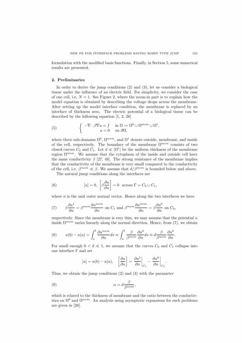
In order to derive the jump conditions (2) and (3), let us consider a biologicaltissue under the influence of an electric field. For simplicity, we consider the caseof one cell, i.e, N = 1. See Figure 2, where the zoom-in part is to explain how themodel equation is obtained by describing the voltage drops across the membrane.After setting up the model interface condition, the membrane is replaced by aninterface of thickness zero. The electric potential of a biological tissue can bedescribed by the following equation [1, 2, 28]

−∇ · β∇u = f in Ω := Ω0 ∪ Ωmem ∪ Ω1,

u = 0 on ∂Ω,(5)

where three sub-domains Ω0, Ωmem, and Ω1 denote outside, membrane, and insideof the cell, respectively. The boundary of the membrane Ωmem consists of twoclosed curves C0 and C1. Let d ≪ |Ω1| be the uniform thickness of the membraneregion Ωmem. We assume that the cytoplasm of the inside and outside cell havethe same conductivity β [27, 48]. The strong resistance of the membrane impliesthat the conductivity of the membrane is very small compared to the conductivityof the cell, i.e. βmem ≪ β. We assume that d/βmem is bounded below and above.

The natural jump conditions along the interfaces are

[u] = 0,

[β∂u

∂n

]= 0 across Γ = C0 ∪C1,(6)

where n is the unit outer normal vector. Hence along the two interfaces we have

β∂u1

∂n= βmem ∂umem

∂non C1 and βmem ∂umem

∂n= β

∂u0

∂non C0,(7)

respectively. Since the membrane is very thin, we may assume that the potential uinside Ωmem varies linearly along the normal direction. Hence, from (7), we obtain

u(b)− u(a) =

∫ b

a

∂umem

∂nds ≈

∫ b

a

β

βmem

∂u0

∂nds ≈ d

β

βmem

∂u0

∂n.(8)

For small enough 0 < d ≪ 1, we assume that the curves C0 and C1 collapse intoone interface Γ and set

[u] = u(b)− u(a),

[∂u

∂n

]=

∂u1

∂n

∣∣∣∣C1

−∂u0

∂n

∣∣∣∣C0

.

Thus, we obtain the jump conditions (2) and (3) with the parameter

(9) α = dβ

βmem,

which is related to the thickness of membrane and the ratio between the conductiv-ities on Ω0 and Ωmem. An analysis using asymptotic expansions for such problemsare given in [28].


Ω1

Ω0

C1 C0

Γ

da b

Ω1

Ωmem

Ω0

Figure 2. A sketch of the domain Ω and local zoom-in near membrane.

2.1. Variational form. In this subsection, we derive a variational formulation forthe problem (1) - (4). For this purpose, we introduce some notations of functionspaces. Let O be any domain and let Hm(O), m = 0, 1, 2 (H0(O) = L2(O)) be

a usual Sobolev space with norm ‖u‖m,O =(∑m

j=0

∫O|∂ju|2dx

)1/2

and we define

the following spaces

Hm(O) := Hm(Ω0 ∩O) ∩Hm(Ω1 ∩O),(10)

HmΓ (O) :=

u : u ∈ Hm(O), [u] = α

∂u0

∂n,

[∂u

∂n

]= 0 on Γ ∩O

,(11)

HmΓ,0(O) :=

u : u ∈ Hm

Γ (O), u|∂O = 0

(12)

equipped with the (semi) norms:

|u|m,O = |u|Hm(O) :=

1∑

i=0

|u|Hm(Ωi∩O), ‖u‖m,O = ‖u‖Hm(O) :=

1∑

i=0

‖u‖Hm(Ωi∩O).

Clearly, HmΓ (Ω) and Hm

Γ,0(Ω) are complete subspaces of Hm(Ω). We also use H10 (Ω)

to denote the space of all functions v ∈ H1(Ω) vanishing on ∂Ω. When the domain is

Ω, we write Hm for Hm(Ω) and denote its norm by ‖u‖Hm . We derive a variational

form of the problem (1)–(4). Multiply (1) by any v ∈ H10 (Ω) and use integration

by parts on each domain to get∫

Ωi

β∇u · ∇v dx =

∫

Ωi

fv dx+

∫

∂Ωi

β∂u

∂niv ds, i = 0, 1,

where ni is the unit outer normal to Ωi. Consider the line integral∫∂Ωi β

∂u∂ni v ds, i =

0, 1. Since we have

1∑

i=0

∫

∂Ωi

β∂u

∂niv ds =

∫

∂Ω0

β∂u

∂n0v ds−

∫

∂Ω1

β∂u

∂n1v ds(13)

= −

∫

Γ

β∂u

∂n[v] ds(14)

= −

∫

Γ

β

α[u][v] ds,(15)


the solution u ∈ H2Γ,0(Ω) of the problem (1) satisfies

a(u, v) :=

1∑

i=0

∫

Ωi

β∇u · ∇v dx+

∫

Γ

β

α[u][v] ds = (f, v), v ∈ H1

0 (Ω).(16)

Conversely, assume u ∈ H2Γ,0 satisfy (16). Integrating by parts, we see the left hand

side of (16) becomes

−

1∑

i=0

∫

Ωi

∇ · (β∇u)vdx +

1∑

i=0

∫

∂Ωi

β∂u

∂niv ds+

∫

Γ

β

α[u][v] ds.(17)

Let v vanish on Γ. Then we have the following equation.

−

1∑

i=0

∫

Ωi

∇ · (β∇u)vdx =

∫

Ω

fv dx, ∀v ∈ H10 (Ω) ∩ v|Γ = 0.

Hence it holds that−∇ · (β∇u) = f in Ω0 ∪ Ω1.

From (16), (17), we have

0 = −

∫

∂Ω0

β∂u

∂n0v ds+

∫

∂Ω1

β∂u

∂n1v ds+

∫

Γ

β

α[u][v] ds,(18)

for all v ∈ H10 (Ω). Choosing v with [v] = 0 on Γ, we see

[∂u

∂n

]= 0 on Γ

and hence, from (18), we obtain the condition (2) by setting v|Ω1 = 0.

3. A new finite element based on P1-Crouzeix-Raviart element

In this section, we propose a finite element for solving the variational form (16).

For this purpose, we need to construct an approximate subspace of H1Γ,0(Ω). At

first glance, a natural approach is to triangularize the domain aligning the gridswith the interface and then discretize the space by piecewise linear functions in-corporating the jump conditions along the interface. However, basis functions haveto be designed to satisfy the jump conditions (2) and (3) along the edge (which isaligned with the interface) of an element. Such process may be a nontrivial matterunless a discontinuous Galerkin method is used. Instead, we propose a new ap-proach with a non-fitted grid, similar to the IFEM, which allows the interface cutthrough the element. In this way, the basis functions are completely determined bythe degrees of freedom and the jump conditions on each element.

Although our method can be applied to any reasonable domains, we take arectangle domain for simplicity. We assume a quasi-uniform triangulation Th ofΩ by triangles of maximum size h is given [16]. In general, the mesh does notalign the smooth interface. We call an element T ∈ Th an interface element if theinterface Γ passes through the interior of T , otherwise we call T a non-interfaceelement.

For a non-interface element T ∈ Th, we simply use the standard P1-Crouzeix-Raviart nonconforming functions [17] on T having the averages along each edge asdegrees of freedom, and use Nh(T ) to denote the linear spaces spanned by the threebasis functions on T : Let ei, i = 1, 2, 3 be the edges of T . Then

Nh(T ) = span

φi : φi is linear on T and φi

∣∣ej

:=1

|ej|

∫

ej

φids = δij , i, j = 1, 2, 3

.


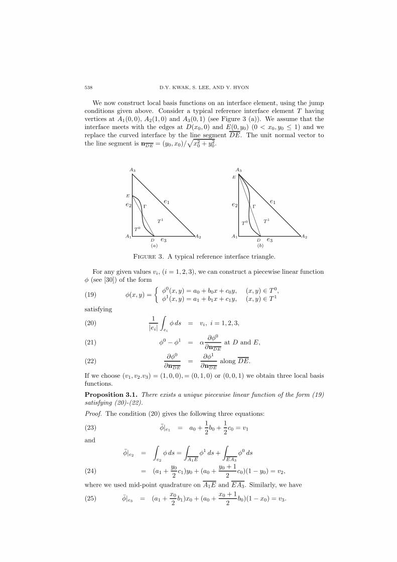
We now construct local basis functions on an interface element, using the jumpconditions given above. Consider a typical reference interface element T havingvertices at A1(0, 0), A2(1, 0) and A3(0, 1) (see Figure 3 (a)). We assume that theinterface meets with the edges at D(x0, 0) and E(0, y0) (0 < x0, y0 ≤ 1) and wereplace the curved interface by the line segment DE. The unit normal vector tothe line segment is n

DE= (y0, x0)/

√x20 + y20 .

A3

A1 A2e3

e1e2

E

D

T 0

T 1

Γ

(a)

A3

A1 A2e3

e1e2

E

D

T 0 T 1

Γ

(b)

Figure 3. A typical reference interface triangle.

For any given values vi, (i = 1, 2, 3), we can construct a piecewise linear functionφ (see [30]) of the form

(19) φ(x, y) =

φ0(x, y) = a0 + b0x+ c0y, (x, y) ∈ T 0,φ1(x, y) = a1 + b1x+ c1y, (x, y) ∈ T 1

satisfying

1

|ei|

∫

ei

φds = vi, i = 1, 2, 3,(20)

φ0 − φ1 = α∂φ0

∂nDE

at D and E,(21)

∂φ0

∂nDE

=∂φ1

∂nDE

along DE.(22)

If we choose (v1, v2.v3) = (1, 0, 0),= (0, 1, 0) or (0, 0, 1) we obtain three local basisfunctions.

Proposition 3.1. There exists a unique piecewise linear function of the form (19)satisfying (20)-(22).

Proof. The condition (20) gives the following three equations:

φ|e1 = a0 +1

2b0 +

1

2c0 = v1(23)

and

φ|e2 =

∫

e2

φds =

∫

A1E

φ1 ds+

∫

EA3

φ0 ds

= (a1 +y02c1)y0 + (a0 +

y0 + 1

2c0)(1 − y0) = v2,(24)

where we used mid-point quadrature on A1E and EA3. Similarly, we have

φ|e3 = (a1 +x0

2b1)x0 + (a0 +

x0 + 1

2b0)(1− x0) = v3.(25)


From the jump condition (21), we have

a0 + b0x0 = a1 + b1x0 + α(b0n1 + c0n2),(26)

a0 + c0y0 = a1 + c1y0 + α(b0n1 + c0n2),(27)

where n1 and n2 are the components of nDE

. The last condition (22) is

(b0n1 + c0n2) = (b1n1 + c1n2).(28)

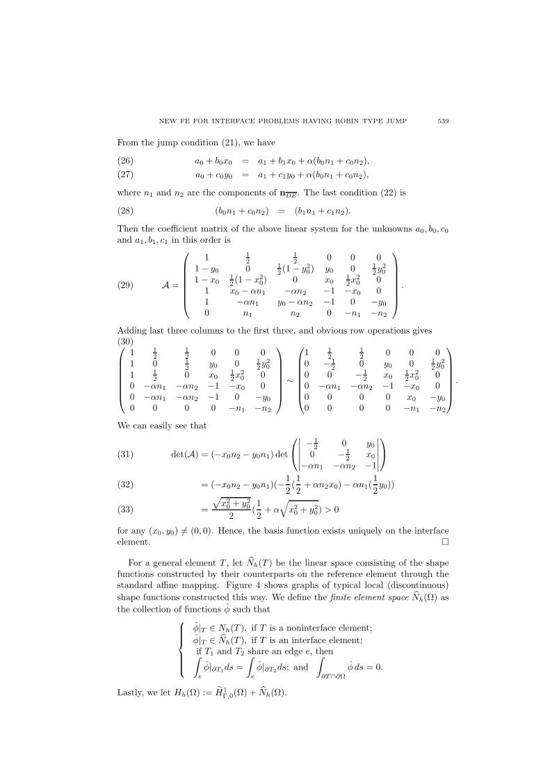
Then the coefficient matrix of the above linear system for the unknowns a0, b0, c0and a1, b1, c1 in this order is

(29) A =

1 12

12 0 0 0

1− y0 0 12 (1− y20) y0 0 1

2y20

1− x012 (1 − x2

0) 0 x012x

20 0

1 x0 − αn1 −αn2 −1 −x0 01 −αn1 y0 − αn2 −1 0 −y00 n1 n2 0 −n1 −n2

.

Adding last three columns to the first three, and obvious row operations gives(30)

1 12

12 0 0 0

1 0 12 y0 0 1

2y20

1 12 0 x0

12x

20 0

0 −αn1 −αn2 −1 −x0 00 −αn1 −αn2 −1 0 −y00 0 0 0 −n1 −n2

∼

1 12

12 0 0 0

0 − 12 0 y0 0 1

2y20

0 0 − 12 x0

12x

20 0

0 −αn1 −αn2 −1 −x0 00 0 0 0 x0 −y00 0 0 0 −n1 −n2

.

We can easily see that

det(A) = (−x0n2 − y0n1) det

∣∣∣∣∣∣

− 12 0 y00 − 1

2 x0

−αn1 −αn2 −1

∣∣∣∣∣∣

(31)

= (−x0n2 − y0n1)(−1

2(1

2+ αn2x0)− αn1(

1

2y0))(32)

=

√x20 + y202

(1

2+ α

√x20 + y20) > 0(33)

for any (x0, y0) 6= (0, 0). Hence, the basis function exists uniquely on the interfaceelement.

For a general element T , let Nh(T ) be the linear space consisting of the shapefunctions constructed by their counterparts on the reference element through thestandard affine mapping. Figure 4 shows graphs of typical local (discontinuous)

shape functions constructed this way. We define the finite element space Nh(Ω) as

the collection of functions φ such that

φ|T ∈ Nh(T ), if T is a noninterface element;

φ|T ∈ Nh(T ), if T is an interface element;if T1 and T2 share an edge e, then∫

e

φ|∂T1ds =

∫

e

φ|∂T2ds; and

∫

∂T∩∂Ω

φ ds = 0.

Lastly, we let Hh(Ω) := H1Γ,0(Ω) + Nh(Ω).


1

Y0

-110.5

0

X

-0.5-1

0.2

0.4

-0.6

-0.4

-0.2

0

-0.5

-0.4

-0.3

-0.2

-0.1

0

0.1

0.2

0.3

10.5

Y

0-0.5

-11

0.5

0

-0.5

X

-1

0

1

2

3

4

-1

-0.5

0

0.5

1

1.5

2

2.5

3

Figure 4. Some shape of functions in Nh(Ω) - left figure shows a

function φ on two interface elements and the right shows a function

φ on six interface elements.

Next, we define the interpolation operator. For any u ∈ H1Γ(T ), we let Ihu be

the the finite element function in Nh(T ) satisfying∫

ei

Ihuds =

∫

ei

u ds; i = 1, 2, 3,

where ei, i = 1, 2, 3 are the edges of T . We call Ihu the local interpolant of u in

Nh(T ) and we naturally extend it to H1Γ(Ω) by (Ihu)|T = Ih(u|T ) for each T .

4. Numerical scheme

In this section, we propose a numerical scheme using the finite element space inSection 3. First, we consider a natural discrete variational formulation of (16): find

the discrete solution uh ∈ Nh(Ω) such that

(34) ah(uh, vh) = (f, vh), ∀vh ∈ Nh(Ω),

where

(35) ah(uh, vh) :=∑

T∈Th

1∑

i=0

∫

T∩Ωi

β∇uh · ∇vh dx +

∫

Γ

β

α[uh][vh] ds,

for uh, vh ∈ Hh(Ω). Since we use the modified CR element, the error in the consis-tency term of (34) is not optimal. From the numerical results in Section 5, we cansee that this scheme does not provide optimal convergence.

To remedy the inconsistency occurred along the boundary of interface elements,we insert consistency and stability terms to the discrete variational formulation.Such ideas are used in many numerical methods, for example, discontinuous Galerkinmethods [6, 5, 11] and IFEMs [32, 43]. For this purpose, we proceed as follows. Thecollection of all interior edges of triangulation Th is denoted by Eh. To determinethe signed jump, we associate a normal ne for each edge e once and for all. Lete ∈ Eh be an interior edge shared by elements T1 and T2. We define the jump [φ]and average φ of function φ ∈ Hh(T1 ∪ T2) on the edge e by

[φ] = φ1 − φ2, φ =1

2(φ1 + φ2),


where φi = φ|Ti, i = 1, 2. Multiplying v ∈ Nh(Ω) to equation (1) and applying

Green’s theorem, we have

∑

T∈Th

1∑

i=0

∫

T∩Ωi

β∇u · ∇v dx−

∫

∂Ωi∩T

β∂u

∂niv ds

−∑

e∈Eh

∫

e

β∂u

∂n

[v] ds =

∑

T∈Th

∫

T

fv dx.(36)

By (13) - (15) and the fact that [u] = 0 for every edge e ∈ Eh, the equation (36) isequivalent to the following equation,

∑

T∈Th

1∑

i=0

∫

T∩Ωi

β∇u · ∇v dx+

∫

Γ∩T

β

α[u][v] ds(37)

−∑

e∈Eh

∫

e

β∂u

∂n

[v] +

β∂v

∂n

[u] ds+

∑

e∈Eh

∫

e

σ

h[u][v] ds =

∑

T∈Th

∫

T

fv dx,(38)

where σ > 0 is some parameter. Now we define the following bilinear form : for

any uh, vh ∈ Nh(Ω),

(39) ah(uh, vh) := ah(uh, vh) + J1(uh, vh) + J2(uh, vh),

where

J1(uh, vh) =−∑

e∈Eh

∫

e

β∂uh

∂n

[vh] +

β∂vh∂n

[uh] ds,(40)

J2(uh, vh) =∑

e∈Eh

∫

e

σ

h[uh][vh] ds.(41)

We are now ready to define our finite element method: find uh ∈ Nh(Ω) such that

ah(uh, φh) = (f, φh), ∀φh ∈ Nh(Ω).(42)

Note that this is a consistent scheme in the sense that for the exact solution u, wehave

ah(u, φh) = (f, φh), ∀φh ∈ Nh(Ω).(43)

4.1. Error estimate. Instead of proving a complete error estimate, we only sketchthe framework using the Lax - Milgram theorem, since most of the techniques arewell known, but the interpolation error estimate seems different from the standardcase. First introduce the mesh dependent norm ||| · ||| on the space Hh(Ω),

|||v|||2 :=∑

T∈Th

∥∥∥√β∇v

∥∥∥2

0,T+

∑

e∈Eh

h−1∥∥∥[√βv]

∥∥∥2

0,e.

Clearly, ah(·, ·) is bounded on Nh(Ω) with respect to ||| · |||:

|ah(u, v)| ≤ Cb|||u||||||v|||, ∀u, v ∈ Nh(Ω).(44)

Next, we can prove the coerciveness of the form ah(·, ·) in a similar fashion to[32], [43].

Lemma 4.1. There exists a positive constant Cc independent of vh such that for

all vh ∈ Nh(Ω) the following holds:

ah(vh, vh) ≥ Cc|||vh|||2.(45)

Then the error estimate reduces to the estimate of interpolation error:


Table 1. Numerical results for the cases of elliptical interface withthe consistent scheme in Example 5.1.

1/h ‖u− uh‖0,Ω Order ‖u− uh‖1,h Order8 3.359148E-2 8.778087E-116 7.480368E-3 2.167 4.307915E-1 1.02732 1.820215E-3 2.039 2.142997E-1 1.00764 4.666885E-4 1.964 1.071044E-1 1.001128 1.161599E-4 2.006 5.343991E-2 1.003256 2.888874E-5 2.008 2.669799E-2 1.001512 7.207460E-6 2.003 1.334396E-2 1.001

Theorem 4.1. Let u (resp. uh) be the solution of (16) (resp. (43). Then thereexists a positive constant C independent of u and h such that

|||u− uh||| ≤ C|||u − Ihu|||.

Proof. By Lemma 4.1, (43), (44) and (45) we get the result.

Remark 4.1. The difficulty of estimating the interpolation error lies in the inap-plicability of the Bramble - Hilbert type Lemma. It is due to the fact that functionsare discontinuous, unlike as earlier case [30]. Since the numerical experiments inSection 5 suggest optimal order of convergence, we leave this topic as a future work.

5. Numerical experiments

We solve the model problem (1)-(3) on the domain Ω = [−1, 1]× [−1, 1] whichis partitioned into uniform right triangles having the base size h = 2−k. For all thenumerical tests, we take β = 1 except Example 5.4 where discontinuous coefficientsβ− = 1, and β+ = 5 are used. We consider various interfaces described by the zerolevel set of some analytic functions. The discrete system is solved by conjugategradient method preconditioned by diagonals. The CPU time (the worst case) isreported for Example 5.5.

Example 5.1. We consider an elliptical interface

Γ =

(x, y) :

x2

a2+

y2

b2= r20

,

where a = 0.7, b = 0.3, and r0 = 1. In this example, we set

α = α0r0/

√x2

a4+

y2

b4,

where α0 = 50.The exact solution is

(46) u =

u− =1

2

(x2

a2+

y2

b2

)− α0r0, for x2

a2 + y2

b2 < r20 ,

u+ =1

2

(x2

a2+

y2

b2

), for x2

a2 + y2

b2 > r20 .

The numerical results by the consistent method are presented in Table 1 and thenumerical solution is plotted in Figure 5. We observe optimal L2- and H1-errors.

For comparison, we also test the inconsistent scheme (34). Table 2 shows thenumerical results of the inconsistent scheme. Although the convergence rate in H1-error maintains the optimal convergence, we see the deterioration of convergence


Figure 5. Plots of numerical solution in Example 1 computed bythe consistent scheme.

rate in L2-error when the mesh becomes finer. Figure 6 shows the plot of thesolution. We observe that the error of the inconsistent method is much larger thanthat of the consistent method. We see that the consistency terms (41) in the bilinearform play an important role in obtaining stable solutions.

Table 2. Numerical results for the cases of elliptical interface withthe inconsistent scheme in Example 5.1


Figure 6. Plots of numerical solution in Example 1 by inconsis-tent scheme.


Example 5.2. In this example, there are four circular interfaces:

Γ1 = (x, y) : (x− 0.5)2 + (y − 0.5)2 − r21 = 0,

Γ2 = (x, y) : (x+ 0.5)2 + (y − 0.5)2 − r22 = 0,

Γ3 = (x, y) : (x+ 0.5)2 + (y + 0.5)2 − r23 = 0,

Γ4 = (x, y) : (x− 0.5)2 + (y + 0.5)2 − r24 = 0,

where (r1, r2, r3, r4) = (0.2, 0.4, 0.2, 0.3). We denote the level-set of Li(x, y) to beinterface Γi. The parameter α is chosen as

(47) α =

α1 =10

L2(x, y)L3(x, y)L4(x, y)on Γ1,

α2 =10


α3 =10


α4 =10

L1(x, y)L2(x, y)L3(x, y)on Γ4.

The exact solution u is

(48) u =

u−1 = L(x, y)− 20r1 if L1(x, y) < 0,

u−2 = L(x, y)− 20r2 if L2(x, y) < 0,

u−3 = L(x, y)− 20r3 if L3(x, y) < 0,

u−4 = L(x, y)− 20r4 if L4(x, y) < 0,

u+ = L(x, y) otherwise,

where L(x, y) = L1(x, y)L2(x, y)L3(x, y)L4(x, y). We observe optimal L2- and H1-errors from Table 3. Figure 7 shows the plot of the numerical solution.

Table 3. Multiple circular interfaces in Example 5.2.


Example 5.3. Here, we carry out a numerical experiment for some problem arisingfrom spectroscopic imaging [1]. We consider the case of nine circular cells in themedium and assume that the properties of each cell are identical. Let the ratiobetween the membrane thickness and the size of the cell be d = 0.7 × 10−3. Theconductivity of the medium and the cell is β = 0.5Sm−1 and the conductivity of themembrane is βmem = 10−8Sm−1. Then by definition of the parameter α in (9), wehave α = 35000. We set the boundary value given by the function sin(xy). Note thatthere is no known analytical solution for this example. The numerical solution isdepicted in Figure 8. We observe that our numerical scheme can capture the jumpof the solution clearly for the problem with realistic parameters.


Figure 7. Numerical solution in Example 5.2.

Y

1

0.5

0

-0.5

-11

0.5

X

0-0.5

-1

0

6000

4000

-2000

-4000

2000

-2000

-1000

0

1000

2000

3000

4000

5000

Figure 8. Numerical solution in Example 5.3.

Example 5.4 (Discontinuous coefficients). We run Example 1 with β− = 1 andβ−+ = 5. We again see optimal result. See Table 3 and left of Figure 9.

Table 4. Distinct β case, β− = 1, β+ = 5.


Example 5.5 (Non convex interface). Finally, we consider a non convex interface(with variable coefficients):

Γ =

(x, y) :

x4

2−

x2

4+ y2 = r20

.


Table 5. Peanut-shaped(Non convex) interface in Example 5.5.


Figure 9. Figures for Examples 5.4 and 5.5.

The exact solution u and α are given by, with r0 = 0.037,

α =0.2

((x3 −

x

4

)2

+ y2)−1/2

,(49)

u =

u− =1

2

(x4

2−

x2

4+ y2

)− 1, when x4

2 − x2

4 + y2 < r20 ,

u+ =1

2

(x4

2−

x2

4+ y2

), when x4

2 − x2

4 + y2 > r20 .(50)

Table 5 and the right of Figure 9 presents the corresponding numerical solution.As a reference, we report the CPU time for the case of 512 × 512 grids was about


26 min. on a window based PC with Intel processor i5-4670, 3.4 Giga Hz. For allother problems, the CPU time was similar.

6. Conclusion and discussion

In this work, we proposed a new numerical method to solve interface problemswhere the jump of primary variable is related to the normal flux. We use CR typeimmersed finite element [30] to construct a new finite element which satisfies theinterface conditions (2) and (3). Our numerical scheme contains consistency andstability terms to compensate the inconsistency along the boundary of the interfaceelements. We observe that our scheme yields optimal convergence of the solutionfor a variety of numerical results. The (interpolation) error analysis of this schemeis left for a future work.

Acknowledgments

The first author is supported by NRF, No. 2014R1A2A1A11053889 and thethird author is supported by NIMS, No. A21100000.

References

[1] H. Ammari, J. Garnier, L. Giovangigli, W. Jing, and J. K. Seo, Spectroscopic imaging of adilute cell suspension, J. Math. Pures Appl. 105 (2016) pp. 603–661.

[2] H. Ammari, J. Garnier, H. Kang, M. Lim, and S. Yu, Generalized Polarization Tensors forShape Description, Numer. Math. 126 (2014) pp. 199–224.

[3] Ph. Angot, Finite volume methods for non smooth solution of diffusion models; applicationto imperfect contact problems in: O.P. Iliev, M.S. Kaschiev, S.D. Margenov, Bl.H. Sendov,P.S. Vassilevski (Eds.), Recent Advances in Numerical Methods and Applications. Proc. 4thInt. Conf. NMA98, Sofia (Bulgarie), World Sci. Pub., (1999) pp. 621–629.

[4] Ph. Angot, A unified fictitious domain model for general embedded boundary conditions,C. R. Acad. Sci. Paris, Serie I Math. 341 (2005), no. 11, pp. 683–688.

[5] D. N. Arnold, An interior penalty finite element method with discontinuous elements, SIAMJ. Numer. Anal. 19 (1982) pp. 742–760.

[6] D. N. Arnold, F. Brezzi, B. Cockburn, and L. D. Marini, Unified analysis of discontinuousGalerkin methods for elliptic problems, SIAM J. Numer. Anal. 39 (2001) pp. 1749–1779.

[7] M. Bean and Son-Young Yi, An immersed interface method for a 1D poroelasticity problemwith discontinuous coefficients, J. Comp. App. Math., V 272, (2014), pp. 81–96.

[8] R. Becker, E. Burman, and P. Hansbo, A Nitsche extended finite element method forincompressible elasticity with discontinuous modulus of elasticity, Comp. Methods Appl.Mech. Engrg. 198 (2009) pp. 3352–3360.

[9] A. Bermudez, R. Duran, and R. Rodriguez, Finite element solution of incompressible FluidStructure vibration problems, Internat. J. Numer. Methods Engrg. 40 (1997) pp. 1435–1448.

[10] P. A. Berthelsen, A decomposed immersed interface method for variable coefficient ellipticequations with non-smooth and discontinuous solutions, J. Comp. Phys. 197 (2004) pp.364–386.

[11] F. Brezzi, G. Manzini, D. Marini, P. Pietra, and A. Russo, Discontinuous Galerkin approx-imations for elliptic problems, Numer. Meth. P.D.E. 16 (2000) pp. 365–378.

[12] E. Burman, Ghost penalty, C. R. Math Acad Sci Paris 348 (2010), pp. 1217–1220.[13] K. S. Chang and Do Y. Kwak, Discontinuous Bubble scheme for elliptic problems with

jumps in the solution, Comp. Meth. Appl. Mech. Engrg. 200 (2011) pp. 494–508.[14] S. H. Chou, D. Y. Kwak, and K. T. Wee, Optimal convergence analysis of an immersed

interface finite element method, Adv. Comp. Math, 33 (2010) pp. 149–168.[15] Z. Chen and J. Zou, Finite element methods and their convergence for elliptic and parabolic

interface problems, Numer. Math. 79 (1998) pp. 175–202.[16] P. G. Ciarlet, The finite element method for elliptic problems, North Holland 1978.[17] M. Crouzeix and P. A. Raviart, Conforming and nonconforming finite element methods for

solving the stationary Stokes equations, RAIRO Anal. Numer. 7 (1973) pp. 33–75.[18] Y. Gong, B. Li, and Z. Li, Immersed-interface finite-element methods for elliptic interface

problems with nonhomogeneous jump conditions, SIAM J. Numer. Anal. 46 (2008) pp.472–495.


[19] S. Groβ, V. Reichelt, and A. Reusken, A finite element based level set method for two-phaseincompressible flows, Comp. Visual Sci. 9 (2006) pp. 239–257.

[20] G. Guyomarc’h, C. O. Lee, and K. Jeon, A discontinuous Galerkin method for ellipticinterface problems with application to electroporation, Commun. Numer. Meth. Engng 25(2009) pp. 991–1008.

[21] A. Hansbo and P. Hansbo, An unfitted finite element method, based on Nitsche’s method,for elliptic interface problems, Comp. Methods Appl. Mech. Engrg. 191 (2002) pp. 5537–5552.

[22] A. Hansbo and P. Hansbo, A finite element method for the simulation of strong and weakdiscontinuities in solid mechanics, Comp. Methods Appl. Mech. Engrg. 193 (2004) pp. 3523–3540.

[23] X. He, T. Lin, and Y. Lin, Immersed finite element methods for elliptic interface problemswith non-homogeneous jump conditions, Int. J. Numer. Anal. Model. 8 (2011) pp. 284–301.

[24] X. He, T. Lin, Y. Lin, and X. Zhang, Immersed finite element methods for parabolicequations with moving interface, Numer. Methods P.D.E, 29 (2013) pp. 619–646.

[25] Ji, H. F., Chen, J. R., & Li, Z. L., A symmetric and consistent immersed finite elementmethod for interface problems, J. of Sci. Comp., 61 (2014) pp. 533-557.

[26] H. Ji, J.u Chen, F. Wang, Unfitted finite element methods for the heat conduction incomposite media with contact resistance, Numer. Meth. P.D.Es, 33(1) (2017) pp. 354-380.

[27] J. Keener and J. Sneyd, Mathematical Physiology, Springer New York 2009.[28] A. Khelifia and H. Zribib, Asymptotic expansions for the voltage potentials with two-

dimensional and three-dimensional thin interfaces, Math. Meth. Appl. Sci. 34 (2011) pp.2274–2290.

[29] S. Kim, J. K. Seo, and T. Ha, A Nondestructive Evaluation Method for Concrete Voids:Frequency Differential Electrical Impedance Scanning, SIAM J. Appl. Math. 69 (2009) pp.1759–1771.

[30] D. Y. Kwak, K. T. Wee, and K. S. Chang, An analysis of a broken P1-nonconforming finiteelement method for interface problems, SIAM J. Numer. Aanal. 48 (2012) pp. 2117–2134.

[31] D. Y. Kwak, S. Jin, and D. Kyeong , A stabilized P1-immersed finite element method forthe interface for elasticity problems, ESAIM: M2AN, V. 51 (2017) pp. 187–207.

[32] D. Y. Kwak and J. Lee, A modified P1-immersed finite element method, Int. J. Pure Appl.Math. 104 (2015) pp. 471–494.

[33] I. Lackovic, R. Magjarevic, and D. Miklavcic, Analysis of Tissue Heating During Electro-poration Based Therapy: A 3D FEM Model for a Pair of Needle Electrodes, Medicon 2007IFMBE Proceedings 16, (2007) pp. 631–634.

[34] W. J. Layton, F. Schieweck, and I. Yotov, Coupling fluid flow with porous media flow,SIAM J. Numer. Anal. 40, (2002), 2195-2218.

[35] R. J. LeVeque and Z. Li, The immersed interface method for elliptic equations with discon-

tinuous coefficients and singular sources, SIAM J. Numer. Anal. 31 (1994) pp. 1019–1044.[36] R. J. LeVeque and Z. Li, Immersed interface method for Stokes flow with elastic boundaries

or surface tension, SIAM J. Sci. Comp. 18 (1997) pp. 709–735.[37] Z. Li, The immersed interface method using a finite element formulation, Applied Numer.

Math. 27 (1998) pp. 253–267.[38] Z. Li, Immersed interface method for moving interface problems, Numer. Algorithms 14

(1997) pp. 269–293.[39] Z. Li and K. Ito, The immersed interface method: Numerical solutions of PDEs involving

interfaces and irregular domains, Front. Appl. Math. 33, SIAM, Phil. 2006.[40] Z. Li, T. Lin, Y. Lin, and R. C. Rogers, An immersed finite element space and its approxi-

mation capability, Numer. Methods. P.D.E. 20 (2004) pp. 338–367.[41] Z. Li, T. Lin, and X. Wu, New Cartesian grid methods for interface problems using the

finite element formulation, Numer. Math. 96 (2003) pp. 61–98.[42] T. Lin, Y. Lin, and X. Zhang, A method of lines based on immersed finite elements for

parabolic moving interface problems, Adv. Appl. Math. Mech. 5 (2013) pp. 548–568.[43] T. Lin, Y. Lin, and X. Zhang, Partially Penalized Immersed Finite Element Methods For

Elliptic Interface Problems, SIAM J. Numer. Anal. V. 53 (2), 2015, pp.1121–1144.[44] T. Lin, D. Sheen and X. Zhang, A locking-free immersed finite element method for planar

elasticity interface problems, J. of Comp. Phys, 247 (2013) pp. 228–247.[45] D. Kyeong and D. Y. Kwak, An immersed finite element method for the elasticity problems

with displacement jump, Advances in Applied Mathematics and Mechanics, V. 9, No. 2,(2017) pp. 407–428.


[46] I. Ramirere, Ph. Angot, and M. Belliard, A fictitious domain approach with spread interfacefor elliptic problems with general boundary conditions, Comp. Meth. in Appl. Mech. andEngrng. 196 (2007) pp. 766–781.

[47] Beatrice Riviere, Analysis of a Discontinuous Finite Element Method for the Coupled Stokesand Darcy Problems, J. of Sci. Computing, Vols 22 (2005) pp. 479– 500.

[48] T. Suna, S. Tsudab, K.-P. Zaunerb, and H. Morgana, On-chip electrical impedance tomog-raphy for imaging biological cells, Biosensors and Bioelectronics 25 (2010) pp. 1109–1115.

Korea Advanced Institute of Science and Technology, Daejeon, Korea 34141.E-mail : email:[email protected]

Korea Advanced Institute of Science and Technology, Daejeon, Korea 34141.E-mail : email:[email protected]

National Institute for Mathematical Sciences, Daejeon, Korea 34047.E-mail : email:[email protected]

a new finite element for interface problems having … · abstract. we propose a new ﬁnite...

Documents