a new lifetime distribution: transmuted exponential …

Commun.Fac.Sci.Univ.Ank.Ser. A1 Math. Stat.Volume 70, Number 1, Pages 1—14 (2021)DOI: 10.31801/cfsuasmas.528306ISSN 1303—5991 E-ISSN 2618—6470

https://communications.science.ankara.edu.tr

Received by the editors: February 18, 2020; Accepted: October 26, 2020

A NEW LIFETIME DISTRIBUTION: TRANSMUTEDEXPONENTIAL POWER DISTRIBUTION

Bugra SARACOGLU and Caner TANIS

Department of Statistics, Selcuk University,Konya, TURKEY

Abstract. In this paper, we have introduced a new statistical distributioncalled as transmuted Exponential Power (TEP) distribution using the qua-dratic rank transmutation map proposed by Shaw and Buckley [25,26] in orderto generate new distributions. We have also studied some statistical propertiessuch as descriptive statistics (moments, variance, coeffi cient of skewness (CS)and kurtosis (CK)), point estimation (maximum likelihood estimation) andreal data applications to illustrate usefulness of TEP distribution.

1. Introduction

In statistical literature, several lifetime distributions are introduced. Most ofthese distributions are generally obtained by compounding or mixing methodolo-gies. In the other case, distributions are given through including an extra parameterto well-known distribution. By the way, family of distributions obtained using qua-dratic rank transmutation map (QRTM) proposed by Shaw and Buckley [25,26] isdefined with cumulative distribution function (cdf) and probability density function(pdf)

F (x) = (1 + λ)G(x)− λ [G(x)]2 (1)

andf(x) = (1 + λ)g(x)− 2λG(x)g(x), (2)

respectively, where G(x) denotes cdf of baseline distribution and λ ∈ [−1, 1] istransmuting parameter. If λ = 0, cdf of the base distribution is obtained. In lastdecade, there are many studies about transmuted distributions in literature. For

2020 Mathematics Subject Classification. Primary 60E05; Secondary 62F10.Keywords and phrases. Transmuted exponential power distribution, Quadratic rank transmu-

tation map, Maximum likelihood [email protected] author; [email protected]; 0000-0003-0090-1661.

c©2020 Ankara UniversityCommunications Facu lty of Sciences University of Ankara-Series A1 Mathematics and Statistics

1

2 B. SARACOGLU, C. TANIS

example; Aryal and Tsokos [3,4] introduced transmuted Weibull and transmuted ex-treme value distributions. Ashour and Eltehiwy [5,6] proposed transmuted Lomaxand transmuted exponentiated Lomax distributions, Merovci [18—21] introducedtransmuted Rayleigh, transmuted Lindley, transmuted generalized Rayleigh andtransmuted exponentiated Exponential distributions, Mahmoud and Mandouh [17]suggested transmuted Frechet distribution, Hussian [13] has introduced transmutedexponentiated Gamma distribution, Elbatal and Aryal [10] studied transmuted ad-ditive Weibull distribution, Khan et al. [14—16] introduced transmuted Weibulldistribution, transmuted Kumaraswamy distribution and transmuted generalizedGompertz distribution, Shahzad and Asghar [24] proposed transmuted Dagum dis-tribution, Al-Babtain et.al. [2] introduced the Kumaraswamy-transmuted exponen-tiated modified Weibull distribution.Over two decades before, Smith and Bain [23] introduced the Exponential Power

(EP) distribution by compounding exponential and Weibull distribution functions.The cdf and pdf of EP distribution are given

G (x;α, β) = 1− exp[1− exp

((xα

)β)](3)

and

g (x;α, β) =β

α

(xα

)β−1exp

((xα

)β)exp

[1− exp

((xα

)β)], (4)

respectively, where α > 0, β > 0 and x > 0. Many authors have focused on EPdistribution recently. Some of these studies can be listed as follows; Chen [8],Barriga et al. [7], Akdam et al. [1].The main purpose of this study is to suggest a new lifetime distribution as

an alternative EP distribution by using QRTM. In Section 2, TEP distributionand its some statistical properties (moments, variance, CS, CK) are introduced.The maximum likelihood estimators (MLEs) for unknown parameters of introduceddistribution are derived in Section 3. In Section 4, a Monte Carlo simulation studyis performed to evaluate the performances of these estimators in terms of meansquare errors (MSEs) and bias. In Section 5, two real data illustrations are given toshow the applicability of this distribution in real life. In Section 6, the conclusionremarks are given.

2. Transmuted Exponential Power (TEP) Distribution

Let X be a random variable having TEP distribution with α, β and λ parametersdenoted by TEP(α, β, λ). The cdf and pdf of this random variable are

F (x;α, β, λ) = (1 + λ)[1− exp

(1− exp

((xα

)β))]−λ[1− exp

(1− exp

((xα

)β))]2 (5)

A NEW LIFETIME DISTRIBUTION 3

and

f(x;α, β, λ) = βα

(xα

)β−1exp

((xα

)β)exp

[1− exp

((xα

)β)]×[1 + λ− 2λ

(1− exp

(1− exp

((xα

)β)))] , (6)

respectively. Where −1 ≤ λ ≤ 1, α, β > 0 and x > 0. The cdf of EP distributionfor λ = 0 in Eq. (5) is derived. Figure 1 shows the possible shapes of the pdf ofTEP distribution for various parameter values.

Figure 1. Plots of the TEP density function for various values ofα, β and λ

The reliability function (rf ) and hazard function (hf ) of TEP distribution aredefined as

R(t) = 1− (1 + λ)[1− exp

(1− exp

((tα

)β))]+λ[1− exp

(1− exp

((tα

)β))]2 (7)

and

h(t) =βα (

tα )

β−1exp

(( tα )

β)k(t,α,β)

1−(1+λ)[1−k(t,α,β)]+λ[1−k(t,α,β)]2

× [1 + λ− 2λ (1− k(t, α, β))] ,(8)

respectively. Where k(t, α, β) = exp[1− exp

((tα

)β)]. Figure 2 shows that the

possible shapes of (hf ) for TEP distribution at different parameter values.


Figure 2. Plots of the TEP hazard function for various values ofα, β and λ

2.1. Moments of TEP distribution. The rth moment of TEP distribution is

E(Xr) =∫∞0xr ((1 + λ)g(x)− 2λG(x)g(x)) dx

= ((1 + λ)I1 − 2λI2)(9)

where I1 and I2 are

I1 =

∫ ∞0

xrg(x)dx

=

∫ ∞0

xrβ

α

(xα

)β−1exp

((xα

)β)s(x, α, β)dx

=

∞∑n=0

1

n!αr∫ ∞1

(ln(u))n+(r/β) e

1−u

udu (10)

and

I2 =

∫ ∞0

xrG(x)g(x)dx

=

∫ ∞0

xr [1− s(x, α, β)] βα

(xα

)β−1exp

((xα

)β)s(x, α, β)dx

= I1 −∞∑n=0

1

n!αr∫ ∞1

(ln(u))n+(r/β) e

2−2u

udu, (11)


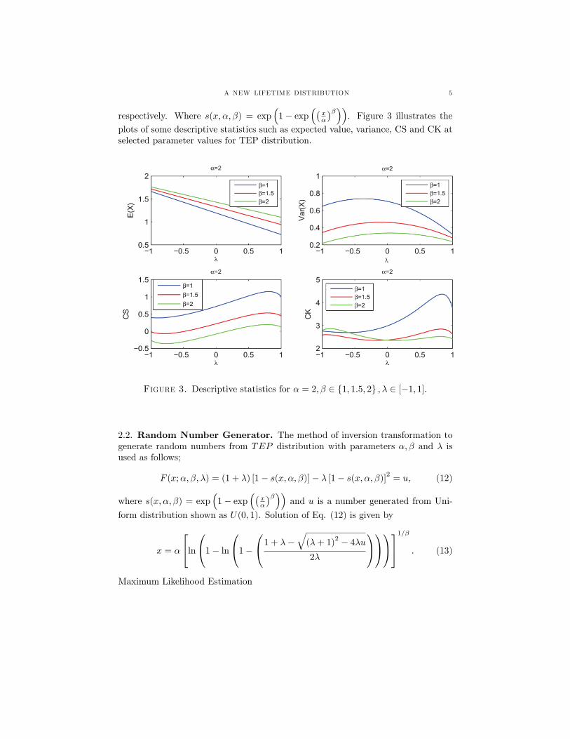
respectively. Where s(x, α, β) = exp(1− exp

((xα

)β)). Figure 3 illustrates the

plots of some descriptive statistics such as expected value, variance, CS and CK atselected parameter values for TEP distribution.

Figure 3. Descriptive statistics for α = 2, β ∈ {1, 1.5, 2} , λ ∈ [−1, 1].

2.2. Random Number Generator. The method of inversion transformation togenerate random numbers from TEP distribution with parameters α, β and λ isused as follows;

F (x;α, β, λ) = (1 + λ) [1− s(x, α, β)]− λ [1− s(x, α, β)]2 = u, (12)

where s(x, α, β) = exp(1− exp

((xα

)β))and u is a number generated from Uni-

form distribution shown as U(0, 1). Solution of Eq. (12) is given by

x = α

ln1− ln

1−1 + λ−

√(λ+ 1)

2 − 4λu2λ

1/β . (13)

Maximum Likelihood Estimation


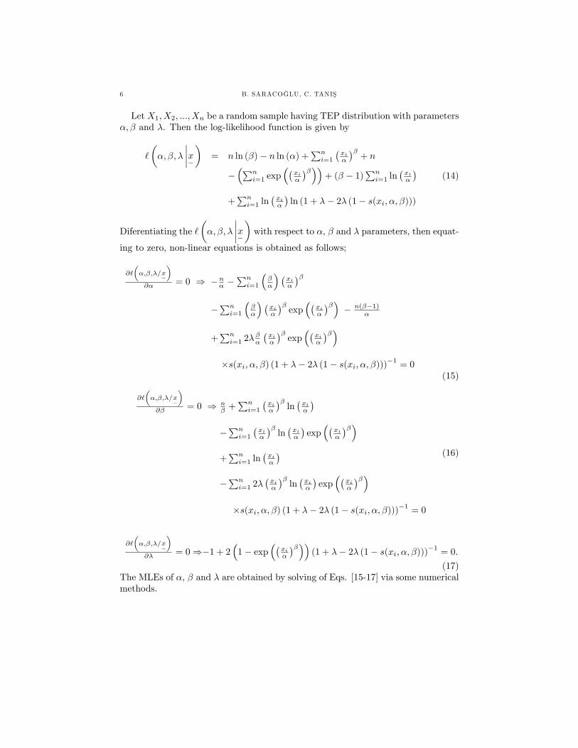
Let X1, X2, ..., Xn be a random sample having TEP distribution with parametersα, β and λ. Then the log-likelihood function is given by

`

(α, β, λ

∣∣∣∣x−)

= n ln (β)− n ln (α) +∑ni=1

(xiα

)β+ n

−(∑n

i=1 exp((

xiα

)β))+ (β − 1)

∑ni=1 ln

(xiα

)+∑ni=1 ln

(xiα

)ln (1 + λ− 2λ (1− s(xi, α, β)))

(14)

Diferentiating the `(α, β, λ

∣∣∣∣x−)with respect to α, β and λ parameters, then equat-

ing to zero, non-linear equations is obtained as follows;

∂`

(α,β,λ/x

−

)∂α = 0 ⇒ −nα −

∑ni=1

(βα

) (xiα

)β−∑ni=1

(βα

) (xiα

)βexp

((xiα

)β) − n(β−1)α

+∑ni=1 2λ

βα

(xiα

)βexp

((xiα

)β)×s(xi, α, β) (1 + λ− 2λ (1− s(xi, α, β)))−1 = 0

(15)

∂`

(α,β,λ/x

−

)∂β = 0 ⇒ n

β +∑ni=1

(xiα

)βln(xiα

)−∑ni=1

(xiα

)βln(xiα

)exp

((xiα

)β)+∑ni=1 ln

(xiα

)−∑ni=1 2λ

(xiα

)βln(xiα

)exp

((xiα

)β)×s(xi, α, β) (1 + λ− 2λ (1− s(xi, α, β)))−1 = 0

(16)

∂`

(α,β,λ/x

−

)∂λ = 0⇒−1 + 2

(1− exp

((xiα

)β))(1 + λ− 2λ (1− s(xi, α, β)))−1 = 0.

(17)The MLEs of α, β and λ are obtained by solving of Eqs. [15-17] via some numericalmethods.


Table 1. The MSEs and biases of α,β and λ.bias MSE

n parameter values α β λ α β λ5 -0.4738 0.7255 -0.8020 0.5023 1.1866 0.736810 -0.3492 0.2620 -0.6064 0.2502 0.1958 0.485520 -0.3460 0.1159 -0.4095 0.1858 0.0498 0.245250 (2,0.8,0.1) -0.3439 0.0578 -0.2558 0.1510 0.0126 0.0796100 -0.3314 0.0433 -0.2167 0.1320 0.0061 0.0532300 -0.2863 0.0275 -0.1834 0.1052 0.0022 0.04285 0.0533 0.5609 0.6402 0.0274 0.7886 0.448510 0.0698 0.3201 0.5680 0.0195 0.2037 0.383020 0.0689 0.2132 0.4810 0.0138 0.0872 0.327750 (0.4,0.6,-0.8) 0.0582 0.1328 0.3541 0.0099 0.0398 0.2559100 0.0424 0.0886 0.2503 0.0071 0.0241 0.1916300 0.0198 0.0382 0.1148 0.0035 0.0101 0.09615 -0.3532 0.7178 -0.3549 0.3446 2.5125 0.217610 -0.2487 0.2176 -0.3094 0.1959 0.5131 0.224820 -0.1759 0.0386 -0.2589 0.1183 0.1932 0.221250 (3,2,0.5) -0.1123 -0.0391 -0.1976 0.0746 0.0882 0.1997100 -0.0832 -0.0620 -0.1645 0.0608 0.0610 0.1821300 -0.0273 -0.0457 -0.0754 0.0403 0.0308 0.11835 -0.0513 0.1908 -0.6024 0.0257 0.1503 0.454910 -0.0563 0.0490 -0.4850 0.0173 0.0248 0.363420 -0.0671 0.0091 -0.4005 0.0137 0.0080 0.302750 (0.3,0.4,0.8) -0.0630 -0.0041 -0.2968 0.0104 0.0031 0.2163100 -0.0516 -0.0052 -0.2235 0.0082 0.0017 0.1495300 -0.0310 -0.0047 -0.1314 0.0058 0.0006 0.0783

3. Simulation Study

In this section, a Monte Carlo simulation study is performed to evaluate theperformances of MLEs according to MSEs and biases. Algorithm steps regardingto simulation study are as follows;Step 1. Random numbers are generated from TEP distribution with parameters

α, β and λ by using Eq. (13).Step 2. MLEs of α, β and λ are calculated by using Eqs. (15)-(17) as based on

10000 replicates.Step 3. The biases and MSEs of these estimators are simulated for different

sample sizes as 5,10, 20, 50, 100 and 300 at selected parameter values ((α, β, λ) =(2, 0.8, 0.1), (0.4, 0.6,−0.8),(3, 2.0.5), and (0.3, 0.4, 0.8)).The results of simulation study are presented in

Table 1.According to Table 1, it is clearly seen that the MSEs and biases of MLEs for

all parameter cases decrease as sample sizes increases. This case indicates thatestimate values approach to true values as sample size n increases.


4. Real Data Analysis

In this section, we aim to compare TEP distribution with other distributionsin terms of goodness of fit measures to demonstrate the applicability of TEP dis-tribution. Two real data sets have been used for these purposes. We have con-sidered some goodness of fit measures such as the Akaike’s Information Criterion(AIC), corrected Akaike’s Information Criterion (AICc), -2×log-likelihood value,Kolmogorov-Smirnov (KS) statistics and its p-value to compare the fits of the dis-tributions for two data sets. These statistics are given as follows;

AIC = −2`+ 2k, (18)

AICc = AIC +

(2k(k + 1)

n− k − 1

), (19)

KS = sup (|F (x)− Fn(x)|) . (20)

where k is number of parameters, n is sample size, ` is the value of log-likelihoodfunction.

4.1. Operation and empirical data. The first real data set consist of 50 obser-vations has been obtained by Dasgupta [9]. This data set relates to holes operationon jobs made of iron sheet is given by in Table 2.

Table 2. Operation and empirical data0.04 0.02 0.06 0.12 0.14 0.08 0.22 0.12 0.08 0.260.24 0.04 0.14 0.16 0.08 0.26 0.32 0.28 0.14 0.160.24 0.22 0.12 0.18 0.24 0.32 0.16 0.14 0.08 0.160.24 0.16 0.32 0.18 0.24 0.22 0.16 0.12 0.24 0.060.02 0.18 0.22 0.14 0.06 0.04 0.14 0.26 0.18 0.16

These data have been fitted to TEP, generalized Gompertz (GG) [11], transmutedgeneralized Gompertz (TGG) [16], transmuted Kumaraswamy (TKw) [14], trans-muted Rayleigh (TR) [18], transmuted exponentiated exponential (TEE) [21] andtransmuted Weibull (TW) [3] distributions. The density functions of the fitted


Table 3. Parameter estimates(standard errors) for operation and empirical dataDistribution MLEs

TEPα = 0.2400 (0.0327) , β = 1.5996 (0.4081) ,

λ = −0.0234 (0.7000)

TGGa = 3.0808 (3.2536) , b = 7.5224 (4.2694) ,

α = 1.3521 (0.5060) , λ = −0.1075 (0.9151)

GG a = 2.5012 (1.6916) , b = 8.3737 (3.0939) ,α = 1.2784 (0.4692)

TKwa = 1.9335 (0.3524) , b = 30.1864 (13.7921) ,

λ = −0.2911 (0.4408)TR σ = 0.1211 (0.0110) , λ = −0.2645 (0.3086)

TWµ = 1.9917 (0.3310) , σ = 0.1708 (0.0236) ,

λ = −0.2722 (0.4308)

TEEθ = 2.6946 (0.8398) , α = 12.4959 (1.6663) ,

λ = −0.5468 (0.3189)

distributions are given by;

TGG : f(x) = αaebxe(−ab (e

(bx)−1))[1− e(− ab (e

((bx)−1)))]α−1

×[1 + λ− 2λ

(1− e(− ab e

((bx)−1)))α]

, x > 0, a, b, α > 0, λ ∈ [−1, 1]

GG : f(x) = αaebxe(−ab (e

(bx)−1))[1− e(− ab (e

((bx)−1)))]α−1

, x > 0, a, b, α > 0

TEE : f(x) = θα (1− e−αx)θ−1 e−αx[1 + λ− 2λ (1− e−αx)θ

], x > 0, a, θ > 0, λ ∈ [−1, 1]

TKw : f (x) = abxa−1 (1− xa)b−1[1− λ+ 2λ (1− xa)b

], x ∈ [0, 1] , a, b > 0, ,λ ∈ [−1, 1]

TR : f (x) = xσ2 e− x2

2σ2

[1− λ+ 2λe−

x2

2σ2

], x > 0, σ > 0,λ ∈ [−1, 1]

TW : f (x) = µσ

(xσ

)µ−1e−(

xσ )

µ [1− λ+ 2λe−( xσ )

µ], x > 0, µ, σ > 0, λ ∈ [−1, 1]

For operation and empirical data set, the MLEs (standard errors) of fitted distri-butions are given in Table 3 and the selection criteria statistics are given in Table4. Furthermore, The plots which shows fits of distributions to this data set can beexamined from Figure 4 and Figure 5.

4.2. Breaking Stress data. The second data set is with regard to breaking stressof carbon fibers of 50 mm length (GPa) obtained by Nichols and Padgett [22]. This


Table 4. Selection criteria statistics for operation and empirical dataDistribution -2log AIC AICc K-S p-value

TEP -114.9401 -108.9401 -108.4184 0.0893 0.8199TGG -114.5400 -106.5400 -105.6520 0.0898 0.8152GG -114.5924 -108.5924 -108.0707 0.0936 0.7736TKw -112.5020 -106.5020 -105.9800 0.1052 0.6375TR -112.1173 -108.1173 -107.8620 0.1070 0.6162TW -112.1179 -106.1179 -105.5962 0.1070 0.6163TEE -106.5607 -100.5607 -100.0389 0.1462 0.2357

Figure 4. Empirical cdf and fitted cdfs for operation and empir-ical data set

data set consist of 66 observations has been used by Yousof et.al. [27]. The breakingstress data are presented in Table 5.

Table 5. Breaking stress data0.39 0.85 1.08 1.25 1.47 1.57 1.61 1.61 1.69 1.80 1.841.87 1.89 2.03 2.03 2.05 2.12 2.35 2.41 2.43 2.48 2.502.53 2.55 2.55 2.56 2.59 2.67 2.73 2.74 2.79 2.81 2.822.85 2.87 2.88 2.93 2.95 2.96 2.97 3.09 3.11 3.11 3.153.15 3.19 3.22 3.22 3.27 3.28 3.31 3.31 3.33 3.39 3.393.56 3.60 3.65 3.68 3.70 3.75 4.20 4.38 4.42 4.70 4.90

This data set has been fitted to TEP, exponential power (EP) [23], exponenti-ated exponential (EE) [12], transmuted exponentiated exponential (TEE) [21] and


Figure 5. Fitted pdfs for operation and empirical data set

transmuted Rayleigh (TR) [18] distributions. The density functions of the fitteddistributions are given by;

EP : f (x) = βα

(xα

)β−1exp

((xα

)β)exp

[1− exp

((xα

)β)], x > 0, α, β > 0

EE : f (x) = θα (1− e−αx)θ−1 e−αx , x > 0, α, θ > 0

TR : f (x) = xσ2 e− x2

2σ2

[1− λ+ 2λe−

x2

2σ2

], x > 0, σ > 0, λ ∈ [−1, 1]

TEE : f (x) = θα (1− e−αx)θ−1

×e−αx[1 + λ− 2λ (1− e−αx)θ

], x > 0, α, θ > 0, λ ∈ [−1, 1]

The MLEs of unknown parameters for these distributions and their standard errorsare shown in Table 6.

For breaking stress data, the comparison statistics of fitted distributions are givenin Table 7. Also, the goodness of fit plots based on the empirical and theoreticalcdfs and pdfs of fitted distributions can be seen from Figure 6 and Figure 7.

Table 7. Selection criteria statistics for breaking stress data


Table 6. Parameter estimates(standard errors) for breaking stress dataDistribution MLEs

TEPα = 4.0683 (0.2181) , β = 2.8374 (0.2716) ,

λ = 0.7487 (0.2503)

EP α = 3.6807 (0.1182) , β = 2.3799 (0.2304)

EE θ = 9.1992 (2.1491) , α = 1.0076 (0.1002)

TEEθ = 7.4605 (2.1903) , α = 1.1195 (0.1089) ,

λ = −0.7773 (0.1812)TR σ = 1.6957 (0.0825) , λ = −0.9587 (0.0930)

Distribution -2log AIC AICc K-S p-valueTEP 172.4577 178.4577 178.8448 0.0913 0.6408EP 174.7949 178.7949 178.9854 0.1126 0.3724EE 190.7447 194.7447 194.9352 0.1550 0.0840TEE 185.0412 191.0412 191.4283 0.1344 0.1844TR 177.7488 183.7488 184.1359 0.1410 0.1447

Figure 6. Empirical cdf and fitted cdfs for breaking stress data

5. Conclusion

In this study, we have proposed a new lifetime distribution which can be usedas an alternative of EP distribution called as TEP. This new distribution havingincreasing, decrasing and bathtube hazard rate function has more flexibility than


Figure 7. Fitted pdfs for breaking stress data

EP distribution. From two real data applications, it can have been concludedthat TEP distribution has the best fitting among other fitted distributions. Thesereal data applications show that TEP distribution is usefullness for modelling realdata such as carbon fibres, operation and empirical data sets. These areas ofapplication can be extended by using various real data sets which show fitting toTEP distribution.

References

[1] Akdam, N., Kinaci, I., Saracoglu, B., Statistical inference of stress-strength reliability for theexponential power (EP) distribution based on progressive type-II censored samples, HacettepeJournal of Mathematics and Statistics, 46 (2017), 239-253.

[2] Al-Babtain, A., Fattah, A. A., Ahmed, A. H. N., Merovci, F., The Kumaraswamy-transmutedexponentiated modified Weibull distribution, Communications in Statistics-Simulation andComputation, 46 (2017), 3812-3832.

[3] Aryal, G. R., Tsokos, C. P., Transmuted Weibull distribution: A generalization of the Weibullprobability distribution, European Journal of Pure and Applied Mathematics 4 (2011), 89-102.

[4] Aryal, G. R., Tsokos, C. P., On the transmuted extreme value distribution with application,Nonlinear Analysis: Theory, Methods & Applications, 71 (2009), 1401-1407.

[5] Ashour, S. K., Eltehiwy, M. A., Transmuted exponentiated Lomax distribution, Aust J BasicAppl Sci, 7 (2013), 658-667.

[6] Ashour, S. K., Eltehiwy, M. A., Transmuted lomax distribution, American Journal of AppliedMathematics and Statistics, 1 (2013), 121-127.

[7] Barriga, G. D., Louzada-Neto, F., Cancho, V. G. The complementary exponential powerlifetime model, Computational statistics and data analysis, 55(3) (2011), 1250-1259.

[8] Chen Z. Statistical inference about the shape parameter of the exponential power distribu-tion.Statistical Papers, 40(1) (1999), 459-468.


[9] Dasgupta, R., On the distribution of burr with applications, Sankhya B, 73 (2011), 1-19.[10] Elbatal, I., Aryal, G., On the Transmuted Additive Weibull Distribution, Austrian Journal

of Statistics, 42 (2016), 117-132.[11] El-Gohary, A., Alshamrani, A., Al-Otaibi, A. N., The generalized Gompertz distribution,

Applied Mathematical Modelling, 37 (1-2) (2013), 13-24.[12] Gupta, R. D., Kundu, D., Exponentiated exponential family: an alternative to gamma and

Weibull distributions, Biometrical journal, 43 (2001), 117-130.[13] Hussian, M. A., Transmuted exponentiated gamma distribution: A generalization of the ex-

ponentiated gamma probability distribution, Applied Mathematical Sciences, 8 (2014), 1297-1310.

[14] Khan, M S., King, R. and Hudson, I L., Transmuted Kumaraswamy Distribution. Statisticsin Transition new series, 17 (2016), 183-210.

[15] Khan, M. S., King, R. and & Hudson, I L., Transmuted Weibull distribution: Properties andestimation, Communications in Statistics-Theory and Methods, 46 (2017), 5394-5418.

[16] Khan, M. S., King, R. and Hudson, I L., Transmuted generalized Gompertz distribution withapplication, Journal of Statistical Theory and Applications, 16 (2017), 65-80.

[17] Mahmoud, M. R. and & Mandouh, R M. On the transmuted Fréchet distribution, Journalof Applied Sciences Research, 9 (2013), 5553-5561.

[18] Merovci, F., Transmuted rayleigh distribution, Austrian Journal of Statistics, 42 (2013),21-31.

[19] Merovci, F., Transmuted generalized Rayleigh distribution, Journal of Statistics Applications& Probability, 3 (2014), 9-20.

[20] Merovci, F., Transmuted lindley distribution, International Journal of Open Problems inComputer Science and Mathematics, 6 (2014), 63-72.

[21] Merovci, F., Transmuted exponentiated exponential distribution, Mathematical Sciences andApplications ENotes, 1 (2013) 112-122.

[22] Nichols, M. D., Padgett W. J., A bootstrap control chart for Weibull percentiles, Qualityand Reliability Engineering International,, 22 (2006) 141—151.

[23] Smith, R.M., Bain, L.J., An exponential power life-testing distribution, Communications inStatistics,, 4(5) (1975), 469-481.

[24] Shahzad, M. N., Asghar, Z., Transmuted Dagum distribution: A more flexible and broadshaped hazard function model, Hacettepe Journal of Mathematics and Statistics, 45 (2016),227-244.

[25] Shaw, W. T. , Buckley, I. R., The Alchemy of Probability Distributions: Beyond GramCharlier & Cornish Fisher Expansions, and Skew-Normal or Kurtotic-Normal Distributions,Technical report, Financial Mathematics Group, King’s College, London, U.K. 2007.

[26] Shaw, W. T., Buckley, I. R., The alchemy of probability distributions: beyond Gram-Charlierexpansions, and a skewkurtotic-normal distribution from a rank transmutation map, arXivpreprint (2009) arXiv:0901.0434.

[27] Yousof, H. M., Alizadeh, M., Jahanshahi, S. M. A., Ramiresd, T. G., Ghoshe, I., Hamedani,G. G., The transmuted Topp-Leone G family of distributions: theory, characterizations andapplications, Journal of Data Science, 15 (2017), 723-740.

a new lifetime distribution: transmuted exponential …

Documents