A NEW TECHNIQUE FOR MEASURING DEPTH OF DISTURBANCE IN THE SWASH ZONE.

A Brook1,2

, C Lemckert2

1 GHD , Level 13, The Rocket, 203 Robina Town Centre Drive, Robina, Qld 4226, Australia

2 Griffith University, Gold Coast, QLD

ABSTRACT Depth of disturbance (DoD), also known as the sediment mixing depth, is a measure of the depth to which the beach face sediment is moved by wave action in the swash zone. By improving our understanding of DoD we can better predict important beach processes - such as natural beach evolution; sediment movement around engineering structures; the design and planning of beach renourishment schemes and sediment-associated pollution transport patterns.

To date nearly all studies resolved DoD after a complete tidal cycle. This paper will present a new technique, based on sediment cores, for measuring DoD including conducting detailed analysis both due to a few waves or a complete tidal cycle. The new technique involves freezing sediment cores which can be taken during the tidal cycle. By freezing sediment cores it allows for detailed examination of the DoD and direction of local sand migration. The paper also outlines that, through the use of the Simulating WAves Nearshore (SWAN) model, offshore wave readings from wave buoys can be related to nearshore wave height. Hence, through the dominant relationship of DoD to near shore breaking wave height, estimates of the disturbance to a beach may, in the future, be easily determined without the need to conducted detailed experiments. INTRODUCTION This project was inspired by the inherent need for a better understanding of DoD in the swash zone. To date nearly all work in the field has resolved DoD results after a complete tidal cycle, yet has related the DoD to the significant breaking wave height. There have been quite varying results for this relationship between wave height and disturbance depth found by different researchers. Using the three different techniques, the relationship has varied by up to an order of magnitude.

- Coloured sediment filled channels and holes (Williams, 1971; Sherman et al, 1994; Ferreria et al., 1998)

- Depth of Disturbance rods and washers (Greenwood and Hale, 1980; Sani et al, 2009)

- Tracers to mark sediment deposited in a section of the beach face (Sunamura & Kraus 1985, Ciavola et al, 1997)

Sunamura & Kraus (1985) established a relationship for the maximum depth of DoD, Zm, in relation to breaker height Hb as:

Zm = 0.027 Hb

Using tracers to measure DoD as Sunamura & Kraus (1985), Ciavola et al, (1997) found a significantly different relationship of:

Zm = 0.27 Hb

All three methods have the potential for additional disturbance whilst trying to establish the magnitude of DoD that has occurred. Using the different techniques it may also be unclear as to where the cut off point for DoD may take place.

In the most recently published method Jackson and Malvarez (2002) developed a mechanical profiler (SAM), which allowed for measurements within the tidal cycle to occur.

Zm = 0.24 Hb

This study aims to develop a more accurate technique that will allow for better analysis of DoD. By introducing a new, more accurate method it will be clear to what depth disturbance has occurred and allow for stronger relationships to the important factors causing DoD to be established. The new technique will allow for analysis both due to a few waves or a complete tidal cycle. By freezing sediment cores it allows for detailed examination of the DoD and direction of local sand migration.

The study also aims to develop a technique of using the SWAN model to establish a relationship between nearshore wave height and offshore wave height. Hence, through the dominant relationship of DoD to near shore breaking wave height, estimates of the disturbance to a beach may, in the future, be made from readily available offshore wave buoy data. METHODOLOGY The experimental procedure consisted of the main activity of using coloured sediment to measure the DoD. Coloured sand cores were injected into the beach to measure DoD much like Sherman et al, (1994) and Ferreria et al., (1998). Where this differed from the previously used process was that cores were extracted not only after a complete tidal cycle but also after a few waves. By doing this it allowed for analysis of the effects of individual wave action and not just the disturbance caused over a complete tidal cycle. These samples were also frozen for later dissection and analysis in controlled conditions allowing for a much better picture of the disturbance to be obtained.

Along with the coloured sand cores, surveys were undertaken before, during and after a tidal cycle to measure surface elevation changes within the swash zone. A pressure transducer was deployed within the nearshore wave zone to measure wave height. A SWAN wave model was also developed to establish a relationship between offshore wave buoy readings and nearshore wave height. Coloured Sand and Sediment Freezing For this experiment sand was coloured a good solid colour, that contrasted with and was easy to see amongst the existing beach sand. After a number of trials dark blue was

chosen as it could be clearly seen against the beach sand. A line marking spray paint was used to colour the sand.

The method for measuring the DoD within the swash zone was undertaken by injecting coloured sand cores into the beach, then extracting a larger sand core, and analysing the disturbance within the coloured sand.

After the desired number of swash waves (or a complete tidal cycle) had passed the coloured sand core, a 100 mm diameter PVC pipe was pushed into the beach encapsulating the coloured core. The PVC pipe containing the sand core was then removed and immediately placed in an esky full of dry ice to begin the freezing of the core. After all the required cores had been taken the samples were then transported to a freezer where they were frozen solid over a 24 hour period.

Once frozen, the cores became quite stable and solid, allowing for them to be dissected in order to undertake detailed analysis of the disturbance within the coloured sand core. Working from right to left in facing seaward, 1 mm slices of sand were progressively shaved off the frozen sand cores. The location of the coloured sand for each shaved section was recorded by tracing the coloured sand outline. From this detail a 3D model of the core was developed in CAD software (see Figure 1). Initially there were concerns that during freezing expansion may cause distortion. However, Holman and Sallenger (1985) performed extensive work looking at freezing to obtain undisturbed samples of loose sand and had found that only very minimal expansion and distortion occurred in most cases. The samples frozen for this study showed no real sign of expansion.

Land Ocean Figure 1. Photograph of frozen core after half of the 1mm slices have been shaved off (left) and 3D model of core generated after results have been digitized (right).

Wave measurement To measure nearshore wave height a pressure transducer was deployed within the nearshore wave zone at the experimental site. Readings from the pressure sensors were converted to significant wave height using Nielsen’s (1989) method of local approximations which are a recommended tool for the analysis of natural water waves.

SWAN Wave Modelling To date all DoD studies have established the relationship between DoD and the near shore breaking wave height. This is logical as the near shore wave height has a large impact on near shore sediment transport and DoD. Measurement of near shore waves can however be difficult at times and requires the deployment of temporary wave gauges. Throughout Queensland the Department of Environment and Resource Management (DERM formerly EPA) has a number of offshore Waverider Buoys that measure wave height, period and more recently direction. By developing a Simulating WAves Nearshore (SWAN) model of the study area it allowed for easy estimation of near shore wave height from readily available wave buoy data without the need for deployment of wave gauges every time an experiment was done.

Model Grids

The digital bathymerty grid levels were created to Chart Datum (CD). To provide an accurate representation of the bathymetry three sources of information were used:

• Geosciences Australian, 250m Bathymetric and Topographic Grid (Offshore area),

• Maritime Safety Queensland Hydrographic Surveys, D013-084, D002-104 and D002-094 (Near shore area), and

• Gold Coast City Council (GCCC), profile survey lines ETA 39 to 80 (Coastal zone)

To manage and economise computations the wave model was broken down into a series of progressively refined runs, or nested runs, narrowing into the site of interest.

STUDY AREA

The experimental work was conducted on the Southport Spit located at Gold Coast, Queensland, Australia. Figure 2 shows the location of the experimental site, offshore wave buoy and WAM node 39.

This stretch of coastline has mostly high energy wide dissipative beaches, however they do have some reflective properties with steeper than normal slopes for dissipative beaches. A beach slope of 4.3º was measured at the experiment site.

Figure 2. – Study Site - 27º 57’ 21”S, 153º 25’ 48”E (green), DERM Wave Buoy - 27º

57.9’S, 153º 26.5’”E (blue), BoM WAM Node 39 - 28º 00’S, 153º 30’ E (red).

The study site is exposed to ocean swell with waves predominately from the east to southeast in the 0.5 to 1.5 m significant wave height range. The maximum significant wave heights are in the order of 5 to 6 m.

High longshore transport rates are experienced along this stretch of coastline with a net transport of 500,000 m3/year south to north (DHL 1992).

RESULTS SWAN Model Results

As expected the model predicted there would be a reduction in wave height from the offshore wave buoy location to the nearshore wave zone at the study site. This correlated well with the measured wave data at the study site and wave buoy. Significant wave height point data was plotted for the locations of the offshore wave buoy and nearshore wave zone. This was done for results from the inner fine nested grid for the varying wind and boundary wave conditions (see Figure 3). As can be seen there is a reduction in wave height from offshore to nearshore. This reduction ratio increases as wave height increases. A second order polynomial was fitted to the data with a strong correlation to the modelled results.

Hns = - 0.0954Hof2 + 0.8478Hof + 0.0299

Where Hns is the nearshore significant wave height and Hof is the offshore significant wave height at the DERM wave buoy. The equation returned an R2 of 0.9951. The R2 value is an indicator that reveals how closely the estimated values for the polynomial correspond to the actual data. A polynomial is most reliable when the R2 values are close to 1. R2 is also known as the coefficient of determination (Colin Cameron and Windmeijer 1997).

0

0.25

0.5

0.75

1

1.25

1.5

1.75

2

2.25

0 0.5 1 1.5 2 2.5 3 3.5 4 4.5 5

Offshore Hs (m)

Ne

ars

ho

re H

s (

m)

Figure 3. Offshore Significant Wave Height vs SWAN Modelled Nearshore Significant Wave Height

Wave direction point data was plotted for the locations of the offshore wave buoy and nearshore wave zone. This was done for results from the inner fine nested grid for the varying wind and boundary wave conditions (see Figure 4). As can be seen, offshore waves from both the north and south straighten to become more parallel to the coastline in the nearshore wave zone (closer to easterly 90º). This phenomenon is called refraction. A third order polynomial was fitted to the data with a strong correlation to the modelled results.

Dirn = 0.0001 Dirof 3 - 0.0359 Dirof

2 + 3.4397 Dirof - 24.264

Where Dirns is the nearshore wave direction and Dirof is the offshore wave direction at the DERM wave buoy. The equation returned an R2 of 0.9691 revealing a close relationship between the estimated values for the polynomial and actual data.

20

30

40

50

60

70

80

90

100

110

120

130

140

150

20 30 40 50 60 70 80 90 100 110 120 130 140 150 160

Offshore Direction (Deg)

Ne

ars

ho

re D

irec

tio

n (

De

g)

Figure 4. Offshore Wave Direction vs SWAN Modelled Nearshore Wave Direction

Field Experiment

For the experiment conducted on Wednesday 13th July 2005, 12 cores were established with 9 cores left in for a complete tidal cycle and 3 cores removed after 20 swash waves had passed over the core. Of the cores that remained in place for a complete tidal cycle, 3 were located close to the low tide mark, 3 at the mid tide mark and 3 close to the high tide mark, to measure the effect of distance up the beach (Figure 5).

At the end of each row rods were installed to measure erosion/accretion. Along with this a survey of the experimental site was undertaken before and after the tidal cycle to give an accurate measure of the changes to the beach profile and specifically surface level changes at core locations. A pressure gauge was located just seaward of the near shore bar to measure inshore wave height.

Figure 5. Position and layout of coloured sand cores on beach face (NB. not to scale.

Measured Wave Height and Direction

Wave heights measured from the pressure gauge located just seaward of the near shore bar gave a significant wave height (Hs) of 0.7 to 0.8 m over the experimental period. Readings from the pressure sensors were converted to water-surface elevations using Nielsen’s (1989) method of local approximations. This included depth effects multipliers, smoothing multipliers, local angular frequency and surface elevation multipliers (see Figure 6).

Wave data recorded at the offshore wave buoy on Wednesday 13th July 2005 gave a significant wave height (Hs) of 1 m and dropping, reinforcing the wave height measured by the pressure gauge.

Coloured sediment

core at mid tide mark

Cores at 5m spacing

5m 5m

5m 5m

5m 5m

5m

H

M

L

1 2 3 20

Figure 6. Corrected wave height from pressure gauge.

SWAN Wave Height and Direction

The SWAN model returned an offshore wave height of 1.01 m and direction of 116° (or SE) (at offshore buoy location approx. 18 m water depth). The nearshore wave height was 0.79 m and direction was 104° (at the approximate nearshore wave gauge location, 2 m water depth) so slightly more easterly as would be expected due to refraction. Figure 7 below shows the wave height contour plot for the study site (note vector arrows represent the wave direction).

Figure 7. SWAN Wave Plot (arrows indicate wave direction)

Beach Slope and Change in Beach Profile

A survey of the study area was undertaken before and after the complete tidal cycle (see Figure 8). Over the complete tidal cycle there was very little change in the beach profile with a beach slope of 4.3° maintained. There was an average increase in surface elevation (accretion of sand) over the beach of 65 mm.

Figure 8. Beach Profile - Taken through centreline of cores

Depth of Disturbance

The results for the 9 main cores that were left in the beach for the complete tidal cycle are presented in Table 1 and Figure 9. There was an average DoD of 97 mm, with disturbance depth being slightly greater toward the ocean at the low tide cores. Disturbance depth was measured in accordance with the method recommended by Ciavola et al (2005). It has been determined that accretion should be included in the disturbance depth but erosion should not. Therefore since accretion occurred over the site, DoD is the same as the distance from the top of the core to the coloured sand. Since subsurface disturbance has occurred at the top of the coloured sand cores, on average DoD is 30 mm greater than the accretion that has occurred.

Table 1. Depth of Disturbance results

Core

Distance from Surface to

coloured core (mm)

Accretion of sand (mm)

Depth of disturbance

(mm) Comments

H1 89 63 89 Unusual blob of coloured sand

H2 88 69 88 Fair amount of mixing near surface

H3 96 70 96 Bottom of core narrows

M1 78 58 78

M2 90 70 90 Middle of core narrows

M3 83 78 83

L1 121 65 121 Narrowing at top of core

L2 117 65 117

L3 110 65 110 Unusual blob of coloured sand, 70

mm from surface

Note; Cores are cut such that the Seaward side is to the right on cores and 3D models

H = slightly below high tide mark

M = mid tide

L = slightly above low tide

Numbers 1-3 are from left to right when facing beach

The results of the three cores that were only subject to a number of waves (20) are presented in Table 2 and Figure 9. The two cores that were collected showed less DoD than the permanent cores.

Table 2. Depth of Disturbance results – shorter duration cores

Core

Distance from Surface to

coloured core (mm)

Accretion of sand (mm)

Depth of disturbance

(mm) Comments

H20 Failed to collect core

M20 36 ≈ 30 36

L20 38 ≈ 28 38

H = slightly below high tide mark

M = mid tide

L = slightly above low tide

L1

L2

L3

M1

M2

M3

H1 Land Ocean

H2

H3

Figure 9. Depth of Disturbance cores, complete tidal cycle. Photograph of frozen core after half of the 1mm slices have been shaved off (top) and 3D model of core generated

after results have been digitized showing original beach level shown within the core (bottom).

Original

beach

level

Original

beach

level

Finished

beach

level

Finished

beach

level

L20

M20

Failed to collect core

H20

Figure 10. Depth of Disturbance cores, 20 waves duration

As can be seen from the 3D modelling in Figure 11 transport of sediment appeared to be occurring primarily along the tidal axis. The coloured sand core was deformed near the top along the tidal axis with very little distortion in any other direction. If the volume of coloured sand inserted into the beach face was measured it would also have been possible to undertake a volumetric analysis of the 3D model to calculate the volume of coloured sand lost.

H1

L3

M1

Figure 11. 3D images showing transport along the tidal axis.

Discussion and Conclusions

This study developed a new technique of freezing sediment cores to allow for an improved analysis of DoD. A SWAN model was also used to establish a relationship between nearshore wave height and offshore wave height. Hence, through the dominant relationship of DoD to near shore breaking wave height, estimates of the disturbance to a beach may, in the future, be made from readily available offshore wave buoy data.

DoD work to date has mainly revolved around the relationship between Depth of Disturbance and significant wave height or breaking wave height. Throughout the previous studies that have been carried out, it has not always been clear whether the relationship between DoD and wave height has been to breaking wave height or significant wave height. It appears that throughout the studies the most commonly measured wave height is the significant wave height Hs measured in the breaker zone. For this study significant wave height was measured within the breaker zone and will be referred to as the Significant Breaking Wave Height Hbs for this discussion.

The relationships between DoD and significant breaking wave height established by Sunamura and Kraus (1985) and Ciavola et al (1997) has varied greatly and clearly can be related to changes in beach properties such as beach slope and nature.

This study presents the results obtained from a newly developed method designed to explicitly measure DoD on beaches. The results from the field study showed a DoD of Zm = 0.14 Hbs which is between the relationships proposed by Sunamura & Kraus (1985) and Ciavola et al, (1997), further showing the great variance in the relationship between depth of disturbance and significant breaking wave height as outline in the comparison shown in Table 3. As can be seen in Figure 12 there is a wide scatter of data confirming that DoD must have a dependence on other factors besides wave height.

Ferreria et al (1998) conducted a number of experiments on steep sloping beaches and established a relationship between DoD (Zm), significant breaking wave height (Hbs) and beach face slope (tan β)

Zm = 1.86Hbstan β

Applying this equation to a significant wave height of 0.7 m and a beach slope 4.3º, as per the experiment conducted for this project, gives Zm = 98 mm which is extremely close to the 97 mm average measured DoD. Further applying this equation to the results of the other DoD studies shows that in many cases significant wave height and beach slope appear to play an important role in the disturbance depth (see Table 3).

As can be seen in Figure 12 DoD studies undertaken on steeper sloping (>5º) reflective beaches generally had a higher percentage DoD/Hbs relationship. In most cases where the beach is dissipative and the beach slope is relatively small the DoD/Hbs relationship was significantly less.

The major factors governing the slope of the beach face are wave height, wave period/length and grain size of the beach material. Beach slope and wave height determine the beach morphodynamic state.

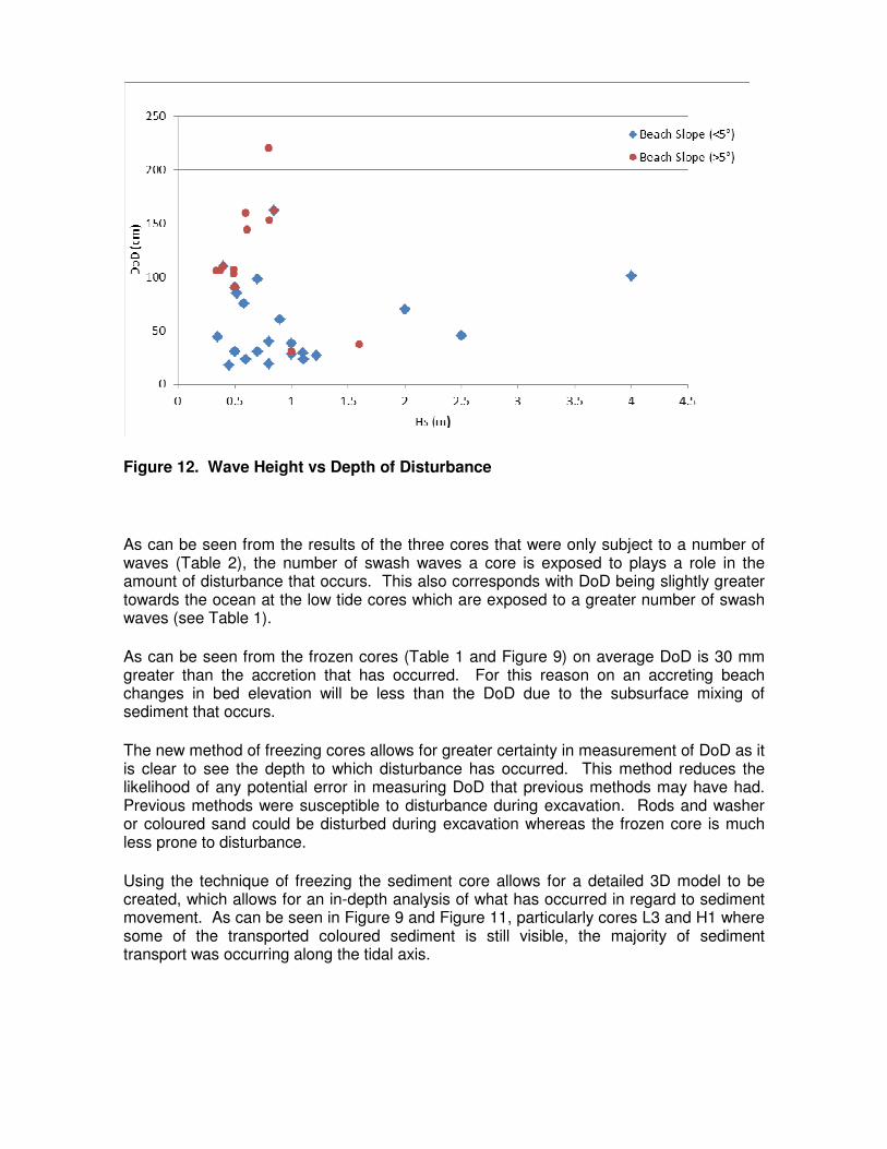
Figure 12. Wave Height vs Depth of Disturbance

As can be seen from the results of the three cores that were only subject to a number of waves (Table 2), the number of swash waves a core is exposed to plays a role in the amount of disturbance that occurs. This also corresponds with DoD being slightly greater towards the ocean at the low tide cores which are exposed to a greater number of swash waves (see Table 1).

As can be seen from the frozen cores (Table 1 and Figure 9) on average DoD is 30 mm greater than the accretion that has occurred. For this reason on an accreting beach changes in bed elevation will be less than the DoD due to the subsurface mixing of sediment that occurs.

The new method of freezing cores allows for greater certainty in measurement of DoD as it is clear to see the depth to which disturbance has occurred. This method reduces the likelihood of any potential error in measuring DoD that previous methods may have had. Previous methods were susceptible to disturbance during excavation. Rods and washer or coloured sand could be disturbed during excavation whereas the frozen core is much less prone to disturbance.

Using the technique of freezing the sediment core allows for a detailed 3D model to be created, which allows for an in-depth analysis of what has occurred in regard to sediment movement. As can be seen in Figure 9 and Figure 11, particularly cores L3 and H1 where some of the transported coloured sediment is still visible, the majority of sediment transport was occurring along the tidal axis.

Table 3. Summary of Depth of Disturbance Results

Authors Place - Year Hbs (m)

Tz (s)

Beach Slope

(°)

Measured DoD (mm)

1.86Hbstan β (Ferreria et al. (1998)

DoD/Hs

Greenwood and Hale 1980

Kouchibouguac Bay 76

2 6.5 - 70 - 0.35

Sunamura and Kraus 1985

Aijgaura 78 1 9 0.6 38 19 0.04

Aijgaura 79 1.1 6.5 0.6 29 21 0.03

Shimokita 79 0.6 4.9 1.2 23 23 0.04

Hirono 80 1.6 8.7 5.7 37 297 0.02

Hirono 80 1 8.4 5.7 30 186 0.03

Orai 80 1 10.2 0.6 28 19 0.03

Orai 81 1.11 6.1 0.6 23 22 0.02

Orai 82 0.8 75 1.2 19 31 0.02

Sherman et al 1994 Fire Island 92 1.22 - - 27 - 0.22

Ciavola et al 1997 Culata 93 0.37 5.8 6.3 106 76 0.29

Culata 93 0.34 5.1 6.3 106 70 0.31

Culata 93 0.37 5.1 6.3 106 76 0.29

Garrao 93 0.49 5.4 5.7 103 91 0.21

Faro 96 0.8 7 7.9 220 206 0.28

Ferreria et al 1998 Quarteira 96 0.49 - 6.3 107 101 0.22

Quarteira 97 0.6 - 5.7 160 111 0.27

Quarteira 97 0.81 - 5.7 153 150 0.19

Quarteira 97 0.61 - 6.8 144 135 0.24

Faro 97 0.85 - 7.9 162 219 0.19

Anfuso et al 2000 Rota 96 0.52 10 3.4 85 57 0.16

Rota 97 0.58 11 3.4 75 64 0.13

La Ballena 97 0.35 4.5 2.3 44 26 0.13

Tres Piedras 97

0.7 10 1.2 30 27 0.04

Tres Piedras 97

0.45 10 1.2 18 18 0.04

Tres Piedras 97

0.8 12 1.2 40 31 0.05

Anfuso et al 2003 Aguadulce 97 0.9 12 2.8 60 82 0.07

La Barrosa 97 0.5 9 1.7 30 28 0.06

Anfuso and Ruiz 2004

Faro 02 0.5 4 1.2 30 19 0.06

Faro 02 0.5 4 6.3 90 103 0.18

Ciavola et al 2005 Beach Models – Wave Flume 04

2.5- 4.0

6.5 -

9.0

1.1 - 3.0

45 - 101 - 0.2

Sani et al 2009 Delaware 06 0.4 9 110 118 0.22

Brook 2010 Southport 05 0.7 4.3 4.3 98 98 0.14

Combined with a SWAN wave model of the study area and further calibration of depth of disturbance to wave height, it will be possible to instantaneously estimate DoD on beaches where an offshore wave buoys exist.

Using the relationship determined earlier for converting offshore wave height to nearshore wave height a relationship for offshore wave height to DoD was established based on the data obtained in this experiment. To confidently establish this relationship, further experiments over varying wave conditions would be required. However from the results it shows that using a SWAN model to convert the offshore wave height it would be possible to instantaneously estimate the DoD occurring on a given beach from the readily available DERM wave data.

Based on the dominant relationship of Hbs to DoD for a known beach slope, DoD was plotted for varying offshore wave heights (see Figure 13). A second order polynomial was fitted to the data.

Zm = -13.342Hof2 + 118.57Hof + 4.1816

Where Zm is the depth of disturbance and Hof is the offshore significant wave height at the DERM wave buoy.

0

20

40

60

80

100

120

140

160

180

200

220

240

260

280

300

0 0.2 0.4 0.6 0.8 1 1.2 1.4 1.6 1.8 2 2.2 2.4 2.6 2.8 3 3.2 3.4 3.6 3.8 4 4.2 4.4 4.6 4.8 5

Offshore Hs (m)

De

pth

of

Dis

turb

an

ce

(m

m)

Figure 13. Offshore Significant Wave Height vs Predicted Depth of Disturbance

The new technique has shown that by freezing the cores, DoD can be determined more accurately and with more certainly than previous methods. Creating a 3D model allows for detailed analysis of the DoD results.

Experimental results showed that although in the past DoD has primarily been related to significant wave height the large variation in this relationship shows other factors are important. The strong correlation between DoD being related to both beach slope and wave height clearly shows beach slope is a critical factor. Given the coarser the beach sediment the steeper the beach formed (Shepard 1963), then in turn sediment grain size must be influential on DoD.

By creating a SWAN model to relate offshore wave height to nearshore wave height, it will be possible to relate DoD to offshore wave height for a given beach with sufficient calibration. With readily available offshore wave data this will lead to easy predictions of DoD for a given beach. This could be extremely valuable for planning beach nourishment projects where offshore wave data is readily available. On the Gold Coast for example offshore wave buoys instantaneously monitor wave conditions at both ends of the coast. This could be used to help schedule dredging and sand bypassing operations for beach nourishment.

REFERENCES

Anfuso, G., Gracia, F.J., Andres,J., Sanchez,F., Del rio, L., Lopez, F., (2000). “Depth of disturbance in mesotidal beaches during a single tidal cycle.” Journal of Coastal Research, 10(2) 297-305

Anfuso, G., Benavente, J., Del Rio, L., Castiglione, E., Ventorre, M., (2003). “Sand transport and disturbance depth during a single tidal cycle in a dissipative beach: La Barrosa (SW Spain).” Proc. 3

rd IAHR, Symp. Riv., Coast. Estuar. Morphod. 2, 1176 -1186

Anfuso, G., Ruiz, N., (2004). “Morphodynamic of a mesotidal, low tide terrace exposed beach (Faro,Sout Protugal)” Cienc. Mar., 30 (4), 575 - 584

Anfuso, G. (2005). "Sediment-activation depth values for gentle and steep beaches." Marine Geology 220(1-4): 101-112.

Butt, T., Russell, P.G.L., Turner, I.L (2001). “The influence of swash infiltration-exfiltration on beach face sediment transport: onshore or offshore?” Coastal Engineering 42(1): 35-52.

Ciavola, P., Taborda, R., Ferreira, O., Alveirinho Dias, J. (1997). “Field observations of sand-mixing depths on steep beaches.” Marine Geology 141(1-4): 147-156.

Colin Cameron, A. and Windemijer, F.A.G.(1997). “An R-squared measure of goodness of fit for some common nonlinear regression models.” Journal of Econometrics 77(3): 329-342.

DHL, 1970. “Gold Coast, Queensland, Australia - Coastal Erosion and Related Problems.” Delft Hydraulics Laboratory, Netherlands, Report R257.

DHL, 1992. “Southern Gold Coast Littoral Sand Supply.” Delft Hydraulics Laboratory, The Netherlands, Report H85.

Ferreira, O., Bairros, M., Pereira, H., Ciavola, P., Dias, J.A., (1998). “Mixing depth levels and distribution on steep foreshores” Journal of Coastal Research (Special Issue 26): 292-296.

Ferreira, O., Ciavola, P., Taborda, R., Bairros, M., Dias, J.A., (2000). Sediment mixing depth determination for steep and gentle foreshores. Journal of Coastal Research 16 (3), 830– 839.

Greenwood, B. and Hale, P. (1980). “Depth of activity, sediment flux and morphological change in a barred nearshore environment.” Geology and Surveying: 88-109.

Holman, R. and Sallenger, A. (1985). “Set up and swash on a natural beach.” Journal of Geophysical Research (90): 945-953.

Jackson, D. and Malvarez, G. (2002). “A new, high-resolution ‘depth of disturbance’ instrument (SAM) for use in the surf zone.” Journal of Coastal Research – Special Issue 36: 406-413.

King (1051). “Depth of Disturbance of sand on sea beaches by waves.” Journal of Sediment Petrol 21: 131-140.

Kraus, N. (1985). “Field experiments on vertical mixing of sand in the surf zone.” Journal of Sediment Petrol 53: 3-14.

Nielsen, P. (1989) – “Measuring waves with pressure transducers – Discussion” Coastal Engineering Vol 12 Issue 4 381-385.

Sani, S., Jackson, N., Nordstorm, K.F. (2009). “Depth of activation on a mixed sediment beach.” Coastal Engineering 56(7): 788-791.

Shepard, F.P. (1963). Submarine Geology. 2nd

ed. New York: Harper Row.

Sherman, D., Nordstrom, K.F., Jackson, N.L., Allen, J.R., (1994). “Sediment mixing-depths on a low-energy reflective beach.” Journal of Coastal Research 10(20) 297-305.

Sunamura, T. and Kraus, N.C. (1985). “Prediction of average mixing depth of sediment in the surf zone.” Marine Geology 62(1-2_: 1-12.

Svendsen, I.A. and Putrevu U. (1996). “Surf zone hydrodynamics” Advances in Coastal and Ocean Engineering, (World Scientific (1996)) pp 1-78.

Williams, A.T. (1971). “An analysis of some factors involved in the depth of disturbance of beach sand by waves.” Marine Geology 11(3): 145-158.