Comput Mech (2014) 54:407–424DOI 10.1007/s00466-014-0994-4

ORIGINAL PAPER

A finite element model for coupled 3D transient electromagneticand structural dynamics problems

Shu Guo · Somnath Ghosh

Received: 13 November 2013 / Accepted: 30 January 2014 / Published online: 21 February 2014© Springer-Verlag Berlin Heidelberg 2014

Abstract This paper develops a framework for couplingtransient electromagnetic (EM) and dynamic mechanical(ME) fields to predict the evolution of electrical and mag-netic fields and their fluxes in a vibrating substrate undergo-ing finite deformation. To achieve coupling between fieldsthe governing equations are solved in the time domain. ALagrangian description is invoked, in which the couplingscheme maps Maxwell’s equations from spatial to mater-ial coordinates in the reference configuration. Physical vari-ables in the Maxwell’s equations are written in terms of ascalar potential and vector potentials. Non-uniqueness in thereduced set of equations is overcome through the introduc-tion of a gauge condition. Selected features of the code arevalidated using existing solutions in the literature, as wellas comparison with results of simulations with commercialsoftware. Subsequently, two coupled simulations featuringEM fields excited by steady-state and transient electric cur-rent source in dynamically vibrating conducting media arestudied.

Keywords Coupled multiphysics · Dynamic finitedeformation · Transient electromagnetic · Time-domainfinite element method

1 Introduction

The recent times have seen a high interest in multifunctionalstructures that are governed by multiphysics principles suchas mechanical and electromagnetic relations. These struc-tures can be components of small unmanned airborne vehi-

S. Guo · S. Ghosh (B)Department of Civil Engineering, Johns Hopkins University,Baltimore, MD 21218, USAe-mail: sghosh20@jhu.edu

cles (UAVs), active skins of aircraft, meta-materials for opti-cal and communication systems etc. These devices can havemultiple phases in the form of embedded conductors and/orreinforcing fibers in the matrix or substrate. Conductors canalso serve as reinforcing phases for structural integrity andstability. Standard EM devices such as antennae and sen-sors have been traditionally based on stiff structures and aretypically designed for transmission of EM waves alone with-out deformation considerations. In the recent years, flexibledevices in energy, sensing, memory, and electromagneticssuch as high mobility and stretchable electronics, elastomer-based EM devices, optical dielectric resonator antennas etc.are increasingly gaining importance [1,2]. In most of thesedevices the mechanical fields in the structure have significanteffect on the EM signals. Discussions on utility and require-ments of load-bearing antenna have been made in [3,4]. Loadbearing antennae are subjected to mechanical vibrations,which have frequencies that are considerably different fromthose for the EM field. For piezoelectric devices, couplingbetween the fields happens naturally since the piezoelectricmaterial is able to convert mechanical energy to electricalenergy and vice-versa. Other examples of ME–EM couplinginclude electromagnetic forming (EMF), where EM forcesare utilized to deform a solid body in the forming process.There is a need for robust, coupled multiphysics computa-tional models and codes for meaningful design of multifunc-tional structures and devices.

Modeling the evolution of EM fields in a moving deforma-ble media is a challenging problem. Only a limited numberof coupled computational models are available in the litera-ture. Finite element analysis of the EM problems for signaltransmission in antennas has been mostly carried out in thefrequency domain [5]. However, frequency domain compu-tations are not suitable when coupled with finite deformationanalysis. Novel descriptions of hp-adaptive finite elements

123

408 Comput Mech (2014) 54:407–424

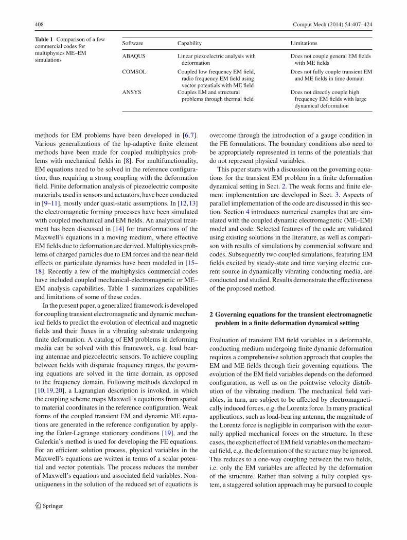
Table 1 Comparison of a fewcommercial codes formultiphysics ME–EMsimulations

Software Capability Limitations

ABAQUS Linear piezoelectric analysis withdeformation

Does not couple general EM fieldswith ME fields

COMSOL Coupled low frequency EM field,radio frequency EM field usingvector potentials with ME field

Does not fully couple transient EMand ME fields in time domain

ANSYS Couples EM and structuralproblems through thermal field

Does not directly couple highfrequency EM fields with largedynamical deformation

methods for EM problems have been developed in [6,7].Various generalizations of the hp-adaptive finite elementmethods have been made for coupled multiphysics prob-lems with mechanical fields in [8]. For multifunctionality,EM equations need to be solved in the reference configura-tion, thus requiring a strong coupling with the deformationfield. Finite deformation analysis of piezoelectric compositematerials, used in sensors and actuators, have been conductedin [9–11], mostly under quasi-static assumptions. In [12,13]the electromagnetic forming processes have been simulatedwith coupled mechanical and EM fields. An analytical treat-ment has been discussed in [14] for transformations of theMaxwell’s equations in a moving medium, where effectiveEM fields due to deformation are derived. Multiphysics prob-lems of charged particles due to EM forces and the near-fieldeffects on particulate dynamics have been modeled in [15–18]. Recently a few of the multiphysics commercial codeshave included coupled mechanical-electromagnetic or ME–EM analysis capabilities. Table 1 summarizes capabilitiesand limitations of some of these codes.

In the present paper, a generalized framework is developedfor coupling transient electromagnetic and dynamic mechan-ical fields to predict the evolution of electrical and magneticfields and their fluxes in a vibrating substrate undergoingfinite deformation. A catalog of EM problems in deformingmedia can be solved with this framework, e.g. load bear-ing antennae and piezoelectric sensors. To achieve couplingbetween fields with disparate frequency ranges, the govern-ing equations are solved in the time domain, as opposedto the frequency domain. Following methods developed in[10,19,20], a Lagrangian description is invoked, in whichthe coupling scheme maps Maxwell’s equations from spatialto material coordinates in the reference configuration. Weakforms of the coupled transient EM and dynamic ME equa-tions are generated in the reference configuration by apply-ing the Euler-Lagrange stationary conditions [19], and theGalerkin’s method is used for developing the FE equations.For an efficient solution process, physical variables in theMaxwell’s equations are written in terms of a scalar poten-tial and vector potentials. The process reduces the numberof Maxwell’s equations and associated field variables. Non-uniqueness in the solution of the reduced set of equations is

overcome through the introduction of a gauge condition inthe FE formulations. The boundary conditions also need tobe appropriately represented in terms of the potentials thatdo not represent physical variables.

This paper starts with a discussion on the governing equa-tions for the transient EM problem in a finite deformationdynamical setting in Sect. 2. The weak forms and finite ele-ment implementation are developed in Sect. 3. Aspects ofparallel implementation of the code are discussed in this sec-tion. Section 4 introduces numerical examples that are sim-ulated with the coupled dynamic electromagnetic (ME–EM)model and code. Selected features of the code are validatedusing existing solutions in the literature, as well as compari-son with results of simulations by commercial software andcodes. Subsequently two coupled simulations, featuring EMfields excited by steady-state and time varying electric cur-rent source in dynamically vibrating conducting media, areconducted and studied. Results demonstrate the effectivenessof the proposed method.

2 Governing equations for the transient electromagneticproblem in a finite deformation dynamical setting

Evaluation of transient EM field variables in a deformable,conducting medium undergoing finite dynamic deformationrequires a comprehensive solution approach that couples theEM and ME fields through their governing equations. Theevolution of the EM field variables depends on the deformedconfiguration, as well as on the pointwise velocity distrib-ution of the vibrating medium. The mechanical field vari-ables, in turn, are subject to be affected by electromagneti-cally induced forces, e.g. the Lorentz force. In many practicalapplications, such as load-bearing antenna, the magnitude ofthe Lorentz force is negligible in comparison with the exter-nally applied mechanical forces on the structure. In thesecases, the explicit effect of EM field variables on the mechani-cal field, e.g. the deformation of the structure may be ignored.This reduces to a one-way coupling between the two fields,i.e. only the EM variables are affected by the deformationof the structure. Rather than solving a fully coupled sys-tem, a staggered solution approach may be pursued to couple

123

Comput Mech (2014) 54:407–424 409

the dynamical response with the EM field in this work. Thegoverning equations for the mechanical and electromagneticproblems are discussed next.

2.1 Governing equations for the finite deformationdynamics problem

The mechanical response of the conducting medium is mod-eled using governing equations for a hyperelastic materialundergoing finite deformation under dynamic loading con-ditions. In a Lagrangian formulation, the reference config-uration Ω0(=Ω(t0)) at a time t0 is expressed in terms ofthe material coordinates X I , I = 1, 2, 3, while the cur-rent configuration Ω(t) at time t is represented by the cur-rent coordinates xi , i = 1, 2, 3. The deformation of thebody is expressed using the single-valued mapping functionxi = ϕi (X J , t). Correspondingly, the Cartesian componentsof the displacement vector in the material coordinates areexpressed as: ui (X J , t) = xi −δi J X J . The constitutive rela-tion for the hyperelastic material at finite strains is assumed tobe neo-Hookean, for which the strain energy density functionW is expressed in terms of kinematics variables as:

W = 1

2λ(ln J )2 − μ ln J + 1

2μ (CI I − 3) (1)

where λ and μ are Lame constants, and CI J (= ∂xk∂X I

∂xk∂X J

)

is the right Cauchy-Green deformation tensor. The positive-valued Jacobian J , which determines admissible deforma-tion mapping, is defined in terms of the deformation gradienttensor Fi J as:

J = det (Fi J ) > 0 where Fi J = ∂xi

∂X J(2)

The stress–strain relation for finite strains is derived from theenergy density expression in (1) as:

SI J = J∂X J

∂xm

∂X I

∂xnσmn

= 2∂W

∂CI J= λ ln J C−1

I J + μ(δI J − C−1I J ) (3)

where SI J and σi j are components of the second Piola–Kirchhoff and Cauchy stress tensors respectively. A secondhyperelastic logarithmic stretch model [21] is also imple-mented in this work, where the strain energy density functionis defined in terms of principal strain εm as:

W = 1

2λ

3∑

m=1

(εm)2 + μ

3∑

m=1

(ε2m) (4)

where εm = log(λm), λm being the square root of the prin-cipal values of CI J . The principal values τm of Kirchhoff

stress τi j are expressed in term of W as:

τm = ∂W

∂εm= λ

(3∑

m=1

εm

)+ 2μεm (5)

Finally from Eq. (5), the second Piola–Kirchhoff is obtainedas

SI J = ∂xI

∂xkτkl∂xJ

∂xl

= ∂xI

∂xk

∑

m

[λ

(3∑

m=1

εm

)+ 2μεm

]q(m)k q(m)l

∂xJ

∂xl(6)

where q(m)i are direction cosines of principal direction m andcomponent direction i .

The equilibrium equation in finite deformation theory isexpressed as:

∂Pi J

∂X J+ ρ0bi = ρ0ui (7)

where Pi J (= ∂xi∂X K

SK J ) is the first Piola–Kirchhoff stress,ρ0 is the density in the reference configuration and bi is thebody force per unit mass.

2.2 Governing equations for the electromagnetic problemin current and reference configurations

The governing equations for the EM problem is based on theconventional Maxwell’s equations for a conducting medium.In the current configuration, these equations are expressed interms of the current coordinates xi (t) as:

di ,i = qe Gauss’ law of electricity (8a)

bi ,i = 0 Gauss’ law of magnetism (8b)

εi jkek, j = −∂bi

∂tFaraday’s law of magnetism (8c)

εi jkhk, j = ∂di

∂t+ j f

i Ampere’s law (8d)

Here di represents the Cartesian components of the electricaldisplacement field vector, qe is the free charge density, bi arethe components of the magnetic induction field vector, ei isthe electric field, hi is the magnetic field strength, and j f

i isthe free charge current defined as:

j fi � j c

i + qexi . (9)

where j ci is conducting current and εi jk is the Levi-Civita

permutation symbol. The constitutive laws for an isotropicmaterial in the current configuration, in the absence of mag-netization and polarization, are given as:

di = εei , hi = 1

μbi , j c

i = σ(ei + εi jk x j bk) (10)

123

410 Comput Mech (2014) 54:407–424

where the permittivity ε, permeability μ and conductivity σare material constants.

For coupling with the set of mechanical field equationsfor the deforming medium, it is necessary to represent theMaxwell’s equations in a reference material configurationΩ0. The Lagrangian description in Sect. 2.1, provides a con-sistent platform for solving the coupled dynamic-EM prob-lem. The transformation from current to reference configu-ration requires the flux derivative of any field vector Vi interms of the local time derivatives as [22]:

∗Vi= ∂Vi

∂t+ Vj , j xi + (Vi xk − Vk xi ),k (11)

satisfying the integral form of the flux derivative relation:

d

dt

∫

∂Ω

Vi ni ds =∫

∂Ω

∗Vj n j ds. (12)

Here xi corresponds to the velocity field and (),i corre-sponds to the spatial derivative. Derivation of the relation(11) utilizes the Nanson’s formula of surface area transfor-mation between the current and the reference configurations,expressed as:

ni ds = J X J ,i NJ d S (13)

where ni ds and NI d S are differential area vectors, ds and d Sare surface areas, and ni and NI are surface normals in thecurrent and reference configurations respectively. The fluxderivative of the electric displacement di is obtained fromEq. (11) as:

∂di

∂t= ∗

di −(di xk − dk xi ),k −d j , j xi (14)

Now

εi jk∂

∂x jhk = εik j

∂

∂xkh j = −εi jk

∂

∂xkh j and

(di xk − dk xi ),k = (δimδkn − δkmδin)(dm xn),k

= ε j ikε jmn(dm xn),k (15)

Substituting Eq. (8a) and (14) in Eq. (8d) and rearrangingindices yields the relation:

εik j [h j + ε jmn(dm xn)],k = ∗di + j f

i − qexi (16)

where, the identity∑3

i=1 εi jkεimn = δimδkn − δkmδin isused. Equation (16) is transformed to the reference configu-ration by integrating it over an arbitrary surface area in thecurrent configuration, applying the Kelvin–Stokes’ theorem,and mapping to the reference configuration using Eq. (13) toyield:

∮

C[hi + εimn(dm xn)]xi ,J d X J

=∫

∂Ω0

(∗

d j + j fj − qex j )J X I , j NI d S0 (17)

where C corresponds to the contour line around the surface.The reference configuration electric displacement, magneticfield and free charge current in the conductor are defined interms of those in the current configuration as:

DI � J X I , j d j (18a)

HJ � [hi + εimn(dm xn)]xi ,J (18b)

J cI � J X I , j j c

j (18c)

With these reference configuration field variables, Eq. (17)is reduced to the configuration-invariant relation:

εI J K HK ,J = d

dtDI + J c

I (19)

The permutation operator εI J K in the reference configurationis related to εi jk as:

εI J K = J−1εi jk xi ,I x j ,J xk,K or inversely

εi jk = JεI J K X I ,i X J , j X K ,k (20)

In a similar manner, substituting bi in Eq. (11) and usingEqs. (8b) and (8c) results in a relation between the magneticinduction field bi and the electric field ei as:

εi jkek, j = (bi xk − bk xi ),k − ∗bi or (21a)

εi jk[e j − ε jmn(bm xn)],k = − ∗bi (21b)

Integrating Eq. (21b) over a surface area in the current con-figuration, applying the Kelvin–Stokes’ theorem, and subse-quently transforming into the reference configuration yields:

∮

C[e j − ε jmn(dm xn)]x j ,I d X I = −

∫

∂Ω0

∗b j J X J ,i NJ d S0

(22)

The electric and magnetic induction fields in the referenceconfiguration are defined as:

EI � [e j − ε jmn(bm xn)]x j ,I (23a)

BJ � J X J ,i bi (23b)

The Faraday’s Eq. (8c) in the reference configuration is thenexpressed as:

εI J K EK ,J = − d

dtBI (24)

For the Gauss’ law of electricity in Eq. (8a), the transforma-tion is achieved by integrating over the volume and applying

123

Comput Mech (2014) 54:407–424 411

the divergence theorem, along with the Nanson’s formula ofsurface transformation, to yield:

∫

∂Ω

di ni ds =∫

Ω

qedv ⇒∫

∂Ω0

di J X J,i NJ d S =∫

Ω0

qe JdV

(25)

By defining the charge density in the reference configurationas Qe = Jqe, Eq. (8a) in the reference configuration becomes

DI ,I = Qe (26)

Following the same mapping procedure, the Gauss’ law ofmagnetism of Eq. (8b) is transformed to:

BJ ,J = 0 (27)

In summary, the four Maxwell’s equations in the referenceconfiguration are written in the indicial and vector forms as:

Indicial Notations Vector Notations

DI ,I = Qe ∇X · D = Qe (28)

BJ ,J = 0 ∇X · B = 0 (29)

εI J K∂

∂X JEK = − d

dtBI ∇X × E = − d

dtB (30)

εI J K∂

∂X JHK = d

dtDI + J c

I ∇X × H= d

dtD+Jc (31)

Constitutive relations in the reference configuration, relat-ing DI and EI , BI and HI , as well as J c

I and EI and BI , arenonlinear due to coupling with the deformation fields. Thefollowing steps are used to determine the set of constitutiverelations. Using the inverse of Eq. (23b), i.e.

b j = J−1x j ,I BI (32)

and the velocity relations

xi = −xi ,K∂X K

∂tor inversely

∂X K

∂t= −X K ,i xi (33)

in Eq. (23a), its inverse is obtained as:

ei = E J X J ,i +εimn(bm xn) = E J X J ,i

−X J ,i (εimn J−1xi ,J xm,L xn,K )

(∂X K

∂tBL

)

= X J ,i

[E J + εJ K L

(∂X K

∂tBL

)](34)

Substituting Eqs. (18a) and (10) in Eq. (34) yields the con-stitutive relation for the electrical displacement field in the

reference configuration as:

DI = εJ X I , j X J , j

[E J + εJ K L

(∂X K

∂tBL

)]

= εJC−1I J

[E J + εJ K L

(∂X K

∂tBL

)](35)

In a similar manner, the magnetic field strength in both con-figurations are related as:

hi = HJ X J,i − εimn(dm xn) = HJ X J ,i

+X J,i (εimn J−1xi ,J xm,L xn,K )

(∂X K

∂tDL

)

= X J ,i

[HJ −

(εJ K L(

∂X K

∂tDL

)](36)

Substituting Eqs. (32) and (35) in Eq. (36) results in the con-stitutive relation for magnetic field strength in the referenceconfiguration as:

HJ = hi xi ,J +εJ K L∂X K

∂tDL = 1

μJ−1xi ,M xi ,J BM

+εJ K L∂X K

∂t

{εJC−1

L N

[EN + εN P Q

(∂X P

∂tBQ

)]}

= 1

μJ−1CM J BM + εJ K L

∂X K

∂t

{εJC−1

L N

[EN

+εN P Q

(∂X P

∂tBQ

)]}(37)

Finally, incorporating Eq. (18c) and Eq. (34) in Eq. (10) pro-vides the constitutive relation for the current in the referenceconfiguration as:

J cI = σ JC−1

I J E J (38)

2.3 Scalar and vector potentials in current and referenceconfigurations

For effective solution of the Maxwell’s equations, a scalarpotential ϕ for the electric field and a vector potential a forthe magnetic field in the current configuration have been pro-posed as primary variables, e.g. in [22]. This representation interms of the potential functions reduce the Maxwell’s equa-tions from four to two independent equations. Since the diver-gence of the magnetic induction vector b (in Eq. (8c)) is zero,the magnetic vector potential a can be derived using a vectoridentity, i.e.

∇ · b = ∇ · (∇ × a) = 0 �⇒ bi = εi jkak, j (39)

The Faraday’s law in Eq. (8c) may be rewritten in terms ofthe vector potential ai by substituting the expression for themagnetic field bi in Eq. (39), i.e.

εi jk(ek + ak), j = 0 (40)

123

412 Comput Mech (2014) 54:407–424

Since the curl of the gradient of any scalar field is a nullvector, the gradient of ϕ may be added to the LHS of Eq.(40) without changing the RHS, i.e.

εi jk(ek + ak + ϕ,k ), j = 0 (41)

The electric field may be then be expressed using mixedpotentials as:

ek = −ϕ,k −ak (42)

For electrostatic problems, the electric potential ϕ corre-sponds to the ratio of potential energy to charge. Introductionof these two potentials in the Gauss’s law for magnetism inEq. (8b) and the Faraday’s law in Eq. (8c) results in identities.The other two Maxwell’s equations are reformulated usingthe mixed potentials as:

∇2ϕ + ∂

∂t(ai ,i ) = −qe (43a)

(∇2ai − με

∂2ai

∂t2

)−

(ak,k +με∂ϕ

∂t

),i = −μji (43b)

The corresponding reduced forms of the Maxwell’s equa-tions in the reference configuration requires consistent formsof both the potentials in this configuration. Defining trans-formation functions as:

AK = ai xi ,K ⇐⇒ ai = AK X K ,i and (44a)

Φ = ϕ − dxi

dtai ⇐⇒ ϕ = Φ − ∂X I

∂tAI (44b)

Scalar and vector potentials defined in the reference config-uration follow relations similar to those in the current con-figuration, i.e.

EI = −Φ,I −∂AI

∂t(45a)

BI = εI J K AK ,J (45b)

Details of the derivation of Eqs. (44a), (44b) and proofs ofEqs. (45a) and (45b) are given in [22]. Substituting Eqs. (45a)and (45b) in Eq. (28) and Eq. (31) results in the two governingequations(εJC−1

I J E J

),I = Qe (46a)

εI J K

(1

μJCK LεL M N AN ,M + εK P Q

∂X P

∂tεJC−1

Q R ER

),J

= d

dtεJC−1

I P EP + σ JC−1I Q

(−Φ,Q − AQ)

(46b)

where E I is defined as:

E I = EI + εI J K∂X J

∂tBK

= −Φ,I − AI + εI J K∂X J

∂tεK M N AN ,M (47)

2.4 Constraint Gauge condition for solution uniqueness

While the reduced representation of Maxwell’s equationsin terms of potentials is computationally advantageous, thesolution leads to non-uniqueness of the potentials and con-sequent singular tangent matrices for certain state of the EMfields. For example, the vector potential relation in Eq. (45b),can admit multiple solutions of the magnetic field due to thecondition:

∇·B =∇·(∇×A+∇Ψ )=0 �⇒ BI = εI J K AK ,J +ψ,I(48)

where AI is the vector potential component andΨ is any arbi-trary scalar potential in the reference configuration. This non-uniqueness will lead to a singular tangent stiffness matrixand consequent instability in the finite element model. Thishas been averted through the introduction of a variety of con-straint gauge conditions in the literature, viz. [11,23–26]. TheCoulomb gauge condition proposed in [11,24,26] is utilizedin the present work. It is stated as:

AI ,I = 0 (49)

This constraint forces the divergence of the vector potentialA to be zero. From the Helmholtz theorem [11], the vec-tor potential A can be decomposed into a divergence freerotational term and a curl-free irrotational term. Due to thevanishing irrotational part in Eq. (45b), the rotational termcontributes to the magnetic field BI and hence the Coulombgauge implies a restriction to the irrotational term. The con-straint gauge condition is implemented in the finite elementin a weak sense, using the penalty formulation following[11,24,26].

3 Weak forms and finite element implementation

Weak forms of the Lagrangian FEM formulation in the refer-ence configuration and their algorithmic implementation arediscussed in this section. The principle of virtual work is usedto obtain the weak form of the finite deformation dynamicsproblem in Eq. (7). The Hamilton’s principle of stationaryaction, in conjunction with the penalty formulation of thegauge constraint condition, is used to develop the weak formof the time dependent EM field. Appropriate boundary con-ditions are developed for both the mechanical and electro-magnetic problems in the reference configuration. The EMfields in the conducting medium are affected by the defor-mation and other mechanical field variables, while the EMfields have negligible effect on the mechanical fields in com-parison with the external loading. Hence, the Lorentz force

123

Comput Mech (2014) 54:407–424 413

is assumed to be negligible in this study. A one-directionalcoupling from the mechanical field to the EM field is thusconsidered, and a staggered solution scheme is implemented.A high performance parallel implementation of the coupledcode is also summarized in this section.

3.1 Weak form and boundary conditions of the finitedeformation dynamics problem

The principle of virtual work is developed by taking the innerproduct of Eq. (7) with the virtual displacement δui and inte-grating over volume in the reference configuration Ω0 as:

∫

Ω0

δui∂Pi J

∂X JdV0 +

∫

Ω0

δuiρ0bi dV0 =∫

Ω0

δuiρ0ui dV0 (50)

By applying the divergence theorem together with integrationby parts, the weak form reduces to∫

Ω0

δuiρ0ui dV0 +∫

Ω0

δFi J Pi J dV0 −∫

Ω0

δuiρ0bi dV0

−∫

∂Ω0

δui Pi J NJ d S0 = 0 (51)

Displacement and traction conditions on respective bound-aries in the reference configuration are expressed as:

UI = δI i ui = U 0I on Γu ∈ ∂Ω0

TI = Pi J NJ = T 0I on Γt ∈ ∂Ω0 (52)

Since the EM fields are assumed to have negligible effect onthe mechanical fields, the discrete form of Eq. (51), togetherwith the boundary conditions Eq. (52), are sufficient for solv-ing the deformation related fields of the substrate.

3.2 Weak form of the electromagnetic problem in thereference configuration

The weak form of the transient EM problem is derived usingthe Hamilton’s principle, [19,22]. It involves minimizationof the action functional S over the time range t1 − t2, definedin terms of the time-dependent Lagrangian density L in thereference domain, expressed as:

δS = δ

t2∫

t1

∫

Ω0

L dΩ0dt = 0 (53)

where the Lagrangian density in the reference and currentconfigurations, L and l respectively, are given as:

L = Jl =(ε

2ei ei − 1

2μb j b j + jkak − qϕ

)(54)

L may be expressed in terms of the scalar and vector poten-tials in the reference configuration using the expressions forei and bi in Eqs. (34) and (32), and substituting Eqs. (44a)and (44b) as:

L = εJ

2C−1

J K E J EK − J−1

2μ(CL M BL BM )+ JN AN − QΦ

(55)

Here EI , BI and E I are in terms of the scalar and vectorpotentials as given in Eqs. (45a), (45b) and (47).

Furthermore, the gauge condition in Eq. (49) is imple-mented using the penalty method to constrain the vectorpotentials following [11,24,26]. In this process, an additionalterm 1

p (∇ · A)2 is added to the Lagrangian density functionas:

L = εJ

2C−1

J K E J EK − J−1

2μ(CL M BL BM )

+JN AN − QΦ + 1

p(AP,P )

2 (56)

The term 1p is the penalty coefficient, for which p is generally

of the order of the electric permittivity ε.From Eq. (53), setting the variation of the action functional

S with respect to Φ and A to zero yields:

S,Φ [δΦ] =t2∫

t1

∫

Ω0

L ,Φ [δΦ]Ω0dt = 0 (57a)

S,A [δA] =t2∫

t1

∫

Ω0

L ,A [δA]Ω0dt = 0 (57b)

Since t1 and t2 are arbitrary, Eqs. (57a) and (57b) lead to:∫

Ω0

L ,Φ [δΦ]dV0 =∫

∂Ω0

NI

(εJC−1

I J E J δΦ)

d S0

−∫

Ω0

(εJC−1

I J E J − Q)δΦ,I dV0 = 0 (58a)

∫

Ω0

L ,A [δA]dV0 =∫

∂Ω0

NL(εK L M QMδAK )d S0

− 2

p

∫

∂Ω0

AR,R NK δAK d S0

+∫

Ω0

εS P R Q P∂

∂X RδASdV0 −

∫

Ω0

d

dtεJC−1

K J E J δAK dV0

−∫

Ω0

σ JC−1K I EI δAK dV0

123

414 Comput Mech (2014) 54:407–424

+ 2

p

∫

Ω0

AR,R δAK ,K dV0 = 0 (58b)

where the condensed term is expressed as:

QM = 1

μJCM N BN + εM N P

∂X N

∂tεJC−1

P Q EQ (59)

The weak forms in Eqs. (58a) and (58b) reduce to the strongforms in Eqs. (46a) and (46b). The scalar potential Φ andvector potentials A are the solutions of Eqs. (58a) and (58b).

3.2.1 Boundary conditions in terms of the potentials

Since potential functions are chosen as primary variablesin the solution of the EM field, the actual physical bound-ary conditions should be represented in terms of the scalarand vector potentials in the reference configuration. This isobtained by replacing the field variables with the potentialexpressions in the boundary term of the weak form Eq. (58a),i.e.,

∫

∂Ω0

NI

(ε0 JC−1

I J E J δΦ)

d S0

=∫

∂Ω0

NI

[ε0 JC−1

I J (−Φ,J − AJ

+ εJ L K∂X L

∂tεK M N AN ,M )δΦ

]d S0 (60)

where δΦ is the variation of Φ. For Dirichlet boundary con-ditions, e.g. applied voltage V = Φ = Φ0 in electrostaticproblem or for grounded boundary Φ = 0, δΦ = 0. Moreinvestigation is needed for parts of the boundary that are notgoverned by the Dirichlet boundary condition. For example,the boundary equation for the reference electric displacementfield DI in Eq. (35) is NI DI = ρs , where ρs is the surfacecharge density. This boundary condition can be implementedby substituting the value of surface charge density. Anotherboundary condition that can be expressed using Eq. (60) iscurrent injection, which is governed by the reference config-uration Ohm’s law Eq. (38). Assuming a fixed boundary inEq. (33) i.e. ∂X

∂t = 0, the boundary condition reduces to:∫

∂Ω0

NI

[εJC−1

I J (−Φ,J − AJ )]δΦd S0

=∫

∂Ω0

NI

[ε

JI

σ

]δΦd S0 (61)

This mixed form may be used to introduce the injected currentalong the surface normal.

The next step is to examine the boundary condition asso-ciated with the weak form in Eq. (58b). Following the same

procedure as before, the boundary terms corresponding tothe Dirichlet type condition reduce to:

∫

∂Ω0

NL

[εK L M

(1

μJCM N BN

+εM R P∂X R

∂tεJC−1

P Q EQ

)δAK

]d S0

− 2

p

∫

∂Ω0

AR,R NK δAkd S0 (62)

This includes boundary condition terms from both theMaxwell’s equation and the gauge condition. When valuesof AI are prescribed on the boundary, both terms in Eq. (62)go to zero. This simple boundary condition is associated withthe magnetic field B = 0 at the boundary. From Eq. (37) it isevident that for conditions other than the Dirichlet boundarycondition, Eq. (62) will hold when NI × HI is assigned tothe boundary.This result has the physical manifestation ofthe surface current.

To understand the effect of the first term in Eq. (62), afixed and undeformed boundary is assumed, thus yieldingthe relation:

∫

∂Ω0

NL

[εK L M

(1

μJCM N BN

)δAK

]d S0

=∫

∂Ω0

N ×[

1

μJ(∇ × A)

]δAd S0 (63)

Using a vector identity this may be rewritten as:∫

∂Ω0

N ×[

1

μJ(∇ × A)

]δAd S0 =

∫

∂Ω0

1

μJ[∇A(N · A)

−(N · ∇)A] δAd S0 (64)

Here N · A = An is the scalar component of the vec-tor potential A normal to the surface. ∇A is the Feynmansubscript notation, which implies that the subscripted gra-dient operates only on A. The other part is expressed as(N ·∇)A = ∂A

∂N , which corresponds to the flux, and hence theNeumann boundary condition in terms of A. If a tangentialmagnetic field is imposed on the boundary, there is no normalcomponent of An and the gauge condition term vanishes. Ifthe boundary is considered as a magnetic wall, the Neumannboundary condition in terms of A should be considered for afixed and undeformed boundary.

3.3 Finite element implementation of coupled ME–EMproblem

Numerical implementation of the weak forms and bound-ary conditions is conducted for the coupled problem using

123

Comput Mech (2014) 54:407–424 415

a staggered approach, where the dynamic displacement fieldis solved first followed by the electromagnetic problem. Thesemidiscretization method involving separation of variablesis used to represent the variables as discrete functions ofspace, yet continuous functions of time. For 8-noded brickelements, independent variables (displacements, scalar andvector potentials) of the coupled problem in each element eare interpolated as:

ue(X, t) ≈

8∑

α=1

ueα(t)N

eα(X),

Φe(X, t) ≈

8∑

α=1

Φeα(t)N

eα(X),

Ae(X, t) ≈

8∑

α=1

Aeα(t)N

eα(X) (65)

where N(X) are trilinear isoparametric shape functions ofthe brick element [27]. Note that both the mechanical andelectromagnetic field variables adopt the same finite elementmesh. The implicit time integration Newmark-beta method,which assumes constant average acceleration in each timestep [28], is implemented for integrating the dynamic prob-lems. Both the initial displacement and velocity are set to bezero, i.e. u(X, 0) = 0, u(X, 0) = 0. The backward Eulermethod is implemented for integrating the EM fields as:

Φe(X, tn) ≈

Φeα(tn)−Φe

α(tn−1)

ΔtN eα(X)

Ae(X, tn) ≈

Aeα(tn)− Ae

α(tn−1)

ΔtN eα(X) (66)

where Δt is time step that is determined from the higherfrequency response in the coupled problem. For the electro-magnetic field, Φ(X, 0) is set to be zero throughout domainexcept for certain boundary conditions. The vector potentialA and its rate A are obtained from the solution of the problemwith Φ(X, 0) = 0.

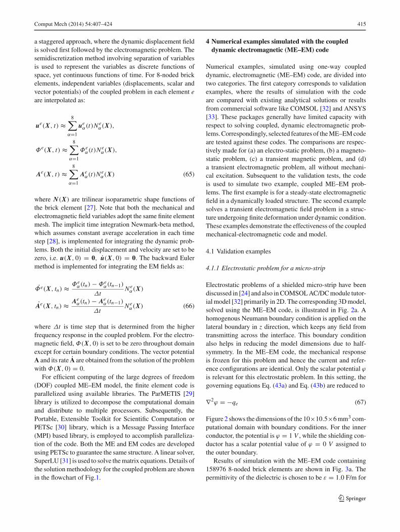
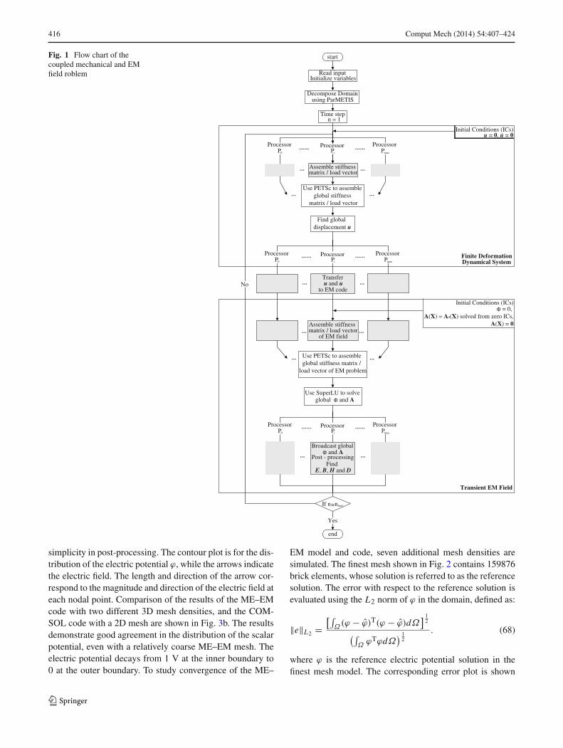
For efficient computing of the large degrees of freedom(DOF) coupled ME–EM model, the finite element code isparallelized using available libraries. The ParMETIS [29]library is utilized to decompose the computational domainand distribute to multiple processors. Subsequently, thePortable, Extensible Toolkit for Scientific Computation orPETSc [30] library, which is a Message Passing Interface(MPI) based library, is employed to accomplish paralleliza-tion of the code. Both the ME and EM codes are developedusing PETSc to guarantee the same structure. A linear solver,SuperLU [31] is used to solve the matrix equations. Details ofthe solution methodology for the coupled problem are shownin the flowchart of Fig.1.

4 Numerical examples simulated with the coupleddynamic electromagnetic (ME–EM) code

Numerical examples, simulated using one-way coupleddynamic, electromagnetic (ME–EM) code, are divided intotwo categories. The first category corresponds to validationexamples, where the results of simulation with the codeare compared with existing analytical solutions or resultsfrom commercial software like COMSOL [32] and ANSYS[33]. These packages generally have limited capacity withrespect to solving coupled, dynamic electromagnetic prob-lems. Correspondingly, selected features of the ME–EM codeare tested against these codes. The comparisons are respec-tively made for (a) an electro-static problem, (b) a magneto-static problem, (c) a transient magnetic problem, and (d)a transient electromagnetic problem, all without mechani-cal excitation. Subsequent to the validation tests, the codeis used to simulate two example, coupled ME–EM prob-lems. The first example is for a steady-state electromagneticfield in a dynamically loaded structure. The second examplesolves a transient electromagnetic field problem in a struc-ture undergoing finite deformation under dynamic condition.These examples demonstrate the effectiveness of the coupledmechanical-electromagnetic code and model.

4.1 Validation examples

4.1.1 Electrostatic problem for a micro-strip

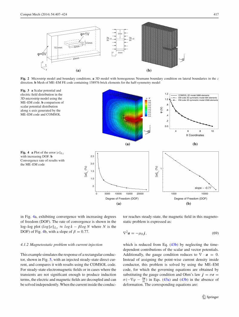
Electrostatic problems of a shielded micro-strip have beendiscussed in [24] and also in COMSOL AC/DC module tutor-ial model [32] primarily in 2D. The corresponding 3D model,solved using the ME–EM code, is illustrated in Fig. 2a. Ahomogenous Neumann boundary condition is applied on thelateral boundary in z direction, which keeps any field fromtransmitting across the interface. This boundary conditionalso helps in reducing the model dimensions due to half-symmetry. In the ME–EM code, the mechanical responseis frozen for this problem and hence the current and refer-ence configurations are identical. Only the scalar potential ϕis relevant for this electrostatic problem. In this setting, thegoverning equations Eq. (43a) and Eq. (43b) are reduced to

∇2ϕ = −qe (67)

Figure 2 shows the dimensions of the 10×10.5×6 mm3 com-putational domain with boundary conditions. For the innerconductor, the potential is ϕ = 1 V , while the shielding con-ductor has a scalar potential value of ϕ = 0 V assigned tothe outer boundary.

Results of simulation with the ME–EM code containing158976 8-noded brick elements are shown in Fig. 3a. Thepermittivity of the dielectric is chosen to be ε = 1.0 F/m for

123

416 Comput Mech (2014) 54:407–424

Fig. 1 Flow chart of thecoupled mechanical and EMfield roblem

start

Read inputInitialize variables

Decompose Domain using ParMETIS

Time stepn = 1

Use PETSc to assemble global stiffness matrix / load vector

Find global displacement u

Processor Pi

Processor Pmax

Processor P0

Assemble stiffness matrix / load vector

Transfer u and u

to EM code

Use PETSc to assemble global stiffness matrix /load vector of EM problem

Assemble stiffness matrix / load vector

of EM field

Use SuperLU to solve global and A

Broadcast global

Post - processingFind

If n=nmax

end

Yes

Finite Deformation Dynamical System

Initial Conditions (ICs)

Transient EM Field

Initial Conditions (ICs) = 0,

A(X) = A0(X) solved from zero ICs,A(X) = 0

Processor Pi

Processor Pmax

Processor P0

Processor Pi

Processor Pmax

Processor P0

and A

E, B, H and D

u = 0, u = 0˙

No

simplicity in post-processing. The contour plot is for the dis-tribution of the electric potential ϕ, while the arrows indicatethe electric field. The length and direction of the arrow cor-respond to the magnitude and direction of the electric field ateach nodal point. Comparison of the results of the ME–EMcode with two different 3D mesh densities, and the COM-SOL code with a 2D mesh are shown in Fig. 3b. The resultsdemonstrate good agreement in the distribution of the scalarpotential, even with a relatively coarse ME–EM mesh. Theelectric potential decays from 1 V at the inner boundary to0 at the outer boundary. To study convergence of the ME–

EM model and code, seven additional mesh densities aresimulated. The finest mesh shown in Fig. 2 contains 159876brick elements, whose solution is referred to as the referencesolution. The error with respect to the reference solution isevaluated using the L2 norm of ϕ in the domain, defined as:

‖e‖L2 =[∫Ω(ϕ − ϕ)T(ϕ − ϕ)dΩ

] 12

(∫ΩϕTϕdΩ

) 12

. (68)

where ϕ is the reference electric potential solution in thefinest mesh model. The corresponding error plot is shown

123

Comput Mech (2014) 54:407–424 417

(a) (b)

Fig. 2 Microstrip model and boundary conditions. a 3D model with homogenous Neumann boundary condition on lateral boundaries in the zdirection. b Mesh of ME–EM FE code containing 158976 brick elements for the half-symmetry model

Fig. 3 a Scalar potential andelectric field distribution in the3D microstrip model using theME–EM code. b comparison ofscalar potential distributionalong x-axis generated by theME–EM code and COMSOL

X

Z

Y

0.950.850.750.650.550.450.350.250.150.05

- V

(a)

X Coordinates

4 6 8 10

(V

)

0.0

.2

.4

.6

.8

1.0

1.2COMSOL 2D model 5888 elementsEM code 3D symmetric model 684 elementsEM code 3D symmetric model 2568 elements

(b)

Fig. 4 a Plot of the error |e‖L2

with increasing DOF. bConvergence rate of results withthe ME–EM code

Degree of Freedom (DOF)

0 5000 10000 15000 20000

|| e|| L

2

(%)

.5

1.0

1.5

2.0

2.5

(a)Degree of Freedom (DOF)

100001000

|| e|| L

2

(%)

1

slope ~ -0.77

(b)

in Fig. 4a, exhibiting convergence with increasing degreesof freedom (DOF). The rate of convergence is shown in thelog–log plot (log‖e‖L2 ≈ log k − βlog N where N is theDOF) of Fig. 4b, with a slope of β = 0.77.

4.1.2 Magnetostatic problem with current injection

This example simulates the response of a rectangular conduc-tor, shown in Fig. 5, with an injected steady-state direct cur-rent, and compares it with results using the COMSOL code.For steady-state electromagnetic fields or in cases where thetransients are not significant enough to produce inductionterms, the electric and magnetic fields are decoupled and canbe solved independently. When the current inside the conduc-

tor reaches steady-state, the magnetic field in this magneto-static problem is expressed as:

∇2a = −μ0 j , (69)

which is reduced from Eq. (43b) by neglecting the time-dependent contributions of the scalar and vector potentials.Additionally, the gauge condition reduces to ∇ · a = 0.Instead of assigning the point-wise current density insideconductor, this problem is solved by using the ME–EMcode, for which the governing equations are obtained bysubstituting the gauge condition and Ohm’s law j = σ e =σ(−∇ϕ − ∂a

∂t ) in Eqs. (43a) and (43b) in the absence ofdeformation. The corresponding equations are:

123

418 Comput Mech (2014) 54:407–424

XY

Z

6.5E-075.5E-074.5E-073.5E-072.5E-071.5E-075E-08

J=J0

(V)

=0V

0.25m

0.03m

0.05m

Fig. 5 FE model and mesh of the rectangular conductor showing cur-rent injection as well as electric potential distribution

∇2ϕ = −qe (70a)(

∇2ai − με∂2ai

∂t2

)−

(με∂ϕ

∂t

),i = μσ

(ϕ,i + ∂ai

∂t

)

(70b)

The current density in the conductor, in the right hand sideof Eq. (69), is imposed by the mixed boundary conditiongiven in Eq. (61), which assigns direct current injected fromone end. The conductor is grounded at the other end thatis manifested by setting the scalar potential to ϕ = 0. Thelateral sides are kept from any current flow by imposing aDirichlet boundary condition for the vector potential, i.e.a = 0. After the solution reaches the steady-state, the timedependent terms in Eq. (70a) and Eq. (70b) drop off. Bothscalar potential and vector potential are obtained as solu-tions. The results of ME–EM code are compared with thoseof COMSOL simulation in Fig.6, which shows ϕ at the mid-dle point of the surface where current is injected. The con-ducting material is considered to be aluminum, for whichthe permittivity is ε = 7.0832 × 10−11 F/m, the perme-ability is μ = 1.2567 × 10−6 H/m and the conductivity isσ = 37.8 × 106 S/m. Since the ME–EM code has transienteffects, results of the magnetostatic problem are achievedin the steady-state limit. Figure 6 shows that the resultsapproach the steady-state value faster with smaller time steps.This convergence trend is an indicator of stability of the ME–EM code.

4.1.3 Transient magnetic field problem

This example, discussed as case VM167 in the ANSYS verifi-cation manual [33], deals with the development of a transientmagnetic field in a static semi-infinite conductor. At start, thevector potential a in the conductor is zero, while at t = 0+ apulse in a is imposed on the boundary that generates a tran-sient magnetic field through the conductor. An eddy currentfield is rendered in the governing equations by removing thetime-dependent electric displacement field in Eq. (8d). Withthe constitutive relation in Eq. (10) and zero scalar potential,

Time (s)

0.000 .005 .010 .015 .020 .025

Ele

ctric

Fie

ld (

V/m

)

0

1e-7

2e-7

3e-7

4e-7

5e-7

6e-7

7e-7

Time Step = 0.005sTime Step = 0.002sTime Step = 0.001s

COMSOL (Magnetostatic)

Transient Zone

Fig. 6 Convergence of electric field with different time steps for mag-netostatic simulations by the ME–EM code

Z

X

Y

az=a0

a=0

3m

1m

0.4m

Fig. 7 Model of transient magnetic field problem in ME–EM code, thegradient mesh in y direction is kept same as that of in ANSYS

the governing equation after applying the gauge condition∇ · a = 0, reduces to:

∇2a − μσ∂a∂t

= 0, (71)

In ANSYS [33], the semi-infinite conductor is modeled in 2Das a thin wire with a graded mesh to better capture the signalnear the boundary where the pulse vector is applied. On theother end, a homogenous Dirichlet boundary condition a =A = 0 is applied. The corresponding computational domainwith graded mesh and boundary conditions for the 3D ME–EM model are depicted in Fig. 7. The material permeabilityis μ = 1.2567 × 10−6 H/m and the conductivity is σ =2.5 × 106 S/m. The transient vector potential and inducededdy current are monitored for the domain and reported fora point near the boundary where the pulse is imposed andtransient results are sensitive. A minimum time step of�t =0.0002 s is used in the simulations. Comparison of resultsby the ME–EM code and ANSYS are shown in Fig. 8a. Asobserved, the ME–EM code is able to capture and reproducethe transients simulated in ANSYS. An time-dependent error

123

Comput Mech (2014) 54:407–424 419

Fig. 8 Transient magnetic fieldsimulation results: a comparisonof vector potential in the zdirection between resultsgenerated by the ME–EM codeand ANSYS; b local error withevolving time

Time (s)

Az(

Wb/

m)

-.2

0.0

.2

.4

.6

.8

1.0

1.2

ANSYSME-EM code

(a)Time (s)

0.00 .05 .10 .15 .20 0.00 .05 .10 .15 .20

e (%

)

0

200

400

600

800

1000

1200

(b)

Fig. 9 a A slot embeddedconductor simulated in thetransient electromagnetic model.b Equivalent boundaryconditions on the conductordomain boundaries, thusavoiding free-space. c 3D FEmodel of the conductorimplemented in the ME–EMcode

w

air

µ0

µr

I

Steel Steel

conductor

(a)

z

n =− Iw

z

n = 0

w

Steel

z

n = 0

Steel

zan = 0

I

(b)

z

n = − Iw

a

aa

a

a zn = 0

on all the other sideboudaries

(c)

measure between the ME–EM and ANSYS results is defined

as e(t) =(

AAN SY Sz (t)−AE M

z (t))2

(AAN SY Sz (t))

2 × 100 % and plotted in Fig.

8b. While initial transient effects give rise to a few spikes inerror, it quickly subsides to zero with time.

4.1.4 Transient electromagnetic field problem

This final validation example explores a coupled, transientelectric and magnetic field problem using the ME–EM codeby simulating the transient response due to alternating current(AC) in a slot embedded conductor. The problem is intro-duced as a case study VM186 in the ANSYS verificationmanual [33], as well as in [34] for studying skin effect. Thegeometric model contains three parts, viz. air, conductor andsteel as shown in Fig. 9a. The conductor carries a current Iin the axial direction, perpendicular to its cross section. Thepermeability of the conductor is μ = 1.0 H/m while its con-ductivity is σ = 1.0 S/m. In the governing equations (72), thetotal measurable current is comprised of two parts, viz. (a) asource current I s determined by the scalar potential and (b)an eddy current Ie which is induced by the time derivativeof the vector potential. Since the scalar and vector potentialsare independent variables to be solved from Eq. (72), I s andIe are a-priori unknown.

∇2ϕ = −qe (72a)

∇2ai −(με∂ϕ

∂t

),i = μ

(σ ϕ, i︸︷︷︸

I s

+ σ∂ai

∂t︸︷︷︸Ie

)(72b)

The values of permeability for steel and the conductor mate-rial are significantly different, which makes it difficult totransmit magnetic flux across the interface. This assumptionrestricts the magnetic field to be within the conducting slotand hence only the conductor is simulated. A homogenousNeumann boundary condition, in terms of the gradient of thevector potential, is imposed on the interface between conduc-tor and steel to generate a magnetic wall as shown in Fig. 9b.The effect of EM fields in the free space or air is incorporatedthrough an equivalent boundary condition as given in [35].The computational domain is reduced to the conductor onlyby adding a Neumann boundary condition on the interfacebetween conductor and air as:

∂az

∂n= −μI

w(73)

Here w is the width of the cross-section as shown in Fig. 9b.The 3D computational model with boundary conditions aredepicted in Fig. 9b, c.

123

420 Comput Mech (2014) 54:407–424

Fig. 10 Comparison of theresults of transientelectromagnetic fieldsimulations by the ME–EMcode and ANSYS: a total andeddy current results simulation;b rate of convergence withdecreasing time steps

Time (s)

0 2 4 6

Cur

rent

Den

sity

(A

)

-80

-60

-40

-20

0

20

40

60

80

Eddy CurrentTotal CurrentTotal Current (ANSYS)Eddy Current (ANSYS)

(a)1/ t(s-1)

0 100 200 300 400 500 600

e (%

)

0.00

.02

.04

.06

.08

.10

(b)

Fig. 11 Schematic model of avibrating conductor withinjected current. The mechanicalloading is in z-direction, and thecurrent injects throughy-direction

Jy=J0 emt)

A=0 on SLu=0

0.25m

uz=u0 met)

0.03m

0.05m

XY

Z S1

S2

SL

Results of simulations, in terms of the total current andthe eddy current, by the ME–EM code and ANSYS are com-pared in Fig. 10a. While the results are generally in goodagreement, a small difference in the early time steps arisesfrom the initial conditions. To comprehend convergence ofthe ME–EM results with decreasing time-steps, simulationsare conducted with different time steps�t and an error mea-sure e is defined as:

e =∥∥∥∥

I M E−AM (�t)− I AN SY S

I AN SY S

∥∥∥∥ (74)

The error is plotted as a function of the inverse of the timestep, i.e. 1

�t . It reduces rapidly with decreasing time-steps asshown in Fig.10b.

4.2 Coupled mechanical and electromagnetic fieldsimulations

Subsequent to validation of the electromagnetic part of themodel and code, this section examines its abilities in pre-dicting the evolution of coupled, dynamic and transient elec-tromagnetic fields in multi-physics problems. Two examplesare specifically considered in this section. The first examinesthe effect of dynamic deformation on steady-state electro-magnetic fields in a conductor, while the second exampleexplores its effect on transient electromagnetic field vari-ables. For both examples, the conducting substrate is a rec-tangular plate as shown in Fig. 11. The logarithmic stretch

model is employed. The mechanical properties in Eq. (6)are given in terms of the Lame constants as λ = 40.4 GPaand μ = 26.9 GPa respectively, and the electromagneticproperties in Eqs. (10) are: ε = 7.0832 × 10−11 F/m,μ = 1.2567 × 10−6 H/m and σ = 37.8 × 106 S/m. Thedeforming conductor is fixed at one end, i.e. u = 0 on S2.The other end S1 is subjected to a z-direction sinusoidalexcitation uz(t) = u0 sin(ωmet). For the EM problem, thetop, bottom and side surfaces, designated as SL , are assignedhomogeneous Dirichlet boundary conditions for the vectorpotential i.e. A = 0 in the reference configuration. A currentJy(t) = J0 sin(ωemt) is injected into the fixed end S2 of theconductor. S1 is grounded by setting scalar potential Φ = 0in the reference configuration. Values of the displacementparameters (u0, ωme) and current parameters (J0, ωem) arevaried for the different examples in this section.

4.2.1 Effect of dynamically deforming substrate onsteady-state electromagnetic field

This example represents a coupled multiphysics problem, inwhich the steady-state electromagnetic field is unilaterallyaffected by deformation fields in a dynamically loaded con-ducting substrate. The EM field is affected by various char-acteristics of the mechanical field, viz. (i) loading direction,(ii) displacement amplitude, (iii) velocity amplitude and (iv)loading frequency. The effect of direction is first examined

123

Comput Mech (2014) 54:407–424 421

with excitations perpendicular and parallel to the EM source,followed by the other characteristics.

In the first simulation, the face S1 is subjected to a z-direction sinusoidal excitation uz(t) = u0 sin(ωmet), whereu0 = 0.2 m and ωme = 100 Hz. Here the mechanical excita-tion direction is perpendicular to the EM source as shown inFig. 11. A constant direct current J0 = 200 A, ωem = 0 isinjected into the fixed end S2. For each time step, the EM fieldvariables E, B, D and H in the reference configuration areobtained by Eqs. (45a), (45b), (35) and (37) respectively, fol-lowing which the current configuration field variables e, b, dand h are calculated using transformations in Eqs. (34), (32),(18a) and (36). For a fixed conductor, the injected currentwill induce a steady-state y-direction electric field ey . How-ever with sinusoidal excitation, the electric field ey at a point(x = 0.025 m, y = 0.125 m, z = 0.015 m) evolves follow-ing the orthogonal, time-harmonic velocity vz as shown inFig. 12a. The frequency of ey is double the frequency of vz ,which is perpendicular to ey arising from the cross productof velocity and EM fields in Eqs. (58a) and (58a). To com-prehend the effect of load direction on EM frequency, themechanical excitation is applied in the y direction instead ofthe z direction, i.e. uy(t) = u0 sin(ωmet) in Fig. 11 withu0 = 0.04 m and ωme = 100 Hz. Here the mechanical andEM loadings are in the same direction. The cross product van-ishes, yielding the same frequency for ey and vz as shownin the plot of Fig. 12b. Thus, while the amplitude of oscil-lation of ey is not significantly affected by the direction ofmechanical fields, it has a more profound effect on the EMfrequency.

Next, the influence of the amplitude and frequency ofmechanical excitation uz(t) = u0 sin(ωmet) in Fig. 11, onthe EM field is considered. Three specific cases are studied,viz. (i) u0 = 0.2 m, ωme = 100 Hz, (ii) u0 = 0.2 m, ωme =200 Hz and (iii) u0 = 0.1 m, ωme = 200 Hz. The effectof the excitation frequency and amplitude of velocity com-pared for the results from (i) and (ii). Fig. 13a plots ey forthe corresponding two frequencies. Both the amplitude andfrequency of the electric field ey are affected by changesin ωme. The frequency ωem of ey nearly doubles, consistentwith the change in ωme. The amplitude of ey also changes,even though the displacement amplitude is unchanged. Thisis due to the increased (nearly doubled) amplitude of velocitywith doubled ωme. The maximum amplitude of ey increasesfrom 1.023 × 10−5 V/m to 1.821 × 10−5 V/m for frequencychange from ωme = 100 Hz to ωme = 200 Hz. The corre-sponding change in the minimum amplitude is small from3.437 × 10−6 V/m to 2.928 × 10−6 V/m. This infers thatthe velocity field vz affects the amplitude of ey in a nonlin-ear fashion. The excitation displacement amplitude for case(iii) is half of the other two, while its velocity amplitude isthe same as case (ii). Results of cases (i) and (iii) reveal theinfluence of magnitude of the displacement field on the EM

Time (s)

v z (

m/s

)

-8

-6

-4

-2

0

2

4

6

8

10

e y (

V/m

)

-2.0e-6

0.0

2.0e-6

4.0e-6

6.0e-6

8.0e-6

1.0e-5

1.2e-5

1.4e-5Velocity in z directionElectric field in y direction

(a)

0.00 .02 .04 .06 .08 .10 .12 .14 .16 .18

0.00 .02 .04 .06 .08 .10 .12 .14 .16

-2

-1

0

1

2

3

4e-6

6e-6

8e-6

1e-5Velocity in y direction

Electric field in y direction

e y (

V/m

)

Time (s)

v z (

m/s

)

(b)

Fig. 12 Plot of the velocity velocity and electric field components asfunctions of time: a vz and ey ; b vy and ey

field. Figure 13b shows that the maximum amplitude of ey

1.012×10−5 V/m for (iii) is almost the same as the amplitude1.023 × 10−5 V/mfor (i). However, the minimum amplitudeincreases significantly by reducing u0 from 3.437×10−6 V/mfor (i) to 5.137×10−6 V/m for (iii). From Figs. 13a, b, it maybe concluded that the magnitude of velocity has a significanteffect on the peak value of ey , while the displacement affectsthe lowest values. Also the mechanical loading frequencydirectly determines the frequency of the EM field.

A few observations may be made from this simple exampleas summarized below:

• For dynamic loads parallel to a steady-state EM source,the EM field will evolve with a frequency that is similar tothat of the loading. For loads orthogonal to the EM source,the EM frequency can be significantly higher due to thecoupling.

• The amplitude of the applied displacement affects thelower values of the oscillatory EM field, while the ampli-tude of the velocity field affects the peak EM values.

• The frequency of the mechanical excitation affects thefrequency of the EM field to an extent that depends on

123

422 Comput Mech (2014) 54:407–424

0.0

5.0e-6

1.0e-5

1.5e-5

2.0e-5

u0 me = 100 Hze y

(V

/m)

Time (s)

u0

= 0.2 m,

= 0.2 m, me = 200 Hz

(a)

0.00 .02 .04 .06 .08 .10 .12 .14

0.00 .02 .04 .06 .08 .10 .12 .14 .16 .18

0.0

2.0e-6

4.0e-6

6.0e-6

8.0e-6

1.0e-5

1.2e-5

1.4e-5

Time (s)

e y (

V/m

)

u0 = 0.1 m, me = 200 Hz

u0 = 0.2 m, me = 100 Hz

(b)

Fig. 13 Comparison of ey for: a different mechanical frequenciesωme = 100 Hz and ωme = 200 Hz with u0 = 0.2 m; b differentmechanical amplitudes and frequencies u0 = 0.2 m, ωme = 100 Hzand u0 = 0.1 m, ωme = 200 Hz

the loading direction. The importance of coupling the twofields in a multi-physics analysis is realized though thisexample.

4.2.2 Effect of dynamically deforming substrate ontransient electromagnetic field

This example extends the study in the previous section toa time-dependent electromagnetic field caused by an alter-nating current in an dynamically vibrating rectangular con-ductor. The current injected at the fixed end S2 in Fig. 11is Jy(t) = J0 sin(ωemt), where J0 = 200 A and ωem =500 Hz. The effect of the AC current frequency ωem , as wellas the applied displacement and velocity amplitudes (u0, v0)

on the EM field are investigated. For the examples consid-ered, the z-direction displacement excitation has the para-meters u0 = 0.2 m, ωme = 100 Hz. Thus ωem

ωme= Tme

Tem= 5,

where Tme and Tem are the velocity and current time-periodsrespectively. Figure 14 is a plot of the oscillating electricfield component ey at the centroid of the conductor. Clearly

Time (s)

0.00 .02 .04 .06 .08 .10 .12 .14 .16 .18

v z (

m/s

)

-5

0

5

10

ey (

V/m

)

-5e-6

0

5e-6

1e-5

Velocity in z direction

Electric field in y direction

Tc Te

Fig. 14 Plot of ey and vy with time for current and mechanical fre-quencies ωem = 500 Hz, ωme = 100 Hz

the frequency is affected by that of both the current andmechanical excitations. The oscillations exhibit two typesof response periods, viz. (i) one characterized by the shorterperiod Te in Fig. 14 that follows the high frequency patternof the imposed electric current, and (ii) a longer period Tc

corresponding to the distance between two identical maxi-mum peaks, which follows the frequency of the mechanicalexcitations. To study this behavior further, simulations areconducted with ωme = 200 Hz and ωme = 300 Hz respec-tively. The corresponding results are shown in Figs. 15a, b.It is generally observed that the longer period Tc scales withthe ratio ωem

ωme, in proportion to electric current period Tem .

Finally, to study the effects of displacement and veloc-ity amplitude on EM fields, three simulations with the fol-lowing conditions are conducted: (i) u0 = 0.2 m, ωme =100 Hz, ωem = 500 Hz, (ii) u0 = 0.2 m, ωme =200 Hz, ωem = 500 Hz, and (iii) u0 = 0.1 m, ωme =200 Hz, ωem = 500 Hz. Figure 16a compares the result of ey

for (i) and (ii) with doubled velocity, while the comparisonfor the same velocity in (i) and (iii) is shown in Fig. 16b. Theoverall maximum peaks increase with time for both figures.However the minimum value of the signal decreases withincreasing velocity thus widening the gap between the max-imum and minimum values. While an increase in displace-ment amplitude leads to larger peak values of ey , it reducesthe minimum value thus shifting both the minimum and max-imum EM amplitudes upwards. In conclusion, the resultingEM signals in the coupled system have a complicated depen-dence on the mechanical and EM fields that require a robustanalysis capability.

5 Conclusion

This paper develops a finite element model for multi-physicsanalysis, coupling transient electromagnetic and dynamicmechanical fields in the time-domain. The model frame-

123

Comput Mech (2014) 54:407–424 423

Time (s)

v z (m

/s)

-10

0

10

20

e y (V

/m)

-1e-5

0

1e-5

2e-5Velocity in z direction

Electric field in y direction

Tc Te

(a)

Time (s)

0.00 .02 .04 .06 .08 .10 .12 .14 .16 .18

0.00 .02 .04 .06 .08 .10 .12 .14 .16 .18

ey

(V/m

)

-2e-5

-1e-5

0

1e-5

2e-5

3e-5

v z (m

/s)

-20

-10

0

10

20

30Velocity in z direction

Electric field in y directionTc Te

(b)

Fig. 15 Plot of ey and vy with time for different ratios of Tem andTmewith: a ωme = 200 Hz, ωem = 500 Hz and b ωme = 300 Hz,ωem = 500 Hz

work is able to predict the evolution of electrical and mag-netic fields and their fluxes in a vibrating media undergoingfinite deformation. To account for finite deformation and itseffects on the electromagnetic fields, a Lagrangian descrip-tion is invoked to develop the finite element formulation.In this formulation, the coupling scheme maps Maxwell’sequations from spatial to material coordinates in the refer-ence configuration. Weak forms of the coupled transient EMand dynamic ME equations are generated in the referenceconfiguration. For efficient solution with reduced degrees offreedom, a scalar potential and vector potential are chosenas independent solution variables in lieu of electromagneticfield variables. The introduction of the potential functioncan result in non-uniqueness of the electromagnetic solu-tion, which is overcome by introducing a Coulomb gaugecondition. The resulting finite element ME–EM code withlarge degrees of freedom is parallelized using the ParMETISlibrary for domain decomposition and the MPI-based PETSclibrary for solving.

Time (s)

ey (

V/m

)

-1.0e-5

-5.0e-6

0.0

5.0e-6

1.0e-5

1.5e-5 u0 me = 100 Hz

u0

= 0.2 m,

= 0.2 m, me = 200 Hz

(a)

Time (s)

0.00 .02 .04 .06 .08 .10 .12 .14 .16 .18

0.00 .02 .04 .06 .08 .10 .12 .14 .16 .18

ey

(V/m

)

-5e-6

0

5e-6

1e-5u0 me = 200 Hz

u0

= 0.1 m,

= 0.2 m, me = 100 Hz

(b)

Fig. 16 Comparison of ey for a varying mechanical frequency andvelocity amplitude u0 = 0.2 m, ωme = 100 Hz, ωem = 500 Hz andu0 = 0.2 m, ωme = 200 Hz, ωem = 500 Hz; and b varying displace-ment amplitude ey in u0 = 0.2m, ωme = 100 Hz, ωem = 500 Hz andu0 = 0.1 m, ωme = 200 Hz, ωem = 500 Hz

Two categories of numerical examples are solved usingthe ME–EM model and code. First the electromagnetic partof the code is validated by comparing with results from com-mercial software like COMSOL and ANSYS for electro-static, magneto-static, transient magnetic, and transient elec-tromagnetic problems, without mechanical excitation. Con-vergence studies are made to examine the stability and accu-racy of the model with satisfactory results. Subsequent tothe validation tests, the ME–EM code is used to simulatetwo coupled ME–EM problems. The first example exam-ines the effect of dynamic harmonic excitation of the sub-strate on a steady-state electromagnetic field. The effectsof mechanical load frequency, amplitudes and direction onEM fields are investigated. In the second example, effectsare explored for an additional transient electrical currenton the boundary of the dynamically deforming conductor.Characteristics of the coupled solutions clearly demonstrate

123

424 Comput Mech (2014) 54:407–424

the complexity brought about by coupling the two physicalphenomena.

Acknowledgments The authors gratefully acknowledge the supportof this work by the Mechanics of Multifunctional Materials & Microsys-tems Program of the Air Force Office of Scientific Research through aMURI Grant on Bio-inspired Sensory Network to Stanford University.The Program Director for this Grant is Dr. B. L. “(Les)” Lee. The spe-cific work was done under a subcontract to Johns Hopkins Universityunder award ID 2770925044895D.

References

1. Le Chevalier F, Lesselier D, Staraj R (2013) Non-standard anten-nas, chapter ground-based deformable antennas. Wiley, New York

2. So J-H, Thelen J, Qusba A, Hayes GJ, Lazzi G, Dickey MD (2009)Reversibly deformable and mechanically tunable fluidic antennas.Adv Funct Mater 19:36323637

3. Lockyer AJ, Alt KH, Coughlin DP, Durham MD, Kudva JN, GoetzAC, Tuss J (1999) Design and development of a conformal load-bearing smart skin antenna: overview of the AFRL Smart SkinStructures Technology Demonstration (S3TD). In: Jacobs JH (ed)Society of Photo-Optical Instrumentation Engineers (SPIE) Con-ference Series, vol 3674. Society of Photo-Optical InstrumentationEngineers (SPIE) Conference Series, pp 410–424

4. Volakis JL, Sertel K, Ghosh S (2007) Multiphysics tools for loadbearing antennas incorporating novel materials. In: EuCAP 2007—European Conference on Antennas and Propagation, pp. 1–4

5. Ozdemir T, Volakis JL (1997) Triangular prisms for edge-basedvector finite element analysis of conformal antennas. IEEE TransAntennas Propag 45(5):788–797

6. Cecot W, Rachowicz W, Demkowicz L (2003) An hp-adaptive finiteelement method for electromagnetics. Part 3: A three-dimensionalinfinite element for Maxwell’s equations. Int J Numer MethodsEng 57(7):899–921

7. Rachowicz W, Demkowicz L (2002) An hp-adaptive finite elementmethod for electromagnetics. Part ii: A 3D implementation. Int JNumer Methods Eng 53(1):147–180

8. Demkowicz L, Kurtz J, Qiu F (2010) hp-adaptive finite elementsfor coupled multiphysics wave propagation problems. In: Com-puter Methods in Mechanics. Advanced Structured Materials, vol1. Springer, Berlin, pp. 19–42

9. Semenov AS, Kessler H, Liskowsky A, Balke H (2006) On a vec-tor potential formulation for 3d electromechanical finite elementanalysis. Commun Numer Methods Eng 22(5):357–375

10. Trimarco C (2009) On the dynamics of electromagnetic bodies. IntJ Adv Eng Sci Appl Math 1:157–162

11. Mota A, Zimmerman JA (2011) A variational, finite-deformationconstitutive model for piezoelectric materials. Int J Numer MethodsEng 85(6):752–767

12. Thomas JD, Triantafyllidis N (2009) On electromagnetic formingprocesses in finitely strained solids: theory and examples. J MechPhys Solids 57(8):1391–1416

13. Thomas J, Triantafyllidis N, Vivek A, Daehn G, Bradley J (2010)Comparison of fully coupled modeling and experiments for elec-tromagnetic forming processes in finitely strained solids. Int J Fract163:67–83

14. Pao YH (1978) Electromagnetic forces in deformable continua.Mech Today 4(7):1118–1126

15. Zohdi TI (2010) On the dynamics of charged electromagnetic par-ticulate jets. Arch Comput Methods Eng 17(2):109–135

16. Zohdi TI (2010) Simulation of coupled microscale multiphysical-fields in particulate-doped dielectrics with staggered adaptive fdtd.Comput Methods Appl Mech Eng 199(49–52):3250–3269

17. Zohdi TI (2011) Dynamics of clusters of charged particulates inelectromagnetic fields. Int J Numer Methods Eng 85(9):1140–1159

18. Zohdi TI (2013) Electromagnetically-induced vibration inparticulate-functionalized materials. J Vib Acoust 135:8

19. Lax M, Nelson DF (1976) Maxwell equations in material form.Phys Rev B 13:1777–1784

20. Trimarco C (2007) Material electromagnetic fields and materialforces. Arch Appl Mech 77:177–184

21. Zienkiewicz OC, Taylor RL (2000) The finite element method:solid mechanics. Mecánica y materiales, vol 2. Butterworth-Heinemann, Oxford

22. Nelson DF (1979) Electric, optic, and acoustic interactions indielectrics. Wiley, New York

23. Boyse WE, Lynch DR, Paulsen KD, Minerbo GN (1992) Nodal-based finite-element modeling of Maxwell’s equations. IEEE TransAntennas Propag 40(6):642–651

24. Jian Ming J (2002) Finite element method in electromagnetics, 2ndedn. Wiley, New York

25. Polstyanko SV, Dyczij-Edlinger R, Lee JF (1997) Fast frequencysweep technique for the efficient analysis of dielectric waveguides.IEEE Trans Microw Theory Tech 45(7):1118–1126

26. Vu-Quoc L, Srinivas V, Zhai Y (2003) Finite element analysisof advanced multilayer capacitors. Int J Numer Methods Eng58(3):397–461

27. Bastos J, Sadowski N (2003) Electromagnetic modeling by finiteelement methods. Marcel Dekker, New York

28. Subbaraj K, Dokainish MA (1989) A survey of direct time-integration methods in computational structural dynamics-ii.Implicit methods. Comput Struct 32(6):1387–1401

29. Karypis G, Schloegel K, Kumar V (2003) ParMETIS parallel graphpartitioning and sparse matrix ordering library version 3.1

30. Balay S, Brown J, Buschelman K, Eijkhout V, Gropp WD,Kaushik D, Knepley MG, McInnes LC, Smith BF, Zhang H (2013)PETSc users manual. Technical Report ANL-95/11 - Revision 3.4,Argonne National Laboratory

31. Li Xiaoye S, Demmel James W (2003) SuperLU_DIST: a scal-able distributed-memory sparse direct solver for unsymmetric lin-ear systems. ACM Trans Math Softw 29(2):110–140

32. COMSOL Multiphysics (2013) Introduction to Comsol Multi-physics, version 4.3b edition

33. ANSYS (2009) Verification manual for the mechanical APDLapplication, release 12.0 edition

34. Konrad A (1982) Integrodifferential finite element formulation oftwo-dimensional steady-state skin effect problems. IEEE TransMagn 18(1):284–292

35. Shao K, Zhou K (1985) Transient response in slot-embedded con-ductor for voltage source solved by boundary element method.IEEE Trans Magn 21(6):2257–2260

123