a nonlinear, transient finite element method for coupled …ruihuang/papers/jmps07.pdf · ·...

Contents lists available at ScienceDirect

Journal of the Mechanics and Physics of Solids

Journal of the Mechanics and Physics of Solids 79 (2015) 21–43

http://d0022-50

n CorrE-m

journal homepage: www.elsevier.com/locate/jmps

A nonlinear, transient finite element method for coupled sol-vent diffusion and large deformation of hydrogels

Nikolaos Bouklas, Chad M. Landis, Rui Huang n

Department of Aerospace Engineering and Engineering Mechanics, University of Texas, Austin, TX 78712, USA

a r t i c l e i n f o

Article history:Received 28 April 2014Received in revised form3 March 2015Accepted 15 March 2015Available online 18 March 2015

Keywords:Finite element methodTransient analysisSwellingIndentation

x.doi.org/10.1016/j.jmps.2015.03.00496/& 2015 Elsevier Ltd. All rights reserved.

esponding author.ail address: [email protected] (R. Hu

a b s t r a c t

Hydrogels are capable of coupled mass transport and large deformation in response toexternal stimuli. In this paper, a nonlinear, transient finite element formulation is pre-sented for initial boundary value problems associated with swelling and deformation ofhydrogels, based on a nonlinear continuum theory that is consistent with classical theoryof linear poroelasticity. A mixed finite element method is implemented with implicit timeintegration. The incompressible or nearly incompressible behavior at the initial stageimposes a constraint to the finite element discretization in order to satisfy the La-dyzhenskaya–Babuska–Brezzi (LBB) condition for stability of the mixed method, similar tolinear poroelasticity as well as incompressible elasticity and Stokes flow; failure to choosean appropriate discretization would result in locking and numerical oscillations in tran-sient analysis. To demonstrate the numerical method, two problems of practical interestsare considered: constrained swelling and flat-punch indentation of hydrogel layers.Constrained swelling may lead to instantaneous surface instability for a soft hydrogel in agood solvent, which can be regulated by assuming a stiff surface layer. Indentation re-laxation of hydrogels is simulated beyond the linear regime under plane strain conditions,in comparison with two elastic limits for the instantaneous and equilibrium states. Theeffects of Poisson’s ratio and loading rate are discussed. It is concluded that the presentfinite element method is robust and can be extended to study other transient phenomenain hydrogels.

& 2015 Elsevier Ltd. All rights reserved.

1. Introduction

Hydrogels consist of crosslinked polymer chains and solvent molecules (e.g., water). The crosslinked polymer chains forma three-dimensional network structure through which the smaller solvent molecules can migrate. The response of hydrogelsto external forces or chemical stimuli is generally a transient process involving solvent diffusion and deformation coupledvia the chemo-mechanical interactions between the polymer network and the solvent. Both linear and nonlinear theorieshave been proposed to model the transient responses of hydrogels subject to various mechanical and chemical conditions.Tanaka et al. (1973) derived a linear diffusion equation by treating the gel as a mixture of solid and liquid with a coefficientof friction for the interaction. Another linear approach was proposed by Scherer (1989), who extended the linear por-oelasticity theory to model the gel as a continuum phase with solvent concentration and pore pressure. Recently, the theoryof linear poroelasticity has been used extensively in combination with experimental measurements for characterizing the

ang).

www.sciencedirect.com/science/journal/00225096

www.elsevier.com/locate/jmps

http://dx.doi.org/10.1016/j.jmps.2015.03.004



http://crossmark.crossref.org/dialog/?doi=10.1016/j.jmps.2015.03.004&domain=pdf



mailto:[email protected]


N. Bouklas et al. / J. Mech. Phys. Solids 79 (2015) 21–4322

mechanical and transport properties of polymer gels (Hui et al., 2006; Galli and Oyen 2009; Hu et al., 2010; Yoon et al., 2010;Chan et al., 2012; Kalcioglu et al., 2012). In spite of remarkable success, it is well known that the linear theory is limited torelatively small deformation, while large deformation is common for hydrogels. On the other hand, a variety of nonlinearapproaches have been proposed for coupling large deformation and transport processes in gels (Dolbow et al., 2004; Honget al., 2008; Birgersson et al., 2008; Doi, 2009; Chester and Anand, 2010; Duda et al., 2010; Wang and Hong, 2012). Inparticular, the nonlinear continuum theory proposed by Hong et al. (2008) was found to be consistent with Biot’s linearporoelasticity theory (Biot, 1941) for small deformation of an isotropically swollen gel (Bouklas and Huang, 2012).

The present study aims to develop a transient finite element method for large deformation of hydrogels based on anonlinear continuum theory. Previously, finite element methods for equilibrium analyses of hydrogels have been developed(Hong et al., 2009a; Kang and Huang, 2010a), without considering the diffusion kinetics. More recently, several im-plementations of transient finite element methods for hydrogels have been reported (Zhang et al., 2009; Wang and Hong,2012; Lucantonio et al., 2013; Toh et al., 2013). These implementations have taken advantage of commercial softwarepackages (ABAQUS or COMSOL), which are however less flexible for addressing specific numerical issues. As noted by Wangand Hong (2012), when implementing the finite element method, a mixed formulation must be used with different shapefunctions for discretization of the displacement and chemical potential in a hydrogel. In fact, such a requirement has beenknown for finite element methods in linear poroelasticity, which have been studied primarily in the context of geo-mechanics. The most common method used in the studies of linear poroelasticity is the mixed continuous Galerkin for-mulation for displacement and pore pressure (Borja, 1986; Wan, 2002; White and Borja, 2008). For either poroelasticity orhydrogels, the transient response can often be decomposed into three stages (Rice and Cleary, 1976; Yoon et al., 2010;Bouklas and Huang 2012): the instantaneous response at t 0→ , the transient evolution, and the equilibrium or steady stateas t → ∞. At the instantaneous limit, the poroelastic response is similar to the linear elastic response of an incompressible ornearly incompressible solid, which requires the mixed finite element method to satisfy the Ladyzhenskaya–Babuska–Brezzi(LBB) condition (Murad and Loula, 1994; Wan, 2002). First noted by Babuška (1971) and Brezzi (1974), the LBB conditionrequires that the finite element discretization for incompressible linear elasticity and Stokes flow satisfy the in-compressibility constraints in order to produce stable results. An example is provided by the elements in the Taylor–Hoodfamily (Taylor and Hood, 1973) where the spatial discretization for pressure is one order lower than for displacement. If theLBB condition is not satisfied, numerical oscillations in the form of spurious pressure modes would be obtained for theinstantaneous response of a nearly incompressible poroelastic medium. As discussed in Murad and Loula (1992), Wan(2002), and Phillips (2005), the numerical oscillations are prevalent in the early stage of transient responses, which woulddecay in time and eventually converge towards the equilibrium or steady state. In the present study, we show that theimplementation of a transient finite element method for hydrogels with coupled diffusion and large deformation shouldalso satisfy the LBB condition to avoid numerical oscillations.

Most of the previous works on transient finite element methods for hydrogels have assumed incompressibility for boththe polymer network and the solvent, which imposes a volume constraint on the hydrogel with a relationship betweensolvent concentration and deformation. In the present study, we relax the volume constraint by introducing a bulk modulusas an additional material property in the nonlinear continuum theory proposed by Hong et al. (2008), which is brieflysummarized in Section 2. Section 3 presents the finite element formulation and implementation of a mixed finite elementmethod using the backward Euler scheme for time integration and the Newton–Raphson method for solving the nonlinearproblem iteratively. Both equal-order elements and Taylor–Hood elements are implemented for comparison. Numericalresults are presented for constrained swelling and flat-punch indentation of hydrogel layers (Sections 4 and 5). The nu-merical examples are chosen to demonstrate the capability of the finite element method for simulating the transient be-havior of hydrogels under various initial/boundary conditions. Section 6 summarizes the findings in terms of both thenumerical method and the transient responses of hydrogels.

2. A nonlinear theory

Following Hong et al. (2008), the constitutive behavior of a polymer gel is described through a free energy densityfunction based on the Flory–Rehner theory, which takes the form

U C U U CF F( , ) ( ) ( ) (2.1)e m= +

with

U Nk T F FF F( )12

[ 3 2 ln(det( ))] (2.2)e B iK iK= − −

⎛⎝⎜

⎞⎠⎟U C

k TC

CC

CC

( ) ln1 1 (2.3)

mB

ΩΩ Ω

ΩχΩ

Ω=

++

+

where F is the deformation gradient with Cartesian components F x X/iJ i J= ∂ ∂ , describing the deformation kinematics of thepolymer network from a reference frame XJ (i.e., the dry state) to the current frame xi , and C is the nominal concentration of

N. Bouklas et al. / J. Mech. Phys. Solids 79 (2015) 21–43 23

solvent, defined as the number of solvent molecules per unit volume of the polymer in the reference configuration. In thisformulation, the free energy consists of two parts, one for elastic deformation of the polymer network (Ue) and the other forpolymer-solvent mixing (Um). The free energy is proportional to the thermal energy kBT, with Boltzmann constant kB andtemperature T. In addition, it depends on the effective number density of polymer chains in the dry state (N), the molecularvolume of the solvent (Ω), and the Flory parameter (χ) for the polymer–solvent interaction.

In previous works (e.g., Hong et al., 2008; Zhang et al., 2009), both the polymer and the solvent were assumed to beincompressible. As a result, the volumetric strain of the hydrogel is solely related to the solvent concentration, whichimposes a constraint on the deformation gradient. Such a constraint is lifted in the present study to allow compressibility byadding a quadratic term into the elastic free energy, namely

U C Nk T F FK

CF F F( , )12

[ 3 2 ln(det( ))]2

(det( ) 1 ) (2.4)e B iK iK2Ω= − − + − −

where K is a bulk modulus with the same unit as Nk TB (shear modulus). It is expected that the behavior of the hydrogelpredicted by the modified free energy function approaches that by the original theory when the bulk modulus is sufficientlylarge (i.e., K Nk TB≫ ). Note that the elastic free energy in (2.4) introduces a coupling between deformation gradient andsolvent concentration at the constitutive level.

The nominal stress and chemical potential of the solvent in the hydrogel are obtained from the free energy densityfunction as

( )sUF

Nk T F H(2.5)

iJiJ

B iJ iJα= ∂∂

= +

⎛⎝⎜⎜

⎞⎠⎟⎟U

Ck T

CC

C

CK CFln

1(1 )

(1 )(det( ) 1 )

(2.6)B 2

μ ΩΩ

Ω χΩ

Ω Ω= ∂∂

=+

++ +

+− − −

where

KNk T

C1

det(F)(det(F) 1 ),

(2.7)Bα Ω= − + − −

H e e F F . (2.8)iJ ijk JKL jK kL12

=

Mechanical equilibrium is assumed to be maintained at all time during the transient process, which requires that

s

Xb V0 in

(2.9)

iJ

Ji 0

∂∂

+ =

s N T Son (2.10)iJ J i 0=

where bi is the nominal body force (per unit volume), V0 is the volume in the reference configuration, NJ is unit normal onthe surface of the reference configuration, and Ti is the nominal traction on the surface. In addition, prescribed displace-ments can be specified as essential boundary conditions.

On the other hand, the gel has not reached chemical equilibrium in the transient stage. The gradient of chemical po-tential drives solvent migration inside the gel. By a diffusion model (Hong et al., 2008), the true flux of the solvent in thecurrent state is given by

jcD

k T x (2.11)kB k

μ= − ∂∂

where c is the true solvent concentration defined in the current configuration, which is related to the nominal concentrationas c C F/det( )= , and D is a constant for solvent diffusivity.

With respect to the reference configuration, the nominal flux by definition is related to the true flux as: J N dS j n dSK K k k0 = ,where nk is the unit normal in the current configuration and the differential areas dS0 and dS are related asF n dS N dSFdet( )iK i K 0= . The nominal flux can then be obtained from Eq. (2.11) as

JXx

j MX

Fdet( )(2.12)K

K

kk KL

L

μ=∂∂

= − ∂∂

which defines a nominal mobility tensor:

⎛⎝⎜

⎞⎠⎟M

DCk T

Xx

Xx

.(2.13)

KLB

K

k

L

k=

∂∂

∂∂


By mass conservation, a rate equation for change of the local solvent concentration is obtained as

Ct

J

Xr Vin

(2.14)K

K0

∂∂

+∂∂

=

where r is a source term for the number of solvent molecules injected into unit reference volume per unit time. Thechemical boundary condition for the gel in general can be a mixture of two kinds, i.e., S S Si0 = + μ , where the solvent flux isspecified on Si and the chemical potential is specified on Sμ .

3. Finite element formulation

This section presents a finite element formulation based on the nonlinear theory in Section 2, starting from the strongform of the governing equations and initial/boundary conditions, to the weak form of the problem, and then to the dis-cretization and solution procedures.

As the strong form of the initial/boundary-value problem, the governing field equations in (2.9) and (2.14) are com-plemented by a set of initial and boundary conditions. The initial conditions are typically described by a displacement field(u x X= − ) and chemical potential:

u u (3.1)t 0 0==

(3.2)t 0 0μ μ==

Relative to the dry state (μ → − ∞), the initial displacement field can be prescribed for a homogeneous deformationcorresponding to a constant chemical potential (e.g., 00μ = ).

At t 0= +, boundary conditions are applied. The mechanical boundary condition can be prescribed with a mixture oftraction and displacement:

s N T u u Sor on (3.3)iJ J i i i 0= = ¯

Similarly, the chemical boundary condition is prescribed as

J N i Sor on (3.4)K K 0μ μ= − = ¯

where i is the surface flux rate (number of solvent molecules per unit reference area per unit time, positive inward) and μ̄ isthe surface chemical potential depending on the surrounding environment.

Since the chemical boundary conditions for gels are often specified in terms of chemical potential or diffusion flux(proportional to the gradient of chemical potential), it is convenient to use the chemical potential (instead of solventconcentration) as an independent variable in the finite element formulation. For this purpose, we re-write the free energydensity as a function of the deformation gradient and chemical potential by Legendre transform:

U U C CF F( , ) ( , ) (3.5)μ μ^ = −

Similar to Eqs. (2.5) and (2.6), we have

sUF

F( , )(3.6)

iJiJ

μ = ∂ ^

∂

CU

F( , )(3.7)

μμ

= − ∂ ^

∂

which yield the same constitutive relationships but the solvent concentration is now given implicitly by solving a nonlinearalgebraic equation in (2.6). We also note that the continuity requirement for the nonlinear finite element formulationremains C0 by using the chemical potential instead of the concentration as a nodal degree of freedom.

3.1. Weak form

The solution to the initial/boundary-value problem consists of a vector field of displacement and a scalar field of chemicalpotential, tu X( , ) and tX( , )μ , which are coupled and evolve concurrently with time. The weak form of the problem isobtained by using a pair of test functions, u X( )δ and X( )δμ , which satisfy necessary integrability conditions. Multiplying Eq.(2.9) by uiδ , integrating over V0, and applying the divergence theorem, we obtain that

s u dV b u dV T u dS(3.8)V

iJ i JV

i iS

i i,0 0 0

∫ ∫ ∫δ δ δ= +


Similarly, multiplying Eq. (2.14) by δμ and applying the divergence theorem for the volume integral, we obtain that

Ct

dV J dV r dV i dS(3.9)V V K K V S,

0 0 0 0∫ ∫ ∫ ∫δμ δμ δμ δμ∂

∂− = +

Hence, the weak form of the problem statement is to find tu X( , ) and tX( , )μ such that the integral Eqs. (3.8) and (3.9) aresatisfied for any permissible test functions, u{ , }δ δμ .

3.2. Time integration

A backward Euler scheme is used to integrate Eq. (3.9) over time:

C Ct

dV J dV r dV i dS(3.10)V

t t t

V Kt t

K Vt t

St t

,0 0 0 0

∫ ∫ ∫ ∫δμ δμ δμ δμ−Δ

− = ++Δ

+Δ +Δ +Δ

where the superscripts indicate quantities at the current time step t t( )+ Δ or the previous step t( ). The implicit backwardEuler integration scheme is first order accurate and allows for improved numerical stability compared to the explicit forwardEuler integration.

Combine Eq. (3.10) with Eq. (3.8) and rearrange to obtain

( )

( )

s u C t J dV

b u r t C dV T u dS i t dS(3.11)

ViJ i J K K

Vi i

tS

i iS

, ,0

0 0 0

∫

∫ ∫ ∫

δ δμ δμ

δ δμ δμ δ δμ

− + Δ

= − Δ − + − Δ

where the superscript t t( )+ Δ is omitted for all the terms at the current time step and Ct is the solvent concentration at theprevious time step.

3.3. Spatial discretization

Next the displacement and chemical potential are discretized through interpolation in the domain of interest:

u N u Nand (3.12)u n nμ μ= = μ

where Nu and Nμ are shape functions, un and nμ are the nodal values of the displacement and chemical potential, respec-tively. The test functions are discretized in the same way

u N u Nand (3.13)u n nδ δ δμ δμ= = μ

The stress, solvent concentration, and flux are evaluated at integration points, depending on the gradients of the dis-placement and chemical potential via the constitutive relations. Taking the gradient of Eq. (3.12), we obtain that

u F I N u B u (3.14a)u n u n∇ = − = ∇ =

N B (3.14b)n nμ μ μ∇ = ∇ =μ μ

where Bu and Bμ are gradients of the shape functions. In this formulation we have allowed the use of different shapefunctions to interpolate displacement and chemical potential.

Before proceeding to choose a type of interpolation for displacement and chemical potential, it is important to considerthe nearly incompressible behavior of a hydrogel at the instantaneous limit (t 0→ ). In linear elasticity, at the incompressiblelimit, a finite element method with displacement as the only unknown would fail to converge to the true solution. Thus amixed finite element method with both displacement and pressure as the unknown fields must be employed (Hughes,1987). In order for the mixed method to produce numerically stable results, the LBB condition must be satisfied (Babuška,1971; Brezzi, 1974). This is ensured by the appropriate choice of shape functions for interpolation of the displacement andpressure. Elements with shape functions of equal order do not satisfy the LBB condition and hence produce numericaloscillations. A family of elements that satisfy the LBB condition are the Taylor–Hood elements (Taylor and Hood, 1973),where interpolation for pressure is one order lower than for displacement. However, the combination of zero-order constantpressure and first-order linear displacement results in spurious pressure modes (Sussman and Bathe, 1987). Thus, the lowestorder Taylor–Hood element that produces stable results combines first-order linear interpolation for pressure and second-order quadratic interpolation for displacement.

Similar numerical issues have been noted in linear poroelasticity when the instantaneous response is nearly in-compressible. Vermeer and Verruijt (1981) first proposed a stability condition for the poroelastic consolidation problem,where the time step had to be larger than a proposed value. It was established later that this numerical instability was dueto the use of unstable elements in the LBB sense (Zienkiewicz et al., 1990). Extensive discussions about the numerical issuesfor solving Biot’s consolidation problem with mixed finite element methods have been presented by Murad and Loula (1992


and 1994), Wan (2002), and Phillips (2005). In the case of a poroelastic medium with incompressible or nearly in-compressible constituents, numerically oscillating solutions for the pore pressure field are obtained at the initial stages ofthe evolution process when the shape functions for the displacement and pore pressure do not satisfy the LBB condition. Asthe equations turn from elliptic to parabolic in the transient stage, the diffusion process is known to regularize the oscil-lating solution and the oscillations would eventually vanish after a sufficiently long time.

It has been shown that the nonlinear continuum theory proposed by Hong et al. (2008) reduces to Biot’s linear por-oelasticity theory for small deformation of an isotropically swollen gel (Bouklas and Huang, 2012). Thus, similar numericalissues are to be expected for the finite element method in the present formulation when the instantaneous response isnearly incompressible (K Nk TB≫ ). In the continuum theory for hydrogels, chemical potential plays the role of pore pressurein linear poroelasticity. To satisfy the LBB condition, the shape function for chemical potential must be one order lower thanfor the displacement in the mixed finite element method. Otherwise, numerical oscillations would be significant and in-stantaneous response of the hydrogel may not be correctly predicted, as shown in Section 4. The necessity to employ astable combination of the shape functions was first noted by Wang and Hong (2012) in their study on visco-poroelasticbehaviors of polymer gels.

In the present study, we have implemented the Taylor–Hood elements with quadratic shape functions for the dis-placement and linear shape functions for the chemical potential. For comparison, equal-order elements with quadraticshape functions for both displacement and chemical potential are also implemented. Regardless of the choice of shapefunctions, the same steps are followed to calculate the nominal stress (s), nominal concentration (C ) and flux (J) at theintegration points, to numerically integrate the weak form over each element, and then to assemble globally to form asystem of nonlinear equations. In particular, the nominal concentration C is first calculated at each integration point bysolving Eq. (2.6) with the interpolated chemical potential and the displacement gradient. A one-dimensional Newton–Raphson method is implemented to solve the nonlinear algebraic equation. Subsequently, the nominal stress is calculated byEq. (2.5) and the flux is calculated using Eq. (2.12).

After the spatial discretization, invoking the arbitrariness of the test functions, the weak form in Eq. (3.11) can be ex-pressed as a system of nonlinear equations,

n d f( ) (3.15)=

where⎡⎣⎢

⎤⎦⎥d

un

nμ= . More specifically, the individual contributions to Eq. (3.15) are

( )

n s B dV

n CN tJ B dV(3.16a)

iu M

ViJ J

u M

MV

MK K

M

, ,

, , ,

0

0

∫∫

=

= − + Δμ μ μ

( )

f b N dV T N dS

f

r t C N dV i tN dS(3.16b)

iu M

Vi

u MS

iu M

M

Vt M

SM

, , ,

,

, ,

0 0

0 0

∫ ∫

∫ ∫

= +

= Δ − − Δ

μ

μ μ

where the superscript M refers to the node and the subscript in B Ju refers to the direction in which the derivative is taken.

3.4. Newton–Raphson method

The system of nonlinear equations in (3.15) are solved iteratively using the Newton–Raphson method at each time step.Noting that the right hand side of the equations only consists of known quantities, the residual in each iteration can becalculated as

R f n d( ) (3.17)i i= −

where di represents the solution at the ith iteration. The correction to the solution is then calculated as

⎡⎣⎢⎢

⎤⎦⎥⎥d

nd

R(3.18)

i id

1

i

Δ = ∂∂

−

with which the nodal unknowns are updated for the next iteration as d d di i i1 = + Δ+ . The iteration repeats until a suitable

level of convergence is reached, both in terms of the nodal corrections, ( )dd j2‖Δ ‖ = ∑ Δ , and the residual, ( )RR j

2‖ ‖ = ∑ .

In particular, Eq. (3.18) requires calculation of the tangent Jacobian matrix at each iteration, namely


⎡⎣⎢

⎤⎦⎥

nd

K KK K (3.19)d

uu u

ui

∂∂

=μ

μ μμ

where for each pair of nodes (N M, ) and degrees of freedom (i, k):

K BU

F FB dV

(3.20a)ik

NMV

JN

iJ kLL

Muu u u, ,2

,

0∫= ∂ ^

∂ ∂

K BU

FN dV

(3.20b)i

NMV

JN

iJ

Mu u, ,2

,0

∫ μ= ∂ ^

∂ ∂μμ

⎡

⎣

⎢⎢⎢⎢⎢⎢⎢⎢⎢⎢

⎛

⎝

⎜⎜⎜⎜⎜⎜

⎞

⎠

⎟⎟⎟⎟⎟⎟

⎤

⎦

⎥⎥⎥⎥⎥⎥⎥⎥⎥⎥

K

NUF

B

tD

k TB

UF

F FU F

FF

UF

FF

B B

dV

(3.20c)

iNM

V

N

iJJ

M

BK

N iJKk Ll

Kk

iJLl

KkLl

iJ

NL

NJ

M

u

u

u

,

,2

,

,

21 1

11

11

, ,0∫

μ

μ μ

μ

μ

=

∂ ^

∂ ∂

+Δ

∂ ^

∂ ∂+ ∂ ^

∂∂∂

+ ∂ ^

∂∂∂

¯

μ

μ μ

μ − −−

−

−−

⎡

⎣

⎢⎢⎢⎢⎢⎢

⎛⎝⎜⎜

⎞⎠⎟⎟

⎤

⎦

⎥⎥⎥⎥⎥⎥

K

NU

N

tD

k TB

UF F B N

UF F B

dV

(3.20d)

NMV

N M

BK

NKk Ll

NL

N MKk Ll L

M

,

.2

2,

,2

21 1 , , 1 1 ,

0∫

μ

μμ

μ

=

∂ ^

∂

+Δ ∂ ^

∂+ ∂ ^

∂

μ μ

μ μ μ μ

μμ

− − − −

We notice that the derivatives of the mobility tensor in Eqs. ((3.20c) and (3.20d)) break the symmetry of the tangentmatrix. For a consistent Newton–Raphson method, a non-symmetric solver has to be implemented to achieve quadraticconvergence of the iterative procedure. Alternatively, a symmetric tangent Jacobian matrix may be used as an approx-imation with

⎛⎝⎜⎜

⎞⎠⎟⎟K N

UF

B dV(3.21a)

iNM

VN

iJJ

Mu u, ,2

,

0∫ μ

= ∂ ^

∂ ∂μμ

⎛⎝⎜⎜

⎞⎠⎟⎟K N

UN t

Dk T

BU

F F B dV(3.21b)

NM

V

N M

BK

NKk Ll L

M, .2

2, , 1 1 ,

0∫

μ μ= ∂ ^

∂+ Δ ∂ ^

∂μ μ μ μμμ − −

so that the standard symmetric solver can be employed for the ease of computation. However, if the mobility tensor isupdated throughout the iterative process, the use of the inconsistent symmetric tangent matrix would lead to loss of thequadratic convergence, although the scheme remains fully implicit and unconditionally stable. On the other hand, if themobility tensor is fixed at the previous time step, the tangent matrix would be consistently symmetric and hence thequadratic convergence would be maintained. In this case, however, the time integration is partly explicit with the forwardEuler scheme for the mobility tensor. As a result, the time step has to be chosen appropriately to ensure stability. In thepresent study, both methods with the symmetric tangent matrix have been implemented, and both yield convergent resultsfor the specific problems considered.

Fig. 1. Schematic of a hydrogel layer attached to a rigid substrate. Three types of boundary conditions (S1, S2, and S3) are indicated for the finite elementanalysis.


4. Swelling of a hydrogel layer

As the first example, we consider constrained swelling of a hydrogel layer attached to a rigid substrate (Fig. 1). The sameproblem has been studied previously by both linear and nonlinear theories (Bouklas and Huang, 2012), which provides abenchmark for the finite element method developed in this study. A two-dimensional finite element (2D-FE) model is usedto simulate swelling of the hydrogel layer. As shown in Fig. 1, three types of boundary conditions are imposed onto thesimulation box: the surface (S1) is traction free and in contact with an external solvent so that 0X H2μ == ; the bottom (S2) isattached to the substrate so that u 0X 02Δ == (fixed displacement, u u u0Δ = − ) and J 0

X2 02=

=(zero flux); the two sides (S3)

are subject to the symmetry conditions with u 0X a1 0,1Δ == , s 0X a21 0,1

== and J 0X a1 0,1

==

, where a is the length of the si-mulation box. The initial condition is set by a homogeneous swelling ratio 0λ corresponding to an initial chemical potential,μ0, which can be determined analytically (Appendix A). Relative to the dry state, the initial displacement is: u X X0 0λ= − .For convenience, dimensionless quantities are used as follows: all lengths are normalized by the dry-state thickness of thehydrogel (H), time is normalized by the characteristic diffusion time, H D/2τ = , stresses are normalized by Nk TB , chemicalpotential by k TB , and solvent concentration by Ω-1.

4.1. Numerical stability

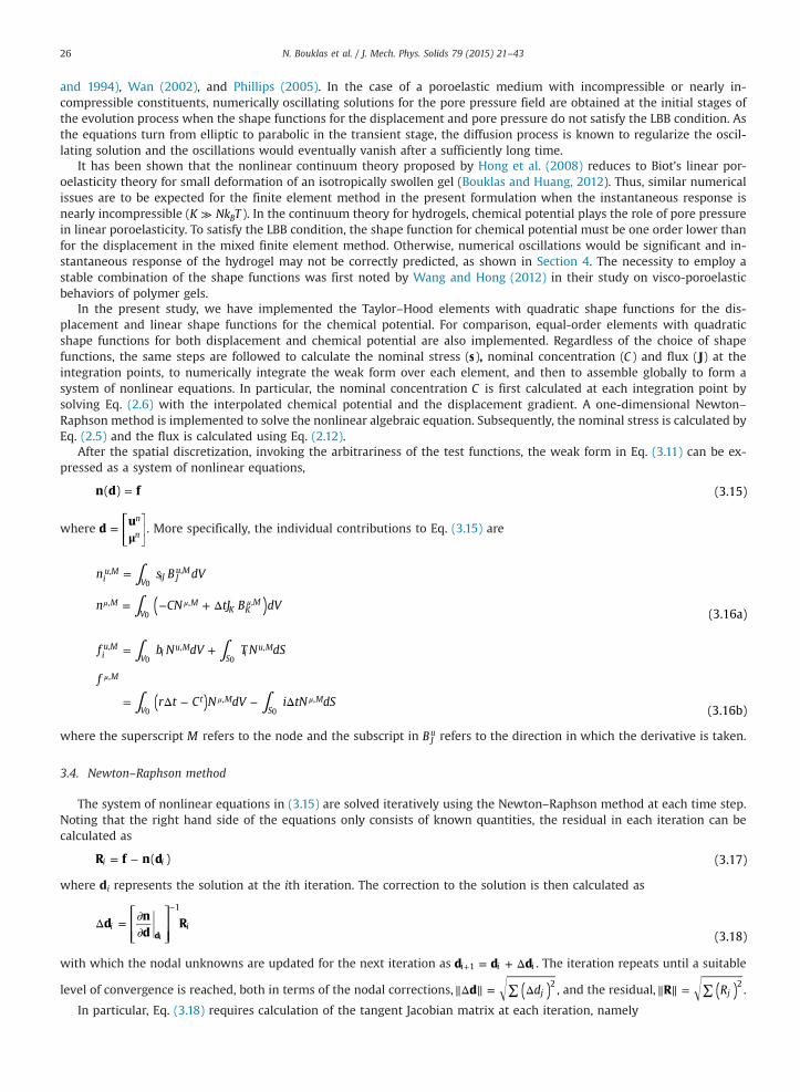
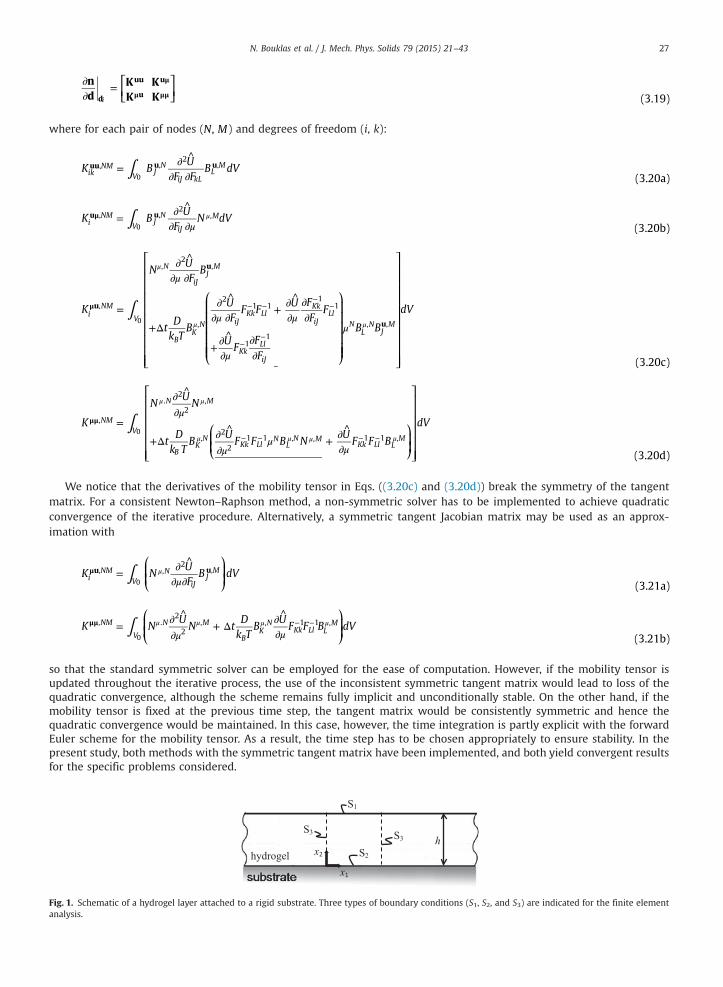
To illustrate the issue of numerical stability, we compare the results from two types of spatial interpolation (Fig. 2). First,using eight-node quadrilateral elements with equal-order biquadratic interpolation for both the displacement and chemicalpotential (8u8p), the numerical results show significant oscillations at the early stage (Fig. 3), which decay over time andeventually vanish. This is expected because the 8u8p elements with equal order interpolation violate the LBB condition.Here, a relatively large bulk modulus is used, K Nk T10 B

3= , to simulate a hydrogel with nearly incompressible constituents.The simulation domain is a square in the reference and initial states (a/H¼1) and is discretized by a uniform mesh with thenumber of elements along each side n 20e = . A 3 3× Gauss integration scheme is employed for full integration. The timestep is small at the early stage with t/ 10 5τΔ = − and it is gradually increased until the hydrogel reaches equilibrium.

It is found that the decay of the numerical oscillation depends on the element size. The maximum oscillation occurs inthe first layer of the elements below the surface, with an averaged amplitude, A ( 2 )/4max μ μ= ″ − ′ , where μ′ and μ″ are the

Fig. 2. Two types of quadrilateral elements: an equal-order eight-node element (8u8p) and a Taylor–Hood element (8u4p).

Fig. 3. Numerical oscillations of the chemical potential in the early stage of constrained swelling for a hydrogel layer with N 10 3Ω = − , 0.4χ = , K Nk T10 B3= ,and 1.40λ = , using the 8u8p elements with ne¼20.

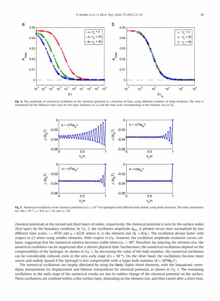
Fig. 4. The amplitude of numerical oscillation in the chemical potential as a function of time, using different numbers of 8u8p elements. The time isnormalized by the diffusion time scale for the layer thickness in (a) and the time scale corresponding to the element size in (b).

Fig. 5. Numerical oscillations of the chemical potential at t/ 10 4τ = − for hydrogels with different bulk moduli, using 8u8p elements. The other parametersare: N 10 3Ω = − , 0.4χ = , 1.40λ = , and ne¼20.


chemical potentials at the second and third layers of nodes, respectively; the chemical potential is zero for the surface nodes(first layer) by the boundary condition. In Fig. 4, the oscillation amplitude Amax is plotted versus time normalized by twodifferent time scales, H D/2τ = and h D/e e

2τ = , where he is the element size (h H n/e e= ). The oscillation decays faster withrespect to t/τ when using smaller elements. With respect to t/ eτ , however, the oscillation amplitude evolution curves col-lapse, suggesting that the numerical solution becomes stable when t/ 10e

4τ > . Therefore, by reducing the element size, thenumerical oscillation can be suppressed after a shorter physical time. Furthermore, the numerical oscillations depend on thecompressibility of the hydrogel. As shown in Fig. 5, by decreasing the value of the bulk modulus, the numerical oscillationcan be considerably reduced, even in the very early stage (t/ 10 4τ = − ). On the other hand, the oscillations become moresevere and widely spread if the hydrogel is less compressible with a larger bulk modulus (K Nk T10 B

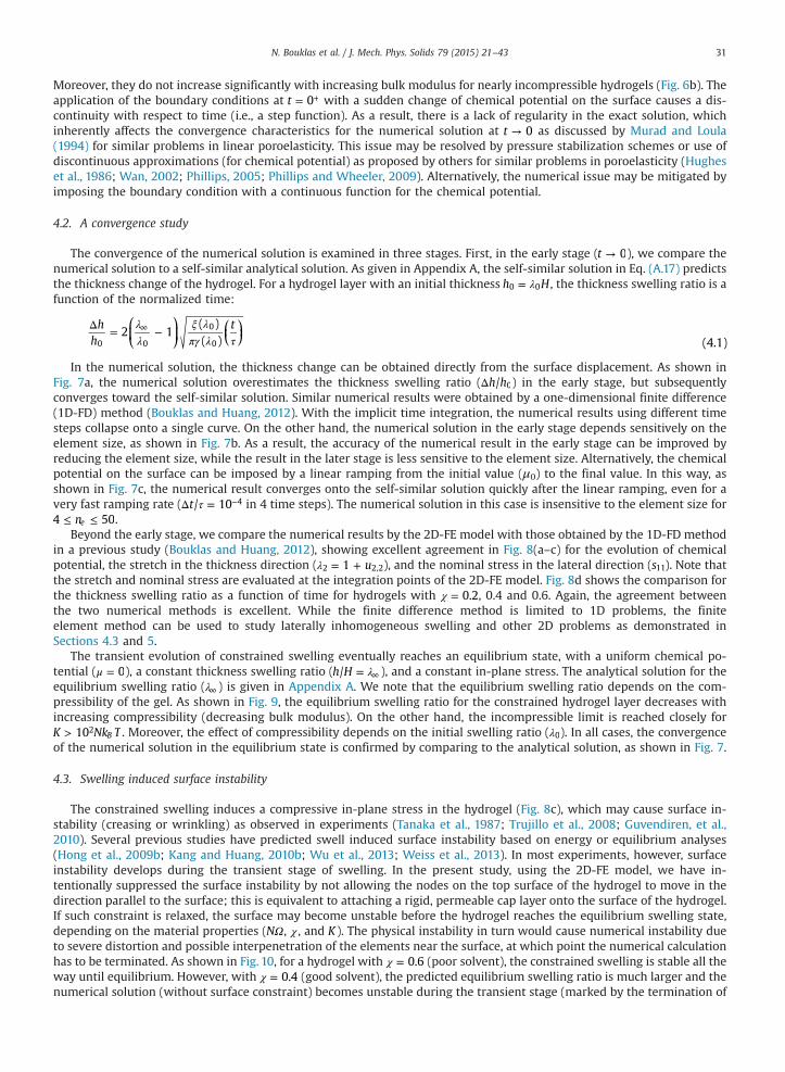
4= ).The numerical oscillations are largely alleviated by using the 8u4p Taylor–Hood elements, with the biquadratic seren-

dipity interpolation for displacement and bilinear interpolation for chemical potential, as shown in Fig. 6. The remainingoscillations in the early stage of the numerical results are due to sudden change of the chemical potential on the surface.These oscillations are confined within a thin surface layer, depending on the element size, and they vanish after a short time.

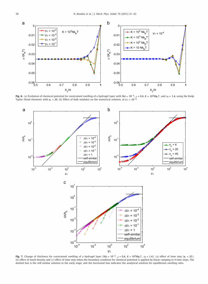
Fig. 6. (a) Evolution of chemical potential for constrained swelling of a hydrogel layer with N 10 3Ω = − , 0.4χ = , K Nk T10 B3= , and 1.40λ = , using the 8u4pTaylor–Hood elements with n 20e = . (b) Effect of bulk modulus on the numerical solution, at t/ 10 4τ = − .

Fig. 7. Change of thickness for constrained swelling of a hydrogel layer (N 10 3Ω = − , 0.4χ = , K Nk T10 B3= , 1.40λ = ): (a) effect of time step (n 20e = );(b) effect of mesh density and (c) effect of time step when the boundary condition for chemical potential is applied by linear ramping in 4 time steps. Thedashed line is the self-similar solution in the early stage, and the horizontal line indicates the analytical solution for equilibrium swelling ratio.



Moreover, they do not increase significantly with increasing bulk modulus for nearly incompressible hydrogels (Fig. 6b). Theapplication of the boundary conditions at t 0= + with a sudden change of chemical potential on the surface causes a dis-continuity with respect to time (i.e., a step function). As a result, there is a lack of regularity in the exact solution, whichinherently affects the convergence characteristics for the numerical solution at t 0→ as discussed by Murad and Loula(1994) for similar problems in linear poroelasticity. This issue may be resolved by pressure stabilization schemes or use ofdiscontinuous approximations (for chemical potential) as proposed by others for similar problems in poroelasticity (Hugheset al., 1986; Wan, 2002; Phillips, 2005; Phillips and Wheeler, 2009). Alternatively, the numerical issue may be mitigated byimposing the boundary condition with a continuous function for the chemical potential.

4.2. A convergence study

The convergence of the numerical solution is examined in three stages. First, in the early stage (t 0→ ), we compare thenumerical solution to a self-similar analytical solution. As given in Appendix A, the self-similar solution in Eq. (A.17) predictsthe thickness change of the hydrogel. For a hydrogel layer with an initial thickness h H0 0λ= , the thickness swelling ratio is afunction of the normalized time:

⎜ ⎟⎛⎝⎜

⎞⎠⎟

⎛⎝

⎞⎠

hh

t2 1

( )( ) (4.1)0 0

0

0

λλ

ξ λπγ λ τ

Δ = −∞

In the numerical solution, the thickness change can be obtained directly from the surface displacement. As shown inFig. 7a, the numerical solution overestimates the thickness swelling ratio ( h h/ 0Δ ) in the early stage, but subsequentlyconverges toward the self-similar solution. Similar numerical results were obtained by a one-dimensional finite difference(1D-FD) method (Bouklas and Huang, 2012). With the implicit time integration, the numerical results using different timesteps collapse onto a single curve. On the other hand, the numerical solution in the early stage depends sensitively on theelement size, as shown in Fig. 7b. As a result, the accuracy of the numerical result in the early stage can be improved byreducing the element size, while the result in the later stage is less sensitive to the element size. Alternatively, the chemicalpotential on the surface can be imposed by a linear ramping from the initial value (μ0) to the final value. In this way, asshown in Fig. 7c, the numerical result converges onto the self-similar solution quickly after the linear ramping, even for avery fast ramping rate ( t/ 10 4τΔ = − in 4 time steps). The numerical solution in this case is insensitive to the element size for

n4 50e≤ ≤ .Beyond the early stage, we compare the numerical results by the 2D-FE model with those obtained by the 1D-FD method

in a previous study (Bouklas and Huang, 2012), showing excellent agreement in Fig. 8(a–c) for the evolution of chemicalpotential, the stretch in the thickness direction ( u12 2,2λ = + ), and the nominal stress in the lateral direction (s11). Note thatthe stretch and nominal stress are evaluated at the integration points of the 2D-FE model. Fig. 8d shows the comparison forthe thickness swelling ratio as a function of time for hydrogels with 0.2χ = , 0.4 and 0.6. Again, the agreement betweenthe two numerical methods is excellent. While the finite difference method is limited to 1D problems, the finiteelement method can be used to study laterally inhomogeneous swelling and other 2D problems as demonstrated inSections 4.3 and 5.

The transient evolution of constrained swelling eventually reaches an equilibrium state, with a uniform chemical po-tential ( 0μ = ), a constant thickness swelling ratio (h H/ λ= ∞ ), and a constant in-plane stress. The analytical solution for theequilibrium swelling ratio (λ∞ ) is given in Appendix A. We note that the equilibrium swelling ratio depends on the com-pressibility of the gel. As shown in Fig. 9, the equilibrium swelling ratio for the constrained hydrogel layer decreases withincreasing compressibility (decreasing bulk modulus). On the other hand, the incompressible limit is reached closely forK Nk T10 B

2> . Moreover, the effect of compressibility depends on the initial swelling ratio ( 0λ ). In all cases, the convergenceof the numerical solution in the equilibrium state is confirmed by comparing to the analytical solution, as shown in Fig. 7.

4.3. Swelling induced surface instability

The constrained swelling induces a compressive in-plane stress in the hydrogel (Fig. 8c), which may cause surface in-stability (creasing or wrinkling) as observed in experiments (Tanaka et al., 1987; Trujillo et al., 2008; Guvendiren, et al.,2010). Several previous studies have predicted swell induced surface instability based on energy or equilibrium analyses(Hong et al., 2009b; Kang and Huang, 2010b; Wu et al., 2013; Weiss et al., 2013). In most experiments, however, surfaceinstability develops during the transient stage of swelling. In the present study, using the 2D-FE model, we have in-tentionally suppressed the surface instability by not allowing the nodes on the top surface of the hydrogel to move in thedirection parallel to the surface; this is equivalent to attaching a rigid, permeable cap layer onto the surface of the hydrogel.If such constraint is relaxed, the surface may become unstable before the hydrogel reaches the equilibrium swelling state,depending on the material properties (NΩ, χ , and K ). The physical instability in turn would cause numerical instability dueto severe distortion and possible interpenetration of the elements near the surface, at which point the numerical calculationhas to be terminated. As shown in Fig. 10, for a hydrogel with 0.6χ = (poor solvent), the constrained swelling is stable all theway until equilibrium. However, with 0.4χ = (good solvent), the predicted equilibrium swelling ratio is much larger and thenumerical solution (without surface constraint) becomes unstable during the transient stage (marked by the termination of

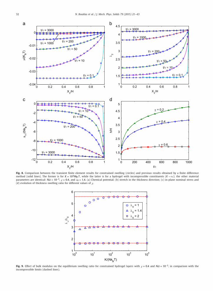
Fig. 9. Effect of bulk modulus on the equilibrium swelling ratio for constrained hydrogel layers with 0.4χ = and N 10 3Ω = − , in comparison with theincompressible limits (dashed lines).

Fig. 8. Comparison between the transient finite element results for constrained swelling (circles) and previous results obtained by a finite differencemethod (solid lines). The former is for K Nk T10 B3= , while the latter is for a hydrogel with incompressible constituents (K-1); the other materialparameters are identical: N 10 3Ω = − , 0.4χ = , and 1.40λ = . (a) Chemical potential; (b) stretch in the thickness direction; (c) in-plane nominal stress and(d) evolution of thickness swelling ratio for different values of χ .


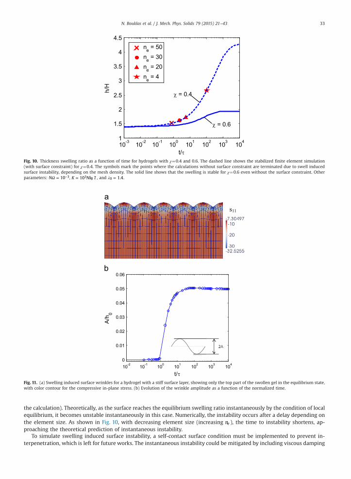
Fig. 10. Thickness swelling ratio as a function of time for hydrogels with χ¼0.4 and 0.6. The dashed line shows the stabilized finite element simulation(with surface constraint) for χ¼0.4. The symbols mark the points where the calculations without surface constraint are terminated due to swell inducedsurface instability, depending on the mesh density. The solid line shows that the swelling is stable for χ¼0.6 even without the surface constraint. Otherparameters: N 10 3Ω = − , K Nk T10 B3= , and 1.40λ = .

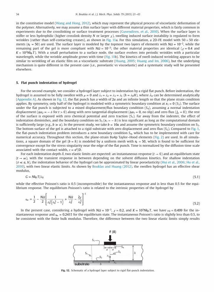
Fig. 11. (a) Swelling induced surface wrinkles for a hydrogel with a stiff surface layer, showing only the top part of the swollen gel in the equilibrium state,with color contour for the compressive in-plane stress. (b) Evolution of the wrinkle amplitude as a function of the normalized time.


the calculation). Theoretically, as the surface reaches the equilibrium swelling ratio instantaneously by the condition of localequilibrium, it becomes unstable instantaneously in this case. Numerically, the instability occurs after a delay depending onthe element size. As shown in Fig. 10, with decreasing element size (increasing ne ), the time to instability shortens, ap-proaching the theoretical prediction of instantaneous instability.

To simulate swelling induced surface instability, a self-contact surface condition must be implemented to prevent in-terpenetration, which is left for future works. The instantaneous instability could be mitigated by including viscous damping


in the constitutive model (Wang and Hong, 2012), which may represent the physical process of viscoelastic deformation ofthe polymer. Alternatively, we may assume a thin surface layer with different material properties, which is fairly common inexperiments due to the crosslinking or surface treatment processes (Guvendiren, et al., 2010). When the surface layer isstiffer or less hydrophilic (higher crosslink density N or larger χ), swelling induced surface instability is regulated to formwrinkles (rather than self-contacting creases), as shown in Fig. 11a. For this simulation, a 2D-FE model with 50�50 ele-ments (n 50e = ) are used. The surface layer is modeled by the topmost two layers of elements with N 10 2Ω = − , while theremaining part of the gel is more compliant with N 10 3Ω = − ; the other material properties are identical ( 0.4χ = andK Nk T10 B

3= ). With a small perturbation to a surface node, the surface evolves into periodic wrinkles with a particularwavelength, while the wrinkle amplitude grows with time (Fig. 11b). The kinetics of swell-induced wrinkling appears to besimilar to wrinkling of an elastic film on a viscoelastic substrate (Huang, 2005; Huang and Im, 2006), but the underlyingmechanism is quite different in the present case (i.e., poroelastic vs viscoelastic) and a systematic study will be presentedelsewhere.

5. Flat punch indentation of hydrogel

For the second example, we consider a hydrogel layer subject to indentation by a rigid flat punch. Before indentation, thehydrogel is assumed to be fully swollen with 0μ = and 1 2 3 0λ λ λ λ= = = (h H0λ= ), where λ0 can be determined analytically(Appendix A). As shown in Fig. 12, the flat punch has a width of a2 and an infinite length so that the plane strain conditionapplies. By symmetry, only half of the hydrogel is modeled with a symmetric boundary condition at x 01 = (S3). The surfaceunder the flat punch is subjected to a mixed displacement/flux boundary condition (S4), assuming a normal indentationdisplacement ( u2 δΔ = − for t 0> ) along with zero tangential displacement ( u 01Δ = , no slip) and zero flux ( J 02 = ); the restof the surface is exposed with zero chemical potential and zero traction (S1). Far away from the indenter, the effect ofindentation diminishes, and the boundary condition on S5 (x b1 = − ) is less significant as long as the computational domainis sufficiently large (e.g., b a≫ ). In the present study, we take b a10= and assume the symmetric boundary condition on S5.The bottom surface of the gel is attached to a rigid substrate with zero displacement and zero flux (S2). Compared to Fig. 1,the flat-punch indentation problem introduces a new boundary condition S4, which has to be implemented with care fornumerical accuracy. Throughout this section, the plane-strain 8u4p Taylor–Hood elements (Fig. 2) are used. In all simula-tions, a square domain of the gel (b h= ) is modeled by a uniform mesh with n 50e = , which is found to be sufficient forconvergence except for the stress singularity near the edge of the flat punch. Time is normalized by the diffusion time scaleassociated with the contact width, a D/2τ = .

For each indentation depth δ, two elastic limits are expected: an instantaneous response (t 0→ ) and an equilibrium state(t → ∞), with the transient response in between depending on the solvent diffusion kinetics. For shallow indentation( a h,δ ≪ ), the indentation behavior of the hydrogel can be approximated by linear poroelasticity (Hui et al., 2006; Hu et al.,2010), with two linear elastic limits. As shown by Bouklas and Huang (2012), the swollen hydrogel has an effective shearmodulus,

G Nk T/ (5.1)B 0λ=

while the effective Poisson’s ratio is 0.5 (incompressible) for the instantaneous response and is less than 0.5 for the equi-librium response. The equilibrium Poisson’s ratio is related to the intrinsic properties of the hydrogel by

⎡

⎣⎢⎢

⎤

⎦⎥⎥( )

N N12 2

1

1

2

(5.2)02

03

02

05

1

ν Ωλ λ

Ωλ

χλ

= −−

+ −∞

−

In the present case, considering a hydrogel with N 10 3Ω = − , 0.2χ = , and K Nk T10 B3= , we have 0.4990ν = for the in-

stantaneous response and 0.2415ν =∞ for the equilibrium state. The instantaneous Poisson’s ratio is slightly less than 0.5, tobe consistent with the finite bulk modulus. Therefore, the difference between the two linear elastic limits simply results

Fig. 12. Schematic of a hydrogel layer subject to rigid flat-punch indentation.

Fig. 13. Normalized indentation force versus depth at the two elastic limits, predicted by linear and nonlinear finite element methods, for a hydrogel with0.2χ = , N 10 3Ω = − and K Nk T10 B3= . The indenter half-width is a h/ 0.1= . The approximate analytical solution in Eq. (B.5) is shown as dashed lines for

comparison.


from the Poisson’s ratio effect. Using a linear elastic finite element model (LE-FEM) in ABAQUS Standard (ABAQUS, 2013)with the effective elastic properties of the hydrogel, we obtain the linear elastic limits for flat-punch indentation. Fig. 13plots the normalized indentation force versus the indentation depth at the elastic limits. The nearly incompressible in-stantaneous response imposes a numerical challenge even for the linear elastic model, which converges only for shallowindentation ( h/ 0.05δ < ). The numerical results are extrapolated linearly to deeper indentation for comparison. In addition,we present an approximate analytical solution in Appendix B based on an elastic half-space solution. However, as shown inFig. 13, the analytical solution considerably underestimates the indentation forces at the elastic limits for the hydrogel layersubject to a prescribed indentation depth. The presence of a rigid substrate underneath the hydrogel significantly increasesthe contact stiffness at both elastic limits under the plane strain condition, even for a very shallow indentation.

To simulate displacement controlled indentation of the hydrogel layer, the nodal displacements under the indenter arespecified as a function of time (e.g., a step function). Due to the intimate coupling between the solvent diffusion and thenetwork deformation, we have found that the application of the displacement boundary condition must be implementedwith some care. Specifically, the process of updating only the known displacement increments, followed by computing thetangent stiffness matrix and internal forces associated with this new artificial state, and then solving for the remainingdegrees of freedom leads to non-physical results. In particular, the instantaneous elastic limit is not correctly predicted usingthe above procedure. To obtain accurate numerical results for the flat-punch indentation at the instantaneous limit (t 0→ ), apenalty method (Hughes, 1987) was used in this work for the application of the displacement boundary condition under the

Fig. 14. (a) Indentation force as a function of time for a shallow indentation ( h/ 10 3δ = − ), in comparison with the linear elastic limits (dashed lines) forinstantaneous and equilibrium responses. (b) Normalized indentation force relaxation for various indentation depths, fitted by a function,

( )g t t t( / ) 0.25 exp( 7 / ) 0.75 exp /τ τ τ= − + − . Material parameters of the hydrogel are: 0.2χ = , N 10 3Ω = − , and K Nk T10 B3= .


indenter (S4). Essentially, as an approximation to the Lagrange multiplier method for imposing the displacement constraint,the tangent stiffness and residual in Eq. (3.18) are modified with sufficiently large spring stiffness associated with eachprescribed boundary displacement. We note that other methods utilizing the tangent stiffness based upon the prior de-formation and chemical potential state, and then applying the displacement boundary conditions can be implementedsuccessfully as well.

Fig. 14a shows the transient indentation relaxation behavior for a shallow indentation, h/ 10 3δ = − , bounded by the twolinear elastic limits (dashed lines). Similar results are obtained for relatively deep indentation up to h/ 0.2δ = . As shown inFig. 13, the instantaneous and equilibrium indentation forces obtained from the nonlinear finite element method (NL-FEM)are in good agreement with the linear elastic model in the shallow indentation regime ( h/ 0.05δ < ). As the indentation depthincreases, the linear elastic model (LE-FEM) becomes less accurate and underestimates the indentation forces at both limits.Following Hu et al. (2010), we re-normalize the force as F t F t F F F( ) ( ( ) ( ))/( (0) ( ))¯ = − ∞ − ∞ in Fig. 14b, where F (0) and F ( )∞are the two elastic limits obtained from the nonlinear finite element method. It is found that, for a specific set of material

Fig. 15. Evolution of the von Misses stress (left) and chemical potential (right) fields in a hydrogel layer ( 0.2χ = , N 10 3Ω = − , K Nk T10 B3= ) subject to flatpunch indentation with a h/ 0.1= and h/ 0.1δ = , at normalized time t/ 1, 10 , 10 , 102 4 7τ = (from top to bottom).

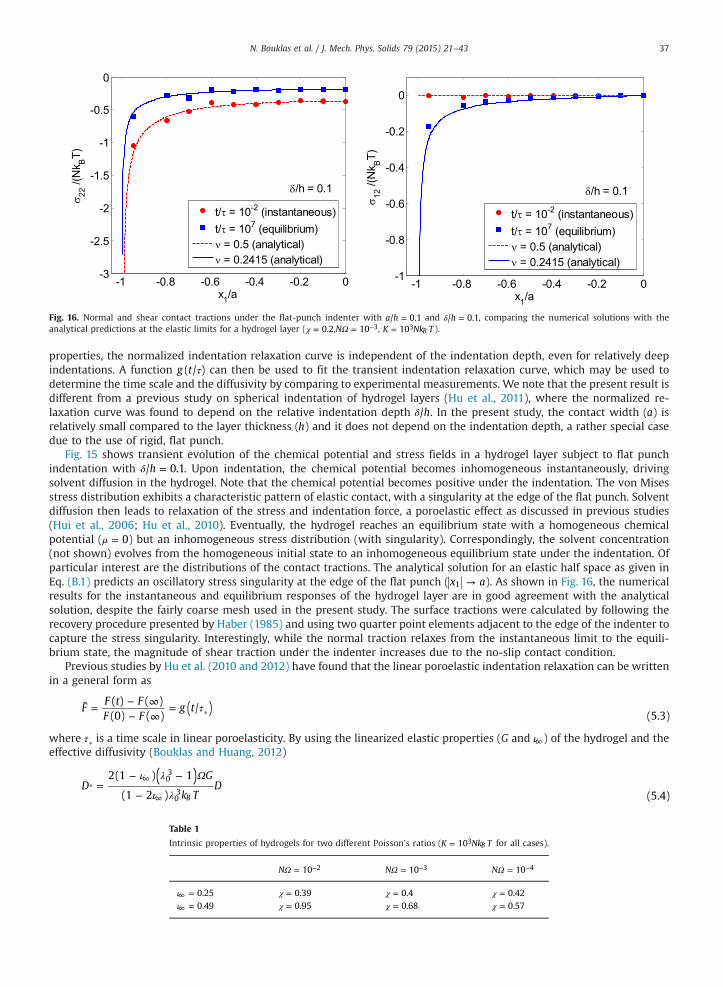
Fig. 16. Normal and shear contact tractions under the flat-punch indenter with a h/ 0.1= and h/ 0.1δ = , comparing the numerical solutions with theanalytical predictions at the elastic limits for a hydrogel layer ( 0.2χ = ,N 10 3Ω = − , K Nk T10 B3= ).


properties, the normalized indentation relaxation curve is independent of the indentation depth, even for relatively deepindentations. A function g t( / )τ can then be used to fit the transient indentation relaxation curve, which may be used todetermine the time scale and the diffusivity by comparing to experimental measurements. We note that the present result isdifferent from a previous study on spherical indentation of hydrogel layers (Hu et al., 2011), where the normalized re-laxation curve was found to depend on the relative indentation depth h/δ . In the present study, the contact width (a) isrelatively small compared to the layer thickness (h) and it does not depend on the indentation depth, a rather special casedue to the use of rigid, flat punch.

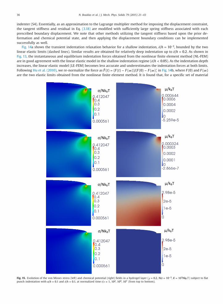
Fig. 15 shows transient evolution of the chemical potential and stress fields in a hydrogel layer subject to flat punchindentation with h/ 0.1δ = . Upon indentation, the chemical potential becomes inhomogeneous instantaneously, drivingsolvent diffusion in the hydrogel. Note that the chemical potential becomes positive under the indentation. The von Misesstress distribution exhibits a characteristic pattern of elastic contact, with a singularity at the edge of the flat punch. Solventdiffusion then leads to relaxation of the stress and indentation force, a poroelastic effect as discussed in previous studies(Hui et al., 2006; Hu et al., 2010). Eventually, the hydrogel reaches an equilibrium state with a homogeneous chemicalpotential ( 0μ = ) but an inhomogeneous stress distribution (with singularity). Correspondingly, the solvent concentration(not shown) evolves from the homogeneous initial state to an inhomogeneous equilibrium state under the indentation. Ofparticular interest are the distributions of the contact tractions. The analytical solution for an elastic half space as given inEq. (B.1) predicts an oscillatory stress singularity at the edge of the flat punch ( x a1 → ). As shown in Fig. 16, the numericalresults for the instantaneous and equilibrium responses of the hydrogel layer are in good agreement with the analyticalsolution, despite the fairly coarse mesh used in the present study. The surface tractions were calculated by following therecovery procedure presented by Haber (1985) and using two quarter point elements adjacent to the edge of the indenter tocapture the stress singularity. Interestingly, while the normal traction relaxes from the instantaneous limit to the equili-brium state, the magnitude of shear traction under the indenter increases due to the no-slip contact condition.

Previous studies by Hu et al. (2010 and 2012) have found that the linear poroelastic indentation relaxation can be writtenin a general form as

( )FF t FF F

g t( ) ( )(0) ( )

/(5.3)

τ¯ = − ∞− ∞

= ⁎

where τ⁎ is a time scale in linear poroelasticity. By using the linearized elastic properties (G and ν∞ ) of the hydrogel and theeffective diffusivity (Bouklas and Huang, 2012)

( )D

G

k TD

2(1 ) 1

(1 2 ) (5.4)B

03

03

ν λ Ω

ν λ=

− −

−⁎

∞

∞

Table 1

Intrinsic properties of hydrogels for two different Poisson’s ratios (K Nk T10 B3= for all cases).

N 10 2Ω = − N 10 3Ω = − N 10 4Ω = −

0.25ν =∞ 0.39χ = 0.4χ = 0.42χ =0.49ν =∞ 0.95χ = 0.68χ = 0.57χ =

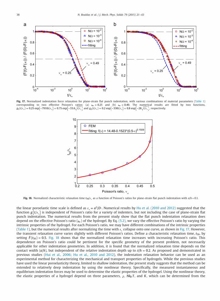
Fig. 17. Normalized indentation force relaxation for plane-strain flat punch indentation, with various combinations of material parameters (Table 1)corresponding to two effective Poisson’s ratios: (a) 0.25ν =∞ and (b) 0.49ν =∞ . The numerical results are fitted by two functions,

( )( )g t t t( / ) 0.25 exp 7910 / 0.75 exp 33.6 /1 τ τ τ= − + −⁎ ⁎ ⁎ and ( )( )g t t t( / ) 0.2 exp 330 / 0.8 exp 28 /2 τ τ τ= − + −⁎ ⁎ ⁎ , respectively.

Fig. 18. Normalized characteristic relaxation time t /50 τ⁎ as a function of Poisson’s ratios for plane-strain flat punch indentation with a/h¼0.1.


the linear poroelastic time scale is defined as a D/2τ =⁎⁎. Numerical results by Hu et al. (2010 and 2012) suggested that the

function ( )g t/τ⁎ is independent of Poisson’s ratio for a variety of indenters, but not including the case of plane-strain flatpunch indentation. The numerical results from the present study show that the flat punch indentation relaxation doesdepend on the effective Poisson’s ratio (ν∞ ) of the hydrogel. By Eq. (5.2), we vary the effective Poisson’s ratio by varying theintrinsic properties of the hydrogel. For each Poisson’s ratio, we may have different combinations of the intrinsic properties(Table 1), but the numerical results after normalizing the time with τ⁎ collapse onto one curve, as shown in Fig. 17. However,the transient relaxation curve varies slightly with different Poisson’s ratios. Define a characteristic relaxation time, t50, bysetting F t( ) 0.550¯ = . Fig. 18 shows that the normalized relaxation time increases with increasing Poisson’s ratio. Thisdependence on Poisson’s ratio could be pertinent for the specific geometry of the present problem, not necessarilyapplicable for other indentation geometries. In addition, it is found that the normalized relaxation time depends on thecontact width (a h/ ), but independent of the relative indentation depth up to h/ 0.2δ = . As proposed and demonstrated inprevious studies (Hui et al., 2006; Hu et al., 2010 and 2012), the indentation relaxation behavior can be used as anexperimental method for characterizing the mechanical and transport properties of hydrogels. While the previous studieshave used the linear poroelasticity theory, limited to shallow indentation, the present study suggests that the method can beextended to relatively deep indentation by using the nonlinear theory. Specifically, the measured instantaneous andequilibrium indentation forces may be used to determine the elastic properties of the hydrogel. Using the nonlinear theory,the elastic properties of a hydrogel depend on three parameters, χ , Nk TB , and K , which can be determined from the

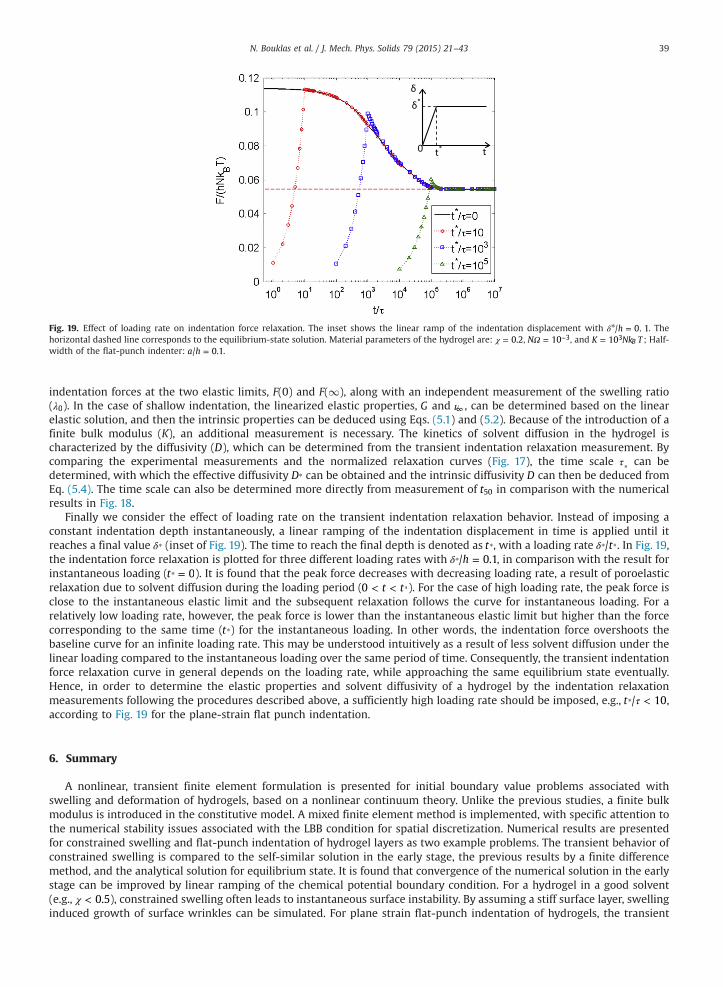
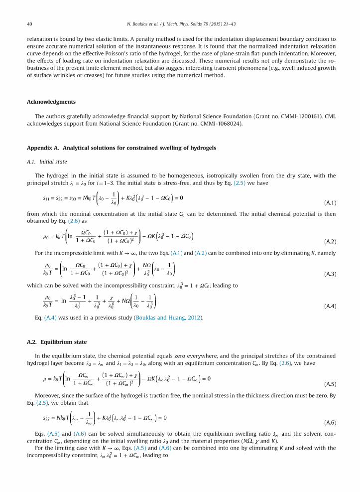
Fig. 19. Effect of loading rate on indentation force relaxation. The inset shows the linear ramp of the indentation displacement with h/ 0. 1δ* = . Thehorizontal dashed line corresponds to the equilibrium-state solution. Material parameters of the hydrogel are: 0.2χ = , N 10 3Ω = − , and K Nk T10 B3= ; Half-width of the flat-punch indenter: a h/ 0.1= .


indentation forces at the two elastic limits, F(0) and F(1), along with an independent measurement of the swelling ratio( 0λ ). In the case of shallow indentation, the linearized elastic properties, G and ν∞ , can be determined based on the linearelastic solution, and then the intrinsic properties can be deduced using Eqs. (5.1) and (5.2). Because of the introduction of afinite bulk modulus (K), an additional measurement is necessary. The kinetics of solvent diffusion in the hydrogel ischaracterized by the diffusivity (D), which can be determined from the transient indentation relaxation measurement. Bycomparing the experimental measurements and the normalized relaxation curves (Fig. 17), the time scale τ⁎ can bedetermined, with which the effective diffusivity D⁎ can be obtained and the intrinsic diffusivity D can then be deduced fromEq. (5.4). The time scale can also be determined more directly from measurement of t50 in comparison with the numericalresults in Fig. 18.

Finally we consider the effect of loading rate on the transient indentation relaxation behavior. Instead of imposing aconstant indentation depth instantaneously, a linear ramping of the indentation displacement in time is applied until itreaches a final value δ⁎ (inset of Fig. 19). The time to reach the final depth is denoted as t⁎, with a loading rate t/δ⁎ ⁎. In Fig. 19,the indentation force relaxation is plotted for three different loading rates with h/ 0.1δ =⁎ , in comparison with the result forinstantaneous loading (t 0=⁎ ). It is found that the peak force decreases with decreasing loading rate, a result of poroelasticrelaxation due to solvent diffusion during the loading period ( t t0 < < ⁎). For the case of high loading rate, the peak force isclose to the instantaneous elastic limit and the subsequent relaxation follows the curve for instantaneous loading. For arelatively low loading rate, however, the peak force is lower than the instantaneous elastic limit but higher than the forcecorresponding to the same time (t⁎) for the instantaneous loading. In other words, the indentation force overshoots thebaseline curve for an infinite loading rate. This may be understood intuitively as a result of less solvent diffusion under thelinear loading compared to the instantaneous loading over the same period of time. Consequently, the transient indentationforce relaxation curve in general depends on the loading rate, while approaching the same equilibrium state eventually.Hence, in order to determine the elastic properties and solvent diffusivity of a hydrogel by the indentation relaxationmeasurements following the procedures described above, a sufficiently high loading rate should be imposed, e.g., t / 10τ <⁎ ,according to Fig. 19 for the plane-strain flat punch indentation.

6. Summary

A nonlinear, transient finite element formulation is presented for initial boundary value problems associated withswelling and deformation of hydrogels, based on a nonlinear continuum theory. Unlike the previous studies, a finite bulkmodulus is introduced in the constitutive model. A mixed finite element method is implemented, with specific attention tothe numerical stability issues associated with the LBB condition for spatial discretization. Numerical results are presentedfor constrained swelling and flat-punch indentation of hydrogel layers as two example problems. The transient behavior ofconstrained swelling is compared to the self-similar solution in the early stage, the previous results by a finite differencemethod, and the analytical solution for equilibrium state. It is found that convergence of the numerical solution in the earlystage can be improved by linear ramping of the chemical potential boundary condition. For a hydrogel in a good solvent(e.g., 0.5χ < ), constrained swelling often leads to instantaneous surface instability. By assuming a stiff surface layer, swellinginduced growth of surface wrinkles can be simulated. For plane strain flat-punch indentation of hydrogels, the transient


relaxation is bound by two elastic limits. A penalty method is used for the indentation displacement boundary condition toensure accurate numerical solution of the instantaneous response. It is found that the normalized indentation relaxationcurve depends on the effective Poisson’s ratio of the hydrogel, for the case of plane strain flat-punch indentation. Moreover,the effects of loading rate on indentation relaxation are discussed. These numerical results not only demonstrate the ro-bustness of the present finite element method, but also suggest interesting transient phenomena (e.g., swell induced growthof surface wrinkles or creases) for future studies using the numerical method.

Acknowledgments

The authors gratefully acknowledge financial support by National Science Foundation (Grant no. CMMI-1200161). CMLacknowledges support from National Science Foundation (Grant no. CMMI-1068024).

Appendix A. Analytical solutions for constrained swelling of hydrogels

A.1. Initial state

The hydrogel in the initial state is assumed to be homogeneous, isotropically swollen from the dry state, with theprincipal stretch i 0λ λ= for i¼1–3. The initial state is stress-free, and thus by Eq. (2.5) we have

⎛⎝⎜

⎞⎠⎟ ( )s s s Nk T K C

11 0

(A.1)B11 22 33 0

002

03

0λλ

λ λ Ω= = = − + − − =

from which the nominal concentration at the initial state C0 can be determined. The initial chemical potential is thenobtained by Eq. (2.6) as

⎛⎝⎜⎜

⎞⎠⎟⎟ ( )k T

CC

C

CK Cln

1(1 )

(1 )1

(A.2)B0

0

0

0

02 0

30μ

ΩΩ

Ω χΩ

Ω λ Ω=+

++ +

+− − −

For the incompressible limit with K → ∞, the two Eqs. (A.1) and (A.2) can be combined into one by eliminating K, namely

⎛⎝⎜⎜

⎞⎠⎟⎟

⎛⎝⎜

⎞⎠⎟k T

CC

C

CN

ln1

(1 )

(1 )1

(A.3)B

0 0

0

0

02

02 0

0

μ ΩΩ

Ω χΩ

Ωλ

λλ

=+

++ +

++ −

which can be solved with the incompressibility constraint, C103

0λ Ω= + , leading to

⎛⎝⎜⎜

⎞⎠⎟⎟k T

Nln1 1 1 1

(A.4)B

0 03

03

03

06 0 0

3

μ λλ λ

χλ

Ωλ λ

=−

+ + + −

Eq. (A.4) was used in a previous study (Bouklas and Huang, 2012).

A.2. Equilibrium state

In the equilibrium state, the chemical potential equals zero everywhere, and the principal stretches of the constrainedhydrogel layer become 2λ λ= ∞ and 1 3 0λ λ λ= = , along with an equilibrium concentration C∞ . By Eq. (2.6), we have

⎛⎝⎜⎜

⎞⎠⎟⎟ ( )k T

CC

C

CK Cln

1(1 )

(1 )1 0

(A.5)B 2 0

2μΩ

ΩΩ χ

ΩΩ λ λ Ω=

++

+ ++

− − − =∞

∞

∞

∞∞ ∞

Moreover, since the surface of the hydrogel is traction free, the nominal stress in the thickness direction must be zero. ByEq. (2.5), we obtain that

⎛⎝⎜

⎞⎠⎟ ( )s Nk T K C

11 0

(A.6)B22 0

202λ

λλ λ λ Ω= − + − − =∞

∞∞ ∞

Eqs. (A.5) and (A.6) can be solved simultaneously to obtain the equilibrium swelling ratio λ∞ and the solvent con-centration C∞ , depending on the initial swelling ratio 0λ and the material properties (NΩ, χ and K).

For the limiting case with K → ∞, Eqs. (A.5) and (A.6) can be combined into one by eliminating K and solved with theincompressibility constraint, C10

2λ λ Ω= +∞ ∞ , leading to


⎛⎝⎜

⎞⎠⎟

Nln

1 1 10

(A.7)02

02

02 2

04

02

λ λλ λ λ λ

χλ λ

Ωλ

λλ

−+ + + − =∞

∞ ∞ ∞∞

∞

which was used in the previous study (Bouklas and Huang, 2012).

A.3. Early stage of swelling: a self-similar solution

The transient process of constrained swelling can be described by a nonlinear diffusion equation. With the principalstretch X t( , )2 2λ and the solvent concentration C(X2, t), the chemical potential by Eq. (2.6) is

⎛⎝⎜⎜

⎞⎠⎟⎟ ( )k T

CC

C

CK Cln

1(1 )

(1 )1

(A.8)B 2 2 0

2μ ΩΩ

Ω χΩ

Ω λ λ Ω=+

++ +

+− − −

The traction-free boundary condition on the surface requires that the nominal stress in the thickness direction be zero,namely

⎛⎝⎜

⎞⎠⎟ ( )s Nk T K C

11 0

(A.9)B22 2

202

2 02λ

λλ λ λ Ω= − + − − =

giving an expression for the nominal concentration as a function of the principal stretch

⎡⎣⎢

⎛⎝⎜

⎞⎠⎟

⎤⎦⎥C

Nk T

K1 1

1(A.10)

B

02 2

22 0

2

Ω λλ

λλ λ= − + −

The flux in the thickness direction is obtained from Eq. (2.12) as

J MX

DCk T X (A.11)B

2 222 2

22

μλ

μ= − ∂∂

= − ∂∂

Substituting (A.10) and (A.11) into Eq. (2.14) with r¼0 (assuming no source), we obtain that

⎡⎣⎢

⎤⎦⎥t

DX X

( ) ( )(A.12)

22

22

2

2γ λ

λξ λ

λ∂∂

= ∂∂

∂∂

where

⎛⎝⎜⎜

⎞⎠⎟⎟C Nk T

K( ) 1

1

(A.13)B

22

02

02

22

γ λ Ωλ

λλ λ

= ∂∂

= + +

⎛⎝⎜

⎞⎠⎟

⎛⎝⎜⎜

⎞⎠⎟⎟

⎛

⎝⎜⎜

⎞

⎠⎟⎟

( ) ( )Ck T C

CC

C

C

Nk T

K

N C( )

1(1 )

2(1 )

1 1

(A.14)B

B2

22

2 2 2 3

22

02

24

02

22

222

02

24

ξ λ Ωλ

μλ

μλ Ω

χΩΩ

λ

λ λλλ

Ω λ

λ λ= ∂

∂∂∂

+ ∂∂

=+

−+

++ +

+

At the early stage of swelling (t-0), the nonlinear diffusion equation (A.12) can be linearized as

tD

X

( )( ) (A.15)

2 0

0

22

22

λ ξ λγ λ

λ∂∂

=∂∂

leading to a self-similar solution

⎛⎝⎜⎜

⎞⎠⎟⎟erfc

H XD t

( )2

( )( ) (A.16)

2 0

0

2 0

0

λ λλ λ

γ λξ λ

−−

=−

∞

The change of the thickness of the hydrogel layer is then obtained as

h t dXDt

( ) ( ) 2( )( )( ) (A.17)

H2 0 2 0

0

0∫ λ λ λ λ

ξ λγ λ π

Δ = − = −−∞

∞

For the limiting case with K → ∞ and using the incompressibility constraint, C103λ Ω= + , it can be shown that the self-

similar solutions given by Eqs. (A.16) and (A.17) recover those in our previous study (Bouklas and Huang, 2012), with

( )0 02γ λ λ→ and N( )0

1 2 ( 1) ( 1)( 1)

06

03

09

03

02

06ξ λ Ω→ − +

λ

χ λ

λ

λ λ

λ

− − +. As noted in the previous study, a similar solution was obtained in

linear poroelasticity (Yoon et al., 2010; Doi, 2009).


Appendix B. An analytical solution for flat punch indentation of an elastic half space

Several textbooks have presented analytical solutions for plane-strain indentation of an elastic half space using a rigidflat punch (e.g., Johnson, 1985; Bower, 2010). Assuming no slip in the contact region of the surface, the normal and sheartractions on the contact surface (x a< ) can be written as

⎜ ⎟⎛⎝

⎞⎠i

F

a x

a xa x

2(1 )3 4 (B.1)

i

2 2σ τ ν

ν π+ = − −

− −

+−

η

where ν is Poisson’s ratio, ln(3 4 )12

η ν= −π

and F is the total normal force (per unit length). Note that the stress field has an

oscillatory singularity at the edge of the flat punch (x a→ ) unless 0.5ν = .To determine the indentation displacement, however, a point of datum has to be used. An analytical solution for the

general case is possible but too lengthy to be included here. As a special case for 0.5ν = , we have 0τ = and the solutioncoincides with that of frictionless contact with

F

a x (B.2)2 2σ

π= −

−

Following the complex variable method in Bower (2010), the displacement at a point located on the line of symmetry(x¼0) under the indenter can be obtained as

( )u yF

Gy y a d(0, )

(1 )ln (B.3)y

2 2νπ

= −−

+ + +

where y is the distance from the surface and G is shear modulus of the material. Taking the point at y¼h as a datum withzero displacement, we obtain that

( )dF

Gh h a

(1 )ln (B.4)

2 2νπ

=−

+ +

The surface displacement under the flat punch indenter is then

⎛

⎝⎜⎜

⎛⎝⎜

⎞⎠⎟

⎞

⎠⎟⎟u

FG

ha

ha

(0, 0)(1 )

ln 1(B.5)

y

2

δν

π= =

−+ +

As noted in Fig. 13, Eq. (B.5) considerably overestimates the indentation displacement for an elastic layer of thickness h.Apparently, the elastic layer has a much larger contact stiffness due to the presence of a rigid substrate, even for a veryshallow indentation under the plane strain condition.

References

ABAQUS, 2013. ABAQUS 6.13 User Documentation, by Dassault Systèmes Simulia Corp., Providence, RI.Babuška, I., 1971. Error-bounds for finite element method. Numer. Math. 16 (4), 322–333.Biot, M.A., 1941. General theory of three‐dimensional consolidation. J. Appl. Phys. 12 (2), 155–164.Birgersson, E., Li, H., Wu, S., 2008. Transient analysis of temperature-sensitive neutral hydrogels. J. Mech. Phys. Solids 56 (2), 444–466.Bouklas, N., Huang, R., 2012. Swelling kinetics of polymer gels: comparison of linear and nonlinear theories. Soft Matter 8 (31), 8194–8203.Borja, R.I., 1986. Finite element formulation for transient pore pressure dissipation: a variational approach. Int. J. Solids and Struct. 22 (11), 1201–1211.Bower, A.F., 2010. In: Applied Mechanics of SolidsCRC Press, Boca Raton, FL.Brezzi, F., 1974. On the existence, uniqueness and approximation of saddle-point problems arising from Lagrangian multipliers. ESAIM: Math. Model.

Numer. Anal.-Modél. Math. Anal. Numér. 8 (R2), 129–151.Chan, E.P., Hu, Y., Johnson, P.M., Suo, Z., Stafford, C.M., 2012. Spherical indentation testing of poroelastic relaxations in thin hydrogel layers. Soft Matter 8 (5),

1492–1498.Chester, S.A., Anand, L., 2010. A coupled theory of fluid permeation and large deformations for elastomeric materials. J. Mech. Phys. Solids 58 (11),

1879–1906.Doi, M., 2009. Gel dynamics. J. Phys. Soc. Jpn. 78 (5), 052001.Dolbow, J., Fried, E., Ji, H., 2004. Chemically induced swelling of hydrogels. J. Mech. Phys. Solids 52 (1), 51–84.Duda, F.P., Souza, A.C., Fried, E., 2010. A theory for species migration in a finitely strained solid with application to polymer network swelling. J. Mech. Phys.

Solids 58 (4), 515–529.Galli, M., Oyen, M.L., 2009. Fast identification of poroelastic parameters from indentation tests. Comput. Model. Eng. Sci. (CMES) 48 (3), 241–268.Guvendiren, M., Burdick, J.A., Yang, S., 2010. Kinetic study of swelling-induced surface pattern formation and ordering in hydrogel films with depth-wise

crosslinking gradient. Soft Matter 6 (9), 2044–2049.Haber, R.B., 1985. A consistent finite element technique for recovery of distributed reactions and surface tractions. Int. J. Numer. Methods Eng. 21 (11),

2013–2025.Hong, W., Liu, Z., Suo, Z., 2009a. Inhomogeneous swelling of a gel in equilibriumwith a solvent and mechanical load. Int. J. Solids Struct. 46 (17), 3282–3289.Hong, W., Zhao, X., Suo, Z., 2009b. Formation of creases on the surfaces of elastomers and gels. Appl. Phys. Lett. 95 (11), 111901.Hong, W., Zhao, X., Zhou, J., Suo, Z., 2008. A theory of coupled diffusion and large deformation in polymeric gels. J. Mech. Phys. Solids 56 (5), 1779–1793.Hu, Y., Zhao, X., Vlassak, J.J., Suo, Z., 2010. Using indentation to characterize the poroelasticity of gels. Appl. Phys. Lett. 96 (12), 121904.Hu, Y., Chan, E.P., Vlassak, J.J., Suo, Z., 2011. Poroelastic relaxation indentation of thin layers of gels. J. Appl. Phys. 110, 086103.

http://refhub.elsevier.com/S0022-5096(15)00060-5/sbref1










































Hu, Y., You, J.O., Auguste, D.T., Suo, Z., Vlassak, J.J., 2012. Indentation: a simple, nondestructive method for characterizing the mechanical and transportproperties of pH-sensitive hydrogels. J. Mater. Res. 27, 152–160.

Huang, R., 2005. Kinetic wrinkling of an elastic film on a viscoelastic substrate. J. Mech. Phys. Solids 53, 63–89.Huang, R., Im, S.H., 2006. Dynamics of wrinkle growth and coarsening in stressed thin films. Phys. Rev. E 74 (2), 026214.Hughes, T.J.R., 1987. The Finite Element Method: Linear Static and Dynamic Finite Element Analysis. Prentice Hall, Englewood Cliffs, NJ.Hughes, T.J.R., Franca, L.P., Balestra, M., 1986. A new finite element formulation for computational fluid dynamics: V. Circumventing the Babuška–Brezzi

condition: a stable Petrov–Galerkin formulation of the Stokes problem accommodating equal-order interpolations. Comput. Methods Appl. Mech. Eng.59 (1), 85–99.

Hui, C.Y., Lin, Y.Y., Chuang, F.C., Shull, K.R., Lin, W.C., 2006. A contact mechanics method for characterizing the elastic properties and permeability of gels. J.Polym. Sci. Part B: Polym. Phys. 44 (2), 359–370.

Johnson, K.L., 1985. In: Contact MechanicsCambridge University Press, Cambridge, UK.Kalcioglu, Z.I., Mahmoodian, R., Hu, Y., Suo, Z., Van Vliet, K.J., 2012. From macro-to microscale poroelastic characterization of polymeric hydrogels via

indentation. Soft Matter 8 (12), 3393–3398.Kang, M.K., Huang, R., 2010a. A variational approach and finite element implementation for swelling of polymeric hydrogels under geometric constraints. J.

Appl. Mech. 77 (6), 061004.Kang, M.K., Huang, R., 2010b. Swell-induced surface instability of confined hydrogel layers on substrates. J. Mech. Phys. Solids 58 (10), 1582–1598.Lucantonio, A., Nardinocchi, P., Teresi, L., 2013. Transient analysis of swelling-induced large deformations in polymer gels. J. Mech. Phys. Solids 61 (1),

205–218.Murad, M.A., Loula, A.F., 1992. Improved accuracy in finite element analysis of Biot’s consolidation problem. Comput. Methods Appl. Mech. Eng. 95 (3),

359–382.Murad, M.A., Loula, A.F., 1994. On stability and convergence of finite element approximations of Biot’s consolidation problem. Int. J. Numer. Methods Eng. 37

(4), 645–667.Phillips, P.J., 2005. Finite element methods in linear poroelasticity: theoretical and computational results. University of Texas at Austin Ph.D. dissertation.Phillips, P.J., Wheeler, M.F., 2009. Overcoming the problem of locking in linear elasticity and poroelasticity: an heuristic approach. Comput. Geosci. 13 (1),

5–12.Rice, J.R., Cleary, M.P., 1976. Some basic stress diffusion solutions for fluid‐saturated elastic porous media with compressible constituents. Rev. Geophys. 14

(2), 227–241.Scherer, G.W., 1989. Measuring of permeability I. Theory. J. Non-Cryst. Solids 113, 107–118.Sussman, T., Bathe, K.J., 1987. A finite element formulation for the nonlinear incompressible elastic and inelastic analysis. Comput. Struct. 26 (1), 357–409.Tanaka, T., Hocker, L., Benedek, G., 1973. Spectrum of light scattered from a viscoelastic gel. J. Chem. Phys. 59, 5151–5159.Tanaka, T., Sun, S.T., Hirokawa, Y., Katayama, S., Kucera, J., Hirose, Y., Amiya, T., 1987. Mechanical instability of gels at the phase transition. Nature 325,

796–798.Taylor, C., Hood, P., 1973. A numerical solution of the Navier–Stokes equations using the finite element technique. Comput. Fluids 1, 73–100.Trujillo, V., Kim, J., Hayward, R.C., 2008. Creasing instability of surface-attached hydrogels. Soft Matter 4, 564–569.Toh, W., Liu, Z., Ng, T.Y., Hong, W., 2013. Inhomogeneous large deformation kinetics of polymeric gels. Int. J. Appl. Mech. 5, 1350001.Vermeer, P.A., Verruijt, A., 1981. An accuracy condition for consolidation by finite elements. Int. J. Numer. Anal. Methods Geomech. 5, 1–14.Wan, J., 2002. Stabilized finite element methods for coupled geomechanics and multiphase flow. Stanford University Ph.D. dissertation.Wang, X., Hong, W., 2012. A visco-poroelastic theory for polymeric gels. Proc. R. Soc. A: Math. Phys. Eng. Sci. 468, 3824–3841.Weiss, F., Cai, S., Hu, Y., Kang, M.K., Huang, R., Suo, Z., 2013. Creases and wrinkles on the surface of a swollen gel. J. Appl. Phys. 114 (7), 073507.White, J.A., Borja, R.I., 2008. Stabilized low-order finite elements for coupled solid-deformation/fluid-diffusion and their application to fault zone transients.

Comput. Methods Appl. Mech. Eng. 197 (49), 4353–4366.Wu, Z., Bouklas, N., Huang, R., 2013. Swell-induced surface instability of hydrogel layers with material properties varying in thickness direction. Int. J. Solids

Struct. 50, 578–587.Yoon, J., Cai, S., Suo, Z., Hayward, R.C., 2010. Poroelastic swelling kinetics of thin hydrogel layers: comparison of theory and experiment. Soft Matter 6 (23),

6004–6012.Zhang, J., Zhao, X., Suo, Z., Jiang, H., 2009. A finite element method for transient analysis of concurrent large deformation and mass transport in gels. J. Appl.

Phys. 105 (9), 093522.Zienkiewicz, O.C., Chan, A.H.C., Pastor, M., Paul, D.K., Shiomi, T., 1990. Static and dynamic behavior of soils: a rational approach to quantitative solutions. I.

Fully saturated problems. Proc. R. Soc. Lond. A. Math. Phys. Sci. 429, 285–309.









































































a nonlinear, transient finite element method for coupled …ruihuang/papers/jmps07.pdf · ·...

Documents