transient analysis model of a nonlinear magnetic circuit
TRANSCRIPT
Transient analysis model of a nonlinear magnetic circuit for developing a computer-aided design tool of flux-gate current sensors
Eiji Hashiguchi a, Takafumi Koseki a, Eric Favre b, Masahiro Ashiya b, Toshifumi Tachibana b a Graduate School of Engineering, Koseki laboratory, 7-3-1 Hongo, Bunkyo-ku Tokyo, 113-8656, Japan
b Nana-LEM, 2-1-2 Nakamachi, Machida-shi Tokyo, 194-0021, Japan
Abstract — The authors have made a fundamental model of a flux-gate current sensor based on a magnetic circuit. The authors have tried two different numerical methods; the first one is the fourth Runge-Kutta method and the second one is the method by connecting analytic solutions. Although both numerical schemes have been derived from identical differential equations, only the results of the latter method are plausible. The authors propose the latter method as a reliable calculation tool for actual designs of flux-gate current sensors from the comparison of their numerical and experimental results.
Keywords — Flux-gate, nonlinear, magnetic circuit, saturation, hysteresis
I. MAGNETIC CIRCUIT MODELING
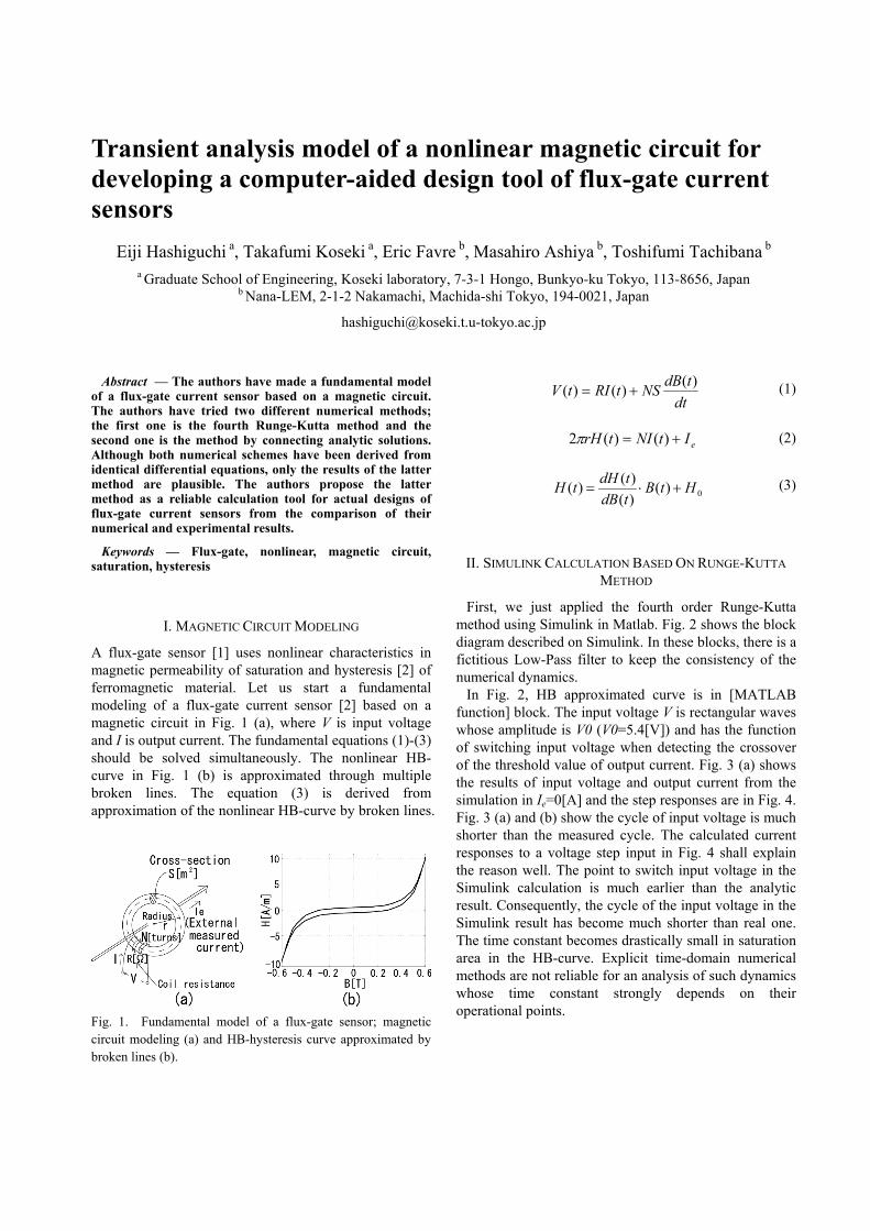
A flux-gate sensor [1] uses nonlinear characteristics in magnetic permeability of saturation and hysteresis [2] of ferromagnetic material. Let us start a fundamental modeling of a flux-gate current sensor [2] based on a magnetic circuit in Fig. 1 (a), where V is input voltage and I is output current. The fundamental equations (1)-(3) should be solved simultaneously. The nonlinear HB-curve in Fig. 1 (b) is approximated through multiple broken lines. The equation (3) is derived from approximation of the nonlinear HB-curve by broken lines. Fig. 1. Fundamental model of a flux-gate sensor; magnetic circuit modeling (a) and HB-hysteresis curve approximated by broken lines (b).
dttdBNStRItV )()()( += (1)
eItNItrH += )()(2π (2)
0)(
)()()( HtB
tdBtdHtH +⋅= (3)
II. SIMULINK CALCULATION BASED ON RUNGE-KUTTA METHOD
First, we just applied the fourth order Runge-Kutta method using Simulink in Matlab. Fig. 2 shows the block diagram described on Simulink. In these blocks, there is a fictitious Low-Pass filter to keep the consistency of the numerical dynamics.
In Fig. 2, HB approximated curve is in [MATLAB function] block. The input voltage V is rectangular waves whose amplitude is V0 (V0=5.4[V]) and has the function of switching input voltage when detecting the crossover of the threshold value of output current. Fig. 3 (a) shows the results of input voltage and output current from the simulation in Ie=0[A] and the step responses are in Fig. 4. Fig. 3 (a) and (b) show the cycle of input voltage is much shorter than the measured cycle. The calculated current responses to a voltage step input in Fig. 4 shall explain the reason well. The point to switch input voltage in the Simulink calculation is much earlier than the analytic result. Consequently, the cycle of the input voltage in the Simulink result has become much shorter than real one. The time constant becomes drastically small in saturation area in the HB-curve. Explicit time-domain numerical methods are not reliable for an analysis of such dynamics whose time constant strongly depends on their operational points.

III. THE ANALYSIS BY CONNECTING APPROXIMATE LOCAL ANALYTIC SOLUTIONS
Second, we solved the differential equation by connecting local analytic solutions. From fundamental equations (1)-(3) described above, the following state equation (4) and output equation (5) are derived.
−++
⋅
−=
)(2)(1
)()(2)(
0
2
tHNrRI
NRtV
NS
tBtdBdH
SNrR
dttdB
eπ
π
(4)
))(2(1)( eItrHN
tI −= π (5)
We led the successive form connecting local analytic
solution based on the transition matrix from equation (4) and (5). The equation (6) is a digital state equation and the equation (7) is the output equation, where Ts is time step and A(n) and u(n) are as following equations (8) and (9) whose symbols were defined in Fig. 1.
)()(
1)()1()(
)( nunA
enBenBs
s
TnATnA −
+⋅=+ (6)
))(2(1)( eInrHN
nI −= π (7)
)()(2)( 2 ndBdH
SNnrHnA π
−= (8)
−+= )(2)(1)( 0 nH
NrRI
NRnV
NSnu e
π (9)
Fig. 3. Input voltage and output current (Ie=0[A]); Simulink (a), measurement (b), and analytic solution (c).
Fig.2 Block diagram described on Simulink.
Fig.4 Step responses of coil current

The results of the simulations are similar to the measurement in Fig. 3 (b) and (c). Fig. 5 (a) and (b) show the results of the simulation when Ie ≠ 0. Output current flows through a resistance (5.1[kΩ ]) and RC-integrating circuit whose cut off frequency fc=0.05[Hz], and then measure the output value in an actual measurement. We have also used the transition matrix method in the simulation of RC integrating circuit. This result is shown in Fig. 6. We can conclude that the second simulator based on the connection of the local analytic solutions gives plausible calculation.
Fig. 5. Simulation results by analytic solution; input voltage and output current in Ie=1[A] (a) and Ie=-1[A] (b).
Fig. 6. Relation the final integrated output voltage and the external current Ie.
IV. THE EFFECTS OF HYSTERESIS IN MAGNETIZATION CHARACTERISTIC
We made this simulation by changing hysteresis characteristics in the magnetic core in order to evaluate the effects of hysteresis to output voltage. The used approximated magnetic curves are shown in Fig. 7 (a) and these simulation results are shown in Fig. 7 (b).
All the curves in Fig. 7 (b) are linear although the very exaggerated hysteresis slightly affected the gradient of the line. This means the substantial magnetic nonlinearity for the current sensing principle of this type of sensors is saturation and hysteresis plays minor roles in the measurement. That is to say, it is important for designers to select a core material of strong saturation and of small hysteresis in order to reduce its excitation loss.
Fig. 7. Simulation results in various hysteresis characteristics; using approximated HB-curve (a) and relation between the integrated output voltage and the external current Ie (b).
V. CONCLUSION
We have made a fundamental model of a flux-gate current sensor using broken lines to approximatenonlinear magnetization curve of its core. The results of two kinds of numerical dynamic calculation results have been compared with measurements. We can summarize the studies as follows. ・The results of the first method, the fourth order
Runge-Kutta method gave results different from measurements: Explicit time-domain numerical methods are not reliable for an analysis of such dynamics whose time constant strongly depends on their operational points. ・The connection of portion-wise analytic solutions of
locally linearized differential equation has given plausible simulation results. The results have been in good agreement with its measurements; hence, we can conclude that the latter simulator is plausible enough to be used for actual designs of flux-gate current sensors. ・All of results in various hysteresis characteristics
have shown linearity. It is clear that not hysteresis characteristic but saturation plays major roles to realize the linearity of the output voltage to the external measured current which is important to such current sensors in this simple flux-gate type.

ACKNOWLEDGEMENT
The author wishes to acknowledge the assistance and support of the preparing group for the student sessions of the SNU-UT Joint Symposium 2005.
REFERENCES
[1] P. Ripka, “Reciew of flux-gate sensors,” Sensors and Actuators, vol. A-33, pp. 129-141, 1992.
[2] LEM catalogue, “Magnetic isolated current and voltage transducers ― Characteristics-Applications-Calculations, 3rd Edition.