a novel method for global voltage sag compensation …

Journal of Engineering Science and Technology Vol. 14, No. 4 (2019) 1893 - 1911 © School of Engineering, Taylor’s University

1893

A NOVEL METHOD FOR GLOBAL VOLTAGE SAG COMPENSATION IN IEEE 69 BUS DISTRIBUTION SYSTEM BY DYNAMIC VOLTAGE RESTORERS

KHANH Q. BACH

School of Electrical Engineering, Hanoi University of Science and Technology,

No. 1, Dai Co Viet road, Hanoi, Vietnam

Email: [email protected]

Abstract

In the paper, a new model for optimizing the placement of Dynamic Voltage

Restorers (DVR) for global voltage sag mitigation in a distribution system is

introduced. The placement of one or a number of DVRs is optimally selected on

the basic of minimizing the system average RMS variation frequency index -

SARFIX of the system of interest. For calculating SARFIX of the system of interest

with the presence of a number of DVRs, a new method for modelling different

cases of DVR placement for mitigating globally voltage sag due to short-circuits

in a distribution system using the Thevenin’s superposition principle is proposed.

The DVR’s performance of global voltage sag mitigation is considered for a

given maximum current generated by the DVR. The paper uses the IEEE 69-

buses distribution system as the test system for voltage sag simulation and

discussion on cases of study for optimal placement of DVRs.

Keywords: Distribution system, Dynamic voltage restorer-DVR, SARFIX,

Voltage sag.

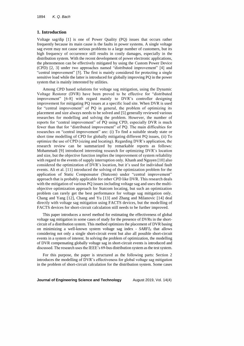
1894 K. Q. Bach

Journal of Engineering Science and Technology August 2019, Vol. 14(4)

1. Introduction

Voltage sag/dip [1] is one of Power Quality (PQ) issues that occurs rather

frequently because its main cause is the faults in power systems. A single voltage

sag event may not cause serious problems to a large number of customers, but its

high frequency of occurrence still results in costly damages, especially in the

distribution system. With the recent development of power electronic applications,

the phenomenon can be effectively mitigated by using the Custom Power Device

(CPD) [2, 3] under two approaches named “distributed improvement” [4] and

“central improvement” [5]. The first is mainly considered for protecting a single

sensitive load while the latter is introduced for globally improving PQ in the power

system that is mainly interested by utilities.

Among CPD based solutions for voltage sag mitigation, using the Dynamic

Voltage Restorer (DVR) have been proved to be effective for “distributed

improvement” [6-8] with regard mainly to DVR’s controller designing

improvement for mitigating PQ issues at a specific load site. When DVR is used

for “central improvement” of PQ in general, the problem of optimizing its

placement and size always needs to be solved and [5] generally reviewed various

researches for modelling and solving the problem. However, the number of

reports for “central improvement” of PQ using CPD, especially DVR is much

fewer than that for “distributed improvement” of PQ. The main difficulties for

researches on “central improvement” are: (i) To find a suitable steady state or

short time modelling of CPD for globally mitigating different PQ issues, (ii) To

optimize the use of CPD (sizing and locating). Regarding DVR’s application, the

research review can be summarized by remarkable reports as follows:

Mohammadi [9] introduced interesting research for optimizing DVR’s location

and size, but the objective function implies the improvement of system reliability

with regard to the events of supply interruption only. Khanh and Nguyen [10] also

considered the optimization of DVR’s location, but it’s used for individual fault

events. Ali et al. [11] introduced the solving of the optimization problem for the

application of Static Compensator (Statcom) under “central improvement”

approach that is probably applicable for other CPD like DVR. This research deals

with the mitigation of various PQ issues including voltage sag and uses the multi-

objective optimization approach for Statcom locating, but such an optimization

problem can rarely get the best performance for voltage sag mitigation only.

Chang and Yang [12], Chang and Yu [13] and Zhang and Milanovic [14] deal

directly with voltage sag mitigation using FACTS devices, but the modelling of

FACTS devices for short-circuit calculation still needs to be further improved.

This paper introduces a novel method for estimating the effectiveness of global

voltage sag mitigation in some cases of study for the presence of DVRs in the short-

circuit of a distribution system. This method optimizes the placement of DVR basing

on minimizing a well-known system voltage sag index - SARFIX that allows

considering not only a single short-circuit event but also all possible short-circuit

events in a system of interest. In solving the problem of optimization, the modelling

of DVR compensating globally voltage sag in short-circuit events is introduced and

discussed. The research uses the IEEE’s 69-bus distribution system as the test system.

For this purpose, the paper is structured as the following parts: Section 2

introduces the modelling of DVR’s effectiveness for global voltage sag mitigation

in the problem of short-circuit calculation for the distribution system. Some cases

A Novel Method for Global Voltage Sag Compensation in IEEE 69 . . . . 1895


of study for DVR application are introduced. Section 3 introduces the problem of

optimization where objective function, assumption and constraints are defined and

discussed. The modelling of DVR is built in the test system modelling for short-

circuit calculation. Finally, the results for different pre-set parameters of DVR are

analysed in Section 4.

2. Modelling of DVR with Limited Current for Short-circuit

Calculation in Distribution System

2.1. DVR’s basic modelling for voltage sag mitigation

DVR is a FACTS device that is connected in series with the load that needs to be

protected or with the source that generates PQ issues to limit its bad influence to

the power system operation. The description of the DVR in the steady-state

calculation is popularly given as a voltage source [3] connected in series with the

impedance of the branch as Fig. 1(a). In modelling, the power system for short-

circuit calculation, the method of bus impedance matrix is often used and such

DVR’s model of a series connected voltage source is difficult to be applied.

However, the problem can be eased by replacing the voltage source model with

Norton’s equivalent current source as shown in Fig. 1(b).

In power system modelling for steady-state calculation, Norton’s equivalent

current source model of the DVR can be represented as a load current at the output

node (j) and a current source at the input node (k) as shown in Fig. 2 [15].

It is noticed that the node k is the position where the voltage is compensated by

DVR. In the radial distribution system, node j is the node nearer to the source and

node k is the node farther to the source (i.e., nearer to the load side).

Fig. 1. Norton’s equivalent current source model for DVR. UDVR: Series voltage source of DVR, IDVR: Current injected by DVR,

ZDVR: Internal reactance of DVR, Zjk: Impedance of branch j-k.

Fig. 2. Model for DVR for steady state analysis.

1896 K. Q. Bach


2.2. Modelling of DVR for global voltage sag mitigation

2.2.1. Modelling test system in a short-circuit event

For modelling, the effectiveness of the DVRs for global voltage sag mitigation, the

paper introduces the application of the superposition principle according to the

Thevenin theorem for the problem of short-circuit calculation in distribution system

[10]. It is assumed that the initial state of the test system is the short-circuit without

the presence of DVRs. Thus, the system bus voltage can be calculated as follows:

[𝑈0] = [𝑍𝑏𝑢𝑠] × [I0] (1)

where:

[U0]: Initial bus voltage matrix (voltage sag at all buses during power system

short-circuit).

[I0]: Initial injected bus current matrix (short-circuit current).

[𝑈0] =

[ �̇�𝑠𝑎𝑔.1

⋮�̇�𝑠𝑎𝑔.𝑘

⋮�̇�𝑠𝑎𝑔.𝑛]

(2)

[𝐼0] =

[ 𝐼�̇�1

⋮𝐼�̇�𝑘

⋮𝐼�̇�𝑛]

(3)

[Zbus]: System bus impedance matrix calculated from the bus admittance matrix:

[Zbus]= [Ybus]-1. If the short-circuit is assumed to have fault impedance, we can add

the fault impedance to [Zbus].

With the presence of DVRs, according to Thevenin theorem, the bus voltage

equation system should be modified as follows [16]:

[𝑈] = [𝑍𝑏𝑢𝑠] × ([𝐼0] + [∆𝐼])

= [𝑍𝑏𝑢𝑠] × [𝐼0] + [𝑍𝑏𝑢𝑠] × [∆𝐼] = [𝑈0] + [∆𝑈] (4)

where:

[∆𝑈] = [𝑍𝑏𝑢𝑠] × [∆𝐼] (5)

or

[ ∆�̇�1

⋮∆�̇�𝑘

⋮∆�̇�𝑛]

= [Zbus] ×

[ ∆𝐼1̇⋮

∆𝐼�̇�⋮

∆𝐼�̇�]

(6)

Ui: Bus i voltage improvement (I = 1 n) after adding DVRs in the system.

Ii: Additional injected current to the bus i (I = 1 n) after adding the DVRs

in the system.



2.2.2. Voltage sag mitigation when placing a multiple of DVRs in system of

interest

It assumes that M is the set of m branches to connect to m DVRs (Fig. 3), a DVR

on a branch between bus j (near source side) and bus k (near load side) is

equivalently replaced by a current injected in bus k and a current going out from

bus j. From (6), the voltage of a bus i, is calculated as follows

∆�̇�𝑖 = ∑ 𝑍𝑖𝑗 × ∆𝐼�̇�𝑛𝑗=1 (7)

where:

∆𝐼�̇� = ∑ 𝑘𝑡.𝐷𝑉𝑅 × 𝑘𝑡.∗ × 𝐼𝑡.𝐷𝑉𝑅𝑡∈𝑇𝑗 (8)

Tj: Set of branches connected to bus j.

kt.DVR: Factor for placing DVR on the branch t. If the branch t is placed with

DVR, kt.DVR = 1. Otherwise, kt.DVR = 0.

kt.*: Factor for DVR’s voltage compensating position. If bus j is the voltage

compensating position by the DVR on the branch t, kt.* = +1. Otherwise, if bus j is

not the voltage compensating position by the DVR on the branch t, kt.* = -1.

It.DVR: Injected current by DVR on the branch t.

Note that for the distribution system with typical radial network configuration,

each bus is only connected with one branch toward the source. However, it is

possibly connected to more than one branch toward the load side (Fig. 4).

Therefore, if we define that the voltage compensating bus of the DVR coupled

branch is the bus toward the load side, each bus will definitely be the voltage

compensating position of not more than one DVR. In other words, m DVR coupled

branches have corresponded to m different buses of voltage compensation (marked

“*”). For m buses of voltage compensation by DVR, we have the condition of

voltage compensation as follows:

Fig. 3. System modelling with presence of m DVRs.

Fig. 4. System bus as voltage compensating position.

1898 K. Q. Bach


2.2.3. Modelling test system with presence of one DVR

Assuming a DVR is placed on the branch j-k. Basing on the DVR modelling in Fig.

2, in the matrix of additional injected bus current Eq. (6), there are only two

elements that do not equal to zero (Fig. 5). They are Ik = + IDVR and Ij = IDVR.

Other elements equal zero (Ii = 0 for i=1n, ij and ik).

Fig. 5. Test system modelling using [Zbus] with presence of one DVR.

Replace the above-assumed values of ∆𝐼𝑖 in Eq. (6), we have

∆�̇�𝑘 = 𝑍𝑘𝑘 × ∆𝐼�̇� + 𝑍𝑘𝑗 × ∆𝐼�̇� = (𝑍𝑘𝑘 − 𝑍𝑘𝑗) × 𝐼�̇�𝑉𝑅 (7)

According to the DVR modelling in Fig. 2, the voltage of bus k is compensated

up to the desired value. Khanh and Nguyen [10] proposed the desired value is 1

p.u. It means the bus k voltage is boosted by DVR from 𝑈𝑘0 = 𝑈𝑠𝑎𝑔.𝑘 up to Uk = 1

p.u. Therefore,

∆�̇�𝑘 = 1 − �̇�𝑠𝑎𝑔.𝑘 (8)

Replace Eqs. (8) into (7), we get 𝐼𝑘.𝐷𝑉𝑅∗ :

𝐼𝑘.𝐷𝑉𝑅∗ = ∆𝐼�̇� =

∆�̇�𝑘

𝑍𝑘𝑘−𝑍𝑘𝑗=

1−�̇�𝑠𝑎𝑔.𝑘

𝑍𝑘𝑘−𝑍𝑘𝑗 (9)

Then the comparison of IDVR calculated in Eq. (9) and a given IDVRmax is as follows:

If 𝐼𝑘.𝐷𝑉𝑅∗

calculated by Eq. (9) is not greater than a given IDVRmax, the voltage of

bus k is boosted up to 1 p.u. And the upgraded voltage for other bus i (I = 1

n; ik) in the test system can be calculated as follows:

∆�̇�𝑖 = 𝑍𝑖𝑘 × ∆𝐼�̇� + 𝑍𝑖𝑗 × ∆𝐼�̇� = (𝑍𝑖𝑘 − 𝑍𝑖𝑗) × 𝐼𝑘.𝐷𝑉𝑅∗ (10)

If 𝐼𝑘.𝐷𝑉𝑅∗ calculated by Eq. (9) is greater than IDVRmax, the voltage of bus k is

calculated as follows:

�̇�𝑘 = (𝑍𝑘𝑘 − 𝑍𝑘𝑗) × 𝐼�̇�𝑉𝑅𝑚𝑎𝑥 + �̇�𝑠𝑎𝑔.𝑘 < 1 𝑝. 𝑢. (11)

The upgraded voltage for other bus i (i = 1n; ik) in the test system can be

calculated as follows:

∆�̇�𝑖 = (𝑍𝑖𝑘 − 𝑍𝑖𝑗) × 𝐼�̇�𝑉𝑅𝑚𝑎𝑥 (12)

Finally, system bus voltages with the presence of DVR.

�̇�𝑖 = ∆�̇�𝑖 + �̇�𝑠𝑎𝑔.𝑖 (13)



2.2.4. Modelling test system with presence of two DVRs

In the case of a number of DVRs placed in the test system, for simply demonstrating

the algorithm, we consider the placement of two DVRs. Assuming DVR1 and

DVR2 are coupled on the branch j-k and branch e-f where bus k and bus f are the

voltage compensating positions respectively. The Norton’s equivalent circuits

using injected currents of DVRs are shown in Fig. 6.

Fig. 6. Test system modelling using [Zbus] with presence of two DVRs.

Therefore, Eq. (6) is written for this case of study as follows for the voltage

compensating buses k and f:

{∆�̇�𝑘 = (𝑍𝑘𝑘 − 𝑍𝑘𝑗) × 𝐼1̇.𝐷𝑉𝑅

∗ + (𝑍𝑘𝑓 − 𝑍𝑘𝑒) × 𝐼2̇.𝐷𝑉𝑅∗

∆�̇�𝑓 = (𝑍𝑓𝑘 − 𝑍𝑓𝑗) × 𝐼1̇.𝐷𝑉𝑅∗ + (𝑍𝑓𝑓 − 𝑍𝑓𝑒) × 𝐼2̇.𝐷𝑉𝑅

∗ (14)

Note that because of typically radial network configuration as said in 2.2.2., bus

e can be identical to bus j (buses toward the source side), however, bus f is never

identical to bus k (buses toward to load side).

Applying the voltage compensating condition to buses k and f, we have:

{∆�̇�𝑓 = 1 − �̇�𝑠𝑎𝑔.𝑓

∆�̇�𝑘 = 1 − �̇�𝑠𝑎𝑔.𝑘

(15)

Replace Eqs. (15) to (14) and solve the system of two equations, we have the

required DVR’s currents 𝐼1.𝐷𝑉𝑅∗ and 𝐼2.𝐷𝑉𝑅

∗ .

We verify the DVR’s maximum current and select I1.DVR and I2.DVR as step 2 in

2.2.2. Next, we calculate the bus i voltage increases as follows:

∆�̇�𝑖 = (𝑍𝑖𝑘 − 𝑍𝑖𝑗) × 𝐼1̇.𝐷𝑉𝑅 + (𝑍𝑖𝑓 − 𝑍𝑖𝑒) × 𝐼2̇.𝐷𝑉𝑅 (16)

For i=1n, ij, k, e, f.

And finally, we calculated all system bus voltages with the presence of two

DVRs as (10).

3. Problem Definition

3.1. Test system

For simplifying the introduction of the new method in the paper, the IEEE 69-bus

distribution feeder (Fig. 7) is used as the test system because it just features a balanced

1900 K. Q. Bach


three-phase distribution system, with three-phase loads and three-phase lines. This

system is large enough for testing the placement of one or a number of DVRs.

This research assumes base power to be 100 MVA. The base voltage is 11 kV.

The system voltage is 1 p.u. System impedance is assumed to be 0.1 p.u.

Fig. 7. IEEE 69-bus distribution system.

3.2. Short-circuit calculation

The paper only considers voltage sags caused by faults. Because the method

introduced in this paper considers SARFIX, we have to consider all possible fault

positions in the test system. However, to simplify the introduction of the new

method, we can consider only three-phase short-circuits. Other short-circuit types

can be taken similarly in the model if detailed calculation is needed.

Three-phase short-circuit calculation is performed using the method of bus

impedance matrix. The resulting bus voltage sags with and without the presence of

DVRs can be calculated for different cases of given influential parameters as

analysed in Section 4.

3.3. Problem of optimization

3.3.1. Objective function, assumptions and constraints

Reviewed publications in Part I suggests that for an application of power quality

solution, a cost-effect model can be introduced when the cost of power quality

solution (investment) and benefices from the resulting power quality mitigation are

addressed. However, for such a systematic solution as global voltage sag mitigation

by DVRs, its benefice is hard to quantify. Therefore, in this research, the application

of DVRs for global voltage sag mitigation is performed that based on the problem of

optimizing the location of one or a multiple of DVRs in the test system where the

objective function is only to minimize the System Average RMS Variation Frequency

Index - SARFIX where X is a given RMS voltage threshold [17].

𝑆𝐴𝑅𝐹𝐼𝑋 =∑ 𝑛𝑖.𝑋

𝑛𝑖=1

𝑛⇒ Min (17)



where:

ni.X: The number of voltage sags lower than X% of the load i in the test

system.

n: The number of loads (assuming all buses in the system).

Therefore, this research accepts an important assumption that the problem of

optimization does not take account of any costs for power quality investment as

well as resulting benefices. In this problem, for an in-advance given a number of

DVRs with a given limited current, we need to find the optimal scenarios of DVR

placement in order to achieve the best performance of global voltage sag mitigation.

That is why SARFIX is used as an objective function.

For a given fault performance (fault rate distribution rf) of a given system and a

given threshold X, SARFIX calculation is described as the block diagram in Fig. 8

[18]. For SARFIX calculation in Fig. 8, one important thing is the calculating all bus

voltages of the system of interest without or with the presence of a number of DVRs

in a certain scenario of placement (blocks (*) and (**)). These calculations are newly

introduced in subsection 2.2.2.

Fig. 8. Block-diagram of SARFIX calculation.

1902 K. Q. Bach


For this problem of optimization, the main variable is the scenario of positions

(branches) where DVRs are placed. Because of radial network topology, a

distribution system with n buses has n-1 branches. For the 69-bus test system, we

have 68 branches. If m DVRs are considered, the total scenarios of DVR placement

to be tested are as follows:

𝑇𝑚 = 𝐶𝑛−1𝑚 =

(𝑛−1)!

𝑚!×(𝑛−1−𝑚)!=

68!

𝑚!×(68−𝑚)! (18)

For example, if we consider the placement of one DVR in the test system, we

have m = 1 and total scenarios for placing this DVR is 𝑇1 = 𝐶681 =

68!

1!×(68−1)!= 68.

Each candidate scenario to be tested is the bus number k, (k = 168).

If we consider the placement of two DVRs in the test system, we have m = 2 and

the total scenarios for placing these two DVRs is 𝑇2 = 𝐶682 =

68!

2!×(68−2)!= 2278.

The problem of optimization has no constraint, but there’re two important

assumptions: Firstly, a DVR’s parameter, which is the limited current of DVR is

in-advance given. The modelling about how DVR with a limited current can

compensate globally voltage sag is introduced in subsection 2.2.2. Secondly, the

DVR’s operation is assumed [6-8] that DVR only works if it is placed on the branch

that is not a part of fault current carrying path (from the source to the fault position).

In this case, the bypass switch is actually closed to disable DVR’s operation.

3.3.2. Problem-solving

For such a problem of optimization, with pre-set parameters (X%, and DVR’s

limited current), the objective function - SARFIX is always determined for any

candidate scenarios of DVR’s placement in Tm. Therefore, we use the method of

direct search and test all scenarios of DVR positions. The block-diagram of solving

this problem in Matlab is given in Fig. 9. In this block-diagram, firstly, the set M

of Tm candidate scenarios of placement of m DVRs Eq. (18) is listed. Then,

according to the said method of direct search, for each candidate scenario k (kM),

the corresponding SARFIX is calculated.

Calculating SARFIX of the test system with and without the presence of DVRs is

performed as Figs. 8 and 10. With the presence of m DVRs coupled on m branches,

as discussed in subsection 2.2.2., we have m* buses of voltage compensation by

DVR. Figure 8 shows the algorithm starting with verifying of branch t.

The (t = 1 m) connected with DVR is part of a fault current carrying path or

not. If it’s the case, DVR on this branch is disabled by the bypass switch and we

have It.DVR = 0. After that, the condition of voltage compensation by DVR is applied

for above said m* buses to calculate the required 𝐼𝑡.𝐷𝑉𝑅∗ . Then, DVR’s maximum

current is checked to finally calculate the system bus voltage as (10).

In the block-diagram, input data that can be seen as the above said pre-set

parameters. The “postop” is the intermediate variable that fixes the scenario of DVR’s

location corresponding to the minimum SARFIX. The initial solution of objective

function Min equals B, which is a big enough value (e.g., B = 69) for starting the

search process. The scenarios for different parameters of fault events are considered.



Fig. 9. Block-diagram of solving

problem of optimization.

Fig. 10. Block-diagram of calculating

system voltage with presence of DVRs.

4. Result Analysis

4.1. Preset parameters

The research considers the following pre-set parameters:

For calculating SARFIX, the fault performance, which is fault rate distribution,

is assigned to all fault positions. According to Khanh et al. [18], just for

introducing the method, the paper assumingly uses the uniform fault

distribution (simplest fault distribution modelling) and fault rate equals 1 time

per period of time for each fault position (assumed at each bus).

For RMS voltage threshold, the paper only considers voltage sags, so X is given

as 90, 80, 70, 50% of Un.

For DVR’s limited current, the paper considers IDVRmax = 0.1, 0.5, 1 and 1.5 p.u.

4.2. First case of study: Placing one DVR in test system

The simplest case is that with one DVR placed in the test system. In solving the

problem of optimization considering the above said pre-set parameters, results are

step-by-step introduced for better analysis and discussion. For a case of pre-set

parameters, we initially consider sag X =80%, IDVRmax = 0.5 p.u. For calculating

SARFIX of the test system with the presence of one DVR at a certain location, we

1904 K. Q. Bach


have to collect the sag frequency for all load buses (69 buses) caused by all possible

fault positions (69 buses). For each fault position, firstly, the algorithm will check

to see whether the DVR is on the fault current carrying path or not. For example, if

the fault occurs at the bus 57, branches on the path from bus 1 to bus 57 (red marked

in Fig. 11) are the locations where DVR is disabled if it is placed on these branches.

If DVR is not on the fault current carrying path, for example, DVR is on branch

15 (between bus 15 and bus 16), the bus voltage improvement is shown on Fig. 12

to illustrate the performance of DVR’s model as introduced in subsections 2.1 and

2.2. With the DVR placed on branch 15, the voltage at bus 16 is boosted to 1 p.u.

and the required injected current from DVR is 1.4514 p.u., which is quite large.

The buses from bus 16 to the end of this lateral tap (bus 27) are all compensated to

1 p.u. Other bus voltages remain unchanged. However, with regard to the DVR’s

limited current, for example, we assumed IDVRmax = 0.5 p.u., the voltages from bus

16 to bus 27 are just upgraded as the red line (0.8397 p.u.) in Fig. 12. For the X =

80%, 40 buses experiencing voltage sag are counted. However, with the presence

of DVR, only 28 buses having the voltage lower than 80% are counted.

Fig. 11. Checking locations where DVR

is disabled for a give fault position.

Fig. 12. Bus voltage without and with DVR placed

on branch 15 (15-16) for short-circuit at bus 57.

Similarly, the algorithm (as shown in Fig. 8) calculates the frequency of voltage

sag for the magnitude X (resulted by all possible fault positions) at all buses and



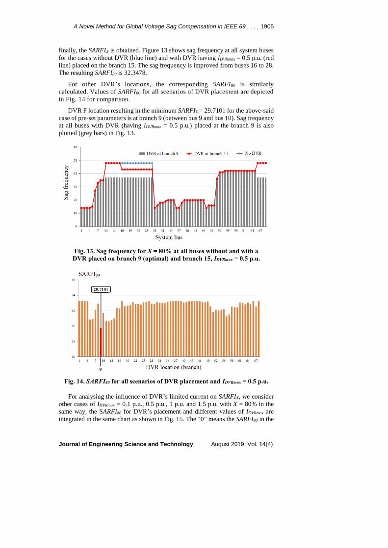
finally, the SARFIX is obtained. Figure 13 shows sag frequency at all system buses

for the cases without DVR (blue line) and with DVR having IDVRmax = 0.5 p.u. (red

line) placed on the branch 15. The sag frequency is improved from buses 16 to 28.

The resulting SARFI80 is 32.3478.

For other DVR’s locations, the corresponding SARFI80 is similarly

calculated. Values of SARFI80 for all scenarios of DVR placement are depicted

in Fig. 14 for comparison.

DVR F location resulting in the minimum SARFIX = 29.7101 for the above-said

case of pre-set parameters is at branch 9 (between bus 9 and bus 10). Sag frequency

at all buses with DVR (having IDVRmax = 0.5 p.u.) placed at the branch 9 is also

plotted (grey bars) in Fig. 13.

Fig. 13. Sag frequency for X = 80% at all buses without and with a

DVR placed on branch 9 (optimal) and branch 15, IDVRmax = 0.5 p.u.

Fig. 14. SARFI80 for all scenarios of DVR placement and IDVRmax = 0.5 p.u.

For analysing the influence of DVR’s limited current on SARFIX, we consider

other cases of IDVRmax = 0.1 p.u., 0.5 p.u., 1 p.u. and 1.5 p.u. with X = 80% in the

same way, the SARFI80 for DVR’s placement and different values of IDVRmax are

integrated in the same chart as shown in Fig. 15. The “0” means the SARFI80 in the

1906 K. Q. Bach


case without DVR. Obviously, a higher limited current produces a better (smaller)

SARFIX improvement.

For considering the improvement of SARFIX for different levels of voltage sag

magnitude X, the results of SARFIX for X = 50%, 70%, 80% and 90% with IDVRmax = 0.5

p.u. are shown in the Fig. 16. The “0” means the SARFIX without DVR. Finally,

remarkable results for all pre-set parameters are summarized in Table 1. We can see

that the SARFIX improvement is generally not big for DVR because DVR can only

compensate for the voltage of the buses from the DVR’s location towards to load side.

Fig. 15. SARFIX=80% for all scenarios of DVR

placement, IDVRmax = 0.1, 0.2, 0.3, 0.5 p.u.

Fig. 16. SARFIX=80% for all scenarios of DVR placement for different

voltage sag magnitude (50%, 70%, 80% and 90%), IDVRmax = 0.5 p.u.

Table 1. Results for using one DVR placement.

Results IDVRmax (p.u.)

c 0.1 0.5 1 1.5 X = 50%

minSARFIX 21.7971 21.4783 19.3188 16.5797 16.5797

DVR branch 9 56 11 6

X = 70%

minSARFIX 27.6957 27.1739 25.4638 21 21

DVR branch 56 9 9 9

X = 80%

minSARFIX 33.2174 31.6232 29.7101 26.0435 24.9275

DVR branch 9 9 12 9

X = 90%

minSARFIX 42.7101 9 36.6522 33.7826 31.2319

DVR branch 22 9 13 9



4.3. Second case of study: Placing two (multiple) DVRs in test system

To illustrate the algorithm’s performance for the case of a number of DVRs placed

in the test system, we consider to optimally select the locations of two DVRs. In

solving the problem of optimization considering pre-set parameters as Section 4.1,

results are also step-by-step introduced for better analysis and discussion.

Firstly, we also start to consider sag X = 80%. We consider a candidate scenario

of locating two DVRs on branch 15 and branch 65 (Fig. 17). If short-circuit position

is still bus 57, the required currents for DVRs for boosting the voltage at DVR’s

location to 1 p.u. are IDVR1 = 1.1451 p.u. and IDVR2 = 1.4294 p.u. respectively, which

are quite high. If we consider the DVR’s limited current IDVRmax = 0.5 p.u., the bus

voltages are mitigated as shown in Fig. 18.

With regard to sag voltage level X = 80%, without DVR, there are 40 buses

having the voltage lower than X. This figure reduces to 26 buses for placing DVRs

on branches 15 and 65.

Fig. 17. Checking locations where

DVRis disabled for a give fault position.

Fig. 18. System bus voltage without and with 2 DVRs placed

on branches 15 (15-16) and 65 (11-66) for short-circuit at bus 57.

1908 K. Q. Bach


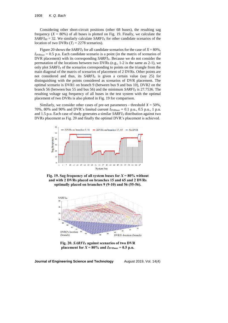
Considering other short-circuit positions (other 68 buses), the resulting sag

frequency (X = 80%) of all buses is plotted on Fig. 19. Finally, we calculate the

SARFI80 = 32. We similarly calculate SARFIX for other candidate scenarios of the

location of two DVRs (T2 = 2278 scenarios).

Figure 20 shows the SARFIX for all candidate scenarios for the case of X = 80%,

IDVRmax = 0.5 p.u. Each candidate scenario is a point (in the matrix of scenarios of

DVR placement) with its corresponding SARFIX. Because we do not consider the

permutation of the locations between two DVRs (e.g., 1-2 is the same as 2-1), we

only plot SARFIX of the scenarios corresponding to points on the triangle from the

main diagonal of the matrix of scenarios of placement of 2 DVRs. Other points are

not considered and thus, its SARFIX is given a certain value (say 25) for

distinguishing with the points considered as scenarios of DVR placement. The

optimal scenario is DVR1 on branch 9 (between bus 9 and bus 10), DVR2 on the

branch 56 (between bus 55 and bus 56) and the minimum SARFIX is 27.7536. The

resulting voltage sag frequency of all buses in the test system with the optimal

placement of two DVRs is also plotted in Fig. 19 for comparison.

Similarly, we consider other cases of pre-set parameters - threshold X = 50%,

70%, 80% and 90% and DVR’s limited current IDVRmax = 0.1 p.u., 0.5 p.u., 1 p.u.

and 1.5 p.u. Each case of study generates a similar SARFIX distribution against two

DVRs placement as Fig. 20 and finally the optimal DVR’s placement is achieved.

Fig. 19. Sag frequency of all system buses for X = 80% without

and with 2 DVRs placed on branches 15 and 65 and 2 DVRs

optimally placed on branches 9 (9-10) and 56 (55-56).

Fig. 20. SARFIX against scenarios of two DVR

placement for X = 80% and IDVRmax = 0.5 p.u.



Remarkable results are summarised in Table 2. We can see again, the larger

IDVRmax results in better improvement of SARFIX. For many scenarios of pre-set

parameters, the optimal placement takes branch 9 and branch 56 that is in the

middle of long feeders. Higher threshold X results in higher SARFIX but the

improvement of SARFIX with different DVR’s limited current is the same.

Table 2. Remarkable results for two DVR placement.

Results IDVRmax (p.u.) No DVR 0.1 0.5 1 1.5

X = 50%

minSARFIX 21.7971 21.3478 16.9275 14.1014 14.1014

DVR placement

(branch)

DVR1 9 12 11 11

DVR2 56 56 56 56

X = 70%

minSARFIX 27.6957 26.8551 23.8986 17.6087 17.6087

DVR placement

(branch)

DVR1 9 9 9 9

DVR2 56 56 56 56

X = 80%

minSARFIX 33.2174 30.7101 27.7536 21.7391 20.6232

DVR placement

(branch)

DVR1 9 9 12 9

DVR2 56 56 56 56

X = 90%

minSARFIX 42.7101 37.8116 32.6087 27.3913 24.8406

DVR placement

(branch)

DVR1 9 9 13 9

DVR2 56 56 56 56

5. Conclusion

This paper introduces a new method for global voltage sag mitigation by using a

number of DVRs in the distribution system where the effectiveness of global

voltage sag mitigation by DVRs for the case of limited maximum current is

modelled using Thevenin’s superposition theorem in short-circuit calculation of

power distribution systems. This method allows us to consider the DVR’s

effectiveness of voltage sag mitigation not only for event index but also for site and

system indices. As a result, the optimal scenario of DVR placement is obtained by

minimizing the resulting SARFIX with regard to pre-set parameters including the

voltage threshold X and the DVR’s maximum injected current. The paper also

considers the case of using a number of DVRs for global voltage sag mitigation

that is applicable for large size distribution systems.

For the purpose of introducing the method, some assumptions are accompanied

by the type of short-circuiting and the fault rate distribution. For real applications, the

method can easily include the real fault rate distribution as well as all types of short-

circuiting. DVR’s effectiveness of global voltage sag mitigation is relatively limited

as DVR can only compensate the voltage of buses from the DVR’s location toward

load side and it is also disabled if it is coupled on the fault current carrying path.

The method of optimizing the DVR placement only considers how to get the best

outcome of an in-advance given a number of DVRs without considering DVR

investment. That is because the cost-effective model cannot be built for such a

systematic solution as global voltage sag mitigation. Further research should address

this limitation by trying to quantify the benefice of global voltage sag mitigation.

1910 K. Q. Bach


Nomenclatures

IDVR.max DVR’s limited current, p.u.

I0 Initial injected bus current matrix (Short-circuit current), p.u.

Ifk Fault current at bus k, p.u.

𝐼𝑘.𝐷𝑉𝑅∗ Injected current by DVR on the branch k, (kM) that boosts the

voltage of bus k to 1 p.u.

It.DVR Injected current by DVR on the branch t, p.u.

kt.* Factor for DVR’s voltage compensating position

kt.DVR Factor for placing DVR on branch t

M Set of m branches to connect to m DVRs

m* Buses of voltage compensation by DVR

SARFIX System average RMS variation frequency index

Tj Set of branches connected to bus j

Tm Total scenarios of DVR placement to be tested

U Bus voltage matrix after adding DVRs in system, p.u.

U0 Initial bus voltage matrix (Voltage sag at all buses

during power system short-circuit), p.u.

Usag.i Voltage sag at bus i during power system short-circuit

X RMS voltage threshold, %

Zbus System bus impedance matrix calculated from bus admittance

matrix, p.u.

Greek Symbols

I Additional injected current matrix by DVR, p.u.

Ii Additional injected current to the bus i after adding DVRs

in system, p.u.

U Bus voltage improvement matrix after adding the

DVRs in system, p.u.

Ui Bus i voltage improvement after adding DVRs in system, p.u.

Abbreviations

DVR Dynamic Voltage Restorer

References

1. IEEE. (2009). IEEE Recommended practice for monitoring power quality.

IEEE Standards 1159-2009.

2. Ghosh, A; and Ledwich, G. (2002). Power quality enhancement using custom

power devices. Norwell, Massachusetts, United States of America: Kluwer

Academic Publishers.

3. Bollen, M.H. (2000). Understanding power quality problems: Voltage sags

and interruptions. New York, United States of America: Wiley IEEE Press.

4. Tanti, D.K.; Verma, M.K.; Singh, B.; and Mehrotra, O.N. (2012). Optimal

placement of custom power devices in power system network to mitigate

voltage sag under faults. International Journal of Power Electronics and Drive

System, 2(3), 267-276.

5. Farhoodnea, M; Mohamed, A; Shareef, H.; and Zayanderoodi, H. (2012). A

comprehensive review of optimization techniques applied for placement and



sizing of custom power devices in distribution networks. Przegląd

Elektrotechniczny, 88(11a), 261-265.

6. Pal, R.; and Gupta, S. (2015). State of the art: Dynamic voltage restorer for

power quality improvement. Electrical and Computer Engineering: An

International Journal (ECIJ), 4(2), 79-98.

7. Omar, R.; Rahim, N.A.; and Sulaiman, M. (2011). Dynamic voltage restorer

application for power quality improvement in electrical distribution system: An

Overview. Australian Journal of Basic and Applied Sciences, 5(12), 379-396.

8. Chaudhary, S.H.; and Gangil, G. (2013). Mitigation of voltage sag/swell using

dynamic voltage restorer (DVR). IOSR Journal of Electrical and Electronics

Engineering (IOSR-JEEE), 8(4), 21-38.

9. Mohammadi, M. (2013). Voltage dip rating reduction based optimal location of

DVR for reliability improvement of electrical distribution system. International

Research Journal of Applied and Basic Sciences, 4(11), 3493-3500.

10. Khanh, B.Q.; and Nguyen, M.V. (2018). Using the Norton’s equivalent circuit

of DVR in optimizing the location of DVR for voltage sag mitigation in

distribution system. GMSARN International Journal, 12(3), 139-144.

11. Ali, M.A.; Fozdar, M.; Niazi, K.; and Phadke, A.R. (2015). Optimal placement

of static compensators for global voltage sag mitigation and power system

performance improvement. Research Journal of Applied Sciences,

Engineering and Technology, 10(5), 484-494.

12. Chang, C.S.; and Yang, S.W. (2000). Tabu search application for optimal

multiobjective planning of dynamic voltage restorer. Proceedings of IEEE

Power Engineering Society Winter Meeting (Volume 4). Singapore, 2751-2756.

13. Chang, C.S.; and Yu, Z. (2004). Distributed mitigation of voltage sag by

optimal placement of series compensation devices based on stochastic

assessment. IEEE Transaction on Power Systems, 19(2), 788-795.

14. Zhang, Y.; and Milanovic, J.V. (2010). Global voltage sag mitigation with

FACTS-based devices. IEEE Transaction on Power Delivery, 25(4), 2842-2850.

15. Ratniyomchai, T.; and Kulworawanichpong T. (2006). Steady-state power

flow modeling for a dynamic voltage restorer. Proceedings of 5th WSEAS,

Conference on Applications of Electrical Engineering (ICAEE). Prague, Czech

Republic, 6-11.

16. Grainger, J.J.; and Stevenson W.D. (1994). Power system analysis. New York,

United States of America: McGraw-Hill.

17. IEEE. (2014). Guide for voltage sag indices. IEEE Standards 1564-2014.

18. Khanh, B.Q.; Won, D.-J.; and Moon, S. (2008). Fault distribution modeling

using stochastic bivariate models for prediction of voltage sag in distribution

systems. IEEE Transactions on Power Delivery, 23(1), 347-354.

a novel method for global voltage sag compensation …

Documents