a permutation approach to validation - computer sciencemagdon/talks/permutationvalsdm2010.pdf · a...

A Permutation Approach to Validation

M. Magdon-Ismail, Konstantin Mertsalov

Siam Conference on Data Mining (SDM)April 30 2010

Example: Learning Male Vs. Female Faces

Male Female

Learned rule: “roundish face or long hair is female”

ein = 218 ≈ 11%

eout =??

It has been known since the early days that ein ≪ eout.

[Larson, 1931; Wherry, 1931, 1951; Katzell, 1951; Cureton, 1951; Mosier, 1951; Stone, 1974]

c© Magdon-Ismail : Mertsalov. 30 April, 2010. 1–2

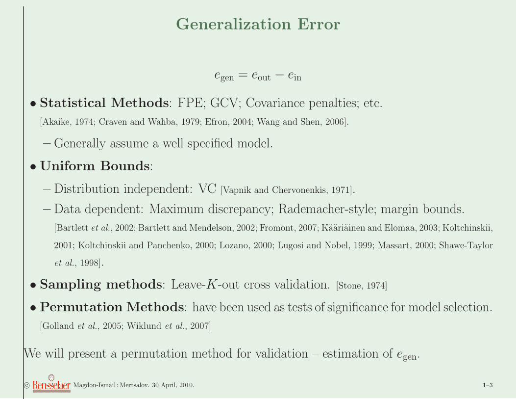
Generalization Error

egen = eout − ein

• Statistical Methods: FPE; GCV; Covariance penalties; etc.

[Akaike, 1974; Craven and Wahba, 1979; Efron, 2004; Wang and Shen, 2006].

– Generally assume a well specified model.

•Uniform Bounds:

– Distribution independent: VC [Vapnik and Chervonenkis, 1971].

– Data dependent: Maximum discrepancy; Rademacher-style; margin bounds.

[Bartlett et al., 2002; Bartlett and Mendelson, 2002; Fromont, 2007; Kaariainen and Elomaa, 2003; Koltchinskii,

2001; Koltchinskii and Panchenko, 2000; Lozano, 2000; Lugosi and Nobel, 1999; Massart, 2000; Shawe-Taylor

et al., 1998].

• Sampling methods: Leave-K-out cross validation. [Stone, 1974]

• Permutation Methods: have been used as tests of significance for model selection.

[Golland et al., 2005; Wiklund et al., 2007]

We will present a permutation method for validation – estimation of egen.


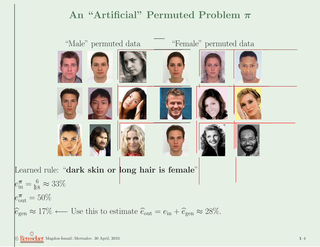
An “Artificial” Permuted Problem π

“Male” permuted data “Female” permuted data

Learned rule: “dark skin or long hair is female”

eπ

in = 618≈ 33%

eπ

out = 50%

egen ≈ 17% ←− Use this to estimate eout = ein + egen ≈ 28%.


Permutation Method for Regression

Real Data Permuted Data

Linear Fit Quartic Fit

ein = 0.02 ein = 0.002

eout = 0.11 eout = 0.256

egen = 0.08 egen = 0.254

eout = 0.07 eout = 0.192

Linear Fit Quartic Fit

average(einπ) = 0.12 average(ein

π) = 0.05

average(eoutπ) = 0.17 average(eout

π) = 0.24

average(egen) = 0.05 average(egen) = 0.19


The Permutation Method For Validation

1. Fit the real data to obtain ein(g).

2. Permute the y values using permutation π.

(a) Fit the permuted data to obtain gπ

(b) Compute the generalization error on the artificial permuted problem.

Theorem 1. eπ

out(gπ) = s2

y +1

n

n∑

i=1

(gπ(xi)− y)2.

Theorem 2. eπ

gen(gπ) =

2

n

n∑

i=1

(yπi− y)gπ(xi)

(Twice the (spurious) correlation between gπ and yπ.)

3. Repeat (say 100 times) to get an average(egen).

4. Estimate the out-sample error

eout = ein + egen.


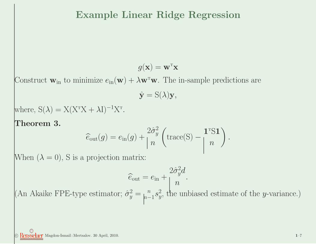
Example Linear Ridge Regression

g(x) = wtx

Construct win to minimize ein(w) + λwtw. The in-sample predictions are

y = S(λ)y,

where, S(λ) = X(XtX + λI)−1Xt.

Theorem 3.

eout(g) = ein(g) +2σ2

y

n

(trace(S)−

1tS1

n

).

When (λ = 0), S is a projection matrix:

eout = ein +2σ2

yd

n.

(An Akaike FPE-type estimator; σ2y = n

n−1s2y, the unbiased estimate of the y-variance.)


Validation Results

0.364

0.366

0.368

0.37

0.372

0.374

0.376

0.378

0.38

0.382

0.384

0 50 100 150 200 250 300 350 400 450 500

Exp

. Out

-of-

sam

ple

erro

r

Number of leaves

eouteCV

eperm

0.36

0.38

0.4

0.42

0.44

0.46

0.48

0.5

0 20 40 60 80 100

Exp

. Out

-of-

sam

ple

erro

r

k

eouteCV

eperm

(a) LOO-CV vs. Permutation (DT) (b) LOO-CV vs. Permutation (k-NN).

2 4 6 8 10

0.7

0.75

0.8

0.85

Order of Model (K)

Exp

ecte

d O

ut−

of−

Sam

ple

Err

or

eout

eCV

eperm

eVC

eFPE

2 4 6 8

0.7

0.75

0.8

0.85

Regularization Parameter (λ / N)

Exp

ecte

d O

ut−

of−

Sam

ple

Err

or

eout

eCV

eperm

eVC

eFPE

(a) Different Polynomial Order. (b) Different Regularization Parameter.


Model Selection – Simulated Setting

λ Selection

Validation Order Selection Unregularized Regularized

Estimate Regret Avg Order Regret Avg. λN

Regret

LOO-CV 540 9.29 18.8 23.1 0.44

Perm. 185 7.21 5.96 9.57 0.39

VC 508 5.56 3.50 125 0.42

FPE 9560 11.42 51.3 18.1 0.87

Noise(%) LOO-CV Perm. Rad.

5 0.30 0.28 0.28

10 0.28 0.27 0.27

15 0.28 0.25 0.25

20 0.28 0.26 0.26

25 0.26 0.25 0.25

30 0.24 0.24 0.24


Model Selection – Real Data

Data Decision Trees k-Nearest Neighbor

LOO-CV Perm. Rad. LOO-CV Perm. Rad.

Abalone 0.05 0.02 0.02 0.04 0.04 0.04

Ionosphere 0.17 0.16 0.17 0.17 0.70 0.83M.Mass 0.09 0.05 0.05 0.09 0.11 0.11

Parkinsons 0.24 0.34 0.41 0.25 0.33 0.43Pima Diabetes 0.09 0.07 0.07 0.11 0.11 0.14

Spambase 0.07 0.06 0.07 0.19 0.43 0.55Transfusion 0.10 0.08 0.09 0.09 0.12 0.19WDBC 0.20 0.23 0.34 0.21 0.34 0.51

Diffusion 0.04 0.03 0.02 0.04 0.06 0.03Simulated 0.16 0.15 0.15 0.21 0.21 0.21

Learning episodes limited to 10

Data Decision Trees k-Nearest NeighborLOO-CV 10-fold Perm. Rad. LOO-CV Perm. Rad.

Abalone 0.12 0.13 0.02 0.02 0.24 0.09 0.12Ionosphere 0.24 0.21 0.18 0.19 0.49 0.75 0.84

M.Mass 0.23 0.13 0.06 0.06 0.15 0.11 0.12Parkinsons 0.25 0.31 0.34 0.40 0.34 0.32 0.44

Pima Diabetes 0.18 0.18 0.07 0.07 0.16 0.12 0.15Spambase 0.28 0.09 0.07 0.07 0.44 0.43 0.54

Transfusion 0.19 0.13 0.08 0.09 0.17 0.12 0.19WDBC 0.31 0.40 0.24 0.37 0.55 0.33 0.50

Diffusion 0.13 0.04 0.03 0.02 0.09 0.06 0.04


What Have We Learned?

• To estimate eout: hard to beat LOO-CV (in expectation).

•Model selection: need good estimate, but also stable.

• VC – ultra stable, very conservative.

• LOO-CV – very unstable, in general good, but can be a disaster.

• Permutation Method – Good blend.

– To have low egen, the method must generalize well on random permutations which

have similar structure to the data. This induces stability.

– Seems to be better than Rademacher, which is of a similar flavor: the permutation

preserves more of the structure of the data, while at the same time being stable.


. . . And Now the Theory: Permutation Complexity

Permutation Complexity

Pin(H|D) = Eπ

[maxh∈H

1

n

n∑

i=1

yπih(xi)

].

We consider random permutations π of the y values.

Some function in your hypothesis set achieves a maximum (spurious) correlation with

this random permutation.

The expected value of this spurious correlation is the permutation complexity.

• data dependent.

• can be computed by empirical error minimization.

[Rademacher complexity is similar except that it chooses yi independently and uniformly in {±1}.]


Permutation Complexity Uniform Bound

Theorem 4.

eout(g) ≤ ein(g) + 4Pin(H|D) + O(√

1n

ln 1δ

),

(∗)= ein(g) + 2egen(H|D) + 4y Eπ [gπ] + O

(√1n

ln 1δ

).

(∗) is for empirical risk minimization (ERM).

Up to a small “bias term”, egen bounds eout (for ERM).

The bound is uniform, and data dependent.

Practical “consequence”: we are “justified” in using the permutation estimate.


Proof

•We now have tools for i.i.d. sampling: McDiarmid’s Inequality [McDiarmid, 1989].

• The main difficulty: permutation sampling is not independent.

• The insight is to use multiple ghost samples to “unfold” this dependence.

• . . . one still has to go through a few technical details, but then you have it.


Wrapping Up

• The permutation estimate is easy to compute numerically - all you do is run the

algorithm on randomly permuted data.

• Can be used for classification or regression.

• In some cases (linear ridge regression), can get analytical form.

• Achieves a good blend (practically) between the conservative VC bound and the

highly unstable LOO-CV.

• Similar but slightly superior (in practice) to Rademacher penalties.

• . . . its only the begining.

Thank You! Questions?

Bibliography

Akaike, H. (1974). A new look at the statistical model identification. IEEE Trans. Aut. Cont., 19, 716–723.

Bartlett, P. L. and Mendelson, S. (2002). Rademacher and gaussian complexities: Risk bounds and structural results. Journal of Machine

Learning Research, 3, 463–482.

Bartlett, P. L., Boucheron, S., and Lugosi, G. (2002). Model selection and error estimation. Machine Learning , 48, 85–113.

Craven, P. and Wahba, G. (1979). Smoothing noisy data with spline functions. Numerische Mathematik , 31, 377–403.

Cureton, E. E. (1951). Symposium: The need and means of cross-validation: II approximate linear restraints and best predictor weights.Education and Psychology Measurement , 11, 12–15.

Efron, B. (2004). The estimation of prediction error: Covariance penalties and cross-validation. Journal of the American Statistical Association,99(467), 619–632.

Fromont, M. (2007). Model selection by bootstrap penalization for classification. Machine Learning , 66(2-3), 165–207.

Golland, P., Liang, F., Mukherjee, S., and Panchenko, D. (2005). Permutation tests for classification. Learning Theory , pages 501–515.

Kaariainen, M. and Elomaa, T. (2003). Rademacher penalization over decision tree prunings. In In Proc. 14th European Conference on

Machine Learning , pages 193–204.

Katzell, R. A. (1951). Symposium: The need and means of cross-validation: III cross validation of item analyses. Education and Psychology

Measurement , 11, 16–22.

Koltchinskii, V. (2001). Rademacher penalties and structural risk minimization. IEEE Transactions on Information Theory , 47(5), 1902–1914.

Koltchinskii, V. and Panchenko, D. (2000). Rademacher processes and bounding the risk of function learning. In E. Gine, D. Mason, andJ. Wellner, editors, High Dimensional Prob. II , volume 47, pages 443–459.

Larson, S. C. (1931). The shrinkage of the coefficient of multiple correlation. Journal of Education Psychology , 22, 45–55.

Lozano, F. (2000). Model selection using rademacher penalization. In Proc. 2nd ICSC Symp. on Neural Comp.

Lugosi, G. and Nobel, A. (1999). Adaptive model selection using empirical complexities. Annals of Statistics , 27, 1830–1864.

1-17

BIBLIOGRAPHY BIBLIOGRAPHY

Massart, P. (2000). Some applications of concentration inequalities to statistics. Annales de la Faculte des Sciencies de Toulouse, X, 245–303.

McDiarmid, C. (1989). On the method of bounded differences. In Surveys in Combinatorics, pages 148–188. Cambridge University Press.

Mosier, C. I. (1951). Symposium: The need and means of cross-validation: I problem and designs of cross validation. Education and Psychology

Measurement , 11, 5–11.

Shawe-Taylor, J., Bartlett, P. L., Williamson, R. C., and Anthony, M. (1998). Structural risk minimization over data dependent hierarchies.IEEE Transactions on Information Theory , 44, 1926–1940.

Stone, M. (1974). Cross validatory choice and assessment of statistical predictions. Journal of the Royal Statistical Society , 36(2), 111–147.

Vapnik, V. N. and Chervonenkis, A. (1971). On the uniform convergence of relative frequencies of events to their pr obabilities. Theory of

Probability and its Applications , 16, 264–280.

Wang, J. and Shen, X. (2006). Estimation of generalization error: random and fixed inputs. Statistica Sinica, 16, 569–588.

Wherry, R. J. (1931). A new formula for predicting the shrinkage of the multiple correlation coefficient. Annals of Mathematical Statistics,2, 440–457.

Wherry, R. J. (1951). Symposium: The need and means of cross-validation: III comparison of cross validation with statistical inference ofbetas and multiple r from a single sample. Education and Psychology Measurement , 11, 23–28.

Wiklund, S., Nilsson, D., Eriksson, L., Sjostrom, M., Wold, S., and Faber, K. (2007). A randomization test for pls component selection.Journal of Chemometrics, 21(10,11).


a permutation approach to validation - computer sciencemagdon/talks/permutationvalsdm2010.pdf · a...

Documents