1

A Phasor Description of the Stirling Cycle

David M. BERCHOWITZ

Global Cooling Inc., 6000 Poston Rd., Athens Ohio, USA, dberchowitz@globalcooling.com Keywords: Stirling, thermodynamics, phasors

ABSTRACT

A phasor representation of the Stirling cycle process is presented. This includes volume

variations, mass flows and heat transfer. The resulting pressure phasors are linked to free-piston dynamics that include the motor or alternator. The phasor analysis provides general simplifications that lead directly to a number of useful results that are not obvious from conventional approaches. These include the relationship of the displacer drive area to the flow losses and the processes that contribute to the regenerator performance. 1. INTRODUCTION

The mathematical description of the Stirling cycle has usually taken the form of simple

discrete processes [1] or a continuous process based on average conditions at different locations in the machine [2] [3]. The cycle is of course not discrete and most continuous process methods do not offer a clear, succinct thermodynamic description that allows inclusion of fundamental losses. What is needed is an an approach that describes the cycle accurately enough to understand the real world consequences of implementation. The standard Schmidt or isothermal analysis, though providing convenient closed-form solutions, is not easily relatable to practical machines. Simulations are even more alienating when it comes to a basic understanding of cycle processes and implications.

In what follows, a phasor description is used to describe all the fundamental processes

within the cycle. By so doing, simple results fall out of the analysis that are useful guides to the understanding of these machines.

2. THERMODYNAMIC PROCESSES

Though the phasor description can be applied to any Stirling machine, we will restrict our

interest to the beta configuration as shown in Fig. 1. Positive motions will be as indicated, sometimes referred to as the ‘in’ direction and negative motions in the ‘out’ direction. In addition, all motions will be referenced to the piston motion. So it’s phasor will be the zero phase. Fig. 2 shows the piston and displacer motion phasors as xp and xd with the displacer leading the piston by φ. Since the piston and displacer are responsible for generating the compression and expansion volume variations, we can easily construct the volume variations from the motions of the piston and displacer. We see that decreasing expansion space volume Ve results from positive displacer displacer motion and therefore the expansion volume is in anti-phase to the displacer. The compression space Vc is increased by displacer motions and reduced by piston motions, so it is a combination of both these contributions. By convention, the leading phase of !" to !" is denoted by α. The total volume variation of the engine is shown by !" which is just the sum of the expansion and compression volume variations. Note that !" is almost in anti-phase with xp which is to be expected since the piston contributes the

majority of the cycle volume variations. The small offset is due to the displacer rod, which of course moves in phase with the displacer. Neglected here is the effect of casing motion xc, typically small compared to the piston and displacer motions. In situations where this not so, casing motion may easily be included.

Mathematically, the volume variations may be written:

!" = !" + %&-%( )&∠+-%,), = !" + !" (1)

!" = !" -%&'&∠) = !" + !" (2) Where the mean volumes, denoted are not represented on the phasor diagram.

The principle of superposition holds that for any linear system the net response of two or more stimuli is the sum of the responses that would have been caused by each stimulus

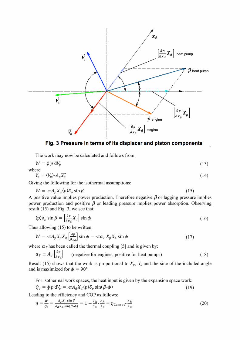
individually. So the combined effects of two or more stimuli are simply the added effects of the individual stimuli. This is why the compression volume variation is simply the added contributions of the piston and displacer motions. The pressure is treated similarly. Consider the displacer stationary and only the piston moving. It can be seen that there will be a pressure change in phase with the piston motions. Call this the piston pressure factor pp. For the displacer moving and the piston stationary, the pressure change will depend on the compression and expansion space temperatures. If the expansion space is warmer than the compression space, then positive displacer motions will result in decreasing pressure because the gas is moved to a cooler region for positive displacer motions. This is denoted as the displacer pressure factor pd. If the temperatures are reversed, i.e., the expansion space is colder than the compression space, the pressure will increase for positive displacer motions. Clearly from Fig. 3, the resulting pressure will lead in the case of the expansion space being warmer than the compression space and lag in the vice versa case. This is of course the difference in pressure phase for a power producing device and a heat lifting device.

From the foregoing, the pressure variations may therefore be written:

! ≈ ! + %&%'(

)& + %&%'*

)+ (3)

where !" ≝ $"

$%& and (4)

!" ≝ $%$&'

(5) There are many ways to determine pp and pd, including experimental measurement. For

simplicity, we will follow the isothermal assumptions of Schmidt [4] to derive the pressure in terms of xd and xp. The details being elementary, are excluded:

! = ! ##$%& '(,'+

≈ ! 1 − /& 0&, 01 (6)

where !" #", #% = '

()- '(+ ,%- -.()

/01 -

-2()

/21 (7)

and ! = #$

%&+ #&

%&+ () *+ %, %&

%,-%&+ #,

%,+ #.

%, (8)

Giving: !"!#$

≈ "&'$()

(9) !"!#$

≈ - "'

()*- ()+ ,-- ./)* (10)

And, finally the pressure in phasor form:

" = " + " ≈ " 1 + '(∠* (11) where

!"∠$ = &'

&()- &(+ ,-- ./() 0-∠1-

.2()0" (12)

The work may now be calculated and follows from:! = #d&' (13)

where !" = !" -%"&" (14)

Giving the following for the isothermal assumptions:

! = -$%&'& ( )& sin - (15) A positive value implies power production. Therefore negative β or lagging pressure implies power production and positive β or leading pressure implies power absorption. Observing result (15) and Fig. 3, we see that:

! "# sin ' = )#)*+

,- sin. (16)

Thus allowing (15) to be written:

! = -$%&'&'( )&)*+

sin/ = -$01 '&'( sin/ (17)

where α T has been called the thermal coupling [5] and is given by: !" ≡ $% &%

&'( (negative for engines, positive for heat pumps) (18)

Result (15) shows that the work is proportional to Xp, Xd and the sine of the included angle and is maximized for ! = 90°.

For isothermal work spaces, the heat input is given by the expansion space work: !" = $ d&" = -()*+* $ ,- sin 1-2 (19)

Leading to the efficiency and COP as follows:

! = #$%= &'(' )*+ ,

&-(- )*+ ,-/ = 1 − 2324- &5&- = !678+9:- &5&- (20)

COP = %&'()*+,-

./0102%&'()*+,- (21)

The reduction of the Carnot performance due to the area ratio reflects the fact that the rod area, AR is needed to provide non-recoverable work to the displacer to overcome flow losses. The maximum work condition ! = 90°, does not necessarily imply maximum efficiency.

We now turn our attention to the mass flows which are important in the evaluation of flow

losses and heat transfer. By our convention, positive mass flow at the compression space / rejecter boundary is the negative value of the rate of change of the mass within the compression space. For the isothermal system or where temperature variations are small compared to volume and pressure variations, the compression space boundary mass flow may be written:

!" = -%" = - &'()*,"+ ./

)*0 (22)

Increasing mass in the expansion space results in positive expansion space boundary mass flow, therefore:

!" = %" = &'

()*+"+ -.

)*/ (23)

Noting that the first derivative of a phasor is in quadrature (90°) to the original phasor, it is

possible to construct the phasors for the boundary mass flows from (22) and (23). Fig. 4 shows this for engines and Fig. 5 for heat pumps. Any mass flow within the machine will fall on a line connecting !" to !" as indicated by !" in Fig. 4.

Regenerator heat transfer is made up of the enthalpy entering its two ends and the change

of internal energy due to the expansion and compression of the gas within the regenerator. The rate equation representing these processes is as follows:

!" = $% &'( ) + $+ ,-."--,0.0" (24)

The regenerator boundary mass flows need to include the effect of mass change within the associated heat exchanger. These results are:

!"# = - &'()*,-+ /0 1/*

)*2 (25)

"#$ = &'

()*+,+ ./ 0.*

)*1 (26)

There is now sufficient information to plot the regenerator heat transfer phasor as shown in Fig. 6 for engines and Fig 7 for heat pumps. Note that the regenerator heat transfer is not necessarily in quadrature with the displacer motion. Also note that for engines, the regenerator heat transfer is almost in phase with regenerator mass flow. That is, the gas is heated as it flows towards the expansion space. For heat pumps, the heat transfer is almost opposite to the mass flow, as would be expected. Furthermore, regenerator heat transfer is ideally imagined as a constant volume process implying maximum heat transfer at minimum volume change. For that to happen, regenerator heat transfer should be roughly in phase or anti-phase with total volume variations. From Figs. 6 and 7 one can see that regenerator heat transfer has this approximate relationship with !" .

The unidirectional regenerator heat transferred is simply: !" = $

% !"d' = (% !")*+

) (ϕ is zero crossing point and phase) (27)

The regenerator effectiveness may now be defined [6]. ! = #$_&'( #$ (28)

The unregenerated energy must be accounted for by external heat transfer. Therefore: !"_$%& = !( + !* 1 − - (29)

From which the following results are obtained for efficiency and COP:

!"#$ = &'()*)+ ',-

= &./0123-56 57'( ',- 8* 8+

(30)

COP$%& = COP 1 − *+*,

1 − - = ./012345678./01234569: 9;

1 − *+*,

1 − - (31)

Where both the lost work due to driving the displacer and the effects of imperfect regeneration have been accounted for. The heat transfer ratio !" !# is a critical parameter and ranges from about 4 for engines to about 200 for cryocoolers. The area ratio !" !# generally ranges roughly between 0.05 to around 0.15. For example, the well described RE-1000 machine [7] has an area ratio of 0.085 and a heat transfer ratio of about 4. 3. MECHANICAL DYNAMICS

The phasor description of the thermodynamic processes extends directly to the mechanical

dynamics. Referring to Fig. 1, the force balance of the displacer is as follows: !"#" = %"-%' ()-%"(*-+"_-./0 #"-#) (32)

The bounce space pressure swing is assumed to be small compared to the working space and has therefore been neglected. Further, noting that (pc - pe) is simply the pressure drop across the heat exchanger loop, Δp, (32) becomes:

!"#" = %"Δ'-%)'*-+"_-./0 #"-#* (33) The Δp term is the result of flow dissipation in the heat exchangers. Since this is a dissipative force, it may be represented as a function of displacer, piston and casing velocities (! terms). The pc term is taken as a function of displacer, piston and casing displacements (x terms). We will furthermore assume a perfectly balanced machine (xc = 0). Equation (33) may therefore be written:

!"#" + %"#"+%"'#' + ("#"+)'#' = 0 (34) where

!" ≡ -%" &'(&)*

(35)

!"# ≡ -&" '(#')*

(piston gas flow coupling, typically negative) (36)

!" ≡ !"_%&'( + *+ ,-.,/0

(37)

!" ≡ $% &"'&()

(piston pressure coupling) (38)

Some researchers [8] prefer to combine the pressure terms into a single term called the displacer rod force, which is in phase with the pressure, as follows:

!" = $% &'(&)*

+" + &'(&)-

+' (39)

Again, noting that the first derivative rotates the phasor by 90° and the second derivative by 180°, equation (34) may be represented in phasor form as shown in Figs. 8 and 9. In the case of an engine, the change of pressure with displacer motion is negative so Kd is reduced by the !" #$%

#&' term whereas for a heat pump, this term will add to the spring effect. We also

have the direction and magnitude of the pressure drop, so the expansion space pressure may be added to the phasor diagram.

The piston equation follows similarly and is also shown in Figs. 8 and 9.

!"#" + %"#"+'(#) + '*+ = 0 (40) where α T is the thermal coupling as in (18), !"# is the current force due to the linear alternator or motor and has the phase of the current, and

!" ≡ $" %"&%'(

(41)

For perfect balance (xc = 0) the balance mass phasor must satisfy the system momentum equation.

!"#" + !%#% + !&#& = 0 (42) This happens when the balance mass is resonant at the operating frequency.

The last items to add to the mechanical dynamics phasor diagram are the voltages for the

motor / alternator, also called a linear force transducer. The applied voltage is as follows: !"## = !%&'-!)-!*"+ (alternator) !"## = !%&' + !) + !*"+ (motor) (43)

where Vind is the voltage generated by the movement of the magnets and is always in phase with piston velocity, and VL and VRac are given by:

!" = $& (inductive voltage) (44) !"#$ = &'(* (voltage drop across effective resistance at ω ) (45)

The current in the linear alternator / motor may also be determined from the mechanical dynamics phasor diagrams. From Figs. 8 and 9 we see that:

!"# sin'( = !* +, sin- (46) giving:

! = #$#%&' ()* +

()* ,- (47)

The current phase may be obtained from the geometry of the piston force diagram.

!" = tan-( )* +, -./ 0)* +, 12- 0345+5-6578+5

(48)

The alternator / motor efficiency is given by accounting for the energy dissipated in Rac.

!" = 1 − 2' ()*+,-. (49)

This result is only approximately true for motors but the error is not large when the efficiency is better than 85%. For alternators it is accurate.

4. DISCUSSION AND CONCLUSIONS

The principle of superposition allows the phasor description to offer insights that are not

obvious from the classical analyses. The relationship between processes is easier to understand and more importantly, the descriptive language that can be applied by this method is succinct and precise. The consequences of the non-ideal processes associated with flow losses, imperfect regeneration and transducer efficiency are easily included. Of course, the phasor description assumes that the processes can be modeled by first harmonic or sinusoidal functions. This is only true for a linear system which is generally a good approximation for free-piston machines [9]. For crank machines, this may not be a valid model since the mechanical motions often have significant higher harmonics, which together with the higher harmonics in the gas processes, will result in additional terms of significance. As a general rule, if the mechanical motions of the piston and displacer are closely sinusoidal, the system may be linearized without too much penalty to accuracy.

REFERENCES [1] G. T. Reader and C. Hooper, Stirling Engines, London: E. & F. N. Spon, 1983. [2] F. A. Creswick, “Thermal Design of Stirling Cycle Machines,” in International

Automotive Engineering Congress, Detroit, 1965. [3] I. Urieli, “A Computer Simulation of Stirling Cycle Machines,” University of the

Witwatersrand, Johannesburg, 1977. [4] G. Schmidt, “Theory der Lehmann'schen calorischen machine,” Zeitschrift des Vereines

Deutscher Ingenieure, vol. 15, pp. 1-12, part 1. 97-112, part 2, Jan. - Feb. 1871. [5] R. W. Redlich and D. M. Berchowitz, “Linear Dynamics of Free-Piston Stirling Engines,”

Proc Instn Mech Engrs, vol. 199, no. A3, pp. 203-213, March 1985. [6] I. Urieli and D. M. Berchowitz, Stirling Cycle Engine Analysis, Bristol: Adam Hilger,

1984. [7] J. Schreiber, “Testing and Performance Characteristics of a 1kW Free-Piston Stirling

Engine,” NASA-Lewis, Cleveland, 1983. [8] J. G. Wood, “A program for Predicting the Dynamics of Free-Piston Stirling Engines,”

1980. [9] D. M. Berchowitz, “Free-Piston Stirling Coolers,” in International Refrigeration

Conference - Energy Efficiency and New Refrigerants, 1992.

NOMENCLATURE A = area (m2) COP = coefficient of performance D = damping coefficient (Ns/m) Ddp = displacer – piston damping coefft. (Ns/m) I = current (A) K = effective spring stiffness (N/m) Kd_mech = displacer mechanical spring (N/m) L = inductance (H) m = mass (kg) p = pressure (Pa), pressure factor (Pa/m)

α = volume phase angle (°) α l = linear alternator / motor constant (N/A) α p = pressure coupling (N/m) α Τ = thermal coupling (N/m) β = pressure phase (°) δp = pressure ratio (-)

Subscripts a = accepter b = balance mass c = compression space, casing d = displacer e = expansion space

Other = first derivative w.r.t. time = second derivative w.r.t. time

Q = heat input (J) R = gas constant (J/kg K) Rac = effective resistance (Ω) S = collection of terms (m3/K) T = temperature (K) V = volume (m3), voltage (V) w = mass flow (kg/s) W = work (J) x = displacement (m) X = amplitude (m)

ε = regenerator effectiveness (-) φ = displacer phase (°) η = efficiency (-) ϕ I = current phase (°) ω = frequency (rads/s)

k = rejecter l = linear alternator / motor p = piston r = regenerator R = displacer drive

= mean value = phasor quantity when ambiguous