a primer: logit models for social networks

Ž .Social Networks 21 1999 37–66

A pU primer: logit models for social networks

Carolyn J. Anderson a,b,), Stanley Wasserman b,c,d,1,Bradley Crouch b,2

a Department of Educational Psychology, UniÕersity of Illinois, Champaign, USAb Department of Psychology, UniÕersity of Illinois, Champaign, USA

c Department of Statistics, UniÕersity of Illinois, Champaign, USAd The Beckman Institute for AdÕanced Science and Technology, UniÕersity of Illinois, Champaign, USA

Abstract

A major criticism of the statistical models for analyzing social networks developed by Holland, Leinhardt,wand others Holland, P.W., Leinhardt, S., 1977. Notes on the statistical analysis of social network data;

Holland, P.W., Leinhardt, S., 1981. An exponential family of probability distributions for directed graphs.Ž .Journal of the American Statistical Association. 76, pp. 33–65 with discussion ; Fienberg, S.E., Wasserman,

Ž .S., 1981. Categorical data analysis of single sociometric relations. In: Leinhardt, S. Ed. , SociologicalMethodology 1981, San Francisco: Jossey-Bass, pp. 156–192; Fienberg, S.E., Meyer, M.M., Wasserman, S.,1985. Statistical analysis of multiple sociometric relations. Journal of the American Statistical Association, 80,pp. 51–67; Wasserman, S., Weaver, S., 1985. Statistical analysis of binary relational data: Parameterestimation. Journal of Mathematical Psychology. 29, pp. 406–427; Wasserman, S., 1987. Conformity of two

xsociometric relations. Psychometrika. 52, pp. 3–18 is the very strong independence assumption made oninteracting individuals or units within a network or group. This limiting assumption is no longer necessary

wgiven recent developments on models for random graphs made by Frank and Strauss Frank, O., Strauss, D.,x1986. Markov graphs. Journal of the American Statistical Association. 81, pp. 832–842 and Strauss and Ikeda

wStrauss, D., Ikeda, M., 1990. Pseudolikelihood estimation for social networks. Journal of the AmericanxStatistical Association. 85, pp. 204–212 . The resulting models are extremely flexible and easy to fit to data.

wAlthough Wasserman and Pattison Wasserman, S., Pattison, P., 1996. Logit models and logistic regressionsU xfor social networks: I. An introduction to Markov random graphs and p . Psychometrika. 60, pp. 401–426

present a derivation and extension of these models, this paper is a primer on how to use these importantŽ .breakthroughs to model the relationships between actors individuals, units within a single network and

provides an extension of the models to multiple networks. The models for multiple networks permitresearchers to study how groups are similar andror how they are different. The models for single and multiple

) Corresponding author. Department of Educational Psychology, University of Illinois, 230 Education Bldg.,1310 South Sixth St., Champaign, IL 61820-6990, USA. Tel.: q1-217-333-2245; Fax: q1-217-244-7620;E-mail: [email protected]

1 E-mail: [email protected] E-mail: [email protected]

0378-8733r99r$ - see front matter q 1999 Elsevier Science B.V. All rights reserved.Ž .PII: S0378-8733 98 00012-4

( )C.J. Anderson et al.rSocial Networks 21 1999 37–6638

networks and the modeling process are illustrated using friendship data from elementary school children fromwa study by Parker and Asher Parker, J.G., Asher, S.R., 1993. Friendship and friendship quality in middle

childhood: Links with peer group acceptance and feelings of loneliness and social dissatisfaction. Developmen-xtal Psychology. 29, pp. 611–621 . q 1999 Elsevier Science B.V. All rights reserved.

Social network analysis has been used for more than sixty years to advancesubstantive research in the social and behavioral sciences. The disciplines that haveutilized the social network paradigm include anthropology, communications, marketing,political science, organizational studies, as well as much of sociology, and community,clinical, and social psychology. The range of applications of social network methodol-ogy has grown enormously since major methodological breakthroughs of the 1970’s and1980’s.

The explosion of network research since the early 1970’s focuses primarily on socialnetworks in modern societies, whether the societies be small groups or nation-states. Thesocial network perspective has most likely grown in popularity because it enables

Ž .researchers to model the social relationships among interacting units or social actorsand the implications of their patterns. Many researchers have found that the networkperspective allows new leverage for answering standard social and behavioral scienceresearch questions by giving precise formal definitions to aspects of the behavioral,

Ž .political, economic, or social structural environment Wasserman and Faust, 1994 .The structural environment can be expressed as patterns or regularities in relation-

Žships among interacting units Wasserman and Faust, 1994; Wellman and Wasserman,.1998 . It is common to refer to the presence of regular patterns in relationships simply as

structure. Social network analysis is designed to model these patterns. Researchersdeveloped methods to test specific hypotheses about network structural properties

Žarising in the course of substantive research and model testing see the edited volumesof Wasserman and Galaskiewicz, 1994; Wellman and Berkowitz, 1997a; or the papersby Wellman, 1983; Wellman et al., 1997; Wellman and Berkowitz, 1997b, for exam-

.ples . In turn, the methodology has allowed us and other behavioral researchers to dobetter research; for example, we can now more effectively model social support

Ž .networks Walker et al., 1993; Walker, 1995 , interorganizational corporate relationshipsŽ . ŽGalaskiewicz and Wasserman, 1989, 1990 , cognitive psychological structures Krack-

.hardt, 1987; Pattison, 1994; Kumbasar et al., 1994; Koehly, 1996 and intragroupŽ .decision-making processes Arrow, 1994, 1997; see also Robins et al., 1995 . The result

of this symbiotic relationship between theory and method provides a strong groundingfor the application of network analytic techniques.

One very important area of research is the development of predictive models forrelational variables. This methodology allows a researcher to easily model the relation-ship between a specific social relation, measured on pairs of actors taken from some setof actors, and a specific collection of explanatory variables. Three aspects of themeasurements of these variables makes this a particularly tricky problem. First, the

Žresponse variable is usually dichotomous and almost always discrete for example, actor.i does or does not have a relational tie to actor j ; secondly, the nature of social relations

imposes specific associations among the realizations of the response and explanatory

( )C.J. Anderson et al.rSocial Networks 21 1999 37–66 39

Žvariables such as the strong association between actor i’s relational tie to actor j, and.actor j’s relational tie to actor i . Lastly, the explanatory variables can be of several

Ž .different types. The work of Wasserman and Pattison 1996 and Pattison and Wasser-Ž .man 1998 , described below, provides a new step in answering these problems by their

Ž .elaboration on a class of models first proposed by Frank and Strauss 1986 . AlsoŽ . Ž .relevant to this work is Frank 1991 and Frank and Nowicki 1993 .

Ž .After describing a data set taken from Parker and Asher 1993 , a study of friendshipand acceptance of third- through fifth-grade children, we present the notation that we useto describe mathematically this new family of models, which has been labeled pU. Weintroduce pU , and give an introduction to logit models and logistic regressions to allowreaders to appreciate the nature and generality of this approach to social network

Žanalysis. We provide a brief overview of the statistical theory for these models much.more detail can be found in the references mentioned below and a detailed guide to

fitting and evaluating the logit version of pU. All these new ideas are demonstratedusing the Parker and Asher classroom data using pU directly, as well as a generalizationof pU to multiple networks.

1. Some history

ŽHighlights of social network research described in detail in Wasserman and Faust,.1994 are many. These include the triadic analyses of Davis, Leinhardt, and Holland

ŽDavis, 1967, 1970, 1979; Davis and Leinhardt, 1972; Holland and Leinhardt, 1970,.1971, 1972, 1975, 1978, 1979; Leinhardt, 1972, 1973 designed to study structural

balance and transitivity theory, and the blockmodel methods and algebraic approaches ofŽWhite, Boorman, Breiger, and Arabie Breiger et al., 1975; White et al., 1976; Boorman

and White, 1976; White, 1977; Arabie et al., 1978; Arabie and Boorman, 1982; Arabie.and Hubert, 1992; Pattison, 1993 , implementing the very important notion of structural

Ž .equivalence of Lorrain and White 1971 . In addition, the basic statistical models ofŽHolland, Leinhardt, and others Holland and Leinhardt, 1977, 1981; Fienberg and

Wasserman, 1981; Fienberg et al., 1985; Wasserman and Weaver, 1985; Wang and.Wong, 1987; Wasserman, 1987 , particularly p , are of importance.1

ŽResearch in the 1980’s helped refine the statistical models of the 1970’s see for.example, Wasserman, 1987; Wasserman and Iacobucci, 1988 , but the nature of the

models is quite limiting—severe independence assumptions are imposed on the mea-sured variables. The pU family of models we will describe here, developed by

Ž . Ž . ŽWasserman and Pattison 1996 and Pattison and Wasserman 1998 see also Rennolls,. Ž .1995 based on the pathbreaking models for random graphs of Frank and Strauss 1986

Ž .and Strauss and Ikeda 1990 , however, makes no such assumption. The formulationŽ .presented by Wasserman and Pattison 1996 allows these models to be viewed in a very

standard responserexplanatory variables setting in which the response variable is a logit,or log odds of the probability that a relational tie is present, and in which theexplanatory variables can be quite general. Further, the pU family is easily fit approxi-mately using standard logistic regression modeling software.


These models postulate a very general dependence structure for the elements of thenetwork, and are sufficiently general that, as a class, they contain all possible distribu-tions for networks of a given size. The Markov graphs first described by Frank andStrauss are generalizations of Markov random fields designed for spatial interaction dataŽStrauss, 1977; Wasserman, 1978; Speed, 1978; Kindermann and Snell, 1980; Ripley,

.1981 and are based on the well-known model named after the German physicist IsingŽ .see p. 51 of Ising, 1925; see also Preston, 1974; Griffeath, 1979 .

As mentioned, the pU family first arose in spatial modeling. A very generalŽ .formulation of it, presented by Wasserman and Pattison 1996 , proceeds by considering

a family of binary variables, perhaps recording whether or not a collection of objectsŽ .arrayed in two-dimensional space such as plants in a field have a specific dichotomous

Ž . Ž .property such as a disease . As described in such texts as Ripley 1981 and CressieŽ .1991 , one can write the model as an autologistic regression model, in which the logodds of the probability that one of the objects has the property, is regressed linearly onfunctions of the other variables.

These autologistic models arise in many different situations. A nice review of theirŽ . Ž .variety is given by Strauss 1992 . Geyer and Thompson 1992 give a detailed history

of statistical methods for these autologistic models, which usually incorporate rathercomplicated dependencies among the variables.

Ž .Pattison and Wasserman 1998 used an alternative approach to arrive at the samegeneral class of models. Their derivation is based on the Hammersley–Clifford TheoremŽ .discussed by Besag, 1974, and used by Frank and Strauss, 1986 . When applied to a

Ž .graph representing, say, a social network , the theorem yields a characterization of theprobability distribution for a random graph. The distinctions between the two approaches

Ž .are nicely described by Diggle 1996 . Here, we will work with the autologisticregression approach, because of its ease of presentation.

2. Examples

Ž .Parker and Asher 1993 conducted a study to investigate the relationship betweenŽ .elementary school children’s friendships and peer group classroom acceptance. As part

Žof the study, Parker and Asher collected network data for children in 36 classrooms 12.third-grade, 10 fourth-grade, and 14 fifth-grade from five public elementary schools in

a midwestern US community. There were a total of 881 children. We use part of thisdata set to illustrate the methods described here.

Each child in each class was given a roster of the children in hisrher class and wastold to choose hisrher ‘very best friend’, three ‘best friends’, and an unlimited number

Ž .of ‘friends’. Thus, Parker and Asher gathered data on 36 networks classrooms , withŽ .three relations very best friendship, best friendship, friendship measured for each

Žnetwork. Additional data were collected on the children attribute information on these. Žsocial actors including gender, age, race, loneliness using the self-report questionnaire

. Žof Asher and Wheeler, 1985, adapted from Asher et al., 1984 , and acceptance based onhow much classmates liked to play with each classmate, using a ‘roster-and-rating’

.network procedure .


ŽParker and Asher focus much of their attention on mutual friendship relations actor i.and actor j both choose each other as friends , and study the differences between

children with respect to acceptance and friendship quality. We have chosen three of the36 classrooms to illustrate pU ; the three classrooms, one from each grade, will be

Žanalyzed individually as well as simultaneously so that we can characterize differences.among the classes . Given Parker and Asher’s emphasis on friendship, we fit models to

Žthese three classrooms that emphasize dyadic effects as opposed to transitive or.higher-level effects , especially choices made by and received by children and whether

these choices were reciprocal or mutual. In addition, to keep our analyses simple, weignore the distinctions among the quality or strength of the reported friendships andcreate one relation reflecting friendship. This relation is not necessarily ‘symmetric’—ican choose j, but j need not choose i as a friend—so that we can model mutualityeffects. Although valued relations with several defined strengths can be modeled directlyŽ .see Wasserman and Faust, 1994, chapter 15; and especially, Robins et al., 1998 , here

Fig. 1. The directed graph of the fifth-grade classroom where the squares and circles respectively represent theboys and girls, and the arrows depict the presence of a directed friendship relational tie.


we have chosen to combine the three dichotomous friendship relations into a single, alsodichotomous, relation; thus, if i says that j is either a ‘very best friend’, ‘best friend’, orsimply ‘friend’, we will code a ‘friendship’ relational tie as being present. A graphicalrepresentation of this friendship relation is shown in Fig. 1, where the squares andcircles respectively represent the boys and girls in the fifth-grade classroom and thearrows depict the presence of a directed friendship relational tie.

Our analyses of this basic relation will include several important actor attributemeasurements that we hypothesize have an association with friendship. These factors,

Ž .identified by many including Parker and Asher as influencing a child’s participation infriendships, include gender, age, and classroom membership; therefore, we incorporatethese factors into our pU models of the friendship relation.

U Ž .The first exposition of p was for single networks Wasserman and Pattison, 1996 ,which for the data here allows us to study each classroom individually. To studysimilarities and differences simultaneously across the classrooms, we develop the firstpU-type models for multiple networks.

3. Some notation

A social relation is defined on a set of g social actors or individuals, and measuresŽ .how these actors are related to or tied to or linked to each other. We let NN denote a

Table 1Third-grade classroom—friendship relation

Child Boys Girls

1 2 3 4 5 11 7 8 20 10 16 19 13 21 15 12 17 18 14 9 6 22

Boys 1 1 1 12 1 1 1 1 1 1 1 1 1 1 1 13 1 1 14 1 1 1 1 15 1 1 1 1 1 1 1 1 1 1 1 1

11 1 1 1 1 1 1 1 1 1 17 1 1 1 1 1 1 1 1 18 1 1 1 1 1 1 1 1 1 1 1 1

20 1 1 1 1 1 1 1 1 1 1 1 110 1 1 1 1 1 116 1 1 1 1 1 1 1 1 119 1 1 1 1 1 1 1 1 1 1 1 1 113 1 1 1 1 121 1 1 1 1 1 1 1

Girls 15 1 1 1 1 1 1 112 1 1 1 1 1 1 1 1 1 1 1 1 1 1 1 1 117 1 1 1 118 1 1 114 1 1 1 1 1 1 1 1 19 1 1 1 1 1 16 1 1 1 1

22 1 1 1 1 1 1 1 1 1


� 4set of actors: NNs 1, 2, PPP , g . A dichotomous social relation, XX , is a set of orderedpairs of actors such that the first actor in the pair has a relational tie to the second actorin the pair; we can write i™ j. The main statistical focus in the literature and here as

Ž .well, has been on models for single or univariate , dichotomous, directed relationsŽ .represented as directed graphs .

Ž .Such a social relation can be represented by a g=g sociomatrix, X, where the i, jŽ .entry in the matrix which we denote by X is the value of the tie from actor i to actori j

j on that relation. For a dichotomous relation,

1 if i™ jX si j ½0 otherwise.

We will assume here that these quantities are random variables.The sociomatrices for the three Parker and Asher classrooms that we analyze here are

shown in Tables 1–3. These three were chosen at random from the larger set ofclassrooms; each represents a different grade. We have ‘suppressed’ the zeros in thesetables to make the sociomatrices easier to examine, and we have permuted the rows andcolumns of these arrays to place the boys and girls together. Note the strong gender

Table 2Fourth-grade classroom—friendship relation

Child Boys Girls

1 14 6 4 17 12 13 8 18 10 11 22 20 3 9 7 5 15 19 2 21 16 23 24

Boys 1 1 1 1 1 114 1 1 1 1 1 16 1 1 1 1 1 14 1 1 1 1 1 1

17 1 1 1 1 1 112 1 1 1 1 1 1 1 113 1 1 1 1 1 18 1 1 1 1 1 1 1 1

18 1 1 1 1 1 110 1 1 1 1 1 111 1 1 1 1 1 1 1 1 1 1 1 1 1 1 122 1 1 1 120 1 1 1 1 1 1 1 1

Girls 3 1 1 1 1 1 1 1 19 1 1 1 1 1 1 1 1 1 1 17 1 1 1 1 1 1 15 1 1 1 1 1

15 1 1 119 1 1 1 1 1 12 1 1 1 1 1 1 1

21 1 1 1 1 1 1 1 1 116 1 1 1 1 1 1 1 123 1 1 124 1 1 1 1


Table 3Fifth-grade classroom—friendship relation

Child Boys Girls

1 2 14 15 5 17 18 19 9 10 11 12 16 13 4 3 6 7 8 20 21 22

Boys 1 1 1 1 1 1 1 12 1 1 1 1 1 1

14 1 1 1 1 1 1 1 1 1 115 1 1 1 1 1 1 15 1 1 1 1 1 1 1

17 1 1 1 1 1 1 1 1 118 1 1 1 119 1 1 1 19 1 1 1

10 1 1 111 1 1 112 1 1 1 1 1 1 116 1 1 1

Girls 13 1 1 1 14 1 1 1 1 13 1 16 17 18 1 1 1

20 1 1 1 1 1 1 121 1 1 122 1 1 1 1

effects—there are relatively few friendships across genders. One would certainly wantto model these data using gender as an explanatory variable.

One can calculate many graph-theoretic characteristics about the relation from thesociomatrix X. Examples of various characteristics are numerous, and include the

Ž .number of ties, L, the number of mutual dyads or reciprocated ties , M, and theg Žoutdegree of the ith actor, X sÝ X the number of relational ties originatingiq js1 i j

.with the i actor . A very wide range of such statistics can be found in Wasserman andŽ .Pattison 1996 . Descriptions of these characteristics can be found in Chapters 3 and 4 of

Ž .Wasserman and Faust 1994 . One can define actor-level quantities such as gender, age,grade, race, ethnicity, work-group, seniority, and so on. If one has measurements on

Ž .more than one set of actors such as with the Parker and Asher classrooms , one caneven code the classroom of each actor into a set of variables for a ‘multi-group’ socialnetwork analysis; extensions of the pU family to such data are described later.

To specify our new family of models, we need to create three other sociomatricesfrom X, so we need still more notation. From X, we define Xq as the sociomatrix fori j

the relation formed from XX where there is always a relational tie from i to j, Xy as thei j

sociomatrix for the relation formed from XX where there is never a relational tie from iŽ .to j or the tie is forced to be at level 0 . For example, for the friendship relation

measured on the third-graders, the sociomatrix Xq has an entry of 1 in the cell13


specifying whether child 1 has a tie to child 3, while the sociomatrix Xy has an entry of15

0 in the cell specifying whether child 1 has a tie to child 5. Lastly, we define X c as thei jc � Ž . Ž .4complement relation for the tie from i to j: X s X , with k, l / i, j . Thei j k l

complement relation has no relational tie coded from i to j—one can view this singlevariable as missing. Complement sociomatrices give all the relational information exceptfor the value of i’s tie to j.

4. An introduction to pU

4.1. pU

The family of models pU contains the Markov random graphs of Frank and StraussŽ .1986 as a special case, as well as the dyadic interaction model p of Holland and1

Ž . Ž .Leinhardt 1977 Holland and Leinhardt, 1981; Fienberg and Wasserman, 1981 . Webegin with a collection of explanatory variables, all functions of the observed data x,

Ž . Ž . Ž .that we denote by z x , z x , PPP , z x .1 2 rŽAny graph-theoretic characteristic of the relation for example, the number of

.relational ties or the number of reciprocated ties , or attribute measurement on the actorsŽ . Ž .for example, gender or age is a potential explanatory z x . The model parameters, thek

elements of the vector u , will be the coefficients of a linear function of theseexplanatory variables as in standard linear models:

u z x qu z x q PPP qu z x .Ž . Ž . Ž .1 1 2 2 r r

Ž .The response variable is the probability of the observed x, Pr Xsx ; but sinceprobabilities must be between 0 and 1, one usually models not the probability, but alogarithmic transformation of it. Thus, we postulate that

log Pr Xsx is proportional to u z x q PPP qu z x . 1Ž . Ž . Ž . Ž .1 1 r r

Ž .Now all that we must do is normalize the right side of 1 to turn this into a properŽ .probability model so that the sum of Pr Xsx over all possible directed graphs is

unity.From these concerns, comes the basic log linear model

exp u X z x exp u z x q PPP qu z x� 4 � 4Ž . Ž . Ž .1 1 r rPr Xsx s s 2Ž . Ž .

k u k uŽ . Ž .Ž .where u is a vector of the r model parameters, z x is the vector of the r explanatory

variables, and k is our normalizing constant that ensures that the probabilities sum toŽ .unity. Following the terminology of Wasserman and Pattison 1996 , we refer to models

Ž . Uof the form 2 as p .Ž .In Model 2 , the u parameters are the unknown ‘regression’ coefficients and must

Ž .be estimated. If we ignore the function k in the denominator of Model 2 , and takeŽ .logarithms of the left side as in 1 , we can see that the explanatory variables enter in a

standard, additive manner. We note that one might need constraints on the elements of uto ensure a set of uniquely-determined parameters, as is often the case in general andgeneralized linear models.


Table 4Some parameters and graph statistics for pU models

Ž .Type Parameter Graph statistic z xLabel

DyadicChoice f LsÝ X s Xi j i j qqMutuality r MsÝ X Xi- j i j ji

TriadicTransitivity t T sÝ X X XT T i , j ,k i j jk i k

Ž .Intransitivity t T sÝ X X 1y XI I i , j ,k i j jk i k

Cyclicity t T sÝ X X XC C i , j ,k i j jk k i

2-in-stars s S sÝ X XI I i , j ,k ji k i

2-out-stars s S sÝ X XO O i , j ,k i j i k

2-mixed-stars s S sÝ X XM M i , j ,k ji i k

r s r sSubgroup effects f B sÝ X di , j i j i j;r s

IndiÕidual leÕelŽ .Differential expansiveness a X soutdegree degree centralityi iqŽ .Differential attractiveness b X s indegree degree prestigei q i

The indicator quantity d s1 if i is in the r th subgroup and j is in the sth, and 0 otherwise.i j;r s

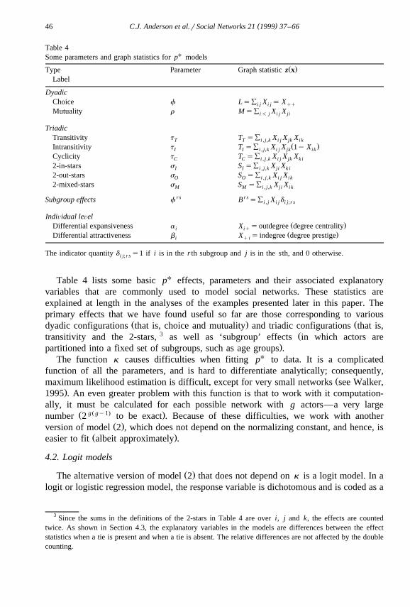
Table 4 lists some basic pU effects, parameters and their associated explanatoryvariables that are commonly used to model social networks. These statistics areexplained at length in the analyses of the examples presented later in this paper. Theprimary effects that we have found useful so far are those corresponding to various

Ž . Ždyadic configurations that is, choice and mutuality and triadic configurations that is,3 Žtransitivity and the 2-stars, as well as ‘subgroup’ effects in which actors are

.partitioned into a fixed set of subgroups, such as age groups .The function k causes difficulties when fitting pU to data. It is a complicated

function of all the parameters, and is hard to differentiate analytically; consequently,Žmaximum likelihood estimation is difficult, except for very small networks see Walker,

.1995 . An even greater problem with this function is that to work with it computation-ally, it must be calculated for each possible network with g actors—a very large

Ž g Ž gy1. .number 2 to be exact . Because of these difficulties, we work with anotherŽ .version of model 2 , which does not depend on the normalizing constant, and hence, is

Ž .easier to fit albeit approximately .

4.2. Logit models

Ž .The alternative version of model 2 that does not depend on k is a logit model. In alogit or logistic regression model, the response variable is dichotomous and is coded as a

3 Since the sums in the definitions of the 2-stars in Table 4 are over i, j and k, the effects are countedtwice. As shown in Section 4.3, the explanatory variables in the models are differences between the effectstatistics when a tie is present and when a tie is absent. The relative differences are not affected by the doublecounting.


Ž U .binary variable for example, Y s1 or 0 , which is often assumed to have a binomialdistribution. Given the nature of this response variable, it is natural to model probabili-

Ž U .ties, Pr Y s1 . Probabilities are modeled as a function of a linear combination or aŽlinear predictor of the explanatory variables for example, b qb y q PPP qb y ,0 1 1 r r

.where the Y ’s are explanatory variables and the b ’s are regression coefficients . SinceŽ .probabilities must be between 0 and 1 and the linear predictor can theoretically equal

any value between y` and q`, probabilities are transformed into logits beforeequating them to the linear predictor. A logit is the logarithm of the odds that an ‘event’

Ž U .occurs for example, Y s1 . Setting the transformed probabilities or logits equal to thelinear predictor gives us

Pr Y U s1Ž .Ulogit Y s log sb qb Y q . . . qb Y 3Ž . Ž .0 1 1 r rUž /Pr Y s0Ž .

Typically, logit models are fit to data using maximum likelihood estimation.ŽTo interpret the parameters, the most natural way uses odds and odds ratios see

. Ž .Agresti, 1996, for other interpretations . Taking the exponential of 3 gives us amultiplicative model for the odds of the binary response variable; that is,

Pr Y U s1Ž .b b Y b Y0 1 1 r rsexp b qb Y q . . . qb Y se e . . . eŽ .0 1 1 r rUPr Y s0Ž .

Thus, the odds that an event occurs changes multiplicatively with changes in theexplanatory variables. For example, holding all variables except Y constant, the oddsk

U Ž . bkthat Y s1 when the explanatory variable Y s yq1 is e times the odds whenk

Y sy. In other words, the ratio of the odds or odds ratio for a one unit increase in Yk k

equals e bk.

4.3. Logit pU

The approach we take to simplify the pU family of models so that model parametersŽ .can be estimated was first described by Strauss and Ikeda 1990 . We use the fact that

the basic random variable, X , reflecting the presence or absence of a relational tie fromi j

i to j, is dichotomous. Hence, we can consider the odds that this tie is present—the ratioŽ . Ž .of Pr X s1 to Pr X s0 .i j i j

To recognize the fact that pU is a model not for the probabilities of individual ties,but for the entire collection of ties, we work not with these ‘marginal’ probabilities butwith probabilities conditional on all the other relational ties in the network. The

Ž .Hammersley–Clifford Theorem Besag, 1972, 1974, 1977 allows us to obtain theprobability of the entire network, the response function in our basic model, from theconditional probabilities. Further, the conditional probabilities allow us to use theobserved values of all ties as possible explanatory variables. Thus, we define theconditional odds as

< cPr X s1 XŽ .i j i j� 4exp v s , 4Ž .i j c<Pr X s0 XŽ .i j i j


Žwhere we statistically condition our probabilities on the complement relation defined.earlier which contains all the other ties in the network.

This approach has the advantage of yielding a model not dependent on the normaliz-Ž . Uing constant. The odds defined in 4 simplifies p substantially. Using the two other

relations defined earlier, Xq, formed from XX where the tie from i to j is forced to bei j

present, and Xy, where the tie from i to j is forced to be absent, we have:i j

< c X qPr X s1 X exp u z x� 4Ž .Ž .i j i j i j X q ys sexp u z x yz x . 5Ž .Ž . Ž .½ 5i j i jXc y<Pr X s0 X exp u z xŽ . � 4Ž .i j i j i j

From this result, we obtain the logit version of pU by taking the logarithm of the odds:

< cPr X s1 XŽ .i j i j X q yv s log su z x yz x . 6Ž .Ž . Ž .i j i j i jc½ 5<Pr X s0 XŽ .i j i j

Ž . w Ž q. Ž y.x Ž .If we define d z s z x yz x , then the logit Model 6 simplifies succinctly toi j i j i jX Ž .v su d z .i j i j

Ž .The expression d z is the collection of explanatory variables used to fit the logiti jU Ž .version of p . The elements of d z are changes in the measurements on the originali j

network explanatory variables that arise when x changes from 1 to 0. One takes the seti jŽ .of explanatory variables z x , and records the values of the statistics when x s1 andi j

Ž .when x s0. The differences in the statistics are the elements of d z . This version ofij i j

the model, in which a log odds is equated to a linear function of the components ofŽ . Ud z , will be referred to as the logit p family of models.i j

These models can include actor-attribute explanatory variables, such as the gender ofthe actors. We can allow model parameters to depend on the attributes; for example, wecan study the effect of the gender of the actors on tendencies toward mutuality ortransitivities.

The simplest way to use such actor-attributes as explanatory variables is to allow theU Ž .basic choice parameters of p the f parameters to depend on the values of the

Ž .attributes. So, for example, we might include the explanatory variable age of sender =Ž . Ž . Ž .the number of ties in the network , which is equivalent to y i Ý x , where y i is thek l k l

age of actor i. The parameter corresponding to this variable, f , would then reflect theage

effect of the age of the sending actor on the probability of the network. One could alsouse as an explanatory variable the age of the receiving actor, by including the

Ž . Ž .explanatory variable age of receiver = the number of ties in the network . Or, one� r s4could categorize the actors into age subgroups, and use a set of effects f , where

actor i is in age-subgroup r and actor j is in age-subgroup s.

4.4. Fitting and eÕaluating logit pU

Fitting pU to single networks or multiple networks is easy, provided one adopts not amaximum likelihood estimation of the model parameters but rather a pseudo-likelihoodestimation strategy that assumes that the logits v of the conditional probabilitiesi j

Ž .defined in Eq. 6 are statistically independent. Details of this strategy, first proposed by


Ž . Ž .Strauss 1986 and Strauss and Ikeda 1990 , can be found in Wasserman and PattisonŽ .1997 .

Maximizing this pseudo-likelihood function is equivalent to fitting a logistic regres-� 4sion model to the logits v . One takes the network data and the relevant actori j

attributes, and creates a vector of measurements on the response variable and a matrix ofŽ .measurements on the explanatory variables note that there is no intercept in the model .

These quantities are then ‘fed into’ a logistic regression computing package to getŽ . Umaximum pseudo-likelihood MPL estimates of the postulated p model parameters

and approximate standard errors. The example given below will illustrate this facility indetail.

To assess the statistical importance of a particular variable, one can fit two models:Žone with the variable and another without it while the other variables must remain the

. Ž 2 .same . The difference in pseudo-likelihood ratio statistics G can be evaluatedPL

approximately by referring the value to a x 2 distribution with degrees of freedom equalŽto the number of parameters associated with the variable in question Wasserman and

.Pattison, 1997; Pattison and Wasserman, 1998 .In addition to G2 , one can also examine the ratios of parameter estimates or linearPL

functions of parameter estimates, to their approximate standard errors. 4 The square ofŽ .such ratios are known as Wald statistics Agresti, 1990 and labeled here as Wald forPL

our pseudo-likelihood estimated parameters. Since both the parameter estimates and theestimates of the standard errors are maximum pseudo-likelihood estimates, Wald isPL

evaluated approximately by comparing it to the appropriate x 2 distribution.

5. Example: a single class

In this section, application of logit pU is illustrated for a single network by analyzingone class from the Parker and Asher data set. When analyzing a single network,individual-level parameters can be included in the model, as well as group-level orhomogeneous structural parameters. In a later section, all three classes are modeledsimultaneously to illustrate how generalizations of logit pU can be used to investigatewhether and how separate networks for the individual classes differ. Our multi-groupmodels include only group-level explanatory variables; however, attribute informationregarding individual children can be included in the models. 5

The process by which we select a model for a data set is demonstrated by analyzingŽ .the fourth-grade class Table 2 . The first step in the modeling process is the identifica-

Ž .tion of the effects or variables that are potentially important and interesting . The modelwith all of these effects is the most complex model that is fit and is our initial model.The next step is to fit simpler, more restrictive models until no simpler model can be

4 Just as the parameter estimates are maximum pseudo-likelihood estimates, so too are the estimatedstandard errors of the parameter estimates.

5 Data files and SAS programs used to perform the analyses described here are available electronically atthe internet address s.psych.uiuc.edu, in the pubrwassermanrpstarrprimer subdirectory, or at the URLhttp:rrkentucky.psych.uiuc.edurpstarrindex.html.


found that does not substantially decrease the fit of the model to the data. After choosinga good model for this class, we complete our analysis by studying the estimatedparameters.

Before fitting any models, the observed data, the sociomatrix X, are pre-processed toŽcreate an input data file for a logistic regression computer program e.g., SAS LOGISTIC

. 6 Ž .or SPSS LOGISTIC . This input data file contains g gy1 rows, one for each of theŽ .ordered pairs of children that is, the off-diagonal elements of X and one column

containing 0r1 indicator measurements of whether a friendship tie from the first child inthe ordered pair to the second is absentrpresent. This special column contains theresponse variable for the logistic regression. The other columns of the input data filecontain the values of possible explanatory variables. When these explanatory variables

Ž .are graph statistics such as those listed in Table 4 , the explanatory variables aredifference statistics. As noted earlier, we usually use d to represent a difference statisticand label it with a subscript that refers to the graph statistic in question. For example, dL

is the difference statistic for L where L is the total number of ties in the network.

5.1. Selecting a set of Õariables

As discussed previously, two important group-level effects for modeling friendshipŽare choice and mutuality, which are measured by the graph statistics L the number of

. Ž .friendship ties in the class and M the number of mutual or reciprocal friendships . Aswe have also noted, gender and age are important attributes for predicting whether achild is a friend of another child. Since the ages of children within a class areapproximately equal, age is not included in the models for a single class; however,gender must definitely be included in the models.

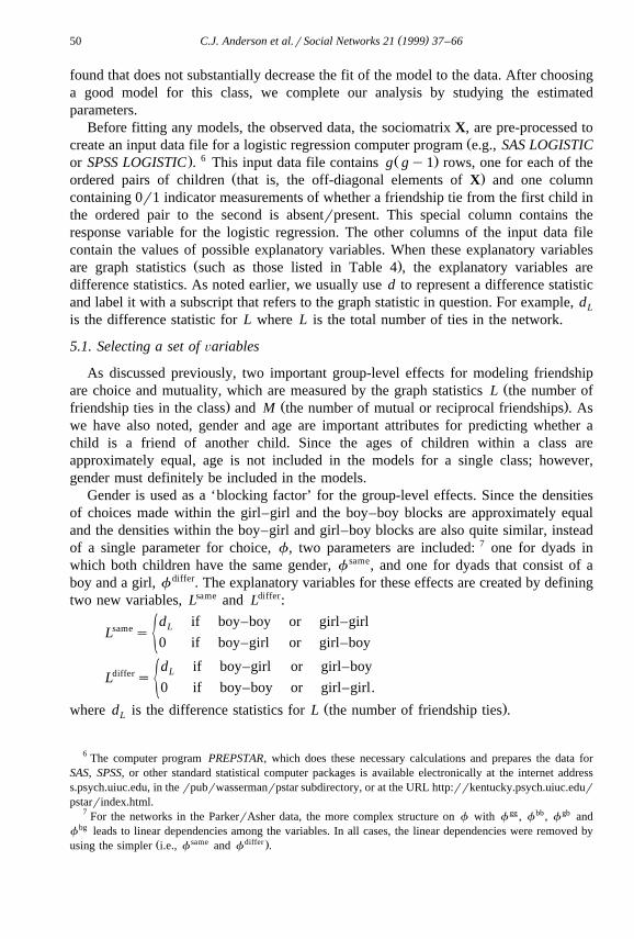
Gender is used as a ‘blocking factor’ for the group-level effects. Since the densitiesof choices made within the girl–girl and the boy–boy blocks are approximately equaland the densities within the boy–girl and girl–boy blocks are also quite similar, insteadof a single parameter for choice, f, two parameters are included: 7 one for dyads inwhich both children have the same gender, f same, and one for dyads that consist of aboy and a girl, f differ. The explanatory variables for these effects are created by definingtwo new variables, Lsame and Ldiffer:

d if boy–boy or girl–girlLsameL s ½0 if boy–girl or girl–boy

d if boy–girl or girl–boyLdifferL s ½0 if boy–boy or girl–girl.

Ž .where d is the difference statistics for L the number of friendship ties .L

6 The computer program PREPSTAR, which does these necessary calculations and prepares the data forSAS, SPSS, or other standard statistical computer packages is available electronically at the internet addresss.psych.uiuc.edu, in the rpubrwassermanrpstar subdirectory, or at the URL http:rrkentucky.psych.uiuc.edurpstarrindex.html.

7 For the networks in the ParkerrAsher data, the more complex structure on f with f gg , f bb, f gb andf bg leads to linear dependencies among the variables. In all cases, the linear dependencies were removed by

Ž same differ .using the simpler i.e., f and f .


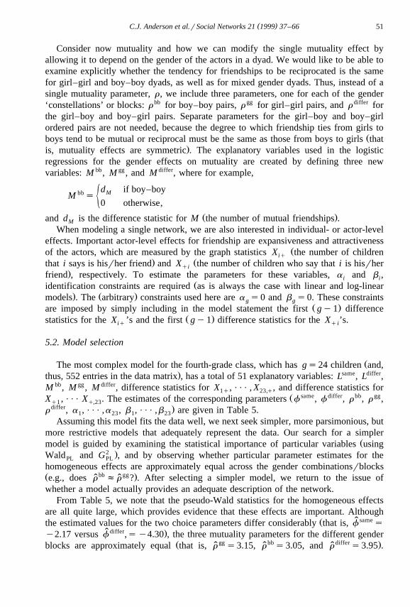
Consider now mutuality and how we can modify the single mutuality effect byallowing it to depend on the gender of the actors in a dyad. We would like to be able toexamine explicitly whether the tendency for friendships to be reciprocated is the samefor girl–girl and boy–boy dyads, as well as for mixed gender dyads. Thus, instead of asingle mutuality parameter, r, we include three parameters, one for each of the gender‘constellations’ or blocks: r bb for boy–boy pairs, r gg for girl–girl pairs, and r differ forthe girl–boy and boy–girl pairs. Separate parameters for the girl–boy and boy–girlordered pairs are not needed, because the degree to which friendship ties from girls to

Žboys tend to be mutual or reciprocal must be the same as those from boys to girls that.is, mutuality effects are symmetric . The explanatory variables used in the logistic

regressions for the gender effects on mutuality are created by defining three newvariables: M bb, M gg , and M differ, where for example,

d if boy–boyMbbM s ½0 otherwise,

Ž .and d is the difference statistic for M the number of mutual friendships .M

When modeling a single network, we are also interested in individual- or actor-leveleffects. Important actor-level effects for friendship are expansiveness and attractiveness

Žof the actors, which are measured by the graph statistics X the number of childreniq. Žthat i says is hisrher friend and X the number of children who say that i is hisrherqi

.friend , respectively. To estimate the parameters for these variables, a and b ,i iŽidentification constraints are required as is always the case with linear and log-linear

. Ž .models . The arbitrary constraints used here are a s0 and b s0. These constraintsg gŽ .are imposed by simply including in the model statement the first gy1 difference

Ž .statistics for the X ’s and the first gy1 difference statistics for the X ’s.iq qi

5.2. Model selection

ŽThe most complex model for the fourth-grade class, which has gs24 children and,. same differthus, 552 entries in the data matrix , has a total of 51 explanatory variables: L , L ,

M bb, M gg , M differ, difference statistics for X , PPP , X , and difference statistics for1q 23,qŽ same differ bb ggX , PPP X . The estimates of the corresponding parameters f , f , r , r ,q1 q,23

differ .r , a , PPP ,a , b , PPP ,b are given in Table 5.1 23 1 23

Assuming this model fits the data well, we next seek simpler, more parsimonious, butmore restrictive models that adequately represent the data. Our search for a simpler

Žmodel is guided by examining the statistical importance of particular variables using2 .Wald and G , and by observing whether particular parameter estimates for thePL PL

homogeneous effects are approximately equal across the gender combinationsrblocksŽ bb gg .e.g., does r fr ? . After selecting a simpler model, we return to the issue ofˆ ˆwhether a model actually provides an adequate description of the network.

From Table 5, we note that the pseudo-Wald statistics for the homogeneous effectsare all quite large, which provides evidence that these effects are important. Although

ˆ sameŽthe estimated values for the two choice parameters differ considerably that is, f sˆ differ .y2.17 versus f ,sy4.30 , the three mutuality parameters for the different gender

Ž gg bb differ .blocks are approximately equal that is, r s3.15, r s3.05, and r s3.95 .ˆ ˆ ˆ


Table 5Ž .Estimated parameters, approximate asymptotic standard errors, and pseudo-Wald statistics of the most

complex model fit to the 552 dyads from the friendship data for the fourth-grade class

Effect Explanatory Model Estimated Approximate WaldPL

variable parameter value standard errorsame sameChoice L f y2.17 1.15 3.53differ differL f y4.30 1.17 13.50

gg ggMutual M r 3.15 0.69 20.90bb bbM r 3.05 0.49 38.54differ differM r 3.95 0.72 30.43

Expansiveness X a 1.29 1.22 1.121q 1. . . . .. . . . .. . . . .X a 0.28 1.16 0.0623,q 23

X a 0.00 0.00 –24,q 24

Attractiveness X b y0.94 0.89 1.11q1 1. . . . .. . . . .. . . . .X b y0.35 0.92 0.15q,23 23

X b 0.00 0.00 –q,24 24

These observations suggest that restricting r gg sr bb sr differ will have a statisticallynegligible effect on the fit of the model, but that restricting f same sf differ will lead to alarge reduction in the goodness of fit. Confirmation of these conjectures is obtained fromthe pseudo-Wald statistics 8, Wald , and pseudo-likelihood ratio statistics 9, G2 , forPL PL

these restrictions on the parameters, which are reported in Table 6.Also reported in Table 6 are the pseudo-test statistics that assess the statistical

importance of expansiveness and attractiveness. Although each of the 23 parameters foreach effect could be examined, to assess whether the overall effect of expansiveness orattractiveness is important, the entire set of 23 parameters for either effect should beconsidered simultaneously. This goal is met by imposing the linear restriction a s PPP1

sa s0 for expansiveness and the linear restriction b s PPP sb s0 for popular-23 1 23

ity. In the absence of higher-order terms, the statistics in Table 6 provide evidence of thenecessity of both expansiveness and attractiveness.

The estimated parameters of the model with a single mutuality parameter are reportedin Table 7. While not reported here, we looked at even more restrictive models. TheWald and G2 statistics for these more restrictive models indicate that no furtherPL PL

simplifications should be made. At this point, another possibility is either to addŽ .higher-order terms e.g., transitivity or 2-stars or replace individual level terms with

higher-order ones. We fit such models later in Section 7. Before interpreting theestimated model, we need to assess how well this model actually represents thefriendship network of the fourth-graders.

8 Wald statistics for linear restrictions on parameters were obtained from the ‘TEST’ option available inSAS LOGISTIC.

9 2 Ž .The G statistics reported here equal the difference between y2 log likelihood for the restricted modelPL

and the more general model.


Table 6Pseudo-Wald and pseudo-likelihood ratio test statistics for various linear restrictions on the parameters of themost complex model

2Effect Test df Wald Prob G ProbPL PL

same differChoicerdensity f sf 1 30.04 -0.001 35.25 -0.001gg bbMutuality r s r 1 0.01 0.92 0.01 0.92gg bb differr s r s r 2 1.26 0.53 1.26 0.53

Expansiveness a s PPP s a s0 23 52.90 -0.001 67.90 -0.0011 23

Attractiveness b s PPP s b s0 23 43.75 -0.001 57.32 -0.0011 23

ˆIf the model fits the data well, then the predicted or estimated sociomatrix X based onthe modeled probabilities of ties should be similar to the observed sociomatrix X. A tie

ˆŽ .is predicted from child i to child j that is, X s1 when the predicted probability of ai j

tie from child i to j is greater than or equal to 0.5; specifically, we require

1cˆ <P X s1 X s G0.5.Ž .i j i j Xˆ1qexp yu d zŽ .i j

ˆ ˆ cŽ . Ž .No tie is predicted that is, X s0 when P X s1 X -0.5. Comparisons of thei j i j i j

observed and predicted ties are used here to assess both the global fit of the model andthe fit of the model to each child’s data.

Ž .Globally, the final model correctly predicts 85.7% 473 of the 552 elements of theŽ .sociomatrix. Equivalently, the overall error rate is only 14.3%. The presence absence

Ž .of a tie is incorrectly predicted 5.6% 8.7% of the time. To assess how well thefriendship nominations made and received by individual children are fit by the model,the row and column sums of the absolute value of the difference between the observed

ˆŽ < <.and predicted sociomatrices i.e., XyX , were computed. The row sums equal thenumber of errors made in reproducing the friendship nominations made by individual

Table 7Estimated parameters, approximate standard errors, and pseudo-Wald statistics for parameters of the simplestmodel

Effect Explanatory Parameter Standard Wald OddsPL

variable estimate error ratiosameChoice L y2.26 1.08 4.38 0.10differL y4.17 1.11 14.17 0.02

Mutuality M 3.27 0.37 79.22 26.31Expansiveness X 1.27 1.15 1.22 3.561q. . . . .. . . . .. . . . .

X 0.28 1.16 0.06 1.3223,qX 0.00 0.00 – 1.0024,q

Attractiveness X y0.86 0.88 0.96 0.42q1. . . . .. . . . .. . . . .X y0.36 0.91 0.15 0.70q,23

X 0.00 0.00 – 1.00q,24


Table 8Ž .The number of errors made the ‘stem’ out of a possible 552 in reproducing the friendship nominations made

Ž . Ž . Ž .‘senders’ and received ‘receivers’ by individual children the ‘leaves’

Senders Receivers

0 00 01 1 0 0 002 2 0 0 0 0 00 0 0 03 3 0 0 0 0 00 0 0 0 0 04 4 0 0 0 0 00 0 0 0 0 05 5 0 0 0 0 00 06 6 00...

011

Ž .children ‘senders’ and the column sums equal the number of errors made in reproduc-Ž .ing the friendship nominations received by each child ‘receivers’ . Stem-and-leaf

displays of these summed prediction errors for the senders and receivers are given inTable 8.

Ž .The friendship nominations made by one child a21 are not well modeled. Out ofthe 23 possible nominations made by this child, 11 of the predictions are incorrect.Inspection of the sociomatrix shows that of her nine friendship nominations, she choseseven boys and two girls. This pattern stands in contrast to the largely same-genderfriendships of the other children and is a major source of the lack-of-fit. 10 However, ourfinal model reproduces the observed sociomatrix rather well overall.

5.3. Model interpretation

When an estimated choice parameter is positive, the probability that a tie is present islarger than the probability that it is absent, conditional on all other effects in the model.Conversely, when a choice parameter is negative, it is more likely that a tie is absent

ˆ same ˆ differthan it is present. Since the two estimated parameters for choice, f and f , areŽboth negative, it is more likely that a tie is globally absent than present given the other

.effects in the model . Suppose we examine the density of the ties, measured as thefraction of ties actually present in the sociomatrix, Table 2. We see that the density ofties within same gender pairs is much greater than between gender pairs, as evidenced

ˆ same ˆ differby f being larger than f . Specifically, the odds that a tie is present given thatŽ Ž .. Ž .two children are both girls or both boys is exp y2.26y y4.17 sexp 1.91 s6.75

times larger than the odds when one child is a boy and the other is a girl.Ž .With respect to mutuality, the odds that a tie is present versus absent is exp 3.27 s

26.3 times greater due to the tendency for friendships to be reciprocated. Furthermore,because the restriction that r bb sr gg sr differ did not affect the fit of the model, thistendency toward mutual friendships does not depend on the gender constellation of thedyads.

10 The models fit in Section 7 where the individual effects in the models are replaced by higher-order termshave comparable fits and do not have any outliers.


Two individual-level parameters are estimated for each child. The odds that a tie isŽ .Xpresent from child i to j because of the expansiveness of the ‘chooser’ is exp a yaˆ ˆi i

times the odds that a tie is present from child iX to j. Given the arbitrary identificationŽ . Ž .constraint for the expansiveness parameters i.e., a s0 , exp a indicates how manyˆ24 i

times larger the odds that a tie is present from child i to j is relative to the odds forchild 24. The larger the estimated value of a , the larger the odds that child i nominatesi

other children as friends. The expansiveness parameters are measures of the tendency ofchildren to nominate others, while holding all other effects in the model constant.

With respect to attractiveness, the odds that a tie is present from child i to j becauseˆ ˆŽ .Xthe attractiveness of the ‘chosen’ is exp b yb times the odds that a tie is presentj j

from child i to jX. The larger the estimated value of b , the greater the odds that a childj

chooses j as a friend. The attractiveness parameters are measures of ‘popularity’ anddepict essentially the same construct as the acceptance ratings that were also collectedfor the children in this class; however, the attractiveness parameters also take intoconsideration the tendencies toward expansiveness, mutuality, and density.

6. Extensions of logit pU to multiple networks

The Parker and Asher classrooms are an example of a multiple network data set. Wehave relations defined for several sets of actors, but no relational ties recorded across thesets. In other words, the friendship ties that the third-graders have with the fifth-graders,or more generally, friendship ties that span classrooms, are not recorded. Nonetheless, itis of interest to analyze these multiple networks simultaneously to study differencesamong the grades.

Given the single-classroom analysis just presented, we might wonder whether thetendencies toward mutuality are the same across networksrclasses or whether otherhomogeneous effects have a similar strength across classes. Fitting separate models tothe classes does not allow us to address this question; we need to fit all the classes in asingle analysis so that we can place equality restrictions on parameters across models.

Ž .We can use the acceptance ratings acceptance =d in lieu of attractiveness parame-j L

ters and use the loneliness scores of senders and receivers, which are the closest weŽ .come to individual-level effects in these models for reasons described below .

It is straightforward to extend pU to this multiple network situation. We first create anew multiple network relation, XX Žm., which is the aggregation of the relations definedon each of the individual networks. Suppose there are N networks, with actor sets NN ,1

NN , PPP , NN , of sizes g , g , PPP , g , respectively. We assume the same relation is2 N 1 2 N

measured on each network—otherwise, it makes little sense to analyze the networkssimultaneously. Further, relational ties are only allowed within sets—children only haveties to other children within the same classroom. 11

11 We note however, that techniques for modeling multiple networks in which actors are allowed to haveŽ .relational ties to actors in other actor sets have been described by Iacobucci and Wasserman 1990 and

Ž .Wasserman and Iacobucci 1991 .


We create a multiple network, with actor set NN Žm.sNN jNN j PPP jNN , and1 2 N

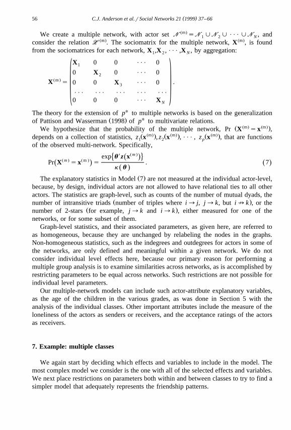
consider the relation XX Žm.. The sociomatrix for the multiple network, X Žm., is foundfrom the sociomatrices for each network, X ,X , PPP ,X , by aggregation:1 2 N

X 0 0 PPP 01

0 X 0 PPP 02Žm .X s .0 0 X PPP 03

PPP PPP PPP PPP PPP� 00 0 0 PPP X N

The theory for the extension of pU to multiple networks is based on the generalizationŽ . Uof Pattison and Wasserman 1998 of p to multivariate relations.

Ž Žm. Žm..We hypothesize that the probability of the multiple network, Pr X sx ,Ž Žm.. Ž Žm.. Ž Žm..depends on a collection of statistics, z x , z x , PPP , z x , that are functions1 2 p

of the observed multi-network. Specifically,X Ž .mexp u z x� 4Ž .Ž . Ž .m mPr X sx s . 7Ž .Ž .

k uŽ .Ž .The explanatory statistics in Model 7 are not measured at the individual actor-level,

because, by design, individual actors are not allowed to have relational ties to all otheractors. The statistics are graph-level, such as counts of the number of mutual dyads, the

Ž .number of intransitive triads number of triples where i™ j, j™k, but i¢k , or theŽ .number of 2-stars for example, j™k and i™k , either measured for one of the

networks, or for some subset of them.Graph-level statistics, and their associated parameters, as given here, are referred to

as homogeneous, because they are unchanged by relabeling the nodes in the graphs.Non-homogeneous statistics, such as the indegrees and outdegrees for actors in some ofthe networks, are only defined and meaningful within a given network. We do notconsider individual level effects here, because our primary reason for performing amultiple group analysis is to examine similarities across networks, as is accomplished byrestricting parameters to be equal across networks. Such restrictions are not possible forindividual level parameters.

Our multiple-network models can include such actor-attribute explanatory variables,as the age of the children in the various grades, as was done in Section 5 with theanalysis of the individual classes. Other important attributes include the measure of theloneliness of the actors as senders or receivers, and the acceptance ratings of the actorsas receivers.

7. Example: multiple classes

We again start by deciding which effects and variables to include in the model. Themost complex model we consider is the one with all of the selected effects and variables.We next place restrictions on parameters both within and between classes to try to find asimpler model that adequately represents the friendship patterns.


The homogeneous effects listed in Table 4 that are likely to be important andinteresting for modeling friendship relations are choice, mutuality, degree centralization,degree group prestige, transitivity, cyclicity, 2-in-stars, 2-out-stars, and 2-mixed-stars.Degree centralization and prestige are quantified here as the variance of the number of

Ž . Ž .choices made X and the variance of the number of choices received X ,iq qi

respectively. Transitivity, cyclicity, and 2-stars are graph statistics measured on tripletsof actors. Transitivity and cyclicity are two specific patterns of ties in which 3 ties arepresent, while the various 2-stars are different patterns involving 2 ties. A triplet ofactors may exhibit either one, none, or all these effects. For example, the transitivitystatistic, which equals the number of triples where child i™ j, j™k and i™k, is

Ž . Ž .composed of a 2-in-star j™k and i™k , a 2-out-star i™ j and i™k , and aŽ .2-mixed-star i™ j and j™k .

Previous research has indicated that age is an important factor in accounting forŽ .friendships Parker and Asher, 1993 ; however, we do not explicitly include age in our

analyses here. Since ages of children within the same grade level are approximatelyequal and we are only analyzing one classroom from each of the three grade levels, ageis confounded with classroom. Our goal here is to demonstrate how pU can be used to

Ž .analyze multiple networks. To tease apart effects resulting from age or grade level andŽclasses requires the use of multiple classes from each grade level i.e., use of all 36

.networks from the Parker and Asher data .Gender is once again used as a blocking factor for the homogeneous effects. Gender

effects on choice and mutuality are handled as they were in the analysis of the singleclass. For the remaining homogeneous effects, four possible parameters are included in

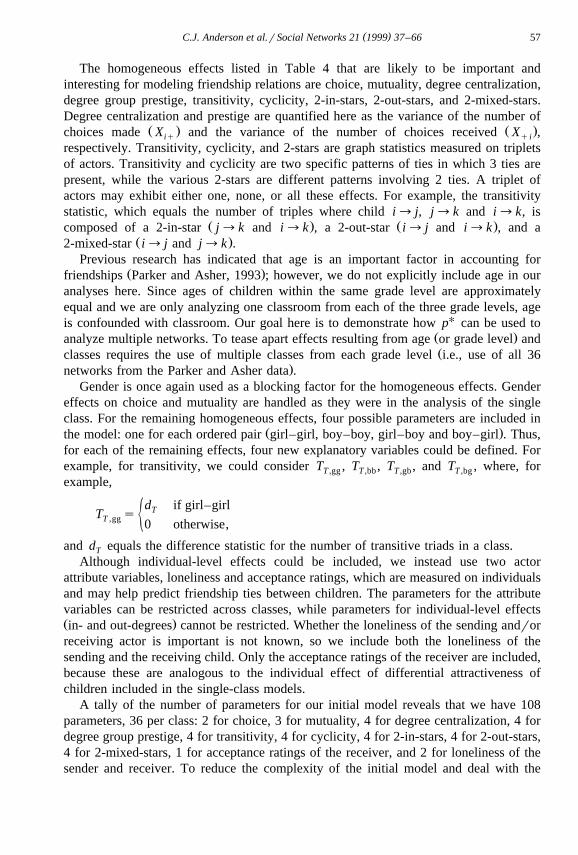
Ž .the model: one for each ordered pair girl–girl, boy–boy, girl–boy and boy–girl . Thus,for each of the remaining effects, four new explanatory variables could be defined. Forexample, for transitivity, we could consider T , T , T , and T , where, forT ,gg T ,bb T ,gb T ,bg

example,

d if girl–girlTT sT ,gg ½0 otherwise,

and d equals the difference statistic for the number of transitive triads in a class.T

Although individual-level effects could be included, we instead use two actorattribute variables, loneliness and acceptance ratings, which are measured on individualsand may help predict friendship ties between children. The parameters for the attributevariables can be restricted across classes, while parameters for individual-level effectsŽ .in- and out-degrees cannot be restricted. Whether the loneliness of the sending androrreceiving actor is important is not known, so we include both the loneliness of thesending and the receiving child. Only the acceptance ratings of the receiver are included,because these are analogous to the individual effect of differential attractiveness ofchildren included in the single-class models.

A tally of the number of parameters for our initial model reveals that we have 108parameters, 36 per class: 2 for choice, 3 for mutuality, 4 for degree centralization, 4 fordegree group prestige, 4 for transitivity, 4 for cyclicity, 4 for 2-in-stars, 4 for 2-out-stars,4 for 2-mixed-stars, 1 for acceptance ratings of the receiver, and 2 for loneliness of thesender and receiver. To reduce the complexity of the initial model and deal with the


Žpractical difficulties that arise when working with a model with 108 parameters i.e.,.defining all of the variables and keeping track of them , we use the fact that when no

restrictions are placed on parameters across classes, the distributions for the individualclassrooms are statistically independent. Thus, the model with 108 parameters fitsimultaneously to all classes is equivalent to fitting the 36-parameter model to each classseparately. The three models, one fitted to each class separately, yield the sameestimated parameters and fit statistics of the overall model. The overall fit statistic is thesum of the three statistics from each class.

Thus, in the first round of simplifications, we start with the same model for each classand place restrictions on parameters within classes. In the next round, restrictionsbetween classes are imposed. In this second round, the restrictions test whether separateparameters are needed for the different classes, as well as whether further restrictionswithin classes are possible.

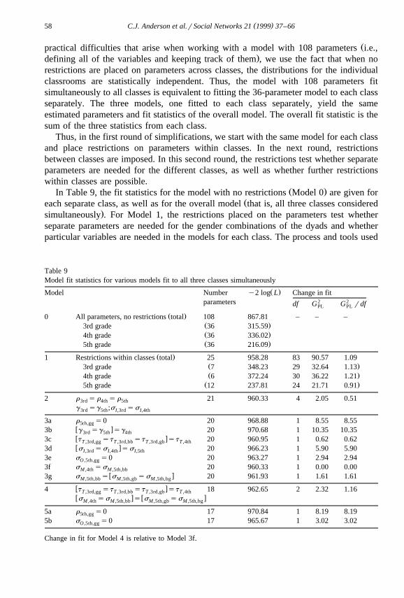
Ž .In Table 9, the fit statistics for the model with no restrictions Model 0 are given forŽeach separate class, as well as for the overall model that is, all three classes considered

.simultaneously . For Model 1, the restrictions placed on the parameters test whetherseparate parameters are needed for the gender combinations of the dyads and whetherparticular variables are needed in the models for each class. The process and tools used

Table 9Model fit statistics for various models fit to all three classes simultaneously

Ž .Model Number y2 log L Change in fit2 2parameters df G G rdfPL PL

Ž .0 All parameters, no restrictions total 108 867.81 – – –Ž .3rd grade 36 315.59Ž .4th grade 36 336.02Ž .5th grade 36 216.09

Ž .1 Restrictions within classes total 25 958.28 83 90.57 1.09Ž .3rd grade 7 348.23 29 32.64 1.13Ž .4th grade 6 372.24 30 36.22 1.21Ž .5th grade 12 237.81 24 21.71 0.91

2 r s r s r 21 960.33 4 2.05 0.513rd 4th 5th

g sg ;s ss3rd 5th I,3rd I,4th

3a r s0 20 968.88 1 8.55 8.555th,ggw x3b g sg sg 20 970.68 1 10.35 10.353rd 5th 4thw x3c t st st st 20 960.95 1 0.62 0.62T ,3rd,gg T ,3rd,bb T ,3rd,gb T ,4thw x3d s ss ss 20 966.23 1 5.90 5.90I,3rd I,4th I,5th

3e s s0 20 963.27 1 2.94 2.94O ,5th,gg

3f s ss 20 960.33 1 0.00 0.00M ,4th M ,5th,bbw x3g s s s ss 20 961.93 1 1.61 1.61M ,5th,bb M ,5th,gb M ,5th,bg

w x4 t st st st 18 962.65 2 2.32 1.16T ,3rd,gg T ,3rd,bb T ,3rd,gb T ,4thw x w xs ss s s ssM ,4th M ,5th,bb M ,5th,gb M ,5th,bg

5a r s0 17 970.84 1 8.19 8.195th,gg

5b s s0 17 965.67 1 3.02 3.02O ,5th,gg

Change in fit for Model 4 is relative to Model 3f.


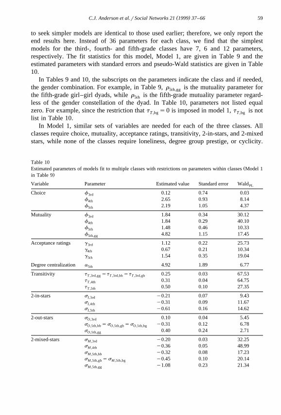
to seek simpler models are identical to those used earlier; therefore, we only report theend results here. Instead of 36 parameters for each class, we find that the simplestmodels for the third-, fourth- and fifth-grade classes have 7, 6 and 12 parameters,respectively. The fit statistics for this model, Model 1, are given in Table 9 and theestimated parameters with standard errors and pseudo-Wald statistics are given in Table10.

In Tables 9 and 10, the subscripts on the parameters indicate the class and if needed,the gender combination. For example, in Table 9, r is the mutuality parameter for5th,gg

the fifth-grade girl–girl dyads, while r is the fifth-grade mutuality parameter regard-5th

less of the gender constellation of the dyad. In Table 10, parameters not listed equalzero. For example, since the restriction that t s0 is imposed in model 1, t is notT ,bg T ,bg

list in Table 10.In Model 1, similar sets of variables are needed for each of the three classes. All

classes require choice, mutuality, acceptance ratings, transitivity, 2-in-stars, and 2-mixedstars, while none of the classes require loneliness, degree group prestige, or cyclicity.

Table 10ŽEstimated parameters of models fit to multiple classes with restrictions on parameters within classes Model 1

.in Table 9

Variable Parameter Estimated value Standard error WaldPL

Choice f 0.12 0.74 0.033rd

f 2.65 0.93 8.144th

f 2.19 1.05 4.375th

Mutuality f 1.84 0.34 30.123rd

f 1.84 0.29 40.104th

f 1.48 0.46 10.335th

f 4.82 1.15 17.455th,gg

Acceptance ratings g 1.12 0.22 25.733rd

g 0.67 0.21 10.344th

g 1.54 0.35 19.045th

Degree centralization a 4.92 1.89 6.775th

Transitivity t st st 0.25 0.03 67.53T ,3rd,gg T ,3rd,bb T ,3rd,gb

t 0.31 0.04 64.75T ,4th

t 0.50 0.10 27.35T ,5th

2-in-stars s y0.21 0.07 9.43I,3rd

s y0.31 0.09 11.67I,4th

s y0.61 0.16 14.62I,5th

2-out-stars s 0.10 0.04 5.45O ,3rd

s ss ss y0.31 0.12 6.78O ,5th,bb O ,5th,gb O ,5th,bg

s 0.40 0.24 2.71O ,5th,gg

2-mixed-stars s y0.20 0.03 32.25M ,3rd

s y0.36 0.05 48.99M ,4th

s y0.32 0.08 17.23M ,5th,bb

s ss y0.45 0.10 20.14M ,5th,gb M ,5th,bg

s y1.08 0.23 21.34M ,5th,gg


Degree centralization is important only for the fifth-grade class, and 2-out-stars isimportant for the third- and fifth-grade classes. Gender is required primarily for thefifth-grade friendships, especially for girl–girl dyads but is also needed for transitivity inthe third grade.

Ž .Fitting a single model to all three classes simultaneously with or without restrictionson parameters across classes requires that the data for each of the three classes be

Žcombined into a single file. For our example, the combined data file contains g g3rd 3rd. Ž . Ž .y1 qg g y1 qg g y1 rows, one line of data for each of the ordered4th 4th 5th 5th

pairs. This combined file also has a single indicator variable indicating whether a tieexists between pairs of children which is our response variable in the logistic regression.

To allow parameters to differ across classes, a separate variable for a particular effectfor each class is needed. For example, to allow the parameter for mutuality to differacross the classes requires three variables: d , d , and d , that are defined, forM ,3rd M ,4th M ,5th

example, as

d for third-grade classMd sM ,3rd ½0 otherwise,

Ž . 12where d is the difference statistic for mutuality, regardless of class or gender . ToM

restrict parameters to be equal over classes, a single variable is used. For example, oneof the restrictions imposed here is that the parameters for 2-in-stars for the third- andfourth-grades are equal, but not necessarily equal to that for the fifth-grade. Thevariables needed for this are

d if third- or fourth-gradeSId sS ,3&4I ½0 otherwise

d if fifth-gradeSId sS ,5thI ½0 otherwise,

where d is the difference statistics for 2-in-stars.SI

Possible restrictions across classes are suggested by the values of some of theestimated parameters in Table 10. We look for equalities within the parameter types. Forexample, the estimated values for mutuality for the three grades are r s1.84,r sˆ ˆ3rd 4th

1.84 and r s1.48. As was done with the models for the single class, possible linearˆ5th

restrictions were first examined using the pseudo-Wald statistics. The restrictions,r sr sr , g sg , and s ss , yield Wald statistics that are clearly3rd 4th 5th 3rd 5th I,3rd I,4th PL

‘small’ and are the smallest among the various restrictions tried. Imposing these threeŽrestrictions leads to a small decrease in the overall fit of the model that is, for Model 2,

2 Ž . Ž . .using statistics given in Table 9, G rdfs 960.33y958.28 r 25y1 s2.05r4s0.5 ;pl

therefore, these restrictions are adopted.Based on the estimated parameters of Model 2, additional restrictions appear to be

possible. Various models with one additional restriction, Models 3a–3g in Table 9, were

12 As a check of whether the data file and variables are correctly defined, we recommend that the simplestmodel found when fitting models to each class separately be fit using the combined data file. In our example,this is Model 1.


fit. Restrictions already in effect for each of these models are those given withinw xbrackets . For example, the restriction s ss was adopted in Model 2, and theI,3rd I,4th

additional restriction imposed by Model 3d is that the common value for the third andw xfourth grades equals that value for the fifth grade class, s ss ss .I,3rd I,4th I,5th

Because the restriction in Model 3f, s ss , has nearly no effect on the fitM ,3rd M ,5th,bb

of the model, it is included in all further models. Additional restrictions that have only aŽ .small effect are imposed in Models 3c transitivity for third- and fourth-grades and 3g

Žin the fifth-grade, the parameter for 2-mixed-stars for the boy–boy dyads is equal to.that for boy–girl and girl–boy dyads . Note that this restriction for Model 3g is a

within-class restriction that was previously tested when classes were analyzed sepa-rately; however, given the restrictions over classes adopted in Model 2, this within-class

Ž .restriction is no longer statistically important.Model 4 is the same as Model 3f with the additional restrictions imposed by both

Ž 2Models 3c and 3g. Because the change in fit is relatively small that is, G rdfsPL.2.32r2s1.1 , all these restrictions are adopted. For our last attempt to simplify the

model, two additional restrictions are imposed; however, each of these yields a relativelylarge G2 rdf , indicating that the restrictions substantially decrease the fit of the model.PL

As a final step, the same error analysis performed earlier is performed here on Model 4.Ž .Overall, Model 4 correctly reproduces 86.7% 1280 of the possible 1476 ties and

correctly reproduces 83.1%, 86.6% and 90.0% of the ties in the third-, fourth- andfifth-grade classes, respectively. Furthermore, no outliers or patterns in the residualswere detected.

The estimated parameters and their standard errors for Model 4, our final model, arereported in Table 11. The numbers in the last column of this table, labeled ‘Odds ratio’,are the exponential of the estimated parameters. These quantities provide an indicationof the impact of the variable associated with a particular row on the modeled odds that atie is present. We do not interpret the choice parameters here, because they areanalogous to means within classes and because we think that the estimated odds ratiosare easier to understand.

Regardless of gender and grade, the tendency toward mutuality is important. TheŽ .odds of a tie being present are exp 1.81 s6.12 times larger than when the tie is absent

because of the tendency toward reciprocal friendships. In the fifth-grade, the odds that atie is present for girl–girl dyads resulting from mutuality is an additional 15.55 timeslarger than the odds in the other two classes or the odds for other gender constellationsin the fifth grade. Centralization is also important in the fifth-grade. The odds that a tie

Ž .is present because of centralization is a very large 79.39 times larger in the fifth-gradethan the odds in the other grades. Acceptance ratings are an important factor in allclasses. In the third- and fifth-grades, the predicted odds of a tie is 3.73 times largergiven a 1 unit increase in a child’s acceptance rating. In the fourth-grade, the fitted oddsratio for a 1 unit increase is 1.87.

The effects defined on triplets of actors, transitivity and the ‘2-star’ effects, bothincrease and decrease the odds that a tie is present. For all classes, transitivity leads toan increase in the predicted odds of a tie; specifically, the odds ratio for the third-gradeboy–boy, girl–girl and girl–boy dyads and for all gender combinations in the fourth-grade equals 1.33, and in the fifth-grade, the odds ratio equals 1.73. Thus, transitive


Table 11Ž .Estimated parameters of multiple class model Model 4 in Table 9

Variable Parameter Estimated Standard Oddsvalue error ratio

Choice f 0.54 0.68 1.713rd

f 2.56 0.58 12.964th

f 1.44 0.74 4.225th

Mutuality r s r s r 1.81 0.20 6.123rd 4th 5th

r 2.74 1.10 15.555th,gg

Degree Centralization a 4.37 1.78 79.395th

Acceptance g sg 1.32 0.17 3.733rd 5th

Ratings g 0.62 0.17 1.874th

Transitivity t st st st 0.28 0.02 1.33T ,3rd,gg T ,3rd,bb T ,3rd,gb T ,4th

t 0.55 0.06 1.73T ,5th

In-2-Stars s ss y0.27 0.05 0.76I,3rd I,4th

s y0.53 0.11 0.59I,5th

Out-2-Stars s 0.09 0.04 1.10O ,3rd

s ss ss y0.27 0.10 0.76O ,5th,bb O ,5th,gb O ,5th,bg

s 0.38 0.24 1.47O ,5th,gg

Mixed-2-Stars s y0.20 0.03 0.82M ,3rd

s ss ss ss y0.35 0.04 0.70M ,4th M ,5th,bb M ,5th,gb M ,5th,bg

s y0.99 0.21 0.37M ,5th,gg

friendships increase the odds of friendship ties. For the most part, the increases in2-in-stars, 2-out-stars, and 2-mixed-stars tend to increase the probabilities that friendshipties are absent, except for girl–girl friendships in the fifth-grade.

8. Conclusions and extensions

The pU model for a single social network and the multiple network extensionintroduced here overcome the severely limiting assumption of independence on dyadsmade by earlier statistical models for such data. Since pU and the multi-networkgeneralization are simply logistic regressions, they are easily fit to data using standardstatistical computing packages.

The novel feature of the multiple network pU model is that it allows researchers tofind communalities and similarities among networks under study, while also allowing

Žfor uniquenesses and idiosyncrasies within networks borrowing from the language of.factor analysis . Individual networks have their own ‘personalities’, which can easily be

.found by studying the differences among the networks , but they also share commonŽ .structural aspects. Communalities between networks suggest imply that underlying

processes generating relational ties are similar. Thus, multi-network pU provides astatistical tool to study these possible underlying processes.

The flexibility of the pU modeling approach was demonstrated by its extensions toŽmultiple relations and valued relations Pattison and Wasserman, 1998; Robins et al.,


. U1998 , and the multi-network p introduced here, which also incorporated actorattributes. New model developments permit the prediction and modeling of actor

Ž . Ž .attributes such as loneliness from relational variables such as friendship . A first stepŽ .toward such models is given by Robins 1997 .

Acknowledgements

This research was supported by grants from the National Science FoundationŽ .aSBR96-17510 and aSBR96-30754 , from the National Institutes of Health, and theBureau of Educational Research at the University of Illinois. We thank Jeff Parker andSteve Asher for providing us with the data described and used here, Phipps Arabie, PipPattison, Michelle Perry and Razia Azen for comments on this research, and FeliciaTrachtenberg for comments and research assistance.

References

Agresti, 1990. Categorical Data Analysis. Wiley, New York.Agresti, A., 1996. An Introduction to Categorical Data Analysis. Wiley, New York.

Ž .Arabie, P., Boorman, S.A., 1982. Blockmodels: developments and prospects. In: Hudson, H.C. Ed. ,Classifying Social Data. Jossey-Bass, San Francisco.

Arabie, P., Boorman, S.A., Levitt, P.R., 1978. Constructing blockmodels: how and why. Journal of Mathemat-ical Psychology 17, 21–63.

Arabie, P., Hubert, L.J., 1992. Combinatorial data analysis. Annual Review of Psychology 43, 169–203.Arrow, H., 1994. Mapping the Structural Dynamics of Groups: Patterns of Leadership and Influence in Times

of Stability and Change. Department of Psychology, University of Illinois. Unpublished masters disserta-tion.

Arrow, H., 1997. Stability, bistability, and instability in small group influence patterns. Journal of Personalityand Social Psychology 72, 75–85.

Asher, S.R., Hymel, S., Renshaw, P.D., 1984. Loneliness in children. Child Development 55, 1456–1464.Asher, S.R., Wheeler, V.A., 1985. Children’s loneliness: a comparison of rejected and neglected peer status.

Journal of Counseling and Clinical Psychology 53, 500–505.Besag, J.E., 1972. Nearest-neighbour systems and the auto-logistic model for binary data. Journal of the Royal

Statistical Society, Series B 34, 75–83.Ž .Besag, J.E., 1974. Spatial interaction and the statistical analysis of lattice systems with discussion . Journal of

the Royal Statistical Society, Series B 36, 192–236.Besag, J.E., 1977. Some methods of statistical analysis for spatial data. Bulletin of the International Statistical

Association 47, 77–92.Boorman, S.A., White, H.C., 1976. Social structure from multiple networks: II. Role structures. American

Journal of Sociology 81, 1384–1446.Breiger, R.L., Boorman, S.A., Arabie, P., 1975. An algorithm for clustering relational data with applications to

social network analysis and comparison with multidimensional scaling. Journal of Mathematical Psychol-ogy 12, 328–383.

Cressie, N., 1991. Statistics for Spatial Data. Wiley, New York.Davis, J.A., 1967. Clustering and structural balance in graphs. Human Relations 20, 181–187.Davis, J.A., 1970. Clustering and hierarchy in interpersonal relations: testing two theoretical models on 742

sociograms. American Sociological Review 35, 843–852.Davis, J.A., 1979. The DavisrHollandrLeinhardt studies: An overview. In: Holland, P.W., Leinhardt, S.

Ž .Eds. , Perspectives on Social Network Research. Academic Press, New York, pp. 51–62.


Davis, J.A., Leinhardt, S., 1972. The structure of positive interpersonal relations in small groups. In: Berger, J.Ž .Ed. , Sociological Theories in Progress, Vol. 2. Houghton-Mifflin, Boston, pp. 218–251.

Ž .Diggle, P.J., 1996. Spatial analysis in biometry. In: Armitage, P., David, H.A. Eds. , Advances in Biometry.Wiley, New York, pp. 363–393.

Fienberg, S.E., Wasserman, S., 1981. Categorical data analysis of single sociometric relations. In: Leinhardt,Ž .S. Ed. , Sociological Methodology. Jossey-Bass, San Francisco, pp. 156–192.

Fienberg, S.E., Meyer, M.M., Wasserman, S., 1985. Statistical analysis of multiple sociometric relations.Journal of the American Statistical Association 80, 51–67.

Frank, O., 1991. Statistical analysis of change in networks. Statistica Neerlandica 45, 283–293.Frank, O., Nowicki, K., 1993. Exploratory statistical analysis of networks. Annals of Discrete Mathematics 55,

349–366.Frank, O., Strauss, D., 1986. Markov graphs. Journal of the American Statistical Association 81, 832–842.Galaskiewicz, Wasserman, S., 1989. Mimetic and normative processes within an interorganizational field: an

empirical test. Administrative Science Quarterly 34, 454–480.Galaskiewicz, J., Wasserman, S., 1990. Social action models for the study of change in organizational fields.

Ž .In: Weesie, J., Flap, H. Eds. , Social Networks Through Time. ISORrUniversity of Utrecht Press,Utrecht, The Netherlands, pp. 1–30.

Geyer, C.J., Thompson, E.A., 1992. Constrained Monte Carlo maximum likelihood for dependent data. Journalof the Royal Statistical Society. Series B 54, 657–699, with discussion.

Griffeath, D., 1979. Additive and Cancellative Interacting Particle Systems. Lecture Notes in Mathematics724. Springer, New York.

Holland, P.W., Leinhardt, S., 1970. A method for detecting structure in sociometric data. American Journal ofSociology 70, 492–513.

Holland, P.W., Leinhardt, S., 1971. Transitivity in structural models of small groups. Comparative GroupStudies 2, 107–124.

Holland, P.W., Leinhardt, S., 1972. Some evidence on the transitivity of positive interpersonal sentiment.American Journal of Sociology 72, 1205–1209.

Holland, P.W., Leinhardt, S., 1975. The statistical analysis of local structure in social networks. In: Heise,Ž .D.R. Ed. , Sociological Methodology 1976. Jossey-Bass, San Francisco, pp. 1–45.

Holland, P.W., Leinhardt, S., 1977. Notes on the statistical analysis of social network data.Holland, P.W., Leinhardt, S., 1978. An omnibus test for social structure using triads. Sociological Methods

and Research 7, 227–256.Ž .Holland, P.W., Leinhardt, S., 1979. Structural sociometry. In: Holland, P.W., Leinhardt, S. Eds. , Perspec-

tives on Social Network Research. Academic Press, New York, pp. 63–83.Holland, P.W., Leinhardt, S., 1981. An exponential family of probability distributions for directed graphs.

Journal of the American Statistical Association 76, 33–65, with discussion.Iacobucci, D., Wasserman, S., 1990. Social networks with two sets of actors. Psychometrika 55, 707–720.Ising, E., 1925. Beitrag zur theorie des ferromagnetismus. Zeitschrift fur Physik 31, 253–258.Kindermann, R.P., Snell, J.L., 1980. On the relation between Markov random fields and social networks.

Journal of Mathematical Sociology 8, 1–13.Koehly, L., 1996. Statistical Modeling of Congruence between Perceptual and Complete Networks. Unpub-

lished doctoral dissertation, Department of Psychology, University of Illinois.Krackhardt, D., 1987. Cognitive social structures. Social Networks 9, 109–134.Kumbasar, E., Romney, A.K., Batchelder, W.H., 1994. Systematic biases in social perception. American

Journal of Sociology 100, 477–505.Leinhardt, S., 1972. Developmental change in the sentiment structure of children’s groups. American

Sociological Review 37, 202–212.Leinhardt, S., 1973. The development of transitive structure in children’s interpersonal relations. Behavioral

Science 12, 260–271.Lorrain, F., White, H.C., 1971. Structural equivalence of individuals in social networks. Journal of Mathemati-

cal Sociology 1, 49–80.Parker, J.G., Asher, S.R., 1993. Friendship and friendship quality in middle childhood: Links with peer group

acceptance and feelings of loneliness and social dissatisfaction. Developmental Psychology 29, 611–621.Pattison, P.E., 1993. Algebraic Models for Social Networks. Cambridge University Press, Cambridge, UK.


Pattison, P.E., 1994. Social cognition in context: some applications of social network analysis. In: Wasserman,Ž .S., Galaskiewicz, J. Eds. , Advances in Social Network Analysis: Research from the Social and

Behavioral Sciences. Sage, Newbury Park, CA, pp. 79–109.Pattison, P., Wasserman, S., 1998. Logit models and logistic regressions for social networks: II. Multivariate

relations. To appear in British Journal of Mathematical and Statistical Psychology.Preston, C.J., 1974. Gibbs States on Countable Sets. Cambridge University Press, Cambridge, UK.

Ž .Rennolls, K., 1995. p . In: Everett, M.G., Rennolls, K. Eds. , Proceedings of the 1995 International1r2

Conference on Social Networks. Greenwich University Press, London, 1, pp. 151–160.Ripley, B.D., 1981. Spatial Statistics. Wiley, New York.Robins, G., 1997. pU models of social influence. Unpublished manuscript.Robins, G., Pattison, P., Langan-Fox, J., 1995. Group effectiveness: a comparative analysis of interactional

structure and performance in organizational workgroups. Paper presented at the International Network forSocial Network Analysis Annual Meeting. London, UK, July 1995.

Robins, G., Pattison, P.E., Wasserman, S., 1998. Logit models and logistic regressions for social networks: III.Valued relations. To appear in Psychometrika.

Speed, T.P., 1978. Relations between models for spatial data, contingency tables, and Markov fields ongraphs. Supplement Advances in Applied Probability 10, 11–122.

Strauss, D., 1977. Clustering on colored lattices. Journal of Applied Probability 14, 135–143.Strauss, D., 1986. On a general class of models for interaction. SIAM Review 28, 513–527.Strauss, D., 1992. The many faces of logistic regression. American Statistician 46, 321–327.Strauss, D., Ikeda, M., 1990. Pseudolikelihood estimation for social networks. Journal of the American

Statistical Association 85, 204–212.Walker, M.E., 1995. Statistical Models for Social Support Networks: Application of Exponential Models to

Undirected Graphs with Dyadic Dependencies. Unpublished doctoral dissertation, Department of Psychol-ogy, University of Illinois.

Walker, M., Wasserman, S., Wellman, B., 1993. Statistical models for social support networks. SociologicalMethods and Research 22, 71–98.

Wang, Y.J., Wong, G.Y., 1987. Stochastic blockmodels for directed graphs. Journal of the AmericanStatistical Association 83, 8–19.

Wasserman, S., 1978. Models for binary directed graphs and their applications. Advances in AppliedProbability 10, 803–818.

Wasserman, S., 1987. Conformity of two sociometric relations. Psychometrika 52, 3–18.Wasserman, S., Faust, K., 1994. Social Network Analysis: Methods and Applications. Cambridge University

Press, New York.Ž .Wasserman, S., Galaskiewicz, J. Eds. , 1994. Advances in Social Network Analysis, Research from the Social

and Behavioral Sciences. Sage, Newbury Park, CA.Wasserman, S., Iacobucci, D., 1988. Sequential social network data. Psychometrika 53, 261–282.Wasserman, S., Iacobucci, D., 1991. Statistical modeling of one-mode and two-mode networks: Simultaneous

analysis of graphs and bipartite graphs. British Journal of Mathematical and Statistical Psychology 44,13–44.

Wasserman, S., Pattison, P., 1996. Logit models and logistic regressions for social networks: I. Anintroduction to Markov random graphs and pU. Psychometrika 60, 401–426.

Wasserman and Pattison, 1997.Wasserman, S., Weaver, S., 1985. Statistical analysis of binary relational data: parameter estimation. Journal

of Mathematical Psychology 29, 406–427.Ž .Wellman, B., 1983. Network analysis: Some basic principles. In: Collins, R. Ed. , Sociological Theory, 1983.

Jossey-Bass, San Francisco, pp. 155–199.Ž .Wellman, B., Berkowitz, S.D. Eds. , 1997a. Social Structures: A Network Approach, Second Edition. JAI

Press, Greenwich, CT.Wellman, B., Berkowitz, S.D., 1997b. Introduction: Studying social structures. In: Wellman, B., Berkowitz,

Ž .S.D. Eds. , Social Structures: A Network Approach, Second Edition. JAI Press, Greenwich, CT, pp. 1–14.Wellman, B., Carrington, P.J., Hall, A., 1997. Networks as personal communities. In: Wellman, B., Berkowitz,

Ž .S.D. Eds. , Social Structures: A Network Approach, 2nd edn. JAI Press. Greenwich, CT, pp. 130–184.


Ž .Wellman, B., Wasserman, S., 1998. Social networks. In: Kazdin, A. Ed. , Encyclopedia of Psychology, toappear. American Psychological Association and Oxford University Press, New York.

White, H.C., 1977. Probabilities of homomorphic mappings from multiple graphs. Journal of MathematicalPsychology 16, 121–134.

White, H.C., Boorman, S.A., Breiger, R.L., 1976. Social structure from multiple networks: I. Block-models ofroles and positions. American Journal of Sociology 81, 730–779.

a primer: logit models for social networks

Documents