algorithms

Article

A Procedure for Identification ofAppropriate State Space and ARIMA ModelsBased on Time-Series Cross-ValidationPatrícia Ramos 1,2,* and José Manuel Oliveira 1,3

1 INESC Technology and Science, Manufacturing Systems Engineering Unit, 4200-465 Porto, Portugal;jmo@inesctec.pt

2 School of Accounting and Administration of Porto, Polytechnic Institute of Porto,4465-004 São Mamede de Infesta, Portugal

3 Faculty of Economics, University of Porto, 4200-464 Porto, Portugal* Correspondence: pramos@inesctec.pt; Tel.: +351-222-094-398

Academic Editor: Tom BurrReceived: 25 April 2016; Accepted: 4 November 2016; Published: 9 November 2016

Abstract: In this work, a cross-validation procedure is used to identify an appropriate AutoregressiveIntegrated Moving Average model and an appropriate state space model for a time series. A minimumsize for the training set is specified. The procedure is based on one-step forecasts and uses differenttraining sets, each containing one more observation than the previous one. All possible state spacemodels and all ARIMA models where the orders are allowed to range reasonably are fitted consideringraw data and log-transformed data with regular differencing (up to second order differences) and,if the time series is seasonal, seasonal differencing (up to first order differences). The value of rootmean squared error for each model is calculated averaging the one-step forecasts obtained. The modelwhich has the lowest root mean squared error value and passes the Ljung–Box test using all of theavailable data with a reasonable significance level is selected among all the ARIMA and state spacemodels considered. The procedure is exemplified in this paper with a case study of retail sales ofdifferent categories of women’s footwear from a Portuguese retailer, and its accuracy is comparedwith three reliable forecasting approaches. The results show that our procedure consistently forecastsmore accurately than the other approaches and the improvements in the accuracy are significant.

Keywords: model identification; state space models; ARIMA models; forecasting; retailing

1. Introduction

Time series often exhibit strong trends and seasonal variations presenting challenges in developingeffective forecasting models. How to effectively model time series in order to improve the qualityof forecasts is still an outstanding question. State space and Autoregressive Integrated MovingAverage (ARIMA) models are the two most widely-used approaches to time series forecasting,and provide complementary methodologies to the problem. While exponential smoothing methodsare based on a description of trends and seasonality in the data [1–3], ARIMA models aim to describethe autocorrelations in the data [4–7]. The ARIMA forecasting framework, originally developedby Box et al. [8], involves an iterative three-stage process of model selection, parameter estimation andmodel checking. A statistical framework for exponential smoothing methods was recently developedbased on state space models called ETS (Error, Trend and Seasonality) models [9]. Identifying the properautocorrelation structure of a time series is not an easy task in ARIMA modeling [10]. Identifyingan appropriate state space model for a time series can also be difficult. However, the usual forecastaccuracy measures can be used for identifying a model provided the errors are computed from datain a test set that were not used for model estimation. In this work, a cross-validation procedure is

Algorithms 2016, 9, 76; doi:10.3390/a9040076 www.mdpi.com/journal/algorithms

Algorithms 2016, 9, 76 2 of 14

used to identify an appropriate state space model and an appropriate ARIMA model for a time series.The data are split into a training set and a test set. The training set is used for estimating the modeland the test set is used to measure how well the model is likely to forecast on new data. This approachis exemplified in the paper with a case study of retail sales time series of different categories ofwomen’s footwear from a Portuguese retailer that, by exhibiting complex patterns, present challengesin developing effective forecasting models. Sales forecasting is one of the most important issues that isbeyond all strategic and planning decisions in any retail business. The importance of accurate salesforecasts to efficient inventory management at both disaggregate and aggregate levels has long beenrecognized [11]. Aggregate time series are usually preferred because they contain both trends andseasonal patterns, providing a good testing ground for developing forecasting methods, and becausecompanies can benefit from more accurate forecasts. The remainder of the paper is organized asfollows. The next section presents a brief description of the state space models and the ARIMA modelsand also introduces the usual forecast error measures. Section 3 describes in detail the steps of themodel identification procedure and Section 4 presents the results of its application to a case study ofretail sales of different categories of women’s footwear. Finally, Section 5 offers the concluding remarks.

2. Forecasting Models

2.1. State Space Models

Exponential smoothing methods have been used with success to generate easily reliable forecastsfor a wide range of time series since the 1950s [12]. In these methods, forecasts are calculatedusing weighted averages where the weights decrease exponentially as observations come fromfurther in the past—the smallest weights are associated with the oldest observations. The mostcommon representation of these methods is the component form. Component form representations ofexponential smoothing methods comprise a forecast equation and a smoothing equation for each of thecomponents included in the method. The components that may be included are the level component,the trend component and the seasonal component. By considering all of the combinations of the trendand seasonal components, fifteen exponential smoothing methods are possible. Each method is usuallylabeled by a pair of letters (T,S) defining the type of ‘Trend’ and ‘Seasonal’ components. The possibilitiesfor each component are: Trend = {N, A, Ad, M, Md} and Seasonal = {N, A, M}. For example,(N, N) denotes the simple exponential smoothing method, (A, N) denotes Holt’s linear method,(Ad, N) denotes the additive damped trend method, (A, A) denotes the additive Holt–Winters methodand (A, M) denotes the multiplicative Holt–Winters method, to mention the most popular.For illustration, denoting the time series by y1, y2, . . . , yn and the forecast of yt+h, based on all ofthe data up to time t, by yt+h|t, the component form for the method (A, A) is [13,14]:

yt+h|t = lt + hbt + st−m+h+m, (1)

lt = α (yt − st−m) + (1− α) (lt−1 + bt−1) , (2)

bt = β∗ (lt − lt−1) + (1− β∗) bt−1, (3)

st = γ (yt − lt−1 − bt−1) + (1− γ) st−m, (4)

where m denotes the period of the seasonality, lt denotes an estimate of the level (or the smoothedvalue) of the series at time t, bt denotes an estimate of the trend (slope) of the series at time t, st denotesan estimate of the seasonality of the series at time t and yt+h|t denotes the point forecast for h periodsahead where h+m = b(h− 1) mod mc+ 1 (which ensures that the estimates of the seasonal indices usedfor forecasting come from the final year of the sample (the notation bucmeans the largest integer notgreater than u). The initial states l0, b0, s1−m, . . . , s0 and the smoothing parameters α, β∗, γ are estimatedfrom the observed data. The smoothing parameters α, β∗, γ are constrained between 0 and 1 so that theequations can be interpreted as weighted averages. Details about all of the other methods may be foundin Makridakis et al. [13]. To be able to generate prediction (or forecast) intervals and other properties,

Algorithms 2016, 9, 76 3 of 14

Hyndman et al. [9] (amongst others) developed a statistical framework for all exponential smoothingmethods. In this statistical framework, each stochastic model, referred to as a state space model, consistsof a measurement (or observation) equation that describes the observed data, and state (or transition)equations that describe how the unobserved components or states (level, trend, seasonal) change overtime. For each exponential smoothing method, Hyndman et al. [9] describe two possible state spacemodels, one corresponding to a model with additive random errors and the other correspondingto a model with multiplicative random errors, giving a total of 30 potential models. To distinguishthe models with additive and multiplicative errors, an extra letter E was added: the triplet of letters(E, T, S) refers to the three components: “Error”, “Trend” and “Seasonality”. The notation ETS(, , )helps in remembering the order in which the components are specified. For illustration, the equationsof the model ETS(A, A, A) (additive Holt–Winters’ method with additive errors) are [15]:

yt = lt−1 + bt−1 + st−m + εt, (5)

lt = lt−1 + bt−1 + αεt, (6)

bt = bt−1 + βεt, (7)

st = st−m + γεt, (8)

and the equations of the model ETS(M, A, A) (additive Holt–Winters’ method with multiplicativeerrors) are [15]:

yt = (lt−1 + bt−1 + st−m) (1 + εt) , (9)

lt = lt−1 + bt−1 + α (lt−1 + bt−1 + st−m) εt, (10)

bt = bt−1 + β (lt−1 + bt−1 + st−m) εt, (11)

st = st−m + γ (lt−1 + bt−1 + st−m) εt, (12)

whereβ = αβ∗, 0 < α < 1, 0 < β < α, 0 < γ < 1− α, (13)

and εt is a zero mean Gaussian white noise process with variance σ2. Equations (5) and (9) are themeasurement equations and Equations (6)–(8) and (10)–(12) are the state equations. The measurementequation shows the relationship between the observations and the unobserved states. The transitionequation shows the evolution of the state through time. It should be emphasized that these modelsgenerate optimal forecasts for all exponential smoothing methods and provide an easy way to obtainmaximum likelihood estimates of the model parameters (for more details about how to estimate thesmoothing parameters and the initial states by maximizing the likelihood function, see pp. 68–69 [9]).After identifying an appropriate model, we have to check whether the residuals are statisticallyinsignificant which can be done through a Portmanteau test. According to [16], the most accuratePortmanteau test is the Ljung–Box test. The Ljung–Box test tests whether the first k autocorrelationsof the residuals are significantly different from what would be expected from a white noise process.The null-hypothesis is that those first k autocorrelations are null, so large p-values are indicative thatthe residuals are not distinguishable from a white noise series. Using the usual significance level of 5%,a model passes a Ljung–Box test if the p-value is greater than 0.05 [17]. If the model fails the Ljung–Boxtest, another one should be tried; otherwise, forecasts can be calculated.

2.2. ARIMA Models

ARIMA is one of the most versatile linear models for forecasting seasonal time series. It hasenjoyed great success in both academic research and industrial applications during the last threedecades. The class of ARIMA models is broad. It can represent many different types of stochasticseasonal and nonseasonal time series such as pure autoregressive (AR), pure moving average(MA), and mixed AR and MA processes. The theory of ARIMA models has been developed

Algorithms 2016, 9, 76 4 of 14

by many researchers and its wide application was due to the work by Box et al. [8] whodeveloped a systematic and practical model building method. Through an iterative three-step modelbuilding process—model identification, parameter estimation and model diagnosis—the Box–Jenkinsmethodology has been proven to be an effective practical time series modeling approach. Themultiplicative seasonal ARIMA model, denoted as ARIMA(p, d, q)× (P, D, Q)m, has the followingform [18]:

φp(B)ΦP(Bm)(1− B)d(1− Bm)Dyt = c + θq(B)ΘQ(Bm)εt, (14)

where

φp(B) = 1− φ1B− · · · − φpBp, ΦP(Bm) = 1−Φ1Bm − · · · −ΦPBPm,

θq(B) = 1 + θ1B + · · ·+ θqBq, ΘQ(Bm) = 1 + Θ1Bm + · · ·+ ΘQBQm,

and m is the seasonal frequency, B is the backward shift operator, d is the degree of ordinarydifferencing, and D is the degree of seasonal differencing, φp(B) and θq(B) are the regularautoregressive and moving average polynomials of orders p and q, respectively, ΦP(Bm) andΘQ(Bm) are the seasonal autoregressive and moving average polynomials of orders P and Q,respectively, c = µ(1− φ1− · · · − φp)(1−Φ1− · · · −ΦP), where µ is the mean of (1− B)d(1− Bm)Dyt

process and εt is a zero mean Gaussian white noise process with variance σ2. The roots of thepolynomials φp(B), ΦP(Bm), θq(B) and ΘQ(Bm) should lie outside a unit circle to ensure causalityand invertibility [19]. For d + D ≥ 2, c = 0 is usually assumed because a quadratic or a higherorder trend in the forecast function is particularly dangerous. The ARIMA models are useful indescribing stationary time series. Although many time series are nonstationary, they can be reducedto stationary time series by taking proper degrees of differencing (regular and seasonal) and makingmathematical transformations [20]. The main task in ARIMA forecasting is selecting an appropriatemodel order, which are the values of p, q, P, Q, d and D. Usually, the following steps are used tomanually identify a tentative model [20]: (1) plot the time series, identify any unusual observationsand choose the proper variance-stabilizing transformation. A series with nonconstant varianceoften needs a logarithm transformation. Often, more generally to stabilize the variance, a Box–Coxtransformation may be applied; (2) compute and examine the sample ACF (autocorrelation function)and the sample PACF (partial autocorrelation function) of the transformed data (if a transformationwas necessary) or of the original data to further confirm a necessary degree of differencing (d and D)so that the differenced series is stationary. Because variance-stabilizing transformations such as theBox–Cox transformations require positive values and differencing may create some negative values,variance-stabilizing transformations should always be applied before taking differences. If the datahave a strong seasonal pattern, it is recommend that seasonal differencing be done first becausesometimes the resulting series will be stationary and there will be no need for a further first difference.If first differencing is done first, there will still be seasonality present; and (3) compute and examine thesample ACF and sample PACF of the properly transformed and differenced series to identify the ordersof p, q, P and Q by matching the patterns in the sample ACF and PACF with the theoretical patternsof known models. After identifying a tentative model, the next step is to estimate the parametersand check whether the residuals are statistically insignificant, which can be done using the proceduredescribed in Section 2.1. If the model fails the Ljung–Box test, another one should be tried; otherwise,forecasts can be calculated.

2.3. Forecast Error Measures

To check the accuracy of a forecasting model, we usually split the data set (y1, . . . , yT) intoa training set (y1, . . . , yN) and a test set (yN+1, . . . , yT). Then, we estimate the parameters of the model

Algorithms 2016, 9, 76 5 of 14

using the training set and use it to forecast the next T − N observations. The forecast errors are thedifference between the actual values in the test set and the forecasts produced:

yt − yt for t = N + 1, . . . , T. (15)

The most commonly used scale-dependent error measures are the mean absolute error (MAE)and the root mean squared error (RMSE) defined as follows:

MAE =1

T − N

T

∑t=N+1

|yt − yt| , (16)

RMSE =

√√√√ 1T − N

T

∑t=N+1

(yt − yt)2. (17)

When comparing the performance of forecast models on a single data set, the MAE is interesting,as it is easy to understand, but the RMSE is more valuable as is more sensitive than other measures tothe occasional large error (the squaring process gives disproportionate weight to very large errors).There is no absolute criterion for a ‘good’ value of RMSE or MAE: it depends on the units in which thevariable is measured and on the degree of forecasting accuracy, as measured in those units, which issought in a particular application. Percentage errors have the advantage of being scale-independent,and so are frequently used to compare forecast performance between different data sets. The mostcommonly used measure is the mean absolute percentage error (MAPE) defined as follows:

MAPE =1

T − N

T

∑t=N+1

∣∣∣∣yt − yt

yt

∣∣∣∣× 100. (18)

Measures based on percentage errors have the disadvantage of being infinite or undefined ifyt = 0 and having extreme values when yt is close to zero. Scaled errors can be used as an alternativeto percentage errors when the purpose is to compare the forecast accuracy of time series on differentscales [21]. A scaled error is given by (yt − yt)/Q, where Q is a scaling statistic computed on thetraining set. Q can be defined as the MAE of naïve forecasts for nonseasonal time series:

Q =1

N − 1

N

∑t=2|yt − yt−1| , (19)

and as the MAE of seasonal naïve forecasts for seasonal time series:

Q =1

N −m

N

∑t=m+1

|yt − yt−m| , (20)

(yt − yt)/Q being independent of the scale of the data. Then, the mean absolute scaled error (MASE)is defined as follows:

MASE =1

T − N

T

∑t=N+1

∣∣∣∣yt − yt

Q

∣∣∣∣ = MAEQ

. (21)

When comparing several forecasting methods, the accuracy measures frequently lead to differentresults as to which forecast method is best.

3. Model Identification

As demonstrated in Sections 2.1 and 2.2, finding appropriate state space and ARIMA models fora time series is not an easy task. Both forecast methodologies are subjective and usually difficult toapply. In this research work, the challenge was to specify a procedure to identify an appropriate state

Algorithms 2016, 9, 76 6 of 14

space and an appropriate ARIMA model for a time series. The sample ACFs of seasonal time seriestypically decay very slowly at regular lags and at multiples of the seasonal period m and the samplePACFs have a large spike at lag 1 and cut off to zero after lag 2 or 3. This behaviour usually suggestsseasonal differences and regular differences to achieve stationarity. Therefore, for each seasonal timesseries (m > 1), in the case of ARIMA, twelve types of data are considered: raw data (d = D = 0),first difference data (d = 1, D = 0), second difference data (d = 2, D = 0), seasonally difference data(d = 0, D = 1), first and seasonally difference data (d = D = 1), second and seasonally difference data(d = 2, D = 1), log-transformed data (d = D = 0), first difference log-transformed data (d = 1, D = 0),second difference log-transformed data (d = 2, D = 0), seasonally difference log-transformed data(d = 0, D = 1), first and seasonally difference log-transformed data (d = D = 1), and second andseasonally difference log-transformed data (d = 2, D = 1); higher orders of differencing are unlikelyto make much interpretable sense and should be avoided [16]. In the case of ETS, two types of dataare considered: raw data and log-transformed data. To be able to explore the forecasting capabilityof both modeling approaches, for each type of data, all possible ETS models (30 in total) and allARIMA(p, d, q)× (P, D, Q)m models, where p and q can take values from 0 to 5, and P and Q can takevalues from 0 to 2 (324 in total), should be fitted. If the time series is nonseasonal (m = 1), then, in thecase of ARIMA, six types of data are considered (raw data and log-transformed data with regulardifferencing up to second order differences) and 36 models (P = D = Q = 0) are fitted to eachtype; in the case of ETS models, the two types of data are considered (raw data and log-transformeddata) and 10 models (“Seasonality”= N) are fitted to each type. To evaluate the forecast accuracy ofeach model considered, forecasts on a test set should be obtained. For this, the data must be splitinto a training set and a test set. The size of the test set can be typically about 20%–30% of the dataset, although it can be less due to the small size of the sample. In fact, short time series are verycommon, and, in the case of retail sales, this is usually the case since older data are frequently uselessor non-existent due to the changes of consumer demands. To avoid limiting the available data byremoving a significant part to the test set and to be able to make multiple rounds of forecasts to obtainmore reliable forecast accuracy measures, since the test set is usually small, time series cross-validationinstead of conventional validation is performed for the model selection [22]. This procedure is basedon one-step forecasts and uses different training sets, each containing one more observation thanthe previous one. The value of RMSE for each model is calculated averaging the one-step forecastsobtained. The model which has the lowest RMSE value and passes the Ljung–Box test using allthe available data with a significance level of 5% is selected among all the ARIMA and ETS modelsconsidered. RMSE is used for model selection since it is more sensitive than the other measures to largeerrors. If the selected model fails the Ljung–Box test, the model with the second lowest RMSE valueon the forecasts of the test set is selected, and so on. It should be mentioned that when models arecompared using Akaike’s Information Criterion or Bayesian Information Criterion values, it is essentialthat all models have the same orders of differencing and the same transformation [16]. However,when comparing models using a test set, it does not matter how the forecasts were produced, thecomparisons are always valid even if the models have different orders of differencing and/or differenttransformations. This is one of the advantages of the cross-validation procedure used here— to be ableto compare the forecasting performance of models that have different orders of differencing and/ordifferent transformations. The other advantage of the cross-validation procedure used here is thatit also tells how accurate the one-step forecasts can be. The procedure based on cross-validation toidentify an appropriate state space model and an appropriate ARIMA model for a time series followsthese steps:

1. Raw data and log-transformed data (to stabilize the variance if necessary) are considered and foreach one

(a) in the case of ARIMA,

Algorithms 2016, 9, 76 7 of 14

• if the time series is nonseasonal, (m = 1) the data are differentiated zero, one and twotimes (d = 0, 1, 2) and for each type of data, p and q vary from 0 to 2 giving 36 models;

• if the time series is seasonal (m > 1), the data are differentiated considering all of thecombinations of d = 0, 1, 2 with D = 0, 1 (six in total) and for each type of data, p and qvary from 0 to 5 and P and Q vary from 0 to 2 giving 324 models.

(b) in the case of ETS,

• if the time series is nonseasonal (m = 1), all of the combinations of (E,T,S), whereError = {A, M}, Trend = {N, A, Ad, M, Md} and Seasonality = {N} are considered,giving 10 models;

• if the time series is seasonal (m > 1), all of the combinations of (E,T,S),where Error = {A, M}, Trend = {N, A, Ad, M, Md} and Seasonality = {N, A, M} areconsidered, giving 30 models.

2. The data set (y1, . . . , yT) is split into a training set (y1, . . . , yN) and a test set (yN+1, . . . , yT) (about20%–30% of the data set) and time series cross-validation is performed to all ARIMA and ETSmodels considered in step 1 as follows:

(a) The model is estimated using the observations y1, . . . , yN+t and then used to forecast thenext observation at time N + t + 1. The forecast error for time N + t + 1 is computed.

(b) The step (a) is repeated for t = 0, 1, . . . , T − N − 1.(c) The value of RMSE is computed based on the errors obtained in step (a).

3. The model which has the lowest RMSE value and passes the Ljung–Box test using all the availabledata with a significance level of 5% is selected among all ETS and ARIMA models considered.If none of the fitted models passes the Ljung–Box test, the model with the lowest RMSE value isselected among all considered.

4. Empirical Study

In this section, the application of the model identification procedure described earlier isexemplified through a case study of retail sales of different categories of women’s footwear froma Portuguese retailer.

4.1. Data

The brand Foreva (Portugal) was born in September 1984. Since the beginning, the company isknown for offering a wide range of footwear for all seasons. The geographical coverage of Forevashops in Portugal is presently vast as it has around 70 stores open to the public, with most of them inshopping centers. In this study, monthly sales of the five categories of women’s footwear of the brandForeva: Boots, Booties, Flats, Sandals and Shoes from January 2007 to April 2012 (64 observations)are analyzed. These times series are plotted in Figure 1. The Boots and Booties categories are soldprimarily during the winter season, while the Flats and Sandals categories are sold primarily duringthe summer season. The Shoes category is sold throughout the year because it comprises the “classic”type of footwear that is used in the hot and cold seasons. As in most of the shops and shoppingcenters in Portugal, the winter season starts on 30 September of one year and ends on 27 Februaryof the next year; the summer season starts on 28 February and ends on 29 September of each year.With the exception of Flats, the series of all the other footwear present a strong seasonal patternand are obviously non-stationary. The Boots series remains almost constant in the first two seasons,decreases slightly in 2009–2010, then recovers in 2010–2011, and finally decreases again in 2011–2012.The Booties series also remains fairly constant in the first two seasons and then maintains an upwardtrend movement in the next three seasons. The Flats series seems more volatile than the other seriesand the seasonal fluctuations are not so visible. In 2007, the sales are clearly higher than the restof the years. An exceptional increase of sales is observed in March and April of 2012. The Sandals

Algorithms 2016, 9, 76 8 of 14

series increases in 2008 remaining almost constant in the next season, and then increases again in 2010,remaining almost constant in the last season. The Shoes series presents an upward trend in the firsttwo years and then reverses to a downward movement in the last three years. The seasonal behaviorof this series shows more variation than the seasonal behavior of the other series.

(a)

Pai

rs o

f Boo

ts s

old

(b)

Pai

rs o

f Boo

ties

sold

2007 2008 2009 2010 2011 2012

(c)

Year

Pai

rs o

f Fla

ts s

old

2007 2008 2009 2010 2011 2012

(d)

Year

Pai

rs o

f San

dals

sol

d

2007 2008 2009 2010 2011 2012

(e)

Year

Pai

rs o

f Sho

es s

old

Figure 1. Monthly sales of the five footwear categories between January 2007 and April 2012: (a) pairsof Boots; (b) pairs of Booties; (c) pairs of Flats; (d) pairs of Sandals; and (e) pairs of Shoes.

4.2. Results

Figure 2 shows the sample ACF and the sample PACF for the five time series. It can be seen thatthe sample ACFs decay very slowly at regular lags and at multiples of the seasonal period 12 andthe sample PACFs have a large spike at lag 1 and cut off to zero after lag 2 or 3 suggesting, possibly,seasonal and regular differencing. A logarithmic transformation might be necessary to stabilize thevariance of some times series. In each case, the minimum size of the training set was specified fromJanuary 2007 to December 2010 (first 48 observations) while the test set was specified from January2011 to April 2012 (last 16 observations). The state space model and the ARIMA model with the bestperformance in the cross-validation procedure were selected as the final models.

Algorithms 2016, 9, 76 9 of 14

−1.

0−

0.5

0.0

0.5

1.0

(a1) (a2)−

1.0

−0.

50.

00.

51.

0

(b1) (b2)

−1.

0−

0.5

0.0

0.5

1.0

(c1) (c2)

−1.

0−

0.5

0.0

0.5

1.0

(d1) (d2)

0 10 20 30 40

−1.

0−

0.5

0.0

0.5

1.0

(e1)

Lag

0 10 20 30 40

(e2)

Lag

Figure 2. Sample autocorrelation function (left panels) and sample partial autocorrelation function(right panels) plots for the five footwear categories: Boots (a1,a2); Booties (b1,b2); Flats (c1,c2); Sandals(d1,d2); and Shoes (e1,e2).

To be able to compare the accuracies of the forecasts obtained with the ETS and ARIMAmodels selected by the cross-validation procedure developed, we also evaluated the forecastsfrom another three forecasting approaches: the Hyndman and Khandakar [23] algorithm whichidentifies and estimates ARIMA models, the Hyndman and Athanasopoulos [16] statistical frameworkwhich identifies and estimates state space models and the seasonal naïve method which wasused as benchmark, despite simple forecasting methods being sometimes surprisingly effective.The Hyndman and Khandakar [23] algorithm identifies an ARIMA model for a time series usingthe following procedure: first, the user must decide if a Box–Cox transformation should be usedto stabilize the variance; then, for non-seasonal data, d is selected based on successive KPSS(Kwiatkowski-Phillips-Schmidt-Shin) unit-root tests [24] and, for seasonal data, D is set to 1 and then dis chosen by applying successive KPSS unit root tests to the seasonally differenced data; once d and D

Algorithms 2016, 9, 76 10 of 14

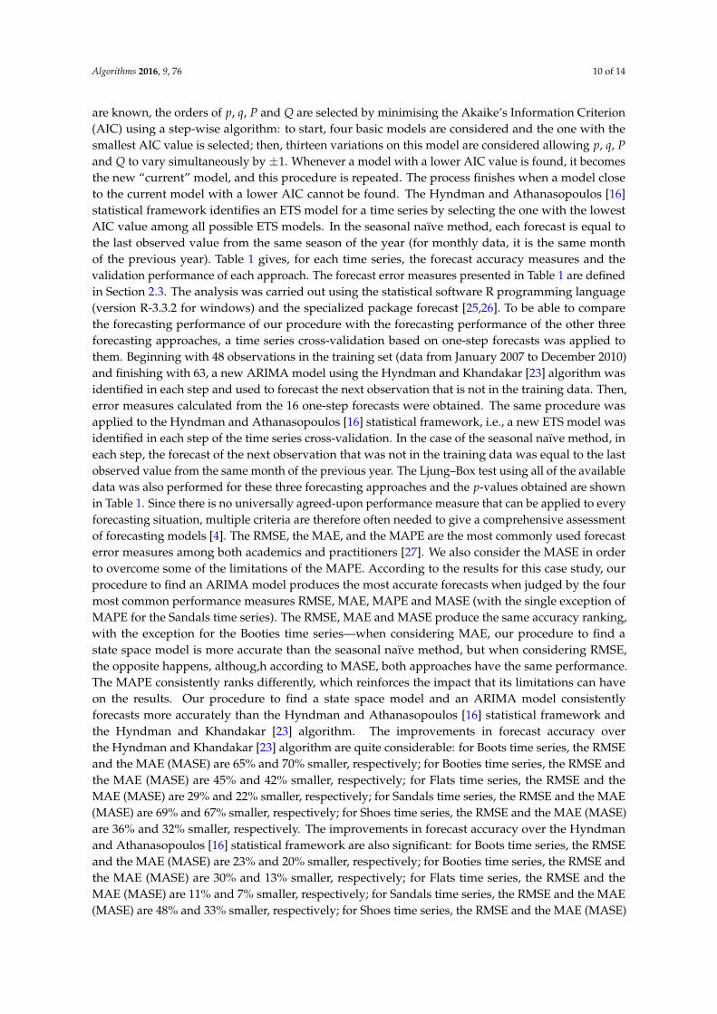
are known, the orders of p, q, P and Q are selected by minimising the Akaike’s Information Criterion(AIC) using a step-wise algorithm: to start, four basic models are considered and the one with thesmallest AIC value is selected; then, thirteen variations on this model are considered allowing p, q, Pand Q to vary simultaneously by ±1. Whenever a model with a lower AIC value is found, it becomesthe new “current” model, and this procedure is repeated. The process finishes when a model closeto the current model with a lower AIC cannot be found. The Hyndman and Athanasopoulos [16]statistical framework identifies an ETS model for a time series by selecting the one with the lowestAIC value among all possible ETS models. In the seasonal naïve method, each forecast is equal tothe last observed value from the same season of the year (for monthly data, it is the same monthof the previous year). Table 1 gives, for each time series, the forecast accuracy measures and thevalidation performance of each approach. The forecast error measures presented in Table 1 are definedin Section 2.3. The analysis was carried out using the statistical software R programming language(version R-3.3.2 for windows) and the specialized package forecast [25,26]. To be able to comparethe forecasting performance of our procedure with the forecasting performance of the other threeforecasting approaches, a time series cross-validation based on one-step forecasts was applied tothem. Beginning with 48 observations in the training set (data from January 2007 to December 2010)and finishing with 63, a new ARIMA model using the Hyndman and Khandakar [23] algorithm wasidentified in each step and used to forecast the next observation that is not in the training data. Then,error measures calculated from the 16 one-step forecasts were obtained. The same procedure wasapplied to the Hyndman and Athanasopoulos [16] statistical framework, i.e., a new ETS model wasidentified in each step of the time series cross-validation. In the case of the seasonal naïve method, ineach step, the forecast of the next observation that was not in the training data was equal to the lastobserved value from the same month of the previous year. The Ljung–Box test using all of the availabledata was also performed for these three forecasting approaches and the p-values obtained are shownin Table 1. Since there is no universally agreed-upon performance measure that can be applied to everyforecasting situation, multiple criteria are therefore often needed to give a comprehensive assessmentof forecasting models [4]. The RMSE, the MAE, and the MAPE are the most commonly used forecasterror measures among both academics and practitioners [27]. We also consider the MASE in orderto overcome some of the limitations of the MAPE. According to the results for this case study, ourprocedure to find an ARIMA model produces the most accurate forecasts when judged by the fourmost common performance measures RMSE, MAE, MAPE and MASE (with the single exception ofMAPE for the Sandals time series). The RMSE, MAE and MASE produce the same accuracy ranking,with the exception for the Booties time series—when considering MAE, our procedure to find astate space model is more accurate than the seasonal naïve method, but when considering RMSE,the opposite happens, althoug,h according to MASE, both approaches have the same performance.The MAPE consistently ranks differently, which reinforces the impact that its limitations can haveon the results. Our procedure to find a state space model and an ARIMA model consistentlyforecasts more accurately than the Hyndman and Athanasopoulos [16] statistical framework andthe Hyndman and Khandakar [23] algorithm. The improvements in forecast accuracy overthe Hyndman and Khandakar [23] algorithm are quite considerable: for Boots time series, the RMSEand the MAE (MASE) are 65% and 70% smaller, respectively; for Booties time series, the RMSE andthe MAE (MASE) are 45% and 42% smaller, respectively; for Flats time series, the RMSE and theMAE (MASE) are 29% and 22% smaller, respectively; for Sandals time series, the RMSE and the MAE(MASE) are 69% and 67% smaller, respectively; for Shoes time series, the RMSE and the MAE (MASE)are 36% and 32% smaller, respectively. The improvements in forecast accuracy over the Hyndmanand Athanasopoulos [16] statistical framework are also significant: for Boots time series, the RMSEand the MAE (MASE) are 23% and 20% smaller, respectively; for Booties time series, the RMSE andthe MAE (MASE) are 30% and 13% smaller, respectively; for Flats time series, the RMSE and theMAE (MASE) are 11% and 7% smaller, respectively; for Sandals time series, the RMSE and the MAE(MASE) are 48% and 33% smaller, respectively; for Shoes time series, the RMSE and the MAE (MASE)

Algorithms 2016, 9, 76 11 of 14

are 34% and 35% smaller, respectively. Our procedure to find an ARIMA model also outperformssignificantly the seasonal naïve method: for Boots time series, the RMSE and the MAE (MASE) are55% and 48% smaller, respectively; for Booties time series, the RMSE and the MAE (MASE) are 1%and 11% smaller, respectively; for Flats time series, the RMSE and the MAE (MASE) are 49% and51% smaller, respectively; for Sandals time series, the RMSE and the MAE (MASE) are 21% and 5%smaller, respectively; for Shoes time series, the RMSE and the MAE (MASE) are 52% and 60% smaller,respectively. In general, our procedure to find a state space model also forecasts more accuratelythan the seasonal seasonal naïve method: for Boots time series, the RMSE and the MAE (MASE) are11% and 4% smaller, respectively; for Booties time series, the RMSE is 15% larger, but the MAE is 1%smaller and the MASE is equal; for Flats time series, the RMSE and the MAE (MASE) are 47% and44% smaller, respectively; for Sandals time series, the RMSE and the MAE (MASE) are 19% and 47%larger, respectively; for Shoes time series, the RMSE and the MAE (MASE) are 49% and 56% smaller,respectively. The seasonal naïve model did not pass the Ljung–Box test in three of the five time seriesconsidering the usual significance level of 5%.

Table 1. Forecast accuracy measures of all forecasting approaches computed using time seriescross-validation.

Time Model RMSE Rank MAE Rank MAPE (%) Rank MASE Rank L-BSeries Test

Boots Log ARIMA(2, 1, 4)× (0, 0, 1)12 736.37 1 500.67 1 90.33 1 0.60 1 0.63ETS(M, A, A) 1470.95 2 921.14 2 206.71 4 1.11 2 0.05ETS Hyndman-Athanasopoulos (2013) framework 1918.63 4 1156.32 4 138.49 2 1.39 4 0.10ARIMA Hyndman-Khandakar (2008) algorithm 2104.56 5 1668.49 5 978.05 5 2.00 5 0.80Seasonal naïve method 1649.37 3 963.75 3 179.73 3 1.16 3 0.69

Booties Log ARIMA(3, 1, 3)× (1, 0, 0)12 406.53 1 284.43 1 61.54 1 0.72 1 0.66ETS(M, N, M) 480.83 3 319.66 2 73.25 4 0.81 2 0.10ETS Hyndman-Athanasopoulos (2013) framework 687.41 4 369.78 4 67.90 3 0.93 4 0.10ARIMA Hyndman-Khandakar (2008) algorithm 733.37 5 492.01 5 66.73 2 1.24 5 0.80Seasonal naïve method 409.57 2 321.44 3 149.30 5 0.81 2 0

Flats Log ARIMA(3, 0, 2)× (2, 1, 0)12 385.69 1 265.19 1 29.62 1 0.45 1 0.06ETS(M, Md, M) 401.61 2 299.30 2 31.32 3 0.51 2 0.55ETS Hyndman-Athanasopoulos (2013) framework 450.06 3 320.84 3 31.17 2 0.55 3 0.84ARIMA Hyndman-Khandakar (2008) algorithm 544.25 4 341.52 4 32.94 4 0.58 4 1.00Seasonal naïve method 750.80 5 536.44 5 47.62 5 0.92 5 0

Sandals ARIMA(1, 2, 2)× (0, 1, 2)12 1021.89 1 629.08 1 2217.84 4 0.55 1 0.05ETS(M, Ad, A) 1594.30 3 1259.59 3 7798.43 5 1.09 3 0.03ETS Hyndman-Athanasopoulos (2013) framework 3065.38 4 1866.34 4 270.90 2 1.62 4 0.07ARIMA Hyndman-Khandakar (2008) algorithm 3251.93 5 1921.29 5 591.37 3 1.67 5 0.41Seasonal naïve method 1287.04 2 670.00 2 101.78 1 0.58 2 0.44

Shoes Log ARIMA(0, 1, 0)× (1, 1, 2)12 607.29 1 443.88 1 12.84 1 0.35 1 0.11Log ETS(A, N, A) 643.73 2 481.06 2 13.76 2 0.38 2 0.54ETS Hyndman-Athanasopoulos (2013) framework 975.60 4 735.49 4 21.85 4 0.59 4 0.11ARIMA Hyndman-Khandakar (2008) algorithm 943.62 3 657.03 3 18.66 3 0.52 3 0.04Seasonal naïve method 1261.16 5 1096.5 5 34.79 5 0.88 5 0 1

1 p-value < 0.01.

Another observation that can be made from these results is that both transformation anddifferencing are important for improving ARIMA’s ability to model and forecast time series thatcontain strong trend and seasonal components. The log transformation was applied to four of thefive time series. With the exception of flats, all other time series were differenced: second-orderdifferences were made in Sandals series and first differences were made in Boots, Booties and Shoesseries. The Flats, Sandals and Shoes time series were seasonally differenced. Transformation seems notto be significant for state space models. Log transformation was made only on Shoes series.

To see the individual point forecasting behavior, the actual data versus the forecasts from allapproaches were plotted (see Figure 3). The ARIMA Cross-Validation and ETS Cross-Validationmodels selected by our procedure are identified in the legend by ARIMA_CV and ETS_CV, respectively.The forecasts from the Hyndman and Athanasopoulos [16] statistical framework are identified in thelegend by ETS_H-A. The forecasts from the Hyndman and Khandakar [23] algorithm are identifiedin the legend by ARIMA_H-K. In general, it can be seen that both ETS and ARIMA models selected

Algorithms 2016, 9, 76 12 of 14

by our cross-validation procedure have the capability to forecast the trend movement and seasonalfluctuations fairly well. As expected, the exceptional increase in the sales of flats observed in Marchand April 2012 was not predicted by the models that under-forecasted the situation. As mentioned inSection 2.3, one of the limitations of the MAPE is having huge values when data may contain verysmall numbers. The large values of MAPE for the Boots, Booties and Sandals time series are explainedby this fact, since, during some periods, there are almost no sales (close to zero).

(a)

Pai

rs o

f Boo

ts

(b)

Pai

rs o

f Boo

ties

(c)

Pai

rs o

f Fla

ts

(d)

Pai

rs o

f San

dals

Jan Feb Mar Apr May Jun Jul Aug Sep Oct Nov Dec Jan Feb Mar Apr

(e)

Pai

rs o

f Sho

es

Month

Data ARIMA_CV ETS_CV ETS_H−A ARIMA_H−K SNAIVE

Figure 3. One-step forecasts from all approaches computed using time series cross-validation (January2011 to April 2012): (a) pairs of Boots; (b) pairs of Booties; (c) pairs of Flats; (d) pairs of Sandals; and(e) pairs of Shoes.

Algorithms 2016, 9, 76 13 of 14

5. Conclusions

A common obstacle in using ARIMA models for forecasting is that the order selection processis usually considered subjective and difficult to apply. Identifying an appropriate state space modelfor a time series is also not an easy task. In this work, a cross-validation procedure is used to identifyan appropriate ARIMA model and an appropriate state space model for a time series. A minimumsize for the training set is specified. The procedure is based on one-step forecasts and uses differenttraining sets, each containing one more observation than the previous one. All possible ETS modelsand all ARIMA models where the orders are allowed to range reasonably are fitted considering rawdata and log-transformed data with regular differencing (up to second order differences) and, ifthe time series is seasonal, seasonal differencing (up to first order differences). The value of RMSEfor each model is calculated averaging the one-step forecasts obtained. The model which has thelowest RMSE value and passes the Ljung–Box test using all of the available data with a reasonablesignificance level is selected among all the ARIMA and ETS models considered. One of the advantagesof this model identification procedure is to be able to compare models that have different ordersof differencing and/or different transformations, which is not the case when models are comparedusing Akaike’s Information Criterion or Bayesian Information Criterion values. The application of themodel identification procedure is exemplified in the paper with a case study of retail sales of differentcategories of women’s footwear from a Portuguese retailer. To be able to compare the accuracies ofthe forecasts obtained with the ETS and ARIMA models selected by the cross-validation proceduredeveloped, we also evaluated the forecasts from another three forecasting approaches: the Hyndmanand Khandakar [23] algorithm for ARIMA models, the Hyndman and Athanasopoulos [16] statisticalframework for ETS models and the seasonal naïve method. According to the results, our procedure tofind an ARIMA model produces the most accurate forecasts when judged by RMSE, MAE, MAPE andMASE. The RMSE, MAE and MASE produce the same accuracy ranking. The MAPE consistently ranksdifferently, which reinforces the impact that its limitations can have on the results. Our procedureto find a state space model and an ARIMA model consistently forecasts more accurately than theHyndman and Athanasopoulos [16] statistical framework and the Hyndman and Khandakar [23]algorithm, and the improvements in the forecast accuracy are significant. Both transformation anddifferencing were important for improving ARIMA’s ability to model. Transformation did not seemto be significant for accuracy for state space models. Large values of MAPE were found when datacontained numbers close to zero, which shows the effect that the limitations of this accuracy measuremay have on forecasting results.

Acknowledgments: Project "TEC4Growth-Pervasive Intelligence, Enhancers and Proofs of Concept withIndustrial Impact/NORTE-01-0145-FEDER-000020" is financed by the North Portugal Regional OperationalProgramme (NORTE 2020), under the PORTUGAL 2020 Partnership Agreement, and through the EuropeanRegional Development Fund (ERDF).

Author Contributions: Patrícia Ramos designed the cross-validation procedure and José Manuel Oliveiraimplemented the algorithm and performed the empirical study. Patrícia Ramos wrote the paper andJosé Manuel Oliveira helped to improve the manuscript. Both authors read and approved the final manuscript.

Conflicts of Interest: The authors declare no conflict of interest.

References

1. Alon, I. Forecasting aggregate retail sales: The Winters’ model revisited. In Proceedings of the 1997 MidwestDecision Science Institute Annual Conference, Indianapolis, IN, USA, 24–26 April 1997; pp. 234–236.

2. Alon, I.; Min, Q.; Sadowski, R.J. Forecasting aggregate retail sales: A comparison of artificial neural networksand traditional method. J. Retail. Consum. Serv. 2001, 8, 147–156.

3. Frank, C.; Garg, A.; Sztandera, L.; Raheja, A. Forecasting women’s apparel sales using mathematicalmodeling. Int. J. Cloth. Sci. Technol. 2003, 15, 107–125.

4. Chu, C.W.; Zhang, P.G.Q. A comparative study of linear and nonlinear models for aggregate retail salesforecasting. Int. J. Prod. Econ. 2003, 86, 217–231.

Algorithms 2016, 9, 76 14 of 14

5. Aburto, L.; Weber, R. Improved supply chain management based on hybrid demand forecasts. Appl. SoftComput. 2007, 7, 126–144.

6. Zhang, G.; Qi, M. Neural network forecasting for seasonal and trend time series. Eur. J. Oper. Res. 2005,160, 501–514.

7. Kuvulmaz, J.; Usanmaz, S.; Engin, S.N. Time-series forecasting by means of linear and nonlinear models.In Advances in Artificial Intelligence; Springer: Berlin/Heidelberg, Germany, 2005.

8. Box, G.; Jenkins, G.; Reinsel, G. Time Series Analysis, 4th ed.; Wiley: Hoboken, NJ, USA, 2008.9. Hyndman, R.J.; Koehler, A.B.; Ord, J.K.; Snyder, R.D. Forecasting with Exponential Smoothing: The State Space

Approach; Springer: Berlin, Germany, 2008.10. Pena, D.; Tiao, G.C.; Tsay, R.S. A Course in Time Series Analysis; John Wiley & Sons: New York, NY, USA, 2001.11. Zhao, X.; Xie, J.; Lau, R.S.M. Improving the supply chain performance: Use of forecasting models versus

early order commitments. Int. J. Prod. Res. 2001, 39, 3923–3939.12. Gardner, E.S. Exponential smoothing: The state of the art. J. Forecast. 1985, 4, 1–28.13. Makridakis, S.; Wheelwright, S.; Hyndman, R. Forecasting: Methods and Applications, 3rd ed.; John Wiley & Sons:

New York, NY, USA, 1998.14. Gardner, E.S. Exponential smoothing: The state of the art-Part II. Int. J. Forecast. 2006, 22, 637–666.15. Aoki, M. State Space Modeling of Time Series; Springer: Berlin, Germany, 1987.16. Hyndman, R.J.; Athanasopoulos, G. Forecasting: Principles and Practice; OTexts: Melbourne, Australia, 2013.17. Ljung, G.M.; Box, G.E.P. On a measure of lack of fit in time series models. Biometrika 1978, 65, 297–303.18. Brockwell, P.J.; Davis, R.A. Introduction to Time Series and Forecasting, 2nd ed; Springer: New York, NY,

USA, 2002.19. Shumway, R.H.; Stoffer, D.S. Time Series Analysis and Its Applications: With R Examples, 3rd ed; Springer:

New York, NY, USA, 2011.20. Wei, W.S. Time Series Analysis: Univariate and Multivariate Methods, 2nd ed; Addison Wesley: Boston, MA,

USA, 2005.21. Hyndman, R.J.; Koehler, A.B. Another look at measures of forecast accuracy. Int. J. Forecast. 2006, 22, 679–688.22. Arlot, S.; Alain, C. A survey of cross-validation procedures for model selection. Stat. Surv. 2010, 4, 40–79.23. Hyndman, R.J.; Khandakar, Y. Automatic time series forecasting: the forecast package for R. J. Stat. Softw.

2008, 27, 1–22.24. Kwiatkowski, D.; Phillips, P.C.; Schmidt, P.; Shin, Y. Testing the null hypothesis of stationariry against the

alternative of a unit root. J. Econom. 1992, 54, 159–178.25. R Core Team. R: A Language and Environment for Statistical Computing; R Foundation for Statistical Computing:

Vienna, Austria, 2016.26. Hyndman, R.J. Forecast: Forecasting Functions for Time Series and Linear Models. R package Version 7.3.

Available online: http://github.com/robjhyndman/forecast (accessed on 7 November 2016).27. Fildes, R.A.; Goodwin, P. Against your better judgment? How organizations can improve their use of

management judgment in forecasting. Interfaces 2007, 37, 570–576.

c© 2016 by the authors; licensee MDPI, Basel, Switzerland. This article is an open accessarticle distributed under the terms and conditions of the Creative Commons Attribution(CC-BY) license (http://creativecommons.org/licenses/by/4.0/).