a prototype high resolution 3d radar reflectivity mosaic ... · a prototype high resolution 3d...

ERAD 2014 - THE EIGHTH EUROPEAN CONFERENCE ON RADAR IN METEOROLOGY AND HYDROLOGY

A Prototype High Resolution 3D Radar Reflectivity Mosaic forSESAR

Robert Scovell1, Hassan al-Sakka2, Nicolas Gaussiat2, and Pierre Tabary2

1Met Office, Fitzroy Road, EX1 3PB Exeter, UK.2Météo-France, 42 Rue Gaspard Coriolis, 31057 Toulouse, France.

(Dated: 12th November 2014)

1. Introduction

The Single European Skies Air Traffic Management Research (SESAR) programme is an international partnership, foundedby Eurocontrol and EUMETNET, which aims to deliver the next generation European air traffic management system, with EU-wide deployment due by the end of this decade. As part of this effort, SESAR has defined a work package specifically for themeterological systems infrastructure: WP 11.2.2.: MET Systems Development, Verification and Validation. The deliverablesinclude the provision of a 3D radar reflectivity mosaic and a suite of related 2D column-integrated products derived fromthe operational network of European radars and focussing on the Terminal Manoeuvering Areas (TMAs) surrounding majorairports. Work started on these radar-specific deliverables in Spring 2013 as a collaborative project between Météo-France andthe UK Met Office. Progress made to date is reported in this abstract.

The idea to combine reflectivity data from multiple radars on to a 3D grid has been studied for some time, see for examplesee Bousquet and Chong (1998) or Zhang et al. (2005). In an operational context, the production of such 3D products can posea technical challenge due to the short lead times required and the large volumes of data involved (both in terms of RandomAccess Memory (RAM) and CPU time needed to carry out the processing).

Zhang et al. (2011) describe the U.S. CONUS (Contiguous U.S.) reflectivity mosaic, which is part of their National Multi-Sensor QPE (NMQ) system. This system first performs interpolation (polar to Cartesian transformation) for each radar PlanPosition Indicator (PPI) scan separately resulting in a single-radar Cartesian 3D grid ( which is itself a sub-grid of the multi-radar 3D mosaic, extending over the CONUS domain ). Single radar grids are then combined on the domain-wide grid using aweighted average, where the weighting of each radar is dependent on the distance of the 3D radar grid cell from the radar site(also known as Distance Weighted Mean (DWM)), with lower weights assigned to grid cells which are further away.

A similar approach was taken by Bousquet and Chong (1998) as part of the Multiple Doppler Synthesis and ContinuityAdjustment Technique (MUSCAT), which was primarily designed for retrieval of 3D Doppler winds. This algorithm was usedto create a low resolution (2.5km,15 min.) 3D Doppler and reflectivity product, covering the whole of France, called 3DNat,and was made operational at Météo France in 2009 by Kergomard et al. after a successful evaluation over the Greater Parisregion (Bousquet et al., 2008).

In this project we have studied two prototype methods for 3D reflectivity retrieval. The first is an enhanced version of the3DNat method (called FRM) which is now capable of running at the required 1km horizontal, 500m vertical and 5 minutetemporal resolution. Secondly a new method (called UKM) has been developed which skips the intermediate single-radar gridsand produces mosaics directly at the required resolution from the PPI data. These methods are described later in this abstract.

ERAD 2014 Abstract ID 141 1 [email protected]


2. Specification of prototype

2.1. 3D mosaic domains

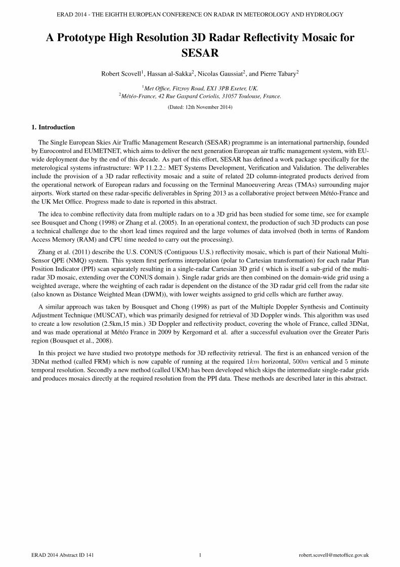
Figure 1: Yellow: LHR and CDG prototype domains, Orange: 100km coverage of UK radars, Red: 100km coverage of Jerseyradar, Blue: 100km coverage of French radars

The prototype system includes two domains (see Fig.1); one enclosing the Terminal Manoeuvering Area (TMA) of HeathrowAirport in London (LHR) and the other including the TMA of Charles de Gaulle Airport in Paris (CDG). They are defined inthe Polar Stereographic map projection (Snyder, 1987) but with the latitude of the true scale shifted from the North Pole to theairports (to avoid scale distortions) and they extend horizontally by 400km x 400km at 1km resolution with a vertical ceilingof 12km (≈ 40000ft) and 500m vertical level spacing. The choice of vertical extent is motivated by the fact that nearly allcivil aircraft fly below this altitude and at the latitudes of Paris and London, it is rare for convective cells to exceed this height.A 5 minute temporal resolution is being used and it is anticipated that the products will become available with lead times lessthan 5 minutes after data time.

2.2. 2D and 3D products

The prototype products include a 3D gridded reflectivity product (in dB units) which is defined at all grid points within the3dB beamwidth of the radar scans forming the network. Directly from this grid, using the data available in the vertical columnabove each horizontal grid point, a suite of 2D column-integrated products (see Table 1) are derived. These give useful insightsinto the structure of the 3D reflectivity and also are good indicators of the severity of convective storm developments.

Name Description UnitsETOP18 18 dBZ echo top height mETOP45 45 dBZ echo top height mZMAX Column-maximum reflectivity dB

ALTZMAX Height of maximum reflectivity in the column mVIL Vertically Integrated Liquid kgm−2

Table 1: 2D product types.

Reasonable estimates of ETOP and (ALT)ZMAX are gained by direct extraction from the 3D gridded reflectivity, while the

ERAD 2014 Abstract ID 141 2


VIL is calculated by integrating the reflectivity over all height levels using the method of Greene and Clark (1972). Figure 2shows examples of the 2D products for a convective supercell storm that was seen on 28th June 2012 in the Midlands regionof England.

2.3. Coverage

The UK radar network includes 16 C-band radars (including one owned by the Jersey Met Department) and Météo-Francemaintain 27 S,C and X band radars (although only the C-band radars overlap with the prototype domain). The radars that arerelevant to the LHR and CDG domains are shown in Figure 1 and some relevant characteristics of these radars are listed inTable 2.

Quantity Météo-France UK Met Office (inc. Jersey)3dB beamwidth (◦) 1.1 1.1

Range gate spacing (km) 1.0 0.6Maximum range (km) 256.0 255.0

Table 2: Characteristics of UK and French radars.

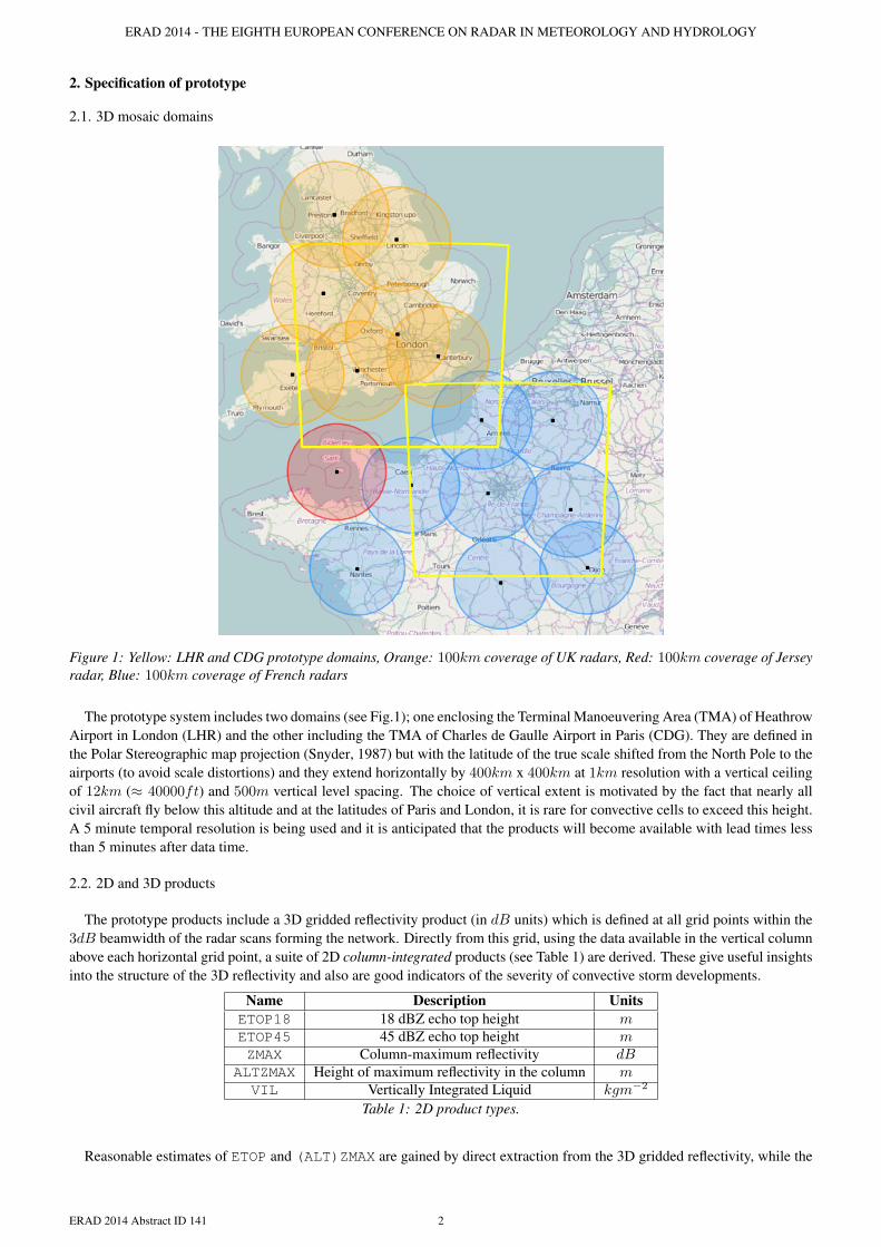
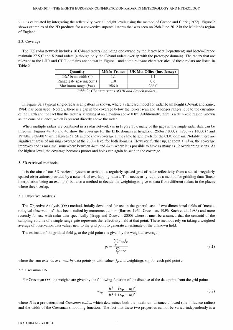
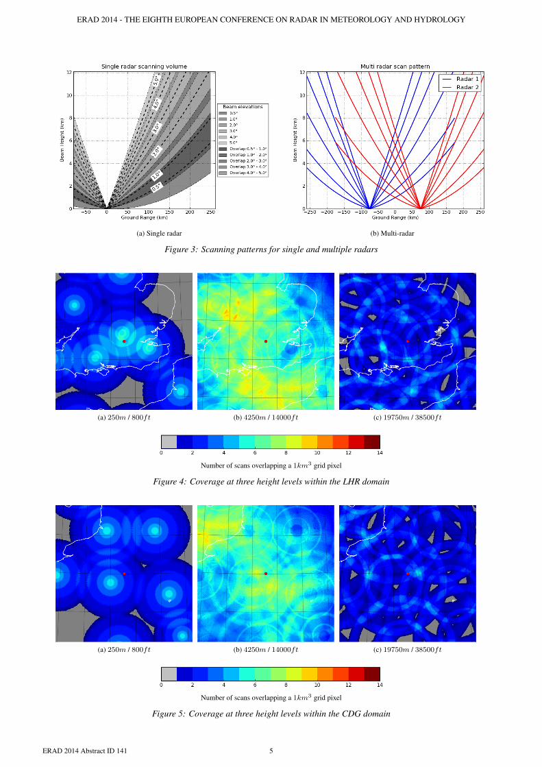
In Figure 3a a typical single-radar scan pattern is shown, where a standard model for radar beam height (Doviak and Zrnic,1984) has been used. Notably, there is a gap in the coverage below the lowest scan and at longer ranges, due to the curvatureof the Earth and the fact that the radar is scanning at an elevation above 0.0◦. Additionally, there is a data-void region, knownas the cone of silence, which is present directly above the radar.

When multiple radars are combined in a radar network (as in Figure 3b), many of the gaps in the single radar data can befilled-in. Figures 4a, 4b and 4c show the coverage for the LHR domain at heights of 250m / 800ft, 4250m / 14000ft and19750m / 38500ft while figures 5a, 5b and 5c show coverage at the same height levels for the CDG domain. Notably, there aresignificant areas of missing coverage at the 250m level for both domains. However, further up, at about ≈ 4km, the coverageimproves and is maximal somewhere between 4km and 5km where it is possible to have as many as 12 overlapping scans. Atthe highest level, the coverage becomes poorer and holes can again be seen in the coverage.

3. 3D retrieval methods

It is the aim of our 3D retrieval system to arrive at a regularly spaced grid of radar reflectivity from a set of irregularlyspaced observations provided by a network of overlapping radars. This necessarily requires a method for gridding data (linearinterpolation being an example) but also a method to decide the weighting to give to data from different radars in the placeswhere they overlap.

3.1. Objective Analysis

The Objective Analysis (OA) method, intially developed for use in the general case of two dimensional fields of "meteo-rological observations", has been studied by numerous authors (Barnes, 1964; Cressman, 1959; Koch et al., 1983) and morerecently for use with radar data specifically (Trapp and Doswell, 2000) where it must be assumed that the centroid of thesampling volume of a single range gate represents the reflectivity field at that point. These methods rely on taking a weightedaverage of observation data values near to the grid point to generate an estimate of the unknown field.

The estimate of the gridded field gi at the grid point i is given by the weighted average:

gi =

∑pwipfp∑pwip

(3.1)

where the sum extends over nearby data points p, with values fp and weightings wip for each grid point i.

3.2. Cressman OA

For Cressman OA, the weights are given by the following function of the distance of the data point from the grid point:

wip =R2 − (xp − xi)

2

R2 + (xp − xi)2 (3.2)

where R is a pre-determined Cressman radius which determines both the maximum distance allowed (the influence radius)and the width of the Cressman smoothing function. The fact that these two properties cannot be varied independently is a



(a) 18 dBZ echo top (b) 45 dBZ echo top

(c) Max. dBZ (d) Alt. dBZ-max

(e) VIL

Figure 2: 2D column-integrated products for a 80km × 80km × 12km test domain in the Midlands, England on 28th June2012 13:00:00 UTCERAD 2014 Abstract ID 141 4


(a) Single radar (b) Multi-radar

Figure 3: Scanning patterns for single and multiple radars

(a) 250m / 800ft (b) 4250m / 14000ft (c) 19750m / 38500ft

Number of scans overlapping a 1km3 grid pixel

Figure 4: Coverage at three height levels within the LHR domain

(a) 250m / 800ft (b) 4250m / 14000ft (c) 19750m / 38500ft

Number of scans overlapping a 1km3 grid pixel

Figure 5: Coverage at three height levels within the CDG domain



limitation of the Cressman approach.

3.3. Barnes OA

In Barnes OA, the weighting is a Gaussian function of the distance of the data point from the grid point:

wip = e−(xp−xi)2/κ (3.3)

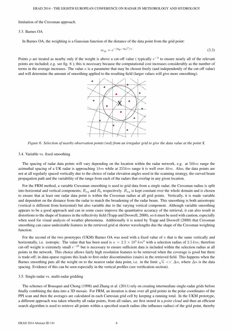
Points p are treated as nearby only if the weight is above a cut-off value ( typically e−3 to ensure nearly all of the relevantpoints are included; e.g. see fig. 6 ); this is necessary because the computational cost increases considerably as the number ofterms in the average increases. The value κ is a parameter that may be chosen freely (and independently of the cut-off value)and will determine the amount of smoothing applied to the resulting field (larger values will give more smoothing).

Figure 6: Selection of nearby observation points (red) from an irregular grid to give the data value at the point X.

3.4. Variable vs. fixed smoothing

The spacing of radar data points will vary depending on the location within the radar network, e.g. at 50km range theazimuthal spacing of a UK radar is approaching 1km while at 255km range it is well over 4km. Also, the data points arenot at all regularly spaced vertically due to the choice of radar elevation angles used in the scanning strategy, the curved beampropagation path and the variability of the range from each of the radars that overlap in any given location.

For the FRM method, a variable Cressman smoothing is used to grid data from a single radar; the Cressman radius is splitinto horizontal and vertical components; Rxy and Rh respectively. Rxy is kept constant over the whole domain and is chosento ensure that at least one radar data point is within the Cressman radius at all grid points. Vertically, it is made variableand dependent on the distance from the radar to match the broadening of the radar beam. This smoothing is both anisotropic(vertical is different from horizontal) but also variable due to the varying vertical component. Although variable smoothingappears to be a good approach and can in some cases improve the quantitative accuracy of the retrieval, it can also result indistortions to the shape of features in the reflectivity field (Trapp and Doswell, 2000), so it must be used with caution, especiallywhen used for visual analysis of weather phenomena. Additionally it is noted by Trapp and Doswell (2000) that Cressmansmoothing can cause undesirable features in the retrieved grid at shorter wavelengths due the shape of the Cressman weightingfunction.

For the second of the two prototypes (UKM) Barnes OA was used with a fixed value of κ that is the same vertically andhorizontally, i.e. isotropic. The value that has been used is κ = 2.5 × 105 km2 with a selection radius of 2.5 km; thereforecut-off weight is extremely small e−25 but is necessary to ensure sufficient data is included within the selection radius at allpoints in the network. This choice allows fairly high resolution features to be retrieved when the coverage is good but thereis trade-off; in data-sparse regions this leads to first-order discontinuities (stairs) in the retrieved field. This happens when theBarnes smoothing puts all the weight on to the nearest radar data point, i.e. in the limit

√κ << ∆n, where ∆n is the data

spacing. Evidence of this can be seen especially in the vertical profiles (see verification section).

3.5. Single-radar vs. multi-radar gridding

The schemes of Bousquet and Chong (1998) and Zhang et al. (2011) rely on creating intermediate single-radar grids beforefinally combining the data into a 3D mosaic. For FRM, an iteration is done over all grid points in the polar coordinates of thePPI scan and then the averages are calculated in each Cartesian grid cell by keeping a running total. In the UKM prototype,a different approach was taken whereby all radar points, from all radars, are first stored in a point cloud and then an efficientsearch algorithm is used to retrieve all points within a specified search radius (the influence radius) of the grid point, thereby



allowing data points from all radars to be considered together for the purposes of creating the 3D Cartesian grid value. Thetwo approaches are shown in Figure 7.

(a) With intermediate grid (b) Without intermediate grid

Figure 7: 3D mosaic strategies with and without intermediate grids

This alternative approach was motivated by the desire to have more flexibility when combining data from multiple radars.Additionally, this allows 2D products (such as maximum reflectivity) to be extracted directly from the original radar datavalues. This has not been fully investigated and, at present, the UKM prototype uses the same method as FRM, i.e. it retrievesthe 2D fields from the 3D gridded reflectivity.

3.6. Multi-radar mosaic and Distance Weighted Mean

The FRM method and also Zhang et al. (2011) use a Distance Weighted Mean (DWM) to combine data from multiple radarsafter they have already been put on to Cartesian grids. For FRM, the weighting takes a Gaussian form, for radar l which is atrange rl,ijk from grid point ijk:

wl = e−r2

l,ijkK (3.4)

so that at longer ranges the weighting is lower. A tunable parameter K controls the relative weighting given to pixels atdifferent ranges and may be thought of as an estimate of the radar pixel quality degredation due to beam broadening with range(the exponent may be written in terms of the radar beam width, rφ, if K ∝ 1

φ2 ). A value of K was chosen by eye for FRM inorder to optimise the retrieved reflectivity field.

Initially for UKM, it was decided to use a similar factor but to introduce it directly into the OA weighted average. However,it was later omitted because it was discovered that the resulting retrieved reflectivity fields were relatively insensitive to it (asexplained in the final section).

3.7. Alternatives to OA

An alternative approach to the established OA + DWM based on an inverse method to retrieve 3D radar reflectivity has beenhighlighted recently (Roca-Sancho et al., 2014; Yang et al., 2011). This is promising because it appears to offer a means toproperly take into account the radar sampling when data from multiple radars overlap, rather than making the approximationthat the radar data value is represented by a discrete point in space. It has not been possible to study this method within thescope of this project, given that this is a very recent development.

4. Verification

Two approaches have been used to determine the accuracy of the retrieved 3D gridded reflectivity. The first is to remove aradar from the network and then compare a retrieval based on the network of remaining radars to this data from the removedradar only. Secondly, the radar PPIs have been simulated based on a known 3D field and then the results of a retrieval fromthese PPIs are compared to the original field. The results of the verification are given in more detail in a paper by al Sakkaet al. (2014) at this conference but the second method is summarized briefly here.

4.1. Simulation of a radar network

Figure 8a shows idealised Vertical Profiles of Reflectivity for both convective and stratiform cases. It is possible to createsynthetic 3D radar reflectivity fields (Figure 8b), one for each profile, over the LHR and CDG domains, by assigning to eachgrid pixel the value of the chosen profile at the height of that pixel (this results in a horizontally homogenious 3D field). Theradar sampling of these fields is then simulated, for each range gate in a PPI scan, by integrating the synthetic reflectivity fieldover the sampling volume weighted by the radar beam power (using the standard expression for the received power; see Doviakand Zrnic (1984), p. 52).



(a) Right (b) Left

Figure 8: Idealized VPRs and Y-Z cross sections of synthetic 3D reflectivity fields.

(a) Stratiform, FRM (b) Convective, FRM

(c) Stratiform, UKM (d) Convective, UKM

Figure 9: Y-Z cross sections of 3D fields retrieved from simulated PPI network over LHR domain



Figure 10: 25 profiles from the retrieved grid (UKM and FRM methods) over the CDG domain

Using the simulated PPIs, it is possible to build up a simulated radar network which can subsequently can be fed-in to the3D radar reflectivity retrieval algorithm (UKM or FRM).

4.2. Results of simulation

Y-Z cross-sections for LHR domain retrievals using both FRM and UKM are shown in Figure 9 while Figure 10 shows theprofiles at 25 locations within the CDG domain (with ≈ 80 km spacing), for both UKM and FRM, alongside the idealizedprofile. It can be seen that there is better agreement to the reference with the UKM, compared to the FRM, but there existnoticable first-order discontinuities (stairs) in some of the profiles. As mentioned earlier, this "stairs" effect is due to therelatively small smoothing parameter κ compared to the data spacing, in data sparse regions.

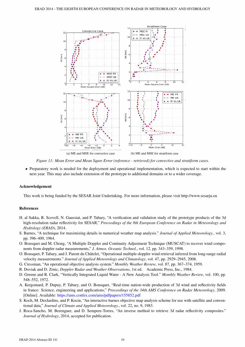
Figures 11a and 11b show the mean error (or bias) and the mean square error at each height level, averaged over 121 verticalprofiles (with ≈ 40 km spacing) within the CDG domain, for both the convective and stratiform cases. It can be seen that theUKM performs better generally in terms of these quantitative measures, except in a few places. The greatest errors in bothUKM and FRM appear when there are the strongest gradients in the idealized profile.

It is believed that the reason the UKM performs well, without using the DWM, is because it naturally weights radars whichare nearer to the grid pixel being considered. This is due to the fact that the density of the radar range gates in radar volume isgreater at shorter ranges, hence there are more pixels from those radars in the search radius.

5. Current and future work

• Temporal synchronization of PPI scans is needed to ensure that the meteorological features in the radar data as seen bydifferent radars appear in the same place. The intention is to determine the motion vectors using Optical Flow, allowingadvection of radar data points before OA.

• A beam blockage correction needed, especially at lower elevations. Work has been done to correct for this and will beimplemented in the next release of the prototype.

• Further verification work will be done, including an extension of the synthetic reflectivity field to include horizontalvariability.

• It is the intention to make use of radar pixel quality measures to allow data to be given a small weighting when it isknown that the radar is performing poorly.

• The final choice for the 3D mosaic method that will become operational needs to be decided, along with some furtherrefinements to tune the OA such at the errors are minimized. This may include extending the UKM to a multi-pass OAmethod, as is done in the original methods of Barnes (1964) and Cressman (1959).



(a) ME and MSE for convective case (b) ME and MSE for stratiform case

Figure 11: Mean Error and Mean Squre Error (reference - retrieved) for convective and stratiform cases.

• Preparatory work is needed for the deployment and operational implementation, which is expected to start within thenext year. This may also include extension of the prototype to additional domains or to a wider coverage.

Acknowledgement

This work is being funded by the SESAR Joint Undertaking. For more information, please visit http://www.sesarju.eu

References

H. al Sakka, R. Scovell, N. Gaussiat, and P. Tabary, “A verification and validation study of the prototype products of the 3dhigh-resolution radar reflectivity for SESAR,” Proceedings of the 8th European Conference on Radar in Meteorology andHydrology (ERAD), 2014.

S. Barnes, “A technique for maximizing details in numerical weather map analysis.” Journal of Applied Meteorology., vol. 3,pp. 396–409, 1964.

O. Bousquet and M. Chong, “A Multiple Doppler and Continuity Adjustment Technique (MUSCAT) to recover wind compo-nents from doppler radar measurements,” J. Atmos. Oceanic Technol., vol. 12, pp. 343–359, 1998.

O. Bousquet, P. Tabary, and J. Parent du Châtelet, “Operational multiple-doppler wind retrieval inferred from long-range radialvelocity measurements.” Journal of Applied Meteorology and Climatology, vol. 47, pp. 2929–2945, 2008.

G. Cressman, “An operational objective analysis system.” Monthly Weather Review, vol. 87, pp. 367–374, 1959.R. Doviak and D. Zrnic, Doppler Radar and Weather Observations, 1st ed. Academic Press, Inc., 1984.D. Greene and R. Clark, “Vertically Integrated Liquid Water - A New Analysis Tool.” Monthly Weather Review, vol. 100, pp.

548–552, 1972.A. Kergomard, P. Dupuy, P. Tabary, and O. Bousquet, “Real-time nation-wide production of 3d wind and reflectivity fields

in france: Science, engineering and applications,” Proceedings of the 34th AMS Conference on Radar Meteorology, 2009.[Online]. Available: https://ams.confex.com/ams/pdfpapers/155852.pdf

S. Koch, M. DesJardins, and P. Kocin, “An interactive barnes objective map analysis scheme for use with satellite and conven-tional data,” Journal of Climate and Applied Meteorology., vol. 22, no. 9, 1983.

J. Roca-Sancho, M. Berenguer, and D. Sempere-Torres, “An inverse method to retrieve 3d radar reflectivity composites.”Journal of Hydrology, 2014, accepted for publication.


https://ams.confex.com/ams/pdfpapers/155852.pdf


J. Snyder, “Map projections: A working manual,” USGS Professional Paper: 1395, 1987. [Online]. Available:http://pubs.er.usgs.gov/publication/pp1395

R. Trapp and C. Doswell, “Radar data objective analysis.” Journal of Atmospheric and Oceanic Technology, vol. 17, pp.105–120, 2000.

Y. Yang, D. Chen, L. Gan, and F. Y., “Three-dimensional gridding and mosaic of reflectivities frommultiple radars with a two-step variational method.” Proceedings of the 2011 International Conference on Re-mote Sensing, Environment and Transportation Engineering (RSETE)., pp. 2778–2781, 2011. [Online]. Avail-able: http://www.researchgate.net/publication/236315116_Three-dimensional_gridding_and_mosaic_of_reflectivities_from_multiple_radars_with_a_two-step_variational_method

J. Zhang, K. Howard, and J. Gourley, “Constructing three-dimensional multiple-radar reflectivity mosaics: Examples of con-vective storms and stratiform rain echoes,” Journal of Atmospheric and Oceanic Technology, vol. 22, pp. 30–42, 2005.

J. Zhang, K. Howard, C. Langston, S. Vasiloff, B. Kaney, A. Arthur, S. Van Cooten, K. Kelleher, D. Kitzmiller, F. Ding,D. Seo, E. Wells, and C. Dempsey, “National Mosaic and Multi-sensor QPE (nmq) System.” Bull. Amer. Met. Soc., vol. 92,pp. 1321–1338, 2011.


http://pubs.er.usgs.gov/publication/pp1395

http://www.researchgate.net/publication/236315116_Three-dimensional_gridding_and_mosaic_of_reflectivities_from_multiple_radars_with_a_two-step_variational_method

http://www.researchgate.net/publication/236315116_Three-dimensional_gridding_and_mosaic_of_reflectivities_from_multiple_radars_with_a_two-step_variational_method

a prototype high resolution 3d radar reflectivity mosaic ... · a prototype high resolution 3d...

Documents