a pure-jump market-making model for high-frequency trading
TRANSCRIPT

Purdue UniversityPurdue e-Pubs
Open Access Dissertations Theses and Dissertations
Spring 2015
A pure-jump market-making model for high-frequency tradingChi Wai LawPurdue University
Follow this and additional works at: https://docs.lib.purdue.edu/open_access_dissertations
Part of the Finance and Financial Management Commons, Mathematics Commons, and theStatistics and Probability Commons
This document has been made available through Purdue e-Pubs, a service of the Purdue University Libraries. Please contact [email protected] foradditional information.
Recommended CitationLaw, Chi Wai, "A pure-jump market-making model for high-frequency trading" (2015). Open Access Dissertations. 496.https://docs.lib.purdue.edu/open_access_dissertations/496

Graduate School Form 30Updated 1/15/2015
PURDUE UNIVERSITYGRADUATE SCHOOL
Thesis/Dissertation Acceptance
This is to certify that the thesis/dissertation prepared
By
Entitled
For the degree of
Is approved by the final examining committee:
To the best of my knowledge and as understood by the student in the Thesis/Dissertation Agreement, Publication Delay, and Certification Disclaimer (Graduate School Form 32), this thesis/dissertation adheres to the provisions of Purdue University’s “Policy of Integrity in Research” and the use of copyright material.
Approved by Major Professor(s):
Approved by: Head of the Departmental Graduate Program Date
Chi Wai Law
A Pure-Jump Market-Making Model for High-Frequency Trading
Doctor of Philosophy
Frederi G. ViensChair
Fabrice Baudoin
Hao Zhang
Jose E. Figueroa-Lopez
Frederi Viens
Jun Xie 4/21/2015


A PURE-JUMP MARKET-MAKING MODEL
FOR HIGH-FREQUENCY TRADING
A Dissertation
Submitted to the Faculty
of
Purdue University
by
Chi Wai Law
In Partial Fulfillment of the
Requirements for the Degree
of
Doctor of Philosophy
May 2015
Purdue University
West Lafayette, Indiana

ii
Dedicated to my parents
Tat Hung Law & Kit Chun Li
and siblings
Dikman Law & Anthea Law

iii
ACKNOWLEDGMENTS
This thesis could not have been completed without the tremendous help from my advi-
sor Prof. Frederi G. Viens, who has been my mentor since day one when I came to Purdue.
I am indebted to his enthusiastic support, guidance and encouragement throughout the four
years of my PhD study. Under the enjoyable supervision of Prof. Viens, I have the freedom
to discover my niche without the burden of following any prescribed route. Theoretical
research is elegant, refined and polished but I also adore the powerful impact that applied
research can create. However, without the profound knowledge of Prof. Viens, I could
have fallen into the trap of endless exploration before settling down to a realistic agenda.
High-frequency algorithmic trading is a new topic that has so many exciting areas and I am
so delighted to have had the opportunity to work with Prof. Viens on this subject.
I would also like to thank my committee, Prof. Hao Zhang, Prof. Jose E. Figueroa-
Lopez and Prof. Fabrice Baudoin, for their inspiration, backing as well as challenging
questions, in addition to our beloved Department Head Prof. Rebecca W. Doerge, and
Graduate Chair Prof. Jun Xie, for their unlimited counseling during my academic journey.
Finally, I would give my full appreciation to the love and consideration from my par-
ents, who always stand by me to navigate through difficult times. Without their countless
sacrifices, I would not have been able to fulfil my dream.

iv
TABLE OF CONTENTS
Page
LIST OF TABLES . . . . . . . . . . . . . . . . . . . . . . . . . . . . . . . . . vii
LIST OF FIGURES . . . . . . . . . . . . . . . . . . . . . . . . . . . . . . . . viii
SYMBOLS . . . . . . . . . . . . . . . . . . . . . . . . . . . . . . . . . . . . ix
ABBREVIATIONS . . . . . . . . . . . . . . . . . . . . . . . . . . . . . . . . x
ABSTRACT . . . . . . . . . . . . . . . . . . . . . . . . . . . . . . . . . . . . xi
1 Introduction . . . . . . . . . . . . . . . . . . . . . . . . . . . . . . . . . . 11.1 Background . . . . . . . . . . . . . . . . . . . . . . . . . . . . . . . 11.2 Review of Market-Making Models . . . . . . . . . . . . . . . . . . . . 2
1.2.1 Garman (1976) . . . . . . . . . . . . . . . . . . . . . . . . . . 31.2.2 Ho and Stoll (1981) . . . . . . . . . . . . . . . . . . . . . . . 41.2.3 Avellaneda and Stoikov (2008) . . . . . . . . . . . . . . . . . . 41.2.4 Guilbaud and Pham (2013) . . . . . . . . . . . . . . . . . . . . 5
1.3 Issues of Existing Market-Making Models . . . . . . . . . . . . . . . . 5
2 A New Pure-Jump Market-Making Model for High-Frequency Trading . . . . 72.1 Prices and Order Arrivals . . . . . . . . . . . . . . . . . . . . . . . . 72.2 Trading Features . . . . . . . . . . . . . . . . . . . . . . . . . . . . . 82.3 Constrained Forward Backward Stochastic Differential Equation . . . . 92.4 Thesis Layout . . . . . . . . . . . . . . . . . . . . . . . . . . . . . . 11
3 Hawkes Processes . . . . . . . . . . . . . . . . . . . . . . . . . . . . . . . 133.1 Introduction . . . . . . . . . . . . . . . . . . . . . . . . . . . . . . . 133.2 Point Processes . . . . . . . . . . . . . . . . . . . . . . . . . . . . . . 14
3.2.1 Definition . . . . . . . . . . . . . . . . . . . . . . . . . . . . 143.2.2 Moments . . . . . . . . . . . . . . . . . . . . . . . . . . . . . 153.2.3 Marked Point Processes . . . . . . . . . . . . . . . . . . . . . 163.2.4 Stochastic Intensity . . . . . . . . . . . . . . . . . . . . . . . 163.2.5 Random Time Change . . . . . . . . . . . . . . . . . . . . . . 18
3.3 Hawkes Processes . . . . . . . . . . . . . . . . . . . . . . . . . . . . 183.3.1 Branching Structure Representation . . . . . . . . . . . . . . . 203.3.2 Stationarity . . . . . . . . . . . . . . . . . . . . . . . . . . . 203.3.3 Convergence . . . . . . . . . . . . . . . . . . . . . . . . . . . 21
3.4 Statistical Inference of Hawkes Processes . . . . . . . . . . . . . . . . 233.4.1 Simulation . . . . . . . . . . . . . . . . . . . . . . . . . . . . 23

v
Page3.4.2 Estimation . . . . . . . . . . . . . . . . . . . . . . . . . . . . 263.4.3 Hypothesis Testing . . . . . . . . . . . . . . . . . . . . . . . . 30
3.5 Applications of Hawkes processes . . . . . . . . . . . . . . . . . . . . 313.5.1 Modeling Order Arrivals . . . . . . . . . . . . . . . . . . . . . 323.5.2 Modeling Price Jumps . . . . . . . . . . . . . . . . . . . . . . 333.5.3 Modeling Jump-Diffusion . . . . . . . . . . . . . . . . . . . . 383.5.4 Measuring Endogeneity (Reflexivity) . . . . . . . . . . . . . . 38
3.6 A Brief History of Hawkes processes . . . . . . . . . . . . . . . . . . 40
4 Joint Modeling of Prices and Order Arrivals . . . . . . . . . . . . . . . . . . 434.1 Introduction . . . . . . . . . . . . . . . . . . . . . . . . . . . . . . . 434.2 Joint Modeling of Prices and Order Arrivals . . . . . . . . . . . . . . . 444.3 One-Tick Bid-Ask Spread Model . . . . . . . . . . . . . . . . . . . . 474.4 Multivariate Hawkes Process . . . . . . . . . . . . . . . . . . . . . . . 474.5 Scaling Limit . . . . . . . . . . . . . . . . . . . . . . . . . . . . . . . 494.6 General Model with Volume and Jump Size . . . . . . . . . . . . . . . 504.7 Numerical Illustration . . . . . . . . . . . . . . . . . . . . . . . . . . 51
4.7.1 Summary Statistics . . . . . . . . . . . . . . . . . . . . . . . . 514.7.2 Volume Distribution . . . . . . . . . . . . . . . . . . . . . . . 534.7.3 Timing Distribution . . . . . . . . . . . . . . . . . . . . . . . 55
5 The Market-Making Model . . . . . . . . . . . . . . . . . . . . . . . . . . . 615.1 Trading Environment . . . . . . . . . . . . . . . . . . . . . . . . . . . 615.2 Optimal Control Problem . . . . . . . . . . . . . . . . . . . . . . . . 62
5.2.1 General Model . . . . . . . . . . . . . . . . . . . . . . . . . . 625.2.2 Simplified Model . . . . . . . . . . . . . . . . . . . . . . . . 64
5.3 Solving the Optimal Control Problem . . . . . . . . . . . . . . . . . . 68
6 Conclusion . . . . . . . . . . . . . . . . . . . . . . . . . . . . . . . . . . . 696.1 Summary of Contributions . . . . . . . . . . . . . . . . . . . . . . . . 696.2 Future Works . . . . . . . . . . . . . . . . . . . . . . . . . . . . . . . 70
6.2.1 Point Process Modeling . . . . . . . . . . . . . . . . . . . . . 706.2.2 Portfolio Extension and Dimension Reduction . . . . . . . . . . 716.2.3 Queue Modeling . . . . . . . . . . . . . . . . . . . . . . . . . 716.2.4 Numerical Methods . . . . . . . . . . . . . . . . . . . . . . . 726.2.5 Adverse Selection . . . . . . . . . . . . . . . . . . . . . . . . 72
6.3 Conclusion . . . . . . . . . . . . . . . . . . . . . . . . . . . . . . . . 72
Appendix: Control Problem and CFBSDE . . . . . . . . . . . . . . . . . . . . . 73A.1 Introduction . . . . . . . . . . . . . . . . . . . . . . . . . . . . . . . 73A.2 Notation . . . . . . . . . . . . . . . . . . . . . . . . . . . . . . . . . 75A.3 Problem Formulation . . . . . . . . . . . . . . . . . . . . . . . . . . . 76A.4 Solution via CFBSDE . . . . . . . . . . . . . . . . . . . . . . . . . . 79A.5 Numerical Scheme . . . . . . . . . . . . . . . . . . . . . . . . . . . . 84

vi
PageA.5.1 Backward Scheme . . . . . . . . . . . . . . . . . . . . . . . . 85A.5.2 Forward Scheme . . . . . . . . . . . . . . . . . . . . . . . . . 86A.5.3 Numerical Examples . . . . . . . . . . . . . . . . . . . . . . . 88
REFERENCES . . . . . . . . . . . . . . . . . . . . . . . . . . . . . . . . . . 92
VITA . . . . . . . . . . . . . . . . . . . . . . . . . . . . . . . . . . . . . . . . 102

vii
LIST OF TABLES
Table Page
1.1 Simplified fee structure of US stock exchanges as of 2/19/2015 . . . . . . . 1
4.1 Classification of orders . . . . . . . . . . . . . . . . . . . . . . . . . . . . 45
4.2 Summary statistics of QQQ on June 2, 2014 (12pm-2pm) . . . . . . . . . . 52
4.3 Fitted alpha (excitation coefficient) for type 1-10 (Jun 2014 (12-2pm)) . . . 56
4.4 Fitted parameters (Markovian kernel) for type 1-6 (Jun 2014 (12-2pm)) . . . 57
A.1 Value of Y0 by solving the FBSDE (A.85) numerically with N = 10,K = 10and 5 Picard iterations. True Y0 = 1. . . . . . . . . . . . . . . . . . . . . . 89
A.2 Effect of penalization on the forward scheme with N = 10,M = 107,K =10,λ = 0.1,T = 1 and 5 Picard iterations. True Y0 = 1. . . . . . . . . . . . 90
A.3 Effect of marks on the forward scheme with N = 10,M = 107,K = 10,λ =0.1,T = 1 and 5 Picard iterations. True Y0 = 1. . . . . . . . . . . . . . . . 90

viii
LIST OF FIGURES
Figure Page
3.1 Volatility Signature Plot of Hawkes Jump Model . . . . . . . . . . . . . . 35
4.1 Activities of QQQ (all order types) on June 2, 2014 . . . . . . . . . . . . . 52
4.2 Activities of QQQ (type 1-6) on June 2, 2014 . . . . . . . . . . . . . . . . 52
4.3 Histogram of log10(volume) . . . . . . . . . . . . . . . . . . . . . . . . . 53
4.4 Histogram of log10(volume) (without tiny orders) . . . . . . . . . . . . . . 54
4.5 QQ plots of log10(volume) vs normal distribution (without tiny orders) . . . 54
4.6 QQ plots of inter-arrivals from simulated Hawkes process (N=60,000) . . . 55
4.7 QQ plots of fitted residuals from simulated Hawkes process (N=60,000) . . 55
4.8 p-value of Kolmogorov–Smirnov test on simulated Hawkes process (N=60,000) 55
4.9 QQ plots of inter-arrival times (Jun 2014 (12-2pm)) . . . . . . . . . . . . . 58
4.10 QQ plots of fitted residuals (Jun 2014 (12-2pm)) . . . . . . . . . . . . . . . 58
4.11 One second activities of QQQ (all order types) on June 2, 2014, 12:00:00-12:00:01pm . . . . . . . . . . . . . . . . . . . . . . . . . . . . . . . . . 59
4.12 One second activities of QQQ (type 1-6) on June 2, 2014, 12:00:40-12:00:41pm 59

ix
SYMBOLS
R (−∞,∞)R+ [0,∞)N 0,1, ..Z+ 1,2, ...Z+ 1,2, ...∪∞I finite regime space (0,0),(0,1),(1,0),(1,1)J compact impulse space [−C,C]K generic mark spaceh1 cost of switchingh2 cost of impulseh h1 +h2Bt cashQt inventory (quantity)Sa
t ask priceSb
t bid priceSt mid priceIt regimeMa(t) buy market orderMb(t) sell market orderNt point processλi intensity of type i orderu controlU (•) utility functionµ base rate of intensityα excitation coefficient in exponential Hawkes kernelβ decay coefficient in exponential Hawkes kernelv volume of a orderV value function of the control problemi regimeζ volume of an impulse market orderζ+ max(0,ζ )ζ− max(0,−ζ )δ tick size∆t bid-ask spreadε rebate of limit orderη fee of market orderN number of intervalsM number of sample pathsK number of basis functions

x
ABBREVIATIONS
càdlàg right continuous with left limitBSDE Backward Stochastic Differential EquationCBSDE Constrained Backward Stochastic Differential EquationCFBSDE Constrained Forward Backward Stochastic Differential EquationEM Expectation MaximizationFBSDE Forward Backward Stochastic Differential EquationHF High-FrequencyHFT High-Frequency TradingHJBQVI Hamilton-Jacobi-Bellman quasi-variational inequalityLOB Limit Order BookMPP Marked Point ProcessPDE Partial Differential EquationPIDE Partial Integro-Differential EquationSDE Stochastic Differential Equation
xi
ABSTRACT
Law, Chi Wai PhD, Purdue University, May 2015. A Pure-Jump Market-Making Modelfor High-Frequency Trading. Major Professor: Frederi G. Viens.
We propose a new market-making model which incorporates a number of realistic fea-
tures relevant for high-frequency trading. In particular, we model the dependency structure
of prices and order arrivals with novel self- and cross-exciting point processes. Further-
more, instead of assuming the bid and ask prices can be adjusted continuously by the mar-
ket maker, we formulate the market maker’s decisions as an optimal switching problem.
Moreover, the risk of overtrading has been taken into consideration by allowing each or-
der to have different size, and the market maker can make use of market orders, which
are treated as impulse control, to get rid of excessive inventory. Because of the stochastic
intensities of the cross-exciting point processes, the optimality condition cannot be formu-
lated using classical Hamilton-Jacobi-Bellman quasi-variational inequality (HJBQVI), so
we extend the framework of constrained forward backward stochastic differential equation
(CFBSDE) to solve our optimal control problem.

xii

1
1. INTRODUCTION
1.1 Background
Market makers provide liquidity to the market by posting buy and sell orders simulta-
neously on both sides of the limit order book (LOB). They earn the profit from the bid-ask
spread in each round-trip buy and sell transaction in return for bearing the risks of adverse
price movements, uncertain executions and adverse selections [1, 2]. In the US equity mar-
ket, market makers also receive a special form of income called rebates from the stock
exchanges due to keen competition of the exchange marketplace.
Table 1.1.Simplified fee structure of US stock exchanges as of 2/19/2015
Exchange Limit Order (Rebate) Market Order (Fee)
NYSE 0.0022 0.0027NYSE Arca 0.0030 0.0030NYSE MKT 0.0016 0.0028
Nasdaq 0.00295 0.0030Nasdaq BX -0.0014 -0.0015Nasdaq PSX 0.0025 0.0026
BZX 0.0020 0.0030BYX -0.0018 -0.0016
EDGX 0.0020 0.0030EDGA -0.0005 -0.0002CHX 0.0020 0.0030
In 2005, New York Stock Exchange (NYSE) had about 80% market share (by volume)
of the US equity market [3]. However, after the introduction of Regulation ATS in 1998
and Regulation NMS in 2005, its market share plunged to 25% in 2009. To attract liquidity
among fierce competition, exchanges adopt the so-called maker-taker fee structure [4],
where exchanges reward participants adding liquidity (limit orders) while charging players
removing liquidity (market orders) (see Table 1.1). As a consequence, the market-making

2
business becomes more lucrative and research in market making draws people’s attention
again.
To give a ballpark estimate, assuming daily trading volume is 36 million shares (e.g.
MSFT), the market maker can capture 5% of the order flows, the rebate is $0.002 per
share, tick size is $0.01, there are 250 trading days per year, then the annual profit of
market-making this security is 3.15 million with 0.9 million coming from the rebate and
2.25 million from the bid-ask spread. Needless to say, high-frequency trading (HFT) firms
often operate on thousands of stocks driven by fully automated computer algorithms.
However, the above calculation assumes an unrealistic scenario that the price does not
move; in fact, the volatility of stock can be so large that market maker may suffer huge
loss. To understand the behavior of a rational market maker, we need to figure out how he
controls the inventory risk1 while maximizing the expected profit. In the next section, we
will look at some classical market-making models.
1.2 Review of Market-Making Models
The early literature on market making appears mostly in the field of market microstruc-
ture in finance where researchers study the behavior of various market participants in the
financial exchanges. The early models [5–8] are commonly called inventory models where
a monopolistic market maker adjusts his bid and ask prices in order to control his inven-
tory level. Such models provide a lucid framework to understand the interactions between
market players as well as their impact on the market. However, the models often depend on
the hard-to-estimate demand/supply functions and the setting of the market environment
are unrealistic (e.g. bid/ask price is continuous, all orders have the same size, trade ratio of
uninformed/uninformed traders is fixed etc)
Another type of market-making models are the pure stochastic models as in [9–12]. In
those models, the market maker is assumed to be so tiny that he has negligible influence
on the prices and order arrivals, which follow some stochastic processes with model pa-
1In this thesis, we will not consider adverse selection risk as in [1, 2].

3
rameters estimated from historical data. The goal of the market maker is to maximize his
risk-adjusted profit under the given state dynamics.
1.2.1 Garman (1976)
Garman’s [5] model is often regarded as one of the earliest model of market making,
and the title of his paper, market microstructure, develops into a discipline of rigourous
study of market mechanism in the field of finance. In Garman’s model, there is only one
monopolistic market maker for the whole market and all trades must go through this market
maker; in other words, no direct exchange of buyer and seller is allowed. As a result, the
market maker has the full price control. However, the rate of incoming Poisson buy and
sell order λa,λb will depend on the ask and bid price Sa,Sb which he sets at time 0 and the
prices will remain the same throughout the whole trading period. At time 0, he has cash B0
and inventory Q0 and he will go bankrupt when either of them drops to zero. In Garman’s
setting, the market maker is risk-neutral and he seeks only to maximize the expected profit
while avoiding bankruptcy.
Assuming a linear rate function λb(s) = α +β s, λa(s) = γ−δ s with γ > α ≥ 0, β ,δ >
0, in order to avoid running out of inventory or holding infinite amount of stock, the market
maker will set the bid and ask prices Sb,Sa such that λb = λa, so the market maker seeks to
maximize the profit by solving the static optimization problem
maxSb,Sa
(Sa−Sb)(α +βSb) s.t. (1.1)
α +βSb = γ−δSa (1.2)
The solution is λ ∗ = (αδ + γβ )/(2(β +δ )), Sb = (λ ∗−α)/β , Sa = (γ−λ ∗)/δ .
Under Garman’s setting, the inventory Qt can be shown to be a birth and death process
with birth rate λi,i+1 = λb and death rate λi,i−1 = λa. From the theory of continuous time
Markov chain, when λa = λb, the stock ruin probability P(Qt = 0 ∃t ≥ 0|Q0 = i) = 1. In
other words, setting the bid and price only once at t = 0 is not viable as the market market
will run out of inventory with probability one.

4
1.2.2 Ho and Stoll (1981)
Ho and Stoll [8] extend Garman’s model by allowing the bid and ask prices to change
over time and use stochastic optimal control technique to solve the market-making problem.
Same as Garmen, the authors use linear demand/supply functions for the Poisson process of
buy and sell orders Nat ,N
bt . Moreover, they assume the inventory value It follows geometric
Brownian motion and the market maker is risk-averse with quadratic utility U(w). The
optimal control problem is as follows (Bt is cash, S is market maker’s own constant fair
price).
maxSb
t ,Sat
E(U(BT + IT )) (1.3)
dBt = rBBtdt−Sbt dNb
t +Sat dNa
t , B0 = 0 (1.4)
dIt = rIItdt +S(dNbt −dNa
t )+σIItdW It , I0 = 0 (1.5)
λat = α−β (Sa
t −S) (1.6)
λbt = α−β (S−Sb
t ) (1.7)
1.2.3 Avellaneda and Stoikov (2008)
27 years after Ho and Stoll [8], Avellaneda and Stoikov [9] propose another model from
a mathematical finance perspective. Instead of assuming a monopolistic market maker,
the authors consider a small market maker who has no pricing power. Based on some
empirical studies [13–17], Avellaneda and Stoikov claim that the arrival intensity is in the
form λ (δ ) = Aexp(−kδ ) where δ is the distance from the mid price St . Also, they use the
mid-price St , which follows Brownian motion, as the reference price rather than the fair
price as in Ho and Stoll [8]. Instead of describing the dynamics of inventory value, they
directly use the accounting equation of the inventory quantity, which seems to be much
more intuitive. Finally, they use exponential rather quadratic utility as in Ho and Stoll [8].
maxSa
t ,Sbt
E(U(BT +QT ST )) (1.8)
dBt = Sat dNa
t −Sbt dNb
t (1.9)

5
dQt = dNbt −dNa
t (1.10)
dSt = σdWt (1.11)
λb(St−Sbt ) = Aexp(−k(St−Sb
t )) (1.12)
λa(Sat −St) = Aexp(−k(Sa
t −St)) (1.13)
1.2.4 Guilbaud and Pham (2013)
Guilbaud and Pham [12] is the latest stochastic market-making model and the authors
pioneer a number of modern features not seen in previous papers. First, the market maker’s
limit orders are either pegged to the best bid/ask or one tick better. When the bid-ask spread
is only one tick, a one-tick-better limit order means market order. Second, the mid-price
St is extended to jump diffusion (Lévy process) and the bid-ask spread ∆t is modeled by a
continuous time Markov chain. Besides, market maker can choose the size of limit orders
Lat ,L
bt posted to the limit order book as well as the time τn and size ζn of market orders,
which are used to remove excessive inventory. Lastly, the final liquidation value includes
the cost of crossing the spread and a non-proportional exchange fee η .
maxSa
t ,Sbt ,La
t ,Lbt ,τn,ζn
E(
U(BT +QT ST −|QT |∆T/2−η
))(1.14)
Bt =∫ t
0Sa
s Las dNa
s −∫ t
0Sb
s Las dNb
s − ∑τn≤t
(ζnSτn + |ζn|∆τn/2+η
)(1.15)
Qt =∫ t
0Lb
s dNbs −
∫ t
0La
s dNas + ∑
τn≤tζn (1.16)
St =∫ t
0µsds+
∫ t
0σsdWs +
∫ t
0γsdNs (1.17)
1.3 Issues of Existing Market-Making Models
In this section, we highlight some issues of existing market-making models in the con-
text of high-frequency trading.
1. In modern financial exchanges, prices are only allowed on a predefined fixed grid
called price ticks. As a result, price is a pure-jump process and it has two dimensions,

6
namely times and magnitudes of the jumps. Diffusion can only approximate the
magnitudes of the jumps but cannot describe the properties related to timing of the
jumps such as jump clustering.
2. The common assumption of Poisson order arrivals is often rejected in empirical lit-
erature as order arrivals depict strong self-excitation behavior [18–20].
3. All models assume that price and order arrivals are independent, which is far from
the truth by realizing that price rises with large buy market order and falls with large
sell market order. Because of adverse selection [1, 2], the absence of this crucial
dependency structure will generate large phantom profit for the market maker and
cause the average profit of the market-making strategy to be overstated.
4. Since almost all exchanges nowadays use the price-time2 priority, changing price or
quantity of limit orders means loss of priority. Nonetheless, existing models all use
regular control to continuously adjust the quotes without any penalty.
5. A critical component of many existing models is the demand/supply rate function.
For example, in [8], it is in the form α − βδ while in [9], it can be expressed as
Aexp(−kδ ). Yet the parameters are hard to estimate since when the limit order
is more than one tick from the best quote, the execution probability is minuscule
(e.g. less than 3% for E-mini S&P future [21]). In addition, the quoted price is not
continuous but only allowed in a fixed grid of price ticks.
6. For the sake of simplicity, existing models assume all orders are of the same size.
Such an assumption will mask the risk of overtrading of the market maker. For
instance, to continuously maintain priority in the queue, the market maker may post
more limit orders in the order book than his risk tolerance. However, the arrival of
one giant market order may raise his inventory to an unacceptable level, which can
potentially lead to bankruptcy. Such kind of risk cannot be modeled with all orders
having the same size.
2Limit order having better price and then earlier time-stamp will have higher execution priority.

7
2. A NEW PURE-JUMP MARKET-MAKING MODEL FOR
HIGH-FREQUENCY TRADING
In view of the drawbacks of existing models, the main theme of this thesis to construct
a new market-making model under a realistic trading environment, such that the market
maker can compensate the inventory risk by adequate profit. In particular, we focus on
instruments trading on modern electronic order-driven exchanges while the market maker
is small enough so that his decision will not have significant impact on the market. Before
we go into the details of the new model, this chapter provides an executive summary of our
new ideas.
2.1 Prices and Order Arrivals
In our new market-making model, prices are now pure-jump processes dependent on
the order arrivals but the dependency structure is remarkably simple and intuitive.
We classify each order into one of the twelve order types according to its type (limit,
market, cancellation), direction (buy, sell) and aggressiveness (whether the order moves
price or not) (see Table 4.1). The twelve type of orders are modeled as cross-exciting point
processes and in particular, we will use the Hawkes process representation, which will be
discussed in Chapter 3.
Similar classification schemes have been used in other papers [18, 22] but our key
contribution is that we discover a simple relation between prices and order arrivals under
this classification. Let N(t) = (N1(t), ...,N12(t)) denotes the multivariate point process of
the twelve types of order, and Ma(t), Mb(t), Sa(t), Sb(t) denote the buy market orders, sell
market orders, ask price and bid price respectively. Assuming the tick size δ of the stock

8
is fixed and each price jump is of size one tick1. It is not hard to realize the following
association.
Ma(t) = N1(t)+N5(t) (2.1)
Mb(t) = N2(t)+N6(t) (2.2)
Sa(t) = Sa(0)+(N1(t)+N4(t)−N12(t))δ (2.3)
Sb(t) = Sb(0)+(N11(t)−N2(t)−N3(t))δ (2.4)
Such a set of simple equations provides the dependency structure between prices Sa,Sb and
market orders Ma,Mb via two linkages, namely the common components N1,N2 and the
cross-excitations among (N1, ..,N12).
Under further assumptions and regularity conditions, we have shown that the change in
mid-price ∆S in our framework converges to a Brownian motion using functional central
limit theorem for Hawkes process [23, Corollary 1],
√n(
∆S(•n)/n−•a>(I10−Γ)−1µ
)weak−−−−−−→n→∞
a>(I10−Γ)−1Σ
1/2W (•) (2.5)
where a = (δ/2)[1, −1, −1, 1, 0, 0, 0, 0, 0, 0]>, N(t) = [N1(t), ...,N10(t)]>, Γ =
[∫
∞
0 γi j(t)dt]i, j, γ is the Hawkes kernel, Σ = diag((I10−Γ)−1µ) and µ is background ar-
rival rate.
The details of the joint model as well as the result of some empirical experiments using
Nasdaq tick data will be presented in Chapter 4.
2.2 Trading Features
In addition to the dependency of price and order arrivals, we also introduce other prag-
matic trading features. For example, quotes of market maker are no longer changed con-
tinuously; instead, we formulate the control problem as an optimal switching where the
market maker will be penalized every time he revises his quotes due to the price-time pri-
ority of modern exchanges.
1We will look at the general model where price can jump more than one tick in Section 4.6.

9
For the switching regimes, we only consider either pegging the limit orders to the best
quotes or withdrawing from the market. The effective arrival rate of the market orders
hitting the market maker is determined from the target market share parameter ρ chosen
in advance by the market maker. Under this setting, there is no demand/supply function to
estimate.
The risk of overtrading is modeled via marked point process where the mark corre-
sponds to volume of each order. Also, we follow Guilbaud and Pham [12] to allow the
market maker to use market orders to liquidate excessive inventory.
The control problem is now a combined (simultaneous) optimal switching and impulse
control problem under a pure-jump environment (see definition 5.2.1 for full specification)
and we have proposed some simplifying assumption to make the problem more tractable
(see Section 5.2.2).
2.3 Constrained Forward Backward Stochastic Differential Equation
Though the above enhancements make the model more realistic, they come with a price
tag. The main difficulty lies in the stochastic intensity λ of the self-exciting point process
N.
Suppose we have a control problem in the following form.
V (s,x, i) = maxτn,in,ζn
E(
g(T,XT , IT )+∫ T
sf (t,Xt , It)dt
− ∑τn∈(s,T ]
(h1(τn,Xτn−, in−1, in)+h2(τn,Xτn−,ζn)
)∣∣∣∣Fs
)(2.6)
Xt = x+∫ t
sb(r,Xr, Ir)dr+
∫(s,t]×K
γ(r,Xr−, Ir−,k)N(dr×dk)
+ ∑τn∈(s,t]
Γ(τn,Xτ−n,ζn) (2.7)
It = i1[s,τ1)(t)+∞
∑n=1
in1[τn,τn+1)(t) (2.8)

10
If the intensity λ (t) of the marked point process N(dt,dk) is deterministic, the value
function V is the viscosity solution [24] of the Hamilton-Jacobi-Bellman quasi-variational
inequality (HJBQVI) (A.4-A.5) [25, 26].
max
f (t,x, i)+Vt(t,x, i)+Vx(t,x, i)>b(t,x, i)
+∫K
(V (t,x+ γ(t,x, i,k), i)−V (t,x, i)
)λ (t)µ(t,dk),
maxj,ζ
V (t,x+Γ(t,x,ζ ), j)−h1(t,x, i, j)−h2(t,x,ζ )
−V (t,x, i)
= 0 (2.9)
V (T,x, i) = g(T,x, i) (2.10)
However, when the intensity λ (t) is stochastic but we still apply the same method naively,
the resulting equation will be a partial integro-differential equation (PIDE) with random
coefficients. Even we can solve the PIDE for each ω , the solution will not equal the value
function V of the control problem as the value function is non-random.
In 2010, Kharroubi et al. [27] establish the connection of constrained forward backward
stochastic differential equation (CFBSDE) to impulse control problem and later in 2014,
Elie and Kharroubi [28] apply CFBSDE to solve optimal switching. While Kharroubi et al.
[27], Elie and Kharroubi [28] focus on state variable driven by Brownian motion, we have
extended the formulation to include state variable driven by marked point process with
stochastic intensity and enrich the framework to handle the combined optimal switching
and impulse control problem, where switching and impulse can happen at the same time.
We have shown that the value function V of the above control problem (2.6-2.8) is given
by the Y component of the unique minimal solution (Y,U,U ′,K) of the following CFBSDE
(2.11-2.14), where N′ is the marked point process associated with the control events after
some change of probability measure. The constrain that forces component U ′ to be below
the sum of switching cost and impulse cost h pushes the component Y towards the value
function V of the control problem.
Xt = Xs +∫ t
sb(r,Xr, Ir)dr+
∫(s,t]×K
γ(r,Xr−, Ir−,k)N(dr×dk)
+∫(s,t]×I×J
Γ(r,Xr−,ζ )N′(dr×di×dζ ) (2.11)

11
It = Is +∫(s,t]×I×J
(i− Ir−)N′(dr×di×dζ ) (2.12)
Yt = g(T,XT , IT )+∫ T
tf (r,Xr, Ir)dr−
∫(t,T ]×K
U(r,k)N(dr×dk)
−∫(t,T ]×I×J
U ′(r, i,ζ )N′(dr×di×dζ )+KT −Kt (2.13)
U ′(t, i,ζ )≤ h1(t,Xt−, It−, i)+h2(t,Xt−1,ζ ) ∀t ∈ (s,T ] (2.14)
Some numerical schemes of solving the CFBSDE and simulation results will be examined
in the Appendix.
2.4 Thesis Layout
The layout of the remaining part of the thesis will be as follows. Chapter 3 will give
a survey of Hawkes processes and their application to high-frequency data modeling in fi-
nance. Chapter 4 will describe our new joint price and order arrival model. The mathemat-
ical formulation of the new market-making model will be presented in Chapter 5, followed
by the summary of our contributions and conclusion in Chapter 6. The Appendix will give
a brief introduction to optimal switching and impulse control, followed by the details of
our extension to constrained forward backward stochastic differential equation.

12

13
3. HAWKES PROCESSES
3.1 Introduction
This chapter introduces and surveys an emerging class of stochastic point processes
used in modeling the evolution of high-frequency data on stock markets at a high level of
quantitative detail.
The information contained in a stock market’s Limit Order Book (LOB) is a multi-
variate time series which records the order arrival times and volumes at each price level
of thousands of stocks trading on the exchange. A LOB exhibits a number of distinctive
characteristics [29–31] including
1. irregular time interval between arrivals
2. discrete state space of price ticks and volume lot sizes
3. intraday seasonality (more activities around market open and close)
4. arrival clustering
5. self-excitation from its own history
6. cross-excitation from the history of other assets
7. long memory of excitation effect
Consequently, classical time series models with fixed time intervals such as ARIMA and
GARCH are not suitable to model High-Frequency (HF) financial data. A standard ap-
proach commonly used in practice is to re-sample the data in 5-minutes intervals [32, 33],
thereby avoiding the time scale for liquid stocks where many of the characteristics listed
above can be observed, but this may amount to discarding about 99% of the data for such
stocks. On the other hand, Poisson processes, which are widely used in the market mi-
crostructure literature [5, 8], fail to depict the above features prevalent in HF data.
This chapter, on the current research in HF financial data modeling, concentrates on the
use of the so-called with Hawkes processes, a family of point processes designed to model

14
self- and cross-excitation. In Section 3.2, we offer an introduction to point processes and
the material is thoroughly covered in major textbooks such as [34–38]. Sections 3.3 and
3.4 introduce Hawkes processes and their statistical inference. The applications of Hawkes
processes to HF data modeling is presented in Section 3.5 and a brief history of Hawkes
processes is contained in 3.6.
3.2 Point Processes
3.2.1 Definition
Let X (state space) be a locally compact Hausdorff second countable topological space1,
BX be the Borel sets on X and B be the collection of bounded (relatively compact) sets on
X . A Borel measure µ on (X ,BX) is called locally finite if µ(B)< ∞ ∀B ∈B. Let N(X)2
be the set of (positive) locally finite Borel counting (integer-valued) measure on (X ,BX)
and N (X)3 be the σ -algebra of N(X) generated by the set of evaluation functionals ΦB :
N(X)−→ N| B ∈B where ΦB(µ) = µ(B) and N= 0,1,2, ....
A point process N on X is defined as a measurable mapping from a probability space
(Ω,F ,P) to (N(X),N (X)); thus a point process is formally a measure-valued random
element. However, for any point process N, there exists random variables bi ∈ Z+ =
1,2, .., xi ∈ X , n ∈ Z+ = Z+∪∞ such that N(•) = ∑ni=1 biδxi(•) where δx is the Dirac
measure (δx(A) = 1(x ∈ A)) [34, p.20]. If we think of bi as the number of points at xi, we
can see that the point process N is indeed the random counting measure showing the total
number of points in any given region and this matches our intuition that a point process is
a random set of points xi on X .
The point process N is called simple if P(N(x)> 1)= 0 ∀x∈X4; that is, each location
has at most one point. In this case, N(•) = ∑ni=1 δxi(•).
1Some textbooks use complete separable metric space, but locally compact Hausdorff second countable spacehas a complete separable metrization and all the results do not depend on any particular choice of metric [34,p.11]. In most cases, X = Rm.2On locally compact Hausdorff second countable space, all locally finite Borel measures are Radon measures.3N (X) is the same as the Borel σ -algebra generated by the vague topology of N(X) [34, p.32].4X is Hausdorff, so all singletons are closed and thus measurable.

15
Suppose X is also a topological vector space (e.g. Rm), the shift operator St : BX −→
BX is defined as St(A) = A+t = (s+t)∈ X |s∈ A. A point process N is called stationary
if the shifted process N St5 has the same distribution as N ∀t ∈ X .
3.2.2 Moments
Let k ∈ Z+, the kth moment measure6 Mk : B⊗kX −→ [0,∞] of a point process N is
defined as
Mk(A1, ..,Ak) = E(N(A1)...N(Ak)) = E
(∑x1
..∑xk
δ(x1,..,xk)(A1× ...×Ak)
)(3.1)
The first moment measure is also called mean (intensity) measure and denoted as M(•).
The covariance measure is defined as
C2(A1,A2) = Cov(N(A1),N(A2)) = M2(A1,A2)−M(A1)M(A2) (3.2)
The second and higher moment measures have concentration along diagonals, so we also
have the kth factorial moment measure.
M(k)(A1, ..,Ak) = E
(∑ ..∑x1 6=..6=xk
δ(x1,..,xk)(A1× ...×Ak)
)(3.3)
The name factorial comes from the fact that M(k)(A, ..,A) = E(N(A)(N(A)−1)...(N(A)−
k+1)). Obviously, M(A) = M(1)(A) and for k = 2, we have M2(A1,A2) = M(2)(A1,A2)+
M(A1∩A2).
If X =Rm and N is stationary, it can be shown that M(A) = λ |A| where λ = M((0,1]m)
and | • | is the Lebesgue measure. That implies the mean measure M of a stationary point
process is absolutely continuous with respect to Lebesgue measure with constant density
M((0,1]m). If the covariance factorial moment measure C(2) is also absolutely continuous,
we denote its density function as c(2)(x,y). Since N is stationary, c(2)(x,y) = c(2)(y− x)
and c(2)(•) is called reduced covariance density. The covariance measure C2 is usually
5 N St : Ω−→ (N(X),N (X)), ((N St)(ω))(A) = (N(ω))(St(A)), that is N is shifted t unit to the left whenX = R.6The notations of moment, covariance, factorial moment, reduced moment vary between authors.

16
not absolutely continuous but for simple point process N on R+, the quantity below is still
called (reduced) covariance density, and is useful in estimation:
c2(dx) =E(N(x+dx)N(x))/dx2−λ2 = λδ (dx)+c(2)(dx)
(∫∞
−∞
δ (x)dx = 1)
(3.4)
3.2.3 Marked Point Processes
When an event happens, it may carry an additional information (mark). For instance,
each order arrival is associated with an order quantity (volume) and each earthquake is
reported with a magnitude. A point process with marks is called marked point process.
Let Y (mark space) be a locally compact Hausdorff second countable space, (Y,BY )
be a measurable space and ν (mark distribution) be a probability measure on (Y,BY ). A
marked point process (MPP) N is a measurable mapping N : Ω−→ (N(X×Y ),N (X×Y ))
such that the ground measure Ng(•) = N(•×Y ) is a point process (i.e. locally finite)7.
Hence a marked point process is nothing but a point process on a product space, but usually
we treat the location x and mark y differently and we have a few more definitions.
N is called a multivariate point process if Y = 1, ..,d. In this case, Ni(•) = N(•×i)
is called the marginal process of type i points. A MPP N is called simple if Ng is simple8.
The marks of a MPP are called unpredictable if yn is independent of (xi,yi)i<n and they
are called independent if yn is independent of (xi,yi)i 6=n9.
3.2.4 Stochastic Intensity
In this section, X = R+10 and Nt = N((0, t]). Let (Ω,F ,Ft ,P) be a filtered complete
probability space. A stochastic process Z : R+×Ω −→ R is called F -predictable if it is
measurable with respect to the predictable σ -algebra P =σ((s, t]×A|0≤ s< t,A∈Fs).
If Zt is adapted and left-continuous, then Zt is predictable [36, p.9]. In practice, all the
7From this definition, Poisson random measure N on R2 is not MPP on R×R as N(A×R) = ∞.8Any point process can be treated as simple MPP with the mark being the number of points at xi.9Notice that if marks are independent, future location xn+1 cannot depends on previous mark yn.10The stochastic intensity of point process on R+ is extended to higher dimension in [39].

17
predictable processes we use are in this category. Also if Zt is predictable, then Zt ∈Ft−;
in other words, the predictable process Zt is "known" just before time t.
We assume the filtration Ft satisfies the usual condition (complete and right-
continuous) and Nt is adapted and simple. A stochastic process A : R+×Ω −→ R+
is called a F -compensator of a point process N if it is increasing, right-continuous, F -
predictable, A0 = 0 a.s. and (Nt −At) is a F -local martingale. If At =∫ t
0 λsds a.s., λt is
non-negative and F -predictable, then λt is called the stochastic or conditional F -intensity
of N11,12,13. In other words, intensity exists if and only if the compensator is absolutely
continuous. A defining properties of λt is that
E(∫ t
sλudu
∣∣∣∣Fs
)= E(Nt−Ns|Fs) a.s. ∀s < t (3.5)
When s→ t, this becomes λtdt = E(N(dt)|Ft−). We can see that the stochastic inten-
sity λt is the instantaneous rate of arrival conditioned on all information just before time t.
For a multivariate point process, λi(t) is the intensity of the marginal process Ni(t).
On the other hand, the compensator of a point process can be expressed in term of the
conditional inter-arrival time (tn− tn−1)|Ftn−1 if the conditional distribution has support
over R+. Under this condition, the intensity exists if and only if the conditional inter-arrival
time is absolutely continuous. In this case, the intensity is given by [35, p.70]
λt = hn(t− tn−1) if t ∈ (tn−1, tn] (3.6)
hn(t) =gn(t)
1−Gn(t−), (tn− tn−1)|Ftn−1 ∼ Gn (3.7)
Once we know the intensity, we know the conditional distributions of all inter-arrival times
and hence the complete distribution of the point process [37, p.233].
In the same way, we can define compensator and intensity for MPP. A : R+×BY ×
Ω −→ R+ is called a compensator of the MPP N if A(•,B) is a compensator of N(•×11Stochastic intensity is unique up to modification [36, p.31].12Notice that stochastic intensity depends on the underlying filtration, so some text use the notation λ (t|Ft)but we will simply use λ (t) and call it stochastic intensity or intensity when there is no confusion about thefiltration.13If At is absolutely continuous with respect to Lebesgue measure and λt is the Radon-Nikodym derivative(may not be predictable) then E(λt |Ft−) is a version of the stochastic intensity. Some authors only require theintensity to be adapted, but using the conditional expectation, one can always find a predictable version ofintensity provided that the intensity has finite first moment.

18
B) ∀B ∈BY and A(t,•) is a measure on (Y,BY ) ∀t ∈R+. If A(t,B) =∫ t
0∫
B λ (s)ν(s,dy)ds
a.s. where λ (t) is non-negative and predictable, then λ (t) is the stochastic intensity of
the ground process of the MPP N and ν(tn,dy) = P(yn ∈ dy|Ft−n ) is the conditional mark
distribution.
3.2.5 Random Time Change
If the filtration is usual, a point process N on R+ is simple and adapted, its intensity λ (t)
exists and∫
∞
0 λ (s)ds=∞ a.s., then tn =∫ tn
0 λ (s)ds is a standard Poisson process (rate=1).
The above theorem is called random time change theorem [40, 41] and is extremely useful
in testing the goodness-of-fit of a stochastic intensity model. The random time change can
be also used on MPP by focusing on the intensity of its ground process.
3.3 Hawkes Processes
A Hawkes process [42] is a point process where the stochastic intensity has an au-
toregressive form. For a nonlinear multivariate marked Hawkes process, the intensity
λ (t) = (λ1(t), ..,λd(t)) of the ground process N(t) = (N1(t), ..,Nd(t)) is given by 14,15
λi(t) = Φi
(d
∑j=1
∫(−∞,t)×Y
γi j(t− s,y)N j(ds×dy), t
)= Φi
(∑tn<t
γi,wn(t− tn,yn), t
)(3.8)
Φi : R×R+ −→ R+, γi j : R+×Y −→ R, N j : B(R+×Y )−→ N
where wn ∈ 1, ..,d denotes the type of tn and Φi is known as a rate function. Consider
the special case
λi(t) = µi(t)+d
∑j=1
∫(−∞,t)×Y
γi j(t− s,y)N j(ds×dy) = µi(t)+ ∑tn<t
γi,wn(t− tn,yn)
(3.9)
14Notice that some authors use γ ji, so that the first index is the source type and the second index is thedestination type.15The Hawkes process only specifies the intensity for the ground process without any restriction on the markdistribution.

19
µi : R+ −→ R+, γi j : R+×Y −→ R+, N j : B(R+×Y )−→ N
i.e. Φi(x, t) = µi(t) + x. Such a Hawkes process determined by (3.9) is called linear,
and µi(t) is called the base or background rate. The function γi j is called (marked) de-
cay/exciting/fertility kernel and often γi j(t,y) takes the separable form γi j(t)gi j(y) where
gi j is called mark impact kernel. Popular choices of decay kernel γi j(t) include expo-
nential (αi je−βi jt) [42], power law (αi j(ci j + t)−βi j) [43] or Laguerre-type polynomial
(∑Kk=0 αi jktke−βi jkt) [44].
If the decay function is exponential with βi j = βi, the intensity λ (t) and the vector
(N(t),λ (t)) are both Markov processes16 [20, 45]. Moreover, provided that µi(t) = µi,
then (λ1(t), ..,λd(t)) satisfies the system of stochastic differential equations (SDE)
dλi(t) = βi(µi−λi(t))dt +d
∑j=1
αi jdN j(t) (3.10)
This specification has the simple interpretation that the events of N j which happened
just before time t increase the intensity λi(t) by αi j ≥ 0 and thus trigger further events. Yet
if the intensity λi(t) is higher than µi, the first term becomes negative (βi > 0) and prevents
the intensity from exploding, drawing it back to the mean level µi. In other words, the
intensity λi(t) is a mean-reverting process driven by its own point process. The Markov
property and this intuitive interpretation may explain why the exponential decay kernels
are so widely used.
For linear Hawkes processes, µi(t),γi j(t),gi j(t) must be non-negative for all t, in order
to ensure the positivity of λi(t). As a result, unlike nonlinear Hawkes processes, linear
Hawkes processes cannot model inhibitory effect (negative excitation). Nonetheless, the
linear Hawkes processes are easier to handle, their properties are better understood and
most importantly, they have a branching structure representation, which is extremely useful
in simulation, estimation and interpretation of the models.
16N itself is not a Markov process as its intensity at time t depends on its full history before time t.

20
3.3.1 Branching Structure Representation
Linear Hawkes processes have a very elegant branching structure representation [46].
We describe here the version for the multivariate Hawkes processes with unpredictable
marks (see [47]).
There are d types of immigrants arriving according to Poisson processes with rates
µ1, ...,µd . Each individual (descendant or immigrant) will carry an unpredictable mark
when born or arrived. An individual of type j born at time tn with mark yn will give
birth to an individual of type i according to a non-homogeneous Poisson process with rate
γi j(t− tn,yn). All the non-homogeneous Poisson processes are independent of each other.
Let Ni(t) be the total number of individuals of type i born/arrived at or before time t un-
der the above scenario, then N(t) = (N1(t), ..,Nd(t)) will follow the linear marked Hawkes
process (3.9). This representation forms the basis of the Expectation Maximization (EM)
algorithm in Section 3.4.2 and we will also see how it is used to measure the endogeneity
of a point process in Section 3.5.4.
3.3.2 Stationarity
Considering a Hawkes process N with intensity (3.8) such that Φi(x, t) = Φi(x), N has
an unique stationary version17 if either of the following conditions are satisified [46, 48]:
1. Φi(x) is ki-Lipschitz18 and the spectral radius19 ρ(A) < 1 for the d×d matrix A =
[ki∫
∞
0 |γi j(t)|dt]i, j
2. Φi(x) is Lipschitz, Φi(x)≤M,∫
∞
0 |γi j(t)|dt < ∞ and∫
∞
0 t|γi j(t)|dt < ∞
Technically speaking, N may have other non-stationary versions together with the sta-
tionary one; however, the non-stationary version will converges weakly to the stationary
version when t→ ∞ (see [49] for exact meaning). Since the Hawkes process starts at −∞,
N((0, t]) will have the stationary distribution for all t > 0.
17See Appendix A for definition of stationarity of point processes.18 f : R−→ R is called k-Lipschitz (k>0) if | f (x)− f (y)| ≤ k|x− y| ∀x,y ∈ R.19ρ(A) = maxi|πi|, πi are eigenvalues of A.

21
For the case of an exponential decay kernel (αi je−βi jt), we have a simpler result. Let
A = [∫
∞
0 αi je−βi jtdt]i, j = [αi j/βi j]i, j, then N has an unique stationary version under either
of the following conditions [50]:
1. Φi(x) = µi + x, αi j ≥ 0, βi j,µi > 0, ρ(A)< 1 (linear Hawkes process)
2. Φi(x) = max(µi + x,εi), αi j ∈ R, βi j,µi > 0, εi > 0, ρ(A)< 1 (T-Hawkes process)
3. Φi(x) = min(µi + exp(x),Mi), αi j ∈ R, βi j > 0, Mi > µi > 0 (E-Hawkes process)
For the univariate linear case with µ = 0, if there exists r,R > 0,c ∈ (0,1/2) such
that∫
∞
0 γ(t)dt = 1, supt≥0 t1+cγ(t)≤ R, limt→∞ t1+cγ(t) = r, Brémaud and Massoulié [51]
show that there exists a unique stationary non-trivial Hawkes process having such an inten-
sity and he calls it critical Hawkes process or Hawkes process without ancestors (µ = 0).
3.3.3 Convergence
In this section, we state the results about the convergence of Hawkes processes. A
properly scaled linear Hawkes process will converge weakly to a Brownian diffusion when
the spectral radius of decay functions’ L1-norm is less than one [23]. When the spectral
radius is close to one in a certain sense, it converges to the integrated Cox-Ingersoll-Ross
(CIR) process [52]. For the non-linear Hawkes processes, we only have the result for the
univariate case and the sufficient conditions depends on the Lipschitz constant of Φ [53].
Law of Large Numbers for Multivariate Linear Hawkes processes
Assuming the model (3.9) without marks, if the spectral radius ρ(A) < 1 where A =
[∫
∞
0 γi j(t)dt]i, j, then [23]
supt∈[0,1]
∥∥∥∥N(nt)n− t(Id−A)−1
µ
∥∥∥∥ a.s./L2
−−−−−−−→n→∞
020,21 (3.11)
where µ = (µ1, ..,µd). When d = 1 and we take t = 1, it implies
N(T )T
a.s./L2
−−−−−−−→T→∞
µ
1−∫
∞
0 γ(t)dt(3.12)

22
Functional Central Limit Theorem for Multivariate Linear Hawkes processes
Assuming the model (3.9) without marks, N = (N1, ..,Nd), if the spectral radius ρ(A)<
1 where A = [∫
∞
0 γi j(t)dt]i, j and∫
∞
0√
tγi j(t)dt < ∞ ∀i, j, then [23]
√n(N(•n)/n−•(Id−A)−1
µ) weak−−−−−−→
n→∞(Id−A)−1
Σ1/2W (•)22 (3.13)
Σ = diag((Id−A)−1µ)23 (3.14)
W (•) is standard d−dimensional Brownian Motion
Functional Central Limit Theorem for Univariate Non-linear Hawkes processes
Assuming the model (3.8) without marks and d = 1, if γ(t) is decreasing,∫
∞
0 tγ(t)dt <
∞, Φ(x, t) = Φ(x) is increasing and k-Lipschitz,∫
∞
0 kγ(t)dt < 1 then [53]
√n(N(•n)/n−•ν) weak−−−−−−→
n→∞σW (•) (3.15)
σ2 = E((N([0,1])−ν)2)+2
∞
∑n=1
E((N([0,1])−ν)(N([n,n+1])−ν) (3.16)
ν = E(N([0,1])) (3.17)
Convergence of Nearly Unstable Univariate Linear Hawkes processes
Considering the linear model (3.9) without marks and d = 1, N(T )/T −→ µ/(1−∫∞
0 γ(t)dt) when∫
∞
0 γ(t)dt < 1 by (3.12) while N(T )/T explodes when∫
∞
0 γ(t)dt = 1.
20A sequence of random variables Xna.s.−−−→
n→∞X if P(limn→∞ Xn = X) = 1
21A sequence of random variables XnL2−−−→n→∞
X if limn→∞ E(|Xn−X |2) = 022A sequence of probability measure Pn converges weakly to P if
∫Ω
f dPn→∫
Ωf dP for all bounded contin-
uous function f . A sequence of stochastic process Xn : Ω→D[0,1] converges weakly (in distribution) to X ifthe law of Xn(Pn X−1
n ) converges weakly to law of X(PX−1) in the sense of probability measure, D[0,1] isthe Skorokhod space of càdlàg (right continuous with left limits) functions (see [54, 55]).23v ∈ Rd , diag(v) = [ai j]d×d , aii = vi, ai j = 0 ∀i 6= j.
23
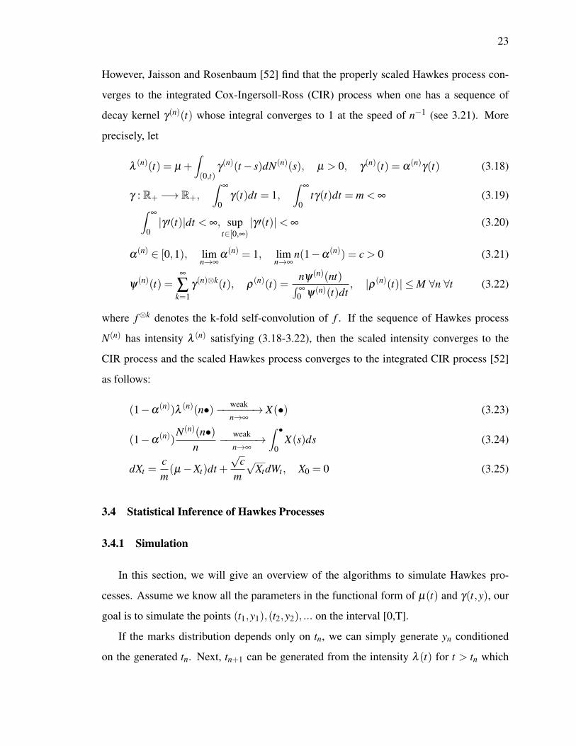
However, Jaisson and Rosenbaum [52] find that the properly scaled Hawkes process con-
verges to the integrated Cox-Ingersoll-Ross (CIR) process when one has a sequence of
decay kernel γ(n)(t) whose integral converges to 1 at the speed of n−1 (see 3.21). More
precisely, let
λ(n)(t) = µ +
∫(0,t)
γ(n)(t− s)dN(n)(s), µ > 0, γ
(n)(t) = α(n)
γ(t) (3.18)
γ : R+ −→ R+,∫
∞
0γ(t)dt = 1,
∫∞
0tγ(t)dt = m < ∞ (3.19)∫
∞
0|γ ′(t)|dt < ∞, sup
t∈[0,∞)
|γ ′(t)|< ∞ (3.20)
α(n) ∈ [0,1), lim
n→∞α(n) = 1, lim
n→∞n(1−α
(n)) = c > 0 (3.21)
ψ(n)(t) =
∞
∑k=1
γ(n)⊗k(t), ρ
(n)(t) =nψ(n)(nt)∫∞
0 ψ(n)(t)dt, |ρ(n)(t)| ≤M ∀n ∀t (3.22)
where f⊗k denotes the k-fold self-convolution of f . If the sequence of Hawkes process
N(n) has intensity λ (n) satisfying (3.18-3.22), then the scaled intensity converges to the
CIR process and the scaled Hawkes process converges to the integrated CIR process [52]
as follows:
(1−α(n))λ (n)(n•) weak−−−−−−→
n→∞X(•) (3.23)
(1−α(n))
N(n)(n•)n
weak−−−−−−→n→∞
∫ •0
X(s)ds (3.24)
dXt =cm(µ−Xt)dt +
√c
m√
XtdWt , X0 = 0 (3.25)
3.4 Statistical Inference of Hawkes Processes
3.4.1 Simulation
In this section, we will give an overview of the algorithms to simulate Hawkes pro-
cesses. Assume we know all the parameters in the functional form of µ(t) and γ(t,y), our
goal is to simulate the points (t1,y1),(t2,y2), ... on the interval [0,T].
If the marks distribution depends only on tn, we can simply generate yn conditioned
on the generated tn. Next, tn+1 can be generated from the intensity λ (t) for t > tn which

24
depends on (t1,y1), ...,(tn,yn). If the distribution of yn also depends on (tn−1,yn−1),
(tn−2,yn−2), ..., the algorithms can be modified accordingly.
Inverse CDF Transform
The first simulation algorithm for Hawkes processes appears in [56]. Suppose the in-
tensity is governed by the univariate Hawkes model in (3.9). Let ti be the arrival time and
τn = tn− tn−1 be the inter-arrival time. By (3.6), λ (t) = hn(t− tn−1) for t ∈ (tn−1, tn] where
hn(t) = gn(t)/(1−Gn(t−)) and g, G are the conditional pdf, cdf of τn given Ftn−1 . If Gn(t)
is continuous, hn(t) is simply the hazard function, and it can be shown that
Gn(τn) = 1− exp(−∫
τn
0hn(s)ds
)= 1− exp
(−∫ tn−1+τn
tn−1
λ (s)ds)
(3.26)
Given tn−1, we can generate tn = tn−1+τn by inverse cdf transform τn = G−1n (U), U ∼
Unif(0,1). However, the inversion needs to be done numerically, so this method is largely
superceded by Ogata’s modified thinning which we now discuss.
Ogata’s Modified Thinning
Ogata [57] introduces the modified thinning method which does not require numerical
inversion. The algorithm is based on the following theorem. Let N = (N1, ..,Nd) be a
multivariate point process with intensity (λ1, ..,λd) such that ∑di=1 λi(t) ≤ λ ∗(t) ∀t a.s.
(λ ∗(t) is an exogenously chosen deterministic rate function) and N∗ is the univariate non-
homogeneous Poisson process with intensity λ ∗(t). If each point tn in N∗ is given a mark yn
such that P(yn = i) = λi(tn)/λ ∗(tn), i = 1, ..,d, then (N∗1 , ..,N∗d ) has the same distribution
as (N1, ..,Nd).
The following algorithm generates a d-dimensional multivariate Hawkes process such
that λi(t) is decreasing between points and |λi(t)−λi(t−)| ≤ αi ∀t.
Ogata’s Modified Thinning [57]
1. n = 1, t0 = 0

25
2. Generate τn ∼ Exp(λ ∗n ) for some λ ∗n ≥ ∑di=1(λi(tn−1)+αi)
(Exp(λ ) is exponential distribution with rate λ )
3. Let tn = tn−1 + τn
4. Generate Un ∼ Unif(0,1)
5. if Un ∈ (∑k−1i=0 λi(tn)/λ ∗n ,∑
ki=0 λi(tn)/λ ∗n ] for some k ∈ 1, ..,d return tn and the point
is of type k (also generate yn|tn for MPP) , else discard tn (but keep the value for use
in next generation)
6. n = n+1, goto step 2
Simulation by Branching Structure
This method generates points using the branching structure representation of linear
marked Hawkes processes. Type j immigrants arrive according to a non-homogeneous
Poisson with rate µ j(t). Next the type- j parent arriving at tn produces type-i descendants
according to non-homogeneous Poisson with rate γi j(t − tn,yn) and the generation is re-
peated for each descendant until all of them exceed the pre-defined time T. Since all the
non-homogeneous Poisson processes are independent, the generations can be done in par-
allel, making this algorithm very suitable for parallel implementation.
Simulation by the Branching Structure [58]
1. Generate non-homogeneous Poisson processes with intensities µi(t), i = 1, ..,d on
[0,T ]
2. For each points tn, generate yn|tn3. Suppose tn is of type j, generates type-i descendants according to non-homogeneous
Poisson process with intensity γi j(t− tn,yn) on [tn,T ], i = 1, ..,d
4. repeat step 2, 3 for all descendants
The non-homogeneous Poisson process with intensity µ(t) on [0,T ] can be generated using
Lewis’ thinning algorithm [59]
1. generate N ∼ Poisson(µ∗) for some µ∗ ≥maxt∈(0,T ]µ(t)
2. generate Un ∼ Unif(0,1), n = 1, ..,N

26
3. Tn =U(n)T, n = 1, ..,N (U(n) is the order statistics of Un)
4. generate Vn ∼ Unif(0,1), i = 1, ..,N
5. return Tn if Vn ≤ (µ(Tn)/µ∗), n = 1, ..N; otherwise discard Tn
3.4.2 Estimation
Suppose we observe a point process from 0 to T and collect the event times and marks
(t1,y1), ..,(tN ,yN), now we would like to estimate the functions µ(t) and γ(t,y) in the
intensity λ (t) which drives the process N(t). We will summarize the various methods
appearing in the literature, but so far the focus is on unmarked process. In the special case
where the marks are independent and identically distributed (IID), the mark distribution
can be estimated separately from the point process.
If we assume µ(t) and γ(t) have some parametric representations, we can use Maxi-
mum Likelihood Estimation (MLE), Expectation Maximization (EM), or Generalized Me-
thod of Moments (GMM) to estimate the parameters. Otherwise, we need to rely on some
advanced non-parametric techniques to estimate the whole function curves.
Maximum Likelihood Estimation (MLE)
The log likelihood of a Hawkes process is given by [56]
log(L(θ)) =d
∑i=1
(−∫ T
0λi(t;θ)dt +
∫ T
0log(λi(t;θ))dNi(t)
)(3.27)
In the case of multivariate linear Hawkes process, it becomes
log(L(θ)) =−∫ T
0
(d
∑i=1
µi(t;θ)
)dt−
N
∑n=1
∫ T
tn
(d
∑i=1
γi,wn(t− tn;θ)
)dt
+N
∑n=1
log
(µwn(tn;θ)+ ∑
tm<tnγwn,wm(tn− tm;θ)
)(3.28)
The parameters in the Hawkes process can be estimated by maximizing the log-likeli-
hood. However, the numerical optimization is problematic as the log likelihood function is
usually quite flat (see [60, fig.2,3]) and may have a lot of local maxima (see [60, fig.4]).
27
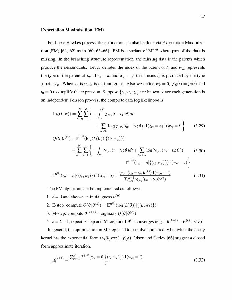
Expectation Maximization (EM)
For linear Hawkes process, the estimation can also be done via Expectation Maximiza-
tion (EM) [61, 62] as in [60, 63–66]. EM is a variant of MLE where part of the data is
missing. In the branching structure representation, the missing data is the parents which
produce the descendants. Let zn denotes the index of the parent of tn and wzn represents
the type of the parent of tn. If zn = m and wzn = j, that means tn is produced by the type
j point tm. When zn is 0, tn is an immigrant. Also we define w0 = 0, γi,0(t) = µi(t) and
t0 = 0 to simplify the expression. Suppose tn,wn,zn are known, since each generation is
an independent Poisson process, the complete data log likelihood is
log(L(θ)) =N
∑n=0
d
∑i=1
−∫ T
tnγi,wn(t− tn;θ)dt
+ ∑tm>tn
log(γi,wn(tm− tn;θ))1(zm = n)1(wm = i)
(3.29)
Q(θ |θ (k)) =Eθ (k)(log(L(θ))|(tk,wk))
=N
∑n=0
d
∑i=1
−∫ T
tnγi,wn(t− tn;θ)dt + ∑
tm>tnlog(γi,wn(tm− tn;θ))
Pθ (k)(zm = n|(tk,wk))1(wm = i)
(3.30)
Pθ (k)(zm = n|(tk,wk))1(wm = i) =
γi,wn(tm− tn;θ (k))1(wm = i)
∑m−1l=0 γi,wl(tm− tl;θ (k))
(3.31)
The EM algorithm can be implemented as follows:
1. k = 0 and choose an initial guess θ (0)
2. E-step: compute Q(θ |θ (k)) = Eθ (k)(log(L(θ))|(tk,wk))
3. M-step: compute θ (k+1) = argmaxθ Q(θ |θ (k))
4. k = k+1, repeat E-step and M-step until θ (k) converges (e.g. ‖θ (k+1)−θ (k)‖< ε)
In general, the optimization in M-step need to be solve numerically but when the decay
kernel has the exponential form αi jβi j exp(−βi jt), Olson and Carley [66] suggest a closed
form approximate iteration.
µ(k+1)i =
∑Nm=1Pθ (k)
(zm = 0|(tk,wk))1(wm = i)T
(3.32)

28
α(k+1)i j =
∑Nn=1 ∑
Nm=n+1Pθ (k)
(zm = n|(tk,wk))1(wm = i,wn = j)
∑Nn=11(wn = j)
(3.33)
β(k+1)i j =
∑Nn=1 ∑
Nm=n+1Pθ (k)
(zm = n|(tk,wk))1(wm = i,wn = j)
∑Nn=1 ∑
Nm=n+1(tm− tn)Pθ (k)
(zm = n|(tk,wk))1(wm = i,wn = j)(3.34)
Pθ (k)(zm = n|(tk,wk))1(wm = i,wn = j) =
α(k)i j β
(k)i j exp(−β
(k)i j (tm− tn))1(wm = i,wn = j)
µ(k)i +∑
m−1l=1 α
(k)i,wl
β(k)i,wl
exp(−β(k)i,wl
(tm− tl))(3.35)
Pθ (k)(zm = 0|(tk,wk))1(wm = i) =
µ(k)i 1(wm = i)
µ(k)i +∑
m−1l=1 α
(k)i,wl
β(k)i,wl
exp(−β(k)i,wl
(tm− tl))
(3.36)
In addition, the summation ∑m−1l=1 α
(k)i,wl
β(k)i,wl
exp(−β(k)i,wl
(tm− tl)) can be truncated after
exp(−β(k)i,wl
(tm− tl)) has decayed to a small value. The speed of EM is reported to be
10-100 times faster than MLE using Nelder-Mead and more importantly, MLE does not
converges within 500 iterations in practically all test cases while EM does [66].
Generalized Method of Moments (GMM)
Another method for statistical estimation beyond MLE is the Generalized Method of
Moments24 [67]. The idea is to find the parameters which minimize the difference between
theoretically moments in term of the unknown parameters and the empirical moments com-
puted directly from the data. If we have more moments than the number of parameters, the
method involves solving a weighted least squares problem.
Da Fonseca and Zaatour [68] obtain analytic moment expressions by restricting the
process to be univariate with exponential kernel and making use of the Markov property
in this special case. The authors claim that this method is extremely fast but no speed
comparison result is provided.
24Although GMM is consistent under some mild regularity conditions, unlike MLE, it is not asymptoticefficient among the class of consistent estimators.

29
Nonparametric Estimation
Without assuming any parametric form for µ(t) nor γ(t), some nonparametric methods
are developed recently to estimate the whole base rate and decay kernel functions. Similar
to parametric estimation, penalized MLE or GMM is used to find the function with desir-
able characteristics (e.g. smooth functions or sparse coefficients). Nonetheless, the non-
parametric method, which involves finding the unknown functions in infinite-dimensional
spaces, requires extensive computational effort and the underlying statistical construction
is usually much more involved than any parametric counterpart.
To the best of our knowledge, the first attempt in nonparameteric estimation of Hawkes
process is by Gusto and Schbath [69] in 2005. The authors express the kernel function of
the multivariate Hawkes process using B-splines [70] with equally spaced knots. The log
likelihood function involving the basis coefficients are then maximized numerically and the
optimal order for the B-splines basis as well as number of knots are determined using AIC
criteria [71].
Instead of B-splines, Reynaud-Bouret and Schbath [72] find the function within the
space of piecewise constant functions which minimizes the empirical L2-norm between the
true and estimated kernel functions. The method is later extended to multivariate cases [73]
with a Lasso type penalty [74] in the minimization objective.
On the other hand, the base and kernel functions can be estimated nonparametrically
in each M-step of EM as in [75], within the space C1(R+) with Good’s penalty ‖(√γ)′ ‖2
[76]. Using calculus of variations, the solution of each penalized maximization in M-step
can be found by solving the Euler-Lagrange equation numerically.
Instead of EM, Zhou et al. [77] use Minorize-Maximization (MM) algorithm [78], in
which EM is a special case. In the E-step of MM algorithm, Q(•|θ (k)) is any lower bound of
the objective function log(L(•)) such that Q(θ (k)|θ (k)) = log(L(θ (k))). It is then iteratively
maximized in the M-steps until convergence. In [77], the kernel functions are expressed
using a finite number of basis functions which are estimated nonparametrically in M-step
by solving the Euler-Lagrange equation.

30
Another approach is to use moment matching to find the kernel function as in [79–81].
In Bacry and Muzy [81], the authors derive the conditional moment density
E(dNi(t)|dN j(0)= 1,dy) of multivariate marked Hawkes process as the solution of Wiener-
Hopf equation [82] involving µi,γi j(t),gi j(y) for the case that the mark impact kernel is
piecewise constant. The conditional moment density can be estimated by any kernel den-
sity estimation technique and the Wiener-Hopf equation can be solved numerically via the
Nyström method [83].
3.4.3 Hypothesis Testing
Random Time Change
The classical method to test the goodness-of-fit of a point process model on R+ is
Ogata’s residual analysis [43]. Ogata calls tn =∫ tn
0 λ (s)ds the residual process25 and
according to the random time change theorem, the residual process should be close to
a standard Poisson process if the estimated intensity λ (t) is close to the true intensity
λ (t). The hypothesis that tn is a standard Poisson process can be tested by the following
methods:
1. QQ Plot [85] of τn = tn− tn−1 vs Exp(1).
2. Kolmogorov-Smirnov Test [86–88] to test τn ∼ Exp(1)
3. Ljung-Box Test [89] to test the lack of serial correlation of τn
Approximate Thinning
Another method to test goodness-of-fit is by thinning, which does not require inte-
gration of the intensity function. It is useful if the intensity function is estimated non-
parametrically. However, the thinned residual process is only approximately a Poisson
process.
25The terminology is not standard, Baddeley et al. [84] refer N(tn)−∫ tn
0 λ (s)ds as residual in order toextend the concept to higher dimension.

31
By Ogata’s modified thinning [57], we know that if there exists b > 0 such that b ≤
λ (t)∀t and we keep point tn with probability b/λ (tn), the thinned point process is a homo-
geneous Poisson process with rate b. However, the infimum b of the intensity function is
often close to 0, making the number of points in the thinned process very small and the test
to have little power. A remedy is to use approximate thinning [90] as follows: choose an
integer k N, select a point from t1, .., tN with probability of selecting tn proportional
to λ (tn)−1. Repeat the selection (without replacement) until k points are selected. The
resulting k points will be approximately a homogeneous Poisson process.
3.5 Applications of Hawkes processes
After the groundwork of basic theory and statistical inference for Hawkes processes,
we now unleash their power to model HF data. First, the readers are reminded about how
diverse the notion of stock trading frequency can be. According to the Trade And Quote
database (TAQ), between 9:30am to 4:00pm on May 2, 2014, there were 11 million quote
changes (limit + cancellation + market orders) and 0.3 million trades (market orders) for
SPDR S&P 500 ETF (SPY). In other words, on average there are 460 quote changes and
13 trades per second. If we take a snapshot every 5 minutes as in [32, 33], we will only
use 0.03% of trade data and 0.0007% of quote data. In comparison, Pathfinder Bancorp
(PBHC) only has 306 quote changes and 11 trades on the the same day, which means there
is a 35 minutes lag between trades on average and thus the 5 minutes snapshots will just
give a series of repeated information. Regardless of the sampling frequency, we are likely
to get some misleading result if we analyze the asynchronous data from a portfolio of liquid
and illiquid stocks using models with fixed intervals.
The construction of multivariate point processes shows that each variate can have a
completely different arrival intensity λi(t) from its peers’. Nonetheless, the multivariate
Hawkes process can still model the dependence structure easily via the γi j(t)’s, which are
estimated by duly considering all the asynchronous data of highest frequency without any
re-sampling.

32
Order arrivals and price changes are unarguably two of the most important elements
in high frequency trading. Using Hawkes processes, we can estimate their distributions
conditioned on all the historical HF asynchronous data, enabling us to give a more accurate
real time prediction of future event occurrences. In the following subsections, we are going
to highlight some of the literature which take advantage of Hawkes processes to model HF
data.
3.5.1 Modeling Order Arrivals
Bowsher [50]26 is the first to use Hawkes processes to model order arrivals. He uses
nonlinear Hawkes processes to allow for inhibitory effect and he considers two rate func-
tions Φi(x, t) = µi(t)+exp(x) and Φi(x, t) = max(µi(t)+x,εi), εi > 0, where both of them
guarantee that the stochastic intensity will be strictly positive at all times. For the deter-
ministic base rate µi(t), he exploits a piecewise linear function with knots at 9:30, 10:00,
11:00,...,16:00 while the decay kernel is the exponential function without marks. In addi-
tion, an extra term is included to represent the spillover effects from the previous trading
day.
Bowsher uses Maximum Likelihood Estimation (MLE) to estimate the parameters for
the bivariate point process of trade and quote of General Motor (GM), trading on NYSE
between 5 July 2000 to 29 August 2000. The model is found to be decent according to the
goodness-of-fit test using random time change.
Instead of modeling arrivals of all trades and quotes, Large [22] uses Hawkes processes
to model only the arrivals of aggressive orders, which are market orders depleting the queue
and limit orders falling inside the bid-ask spread, in order to study the resiliency of the
LOB. A LOB is called resilient if it reverts to its generic shape promptly after large trades.
The idea is that when a large trade causes the bid-ask spread to widen, the arrival intensity
of aggressive limit orders in a resilient LOB will surge so that the gap will be filled very
26Though Bowsher’s paper was published in 2007, the first draft appeared in 2002.

33
quickly. In order words, the cross-excitation effect γi j(t) from aggressive market orders to
aggressive limit orders should be reasonably large for a resilient LOB.
In addition to market orders and limit orders, Large also includes the cancellations of
limit orders as well as limit orders falling outside the best quotes. Therefore, he builds a
10-variate linear marked Hawkes process with exponential decay and mark impact kernel
to fit the HF data of Barclays (BARC), trading on LSE between 2 Jan 2002 to 31 Jan 2002.
The result shows that the widening of bid-ask spread indeed pumps up the intensities of
aggressive limit orders, causing the gap to be filled very quickly and hence making the
LOB resilient.
More examples of applications of Hawkes processes to order arrivals include the fol-
lowing papers: Muni Toke and Pomponio [91] use similar approach as Large [22] to model
trades-through, namely market orders which deplete the best queues and consume at least
one share in the second best. Muni Toke [92] designs a more realistic market simulator
using Hawkes processes with exponential kernel for order arrivals. Shek [93], Fauth and
Tudor [94] apply the Hawkes processes with volume mark on stock and FX market respec-
tively. Hewlett [95] models the arrival of market orders with Hawkes processes for single
period market making. Finally, Alfonsi and Blanc [96], Jaisson [97] tackle the problem of
optimal execution with market orders coming from multivariate Hawkes processes.
3.5.2 Modeling Price Jumps
Single Asset
Traditionally the events of price jumps are modeled by Poisson processes, which suffer
from the drawbacks mentioned in the introduction section. Again, Hawkes processes can
be applied to model price jumps, which often delineate clustering, self- and cross-excitation
behavior.
Bacry et al. [98] use Hawkes processes to model the price jumps, resulting in a model
which can reproduce the microstructure noise [99], Epps effect [100] and jump clustering,

34
while maintaining the coarse scale limit of Brownian diffusion. In their model, the trade
price X(t) has the dynamics
X(t) = N1(t)−N2(t) (3.37)
where N(t) = (N1(t),N2(t)) is a bivariate linear Hawkes process with exponential decay
kernel. N1(t),N2(t) represents the total number of upward and downward jumps respec-
tively. The authors make additional assumptions that the Hawkes process N has only cross-
excitation and coefficients are symmetric in order to simplify computation:
λ1(t) = µ +∫(0,t)
γ(t− s)dN2(t), λ2(t) = µ +∫(0,t)
γ(t− s)dN1(t) (3.38)
γ(t) = αe−β t (3.39)
According to the model, when X jumps up(down), λ2 (resp. λ1) increases, causing the
probability of jumping down (resp. up) to increase. Such cross-linkage generates the effect
of microstructure noise where the trade price is bouncing between best bid and best ask.
Due to the bid-ask bounce, it is well-known that the realized variance (annualized)
increases when the sampling frequency increases [101].
V (τ) =E
(1T
T/τ
∑n=0
(X((n+1)τ)−X(nτ))2
)(3.40)
=2µ
1−α/β
(1
(1+α/β )2 +
(1− 1
(1+α/β )2
)1− e−(α+β )τ
(α +β )τ
)(3.41)
Such an effect can be easily demonstrated by computing the expected realized variance
(3.41) of the jump model (3.37) and the result with µ = 0.16,α = 0.024,β = 0.11 is shown
in Fig.3.1. The authors apply the model to Euro-Bund futures and find a very good fit
between the observed and theoretical realized variance under this highly simplified model.
Let Y (t) = X(nt), then Y (t) is a coarse scale version of X(t). For example, if t in X is
in micro second and n = 60000, then t in Y will be in minute. When we look at the trade
price in a low frequency setting, Bacry et al. [23] show that the macroscopic Hawkes jump
model goes back to the classical model of Brownian motion due to the functional central
limit theorem for linear Hawkes process (3.13). Assuming that∫
∞
0 γ(t)dt < 1, then

35
0 50 100 150 200
0.3
0.35
0.4
Sampling Interval τ
Exp
ecte
dR
ealiz
edVo
latil
ityV
Figure 3.1. Volatility Signature Plot of Hawkes Jump Model
X(n•)√n
weak−−−−−−→n→∞
σW (•), σ2 =
2µ
(1−∫
∞
0 γ(t)dt)(1+∫
∞
0 γ(t)dt)2 (3.42)
It is interesting to see how the macroscopic variance σ2 is related to the microscopic
base rate µ and cross-excitation γ(t). As∫
∞
0 γ(t)dt approaches 1, the variance goes to ∞.
Jaisson and Rosenbaum [52] extend the model of Bacry et al. [98] for the case of nearly
unstable Hawkes process, where∫
∞
0 γ(t)dt ' 1, by constructing a sequence of kernel func-
tions whose integrals converge to 1 at the speed of n−1. They show that the properly scaled
price process converges to Brownian diffusion with Heston stochastic volatility [102]. The
full result is stated below.
X (n)(t) = N(n)1 (t)−N(n)
2 (t) (3.43)
λ(n)1 (t) = µ +
∫ t
0γ(n)1 (t− s)dN(n)
1 (s)+∫ t
0γ(n)2 (t− s)dN(n)
2 (s) (3.44)
λ(n)2 (t) = µ +
∫ t
0γ(n)2 (t− s)dN(n)
1 (s)+∫ t
0γ(n)1 (t− s)dN(n)
2 (s) (3.45)(∫∞
0γ(n)1 (t)dt +
∫∞
0γ(n)2 (t)dt
)< 1, γ
(n)i (t) = α
(n)γi(t) (3.46)
γi : R+ −→ R+,∫
∞
0(γ1(t)+ γ2(t))dt = 1 (3.47)

36
∫∞
0t(γ1(t)+ γ2(t))dt = m < ∞,
∫∞
0|γi′(t)|dt < ∞, sup
t∈[0,∞)
|γi′(t)|< ∞ (3.48)
α(n) ∈ [0,1), lim
n→∞α(n) = 1, lim
n→∞n(1−α
(n)) = c > 0 (3.49)
ψ(n)(t) =
∞
∑k=1
(γ(n)1 + γ
(n)2
)⊗k(t), ρ
(n)(t) =nψ(n)(nt)∫∞
0 ψ(n)(t)dt, |ρ(n)(t)| ≤M ∀n ∀t
(3.50)
Under the conditions of (3.43 - 3.50),
X (n)(n•)n
weak−−−−−−→n→∞
Y (•) (3.51)
dYt =
√Vt
1−∫
∞
0 |γ1(t)− γ2(t)|dtdW 1
t , Y0 = 0 (3.52)
dVt =cm
(2µ
c−Vt
)dt +
√Vt
mdW 2
t , V0 = 0 (3.53)
Conditions (3.43 - 3.45) is just a bivariate Hawkes model (with both self- and cross-
excitation) but now we have a different γ(n)i (t) for each n that use to scale the time. The rest
are the regularity conditions similar to the univariate nearly unstable Hawkes process (3.25)
and the most important one is (3.49) which states that α(n) converges to one at the speed
of n−1. However, the interesting result is that instead of converging to an integrated CIR,
the price dynamics formed by the difference between two Hawkes processes converges to
a stochastic volatility model.
Two Assets
To model the Epps effect, Bacry et al. [98] consider the two-asset case with prices
(X1(t),X2(t)) given by
X1(t) = N1(t)−N2(t), X2(t) = N3(t)−N4(t) (3.54)
λi(t) = µi +4
∑j=1
∫(0,t)
αi j exp(−β (t− s))dN j(s), i = 1, ..,4 (3.55)

37
(N1(t), ..,N4(t)) is a 4-variate Hawkes process with exponential kernel where βi j = β . The
coupling of excitation effects is constrained to have the form
α =
0 α12 α13 0α12 0 0 α13α31 0 0 α340 α31 α34 0
(3.56)
In this case, there is a closed form representation for the realized correlation, which van-
ishes when the sampling interval goes to zero (Epps effect).
If we assume µ1 = µ2, µ3 = µ4, α12 = α34 = 0, (∫
∞
0 γ13(t)dt)(∫
∞
0 γ31(t)dt) < 1, then
the macroscopic bivariate asset prices converges to correlated Brownian diffusion [23]
1√n
(X1(n•)X2(n•)
)weak−−−−−−→n→∞
√2(√
ν1W1(•)+√
ν2∫
∞
0 α13(t)dtW2(•)√ν1∫
∞
0 α31(t)dtW1(•)+√
ν2W2(•)
)(1− (
∫∞
0 γ13(t)dt)(∫
∞
0 γ31(t)dt))3/2 (3.57)
ν1 = µ1 +
(∫∞
0γ13(t)dt
)µ3, ν2 = µ3 +
(∫∞
0γ31(t)dt
)µ1 (3.58)
(W1(•),W2(•)) is standard 2-dimensional Brownian motion
This convergence result gives us an explicit formula to estimate the macroscopic correlation
from the asynchronous high frequency data.
As a final remark, under this jump representation, the observed trade price is not some
hidden continuous fair value plus some microstructure noise as in [103]. It is the result of
the trading actions between buyers (N1,N3) and sellers (N2,N4) on a fixed price grid. There
is no such thing as high frequency volatility or correlation since prices are not diffusions
but pure-jump processes in the HF scale. Volatility and correlation are only meaningful
when we look at the coarse scale diffusion approximation at low frequency, but those low
frequency representation parameters can be computed directly from the high frequency
jump model characteristics.

38
3.5.3 Modeling Jump-Diffusion
Duffie et al. [104, 105] propose the affine jump-diffusion X(t), which has the following
structure.27
dX(t) = (k0(t)+ k1(t)X(t))dt +(h0(t)+h1(t)X(t))dW (t)+ζ dN(t) (3.59)
λ (t) = a0(t)+a1(t)X(t) (3.60)
The jump intensity λ (t) of N(t) is an affine function of X(t), which depends on the
Brownian motion W (t) and the jump process N(t), with jump size ζ drawn from a fixed
distribution. When k0 = βθ ,k1 =−β ,h0 = h1 = 0,a0 = 0,a1 = 1,ζ = α , we can see that
λ (t) = X(t) and dλ (t) = β (θ −λ (t))dt +αdN(t). Hence in this case N(t) is the Hawkes
process with exponential kernel.
Zhu [106] derives some convergence results when ζ is a constant and the diffusion part
is a CIR process.
dX(t) = β (µ−X(t))dt +σ√
X(t)dW (t)+αdN(t) (3.61)
λ (t) = a0 +a1X(t) (3.62)
Aït-Sahalia et al. [107] model the contagion of financial crisis with the Hawkes jump-
diffusion where the price dynamic Xi(t) is given by
dXi(t) = µidt +√
Vi(t)dW Xi (t)+Zi(t)dNi(t) (3.63)
dVi(t) = κi(θi−Vi(t))dt +ηi√
Vi(t)dWVi (t) (3.64)
The diffusion part is the Heston stochastic volatility model and the jump part is a multi-
variate Hawkes process modeling the clustering and propagation of jumps among multiple
assets. Zi(t) corresponds to the jump size and direction.
3.5.4 Measuring Endogeneity (Reflexivity)
In term of the Hawkes branching structure representation of events arrivals, Filimonov
et al. [108, 109] portray immigrants as exogenous news whereas the descendants are en-27We show the one dimensional case for simplicity.

39
dogenous incidents. In the context of price movements in the stock or commodity market,
immigrants are the price discovery due to orders from informed traders, who react to ex-
ternal information, whereas the descendants are the destabilizing ripples created by noise
traders, who engage in herding [110], momentum trading [111] and parasite trading [112]
etc.
Under the univariate linear Hawkes model with exponential decay kernel and constant
base rate, the expected number of direct descendants per individual (branching coefficient)
is given by
n =∫
∞
0γ(s)ds =
∫∞
0αe−β sds = α/β (3.65)
For a given immigrant, the expected number of descendants in all generations is n+ n2 +
n3 + ...= n/(1−n) if n < 1, so the ratio of descendants (non-immigrants) vs total popula-
tion is
descendantsdescendants + immigrant
=n/(1−n)
n/(1−n)+1= n (3.66)
Therefore, the branching coefficient n characterizes the degree of endogenous feedback
activities while the base rate µ measures the arrival rate of exogenous information.
Using E-mini S&P futures as proxy, Filimonov and Sornette [108] find that the level of
endogeneity (reflexivity28) n in the US market has gone from 0.3 in 1998 to 0.7 in 2007.
Moreover, for the flash crash of May 6, 2010, n reached a peak of 0.95.
Nonetheless, using the power law decay kernel, Hardiman et al. [114] challenge the
result of Filimonov and Sornette [108] by reporting that the branching ratio n has always
been close to one since 1998 and that the market could be a critical Hawkes process [51],
but Filimonov and Sornette [115] refute that the power law kernel is sensitive to outliers
in addition to other counter arguments. Later Hardiman and Bouchaud [116] devised a
nonparametric estimation of the branching ratio in term of moments, but the result depends
heavily on the window size used in the empirical moment computation.
28Filimonov and Sornette [108] borrow this term from Soros [113].

40
3.6 A Brief History of Hawkes processes
Hawkes processes are proposed by Hawkes [42] in 1971 in order to model contagious
processes like epidemics, neuron firing and particle emission, where the occurrences of
events trigger further events. Although the intensity of Cox processes [117], introduced
in 1955, are stochastic, they are determined before the events are unfolded29. In order to
portray the excitation behavior in contagious processes, Hawkes extends the model in such
a way that the intensity is a predictable stochastic process with an intuitive autoregressive
form, which allows it to adapt to events that happen over time.
After Hawkes’ seminal paper, a number of theoretical developments include the branch-
ing structure representation by Hawkes and Oakes [46] in 1974, the Markov property for
the intensity with exponential decay kernel by Oakes [45] in 1975, the MLE for Hawkes
processes by Ozaki [56] in 1979, Ogata’s modified thinining simulation algorithm [57] in
1981, nonlinear Hawkes processes by Brémaud and Massoulié [48] in 1996, Nonparamet-
ric Estimation by Gusto and Schbath [69] in 2005, EM for Hawkes processes by Veen and
Schoenberg [60] in 2008 and the functional central limit theorem for Hawkes processes by
Bacry et al. [23], Jaisson and Rosenbaum [52], Zhu [53] in 2013.
Although the first application of Hawkes processes to earthquake occurrences appeared
in 1982 [44], it was not until 1988 [43] that Hawkes processes received much attention.
Since then, the versatility of Hawkes model was leveraged in seismology [43, 118], finance
(risk and credit default modeling) [119, 120], social networks [121, 122], neuroscience
[123, 124] etc. (see [125, 126] for more applications).
The use of Hawkes processes in HF financial data modeling starts with Bowsher [50]
in 200730 and then Large [22] in the same year. Both authors exploit Hawkes processes
so as to describe the interactions between order arrivals of different types. Later, Aït-
Sahalia et al. [107] and Bacry et al. [98] employ Hawkes processes to reproduce clustering
in jump diffusion and pure-jump process representation of stock prices in 2010 and 2013
respectively. On the other hand, an interesting idea appears in Filimonov and Sornette
29For processes on R+, it means their intensity is F0 measurable.30Though Bowsher’s paper was published in 2007, the first draft appeared in 2002.

41
[108] in 2012 which utilizes the branching coefficient of linear Hawkes model to measure
the level of endogenous activities in the US stock market, though the debate about the
validity of the result is still going on [114–116].

42

43
4. JOINT MODELING OF PRICES AND ORDER ARRIVALS
4.1 Introduction
The joint modeling of prices and order arrivals has not yet received much attention
in the mathematical finance literature. All the existing market-making models assume that
prices are independent from order arrivals, which is clearly far from the truth. For example,
when a large buy market order depletes the best ask queue, the ask price can only move
up. However, when you model the price and order arrival as two independent processes,
roughly half of the time price will go down with the arrival of buy order. Such an unrealistic
scenario produces a large phantom profit for the market maker and cause the average profit
of the market-making model to be overstated.
Besides, price is commonly modeled as diffusion whereas in high-frequency setting
price is a pure-jump process living on a fixed price grid. Moreover, each jump has two
components, namely time and magnitude. Diffusion can only describe the magnitude but
cannot model the timing of the jump and its dependency on the order arrival history. The
simplest way is to replace the diffusion with a Poisson process. However, it has been
documented that order flow has clustering and long memory properties [18, 19] and so a
self-exciting point process may be a better alternative.
Bacry and Muzy [127] model the mid-price and market buy and sell order as a 4-variate
Hawkes processes (T+,T−,N+,N+) where T±,N± denotes the buy/sell market order and
upward/downward jump of mid-price respectively. Although the price jump and market
order are now correlated via the cross-excitation, the problem of price goes down with a
buy market order still remains. In addition, multivariate Hawkes processes is by definition
a simple point process, meaning that price and market order cannot jump at the same time,
but this assumption contradicts the fact that price and market order always jump together
upon the arrival of aggressive market order that depletes the whole best bid/ask queue.

44
The authors work around the issue with some tricks that introducing a small delay ∆t to
the price jump and describe the excitation effect from market order to price jump as Dirac
delta function as ∆t goes to 0.
In this chapter, we make use of a simple technique developed in 60’s [128] for Pois-
son random variables to model the dependency structure of jump processes. Namely if
N1 = N′1 +U ′, N2 = N′2 +U ′, where (N′1,N′2,U
′) are independent Poisson random vari-
ables, then (N1,N2) have the so-called bivariate Poisson distribution. Co-jumps as well
as the dependency of (N1,N2) are modeled by the common component U ′. In our model,
(N′1,N′2,U
′) are not some latent processes but in fact some directly observable order book
events which we are going to describe shortly.
As a remark, our model does not aim to describe the full dynamics of a limit order
book, instead we strive to depict the relationship of the best bid/ask price with the order
arrivals using a tractable point process model. In many trading applications, traders will
only consider limit orders in the best bid/ask as the chance of execution beyond the best
quotes is simply too low (e.g. less than 3% for E-mini S&P future [21]). The utmost
concern of the traders is when the market orders arrive to fill their limit orders, so the
activities outside the best quotes have little value to them. Moreover, the practice of quote
stuffing1 [129] and spoofing2 [130] render the information content of the limit order book
questionable, especially beyond the best quotes. As a result, the benefit of a full order book
model may not justify the added nontrivial complexity and this may explain the emergence
of reduced-form models which focus only on the top of the book [131, 132].
4.2 Joint Modeling of Prices and Order Arrivals
We classify all orders which affect the top of book into twelve categories according
to type (limit, market, cancellation), direction (buy, sell) and aggressiveness similar to
[18, 22]. We follow the definition of [22] that aggressive orders are the ones which move the
bid or ask price. To be more precise, aggressive market order is the one which completely
1Rapid placement and cancellation of large amount of limit orders.2submission of limit orders to create an illusion of demand/supply imbalance
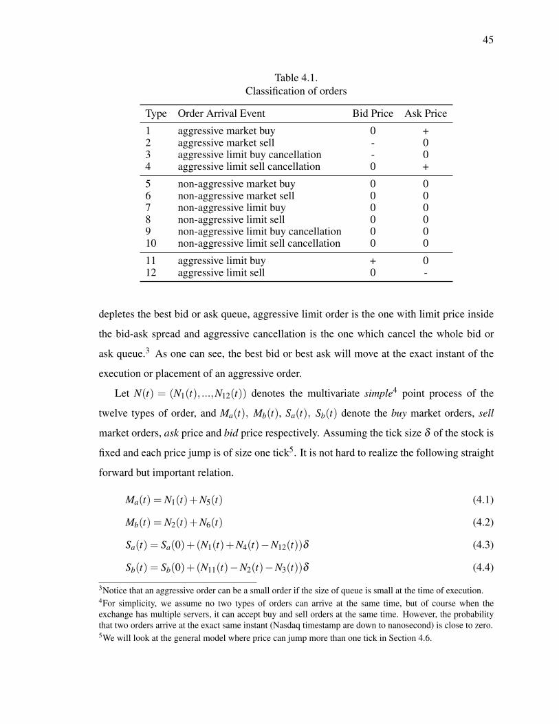
45
Table 4.1.Classification of orders
Type Order Arrival Event Bid Price Ask Price
1 aggressive market buy 0 +2 aggressive market sell - 03 aggressive limit buy cancellation - 04 aggressive limit sell cancellation 0 +
5 non-aggressive market buy 0 06 non-aggressive market sell 0 07 non-aggressive limit buy 0 08 non-aggressive limit sell 0 09 non-aggressive limit buy cancellation 0 010 non-aggressive limit sell cancellation 0 0
11 aggressive limit buy + 012 aggressive limit sell 0 -
depletes the best bid or ask queue, aggressive limit order is the one with limit price inside
the bid-ask spread and aggressive cancellation is the one which cancel the whole bid or
ask queue.3 As one can see, the best bid or best ask will move at the exact instant of the
execution or placement of an aggressive order.
Let N(t) = (N1(t), ...,N12(t)) denotes the multivariate simple4 point process of the
twelve types of order, and Ma(t), Mb(t), Sa(t), Sb(t) denote the buy market orders, sell
market orders, ask price and bid price respectively. Assuming the tick size δ of the stock is
fixed and each price jump is of size one tick5. It is not hard to realize the following straight
forward but important relation.
Ma(t) = N1(t)+N5(t) (4.1)
Mb(t) = N2(t)+N6(t) (4.2)
Sa(t) = Sa(0)+(N1(t)+N4(t)−N12(t))δ (4.3)
Sb(t) = Sb(0)+(N11(t)−N2(t)−N3(t))δ (4.4)
3Notice that an aggressive order can be a small order if the size of queue is small at the time of execution.4For simplicity, we assume no two types of orders can arrive at the same time, but of course when theexchange has multiple servers, it can accept buy and sell orders at the same time. However, the probabilitythat two orders arrive at the exact same instant (Nasdaq timestamp are down to nanosecond) is close to zero.5We will look at the general model where price can jump more than one tick in Section 4.6.

46
Through those remarkably simple equations (4.1)-(4.4), we can observe the dependency
of price and order arrivals via the common components N1 and N2. For instance, when there
is aggressive buy market order (type 1), both the buy market order point process Ma(t) and
ask price Sa(t) will jump at the same time (co-jump), but they can also jump separately
upon the arrival of other order types. From the equations, we can also recognize ask price
cannot go down with a buy market order (type 1 or 5).
This is in sharp contrast with the approach in [127] where the prices and market orders
are modeled as a simple multivariate point process. The first issue is that the prices always
jump at the instant of aggressive orders, but under the simple point process assumption in
[127], price jump and order arrival happen at the same time with probability zero. Second,
even if the ask price can be described as positively correlated with the buy market order,
there is still a non-zero probability that ask price goes down after a buy market order.
The bid-ask spread ∆(t) = Sa(t)−Sb(t) in our model is given by
∆(t) = (Sa(0)−Sb(0))+(N1(t)+N2(t)+N3(t)+N4(t)−N11(t)−N12(t))δ (4.5)
If we do not put any constrain on the point processes (N1(t), ..,N12(t)), there is no guarantee
that ∆(t) will be always greater than or equal to δ . Nonetheless if we look carefully at type
11 and type 12 orders (limit orders inside the spread), they can only appear when ∆(t−)> δ
and as a result ∆(t) will not shrink below δ . To put this constrain in the model, the simplest
way to restrict the intensity of the point process, using the fact that when the intensity is 0
at time t, the probability that an event happens at time t is zero [36, T12, p.31]. Let λi(t)
denote the stochastic intensity of the point process Ni(t), we thus impose the condition6
that
λ11(t) = µ11(t)1(∆(t−)> δ ) (4.6)
λ12(t) = µ12(t)1(∆(t−)> δ ) (4.7)
where µ11(t) and µ12(t) is any predictable non-negative stochastic processes.
6We can also use the equivalent form λi(t) = µi(t)1(∆(t)> δ ), see [36, T10, p.29] for proof.

47
4.3 One-Tick Bid-Ask Spread Model
For highly liquid stocks, the bid-ask spread ∆(t) can be one tick 99% of the time [133].
This kind of order book resiliency can be easily reproduced by a large µ11(t) or µ12(t). N11
and N12 will be activated right after the bid-ask spread is widen by the shock N1,N2,N3 or
N4. Provided that µ11(t) or µ12(t) is large enough, the aggressive limit order will arrive
quickly to fill the gap in the bid-ask spread. In fact, µ11(t)+µ12(t) may be used as a first
order measure7 of the resiliency of the order book.
In this case, bid and ask prices will always move in lockstep, so we only need to model
the mid-price S(t), which is given by (4.9)
S(t) =(Sa(t)+Sb(t))/2 (4.8)
=S(0)+(N1(t)−N2(t)−N3(t)+N4(t)+N11(t)−N12(t))δ/2 (4.9)
If we assume that N11 ' N12, the model enjoys a further simplification (4.10) as N11,N12
cancel each other. We would like to stress that since N11,N12 can only jump when the bid-
ask spread is larger than one tick, the overall impact on the price dynamics for liquid stocks
is limited even if the approximation N11 ' N12 is crude.
S(t) = S(0)+(N1(t)−N2(t)−N3(t)+N4(t))δ/2 (4.10)
4.4 Multivariate Hawkes Process
The simplest way to complete the specification of the model is to assume N1, ..,N12
are independent Poisson processes; nonetheless the assumption of independent arrival is
often rejected in the literature. In the classical study, Biais et al. [18] document the so-
called diagonal effect, which means the next order is more likely to have same type as
the previous one, and similar findings are also reported in [19, 134, 135]. In particular,
Tóth et al. [19] show that the dominant reason for such kind of persistent order flow is due
to order splitting, rather than herding. Since large institutions often split large orders into
7A better measure of resiliency is the time for the queue to return back to its normal size after a shock, butµ11(t),µ12(t) will be irrelevant after the first order is placed inside the spread.

48
small pieces and then continuously trade for hours or even days, the observed long memory
characteristics makes perfect sense.
Because of the above reasons, we will use a point process with stochastic intensity to
represent our order arrivals. As described in Chapter 3, multivariate Hawkes process [42]
is a popular self-exciting point process with intensity λi(t) depends on its own history in
the following form.
λi(t) = µi(t)+ ∑j≥1
∫(−∞,t)
γi j(t− s)dN j(s) = µi(t)+ ∑tn<t
γi,wn(t− tn) (4.11)
where wn is the type of the point tn and µi(t),γi j(t) are some non-negative functions. Using
the Hawkes model, the diagonal effect can be generated by large γii(t), which increases the
intensity of type i order upon its own arrivals.
For type 11,12 orders, their intensities are constrained to be 0 when ∆(t−) = δ . One
possibility is to multiply (4.11) with the indicator function 1(∆(t−) > δ ), resulting in the
so-called constrained Hawkes process [136]. The constrained Hawkes process will consist
of a latent unconstrained Hawkes process and the observed process will be the thinned
unconstrained Hawkes process with probability 1(∆(t−) > δ ). However, we opt to avoid
this complicated structure and we will assume the intensities of type 11,12 are of the form.
λ11(t) = µ111(∆(t−)> δ ) (4.12)
λ12(t) = µ121(∆(t−)> δ ) (4.13)
where µ11,µ12 are non-negative constants. N(t) = (N1(t), ...,N10(t)) will be modeled as a
10-variate (unconstrained) Hawkes process.
The reason for not using constrained Hawkes process is that since only the first limit
order placed inside the spread are aggressive and the bid-ask spread is one tick most of
the time for liquid stocks, the total number of type 11,12 orders is tiny and hence their
excitation effects on other order types are insignificant. On the other hand, the intensities
of aggressive limit order N11,N12 are induced by the presence of gap in the bid-ask spread
rather than the arrivals of other orders shortly before; therefore the cross-excitation effects
on N11,N12 from other orders will be negligible compared with the parameters µ11 or µ12
(see [22]).

49
Without the cross-linkage of the constrained components, the estimation will be much
easier. The multivariate Hawkes process (without 11,12) can be estimated using Maximum
Likelihood Estimation (MLE) or Expectation Maximization (EM) and µ11 and µ12 can be
simply estimated by the inverse of average arrival times of the type 11,12 orders during the
active period.
In the sequel, we will focus on the Markovian exponential kernel with a constant base
rate.
γi j(t) = αi j exp(−βit) (αi j ≥ 0, βi > 0) (4.14)
µi(t) = µi (4.15)
The reason is that under this condition, the intensity λ (t) = (λ1(t), ..,λ10(t)) is a Mark-
ov process [20, 45] (see also 5.2.2) and can be expressed in the form of SDEs (4.16). Hence,
(λ (t),N(t)) is also a Markov process even though N(t) depends on its whole history.
dλi(t) = βi(µi−λi(t))dt +d
∑j=1
αi jdN j(t) (4.16)
4.5 Scaling Limit
Assuming the one-tick spread model with N11 ' N12 (4.10), the change in mid-price
equals
∆S(t) = S(t)−S(0) = (N1(t)−N2(t)−N3(t)+N4(t))δ/2 = a>N(t) (4.17)
where a = (δ/2)[1, −1, −1, 1, 0, 0, 0, 0, 0, 0]> and N(t) = [N1(t), ...,N10(t)]>. The
following theorem shows that under certain regularity conditions, the pure-jump mid-price
converges weakly to a Brownian motion.
Theorem 4.5.1 (Scaling Limit of Mid-price)
Let Γ = [∫
∞
0 γi j(t)dt]i, j and Σ = diag((I10−Γ)−1µ). If the spectral radius of Γ < 1 and∫∞
0√
tγi j(t)dt < ∞ ∀i, j, then
√n(
∆S(•n)/n−•a>(I10−Γ)−1µ
)weak−−−−−−→n→∞
a>(I10−Γ)−1Σ
1/2W (•) (4.18)

50
Proof Since the spectral radius of Γ < 1 and∫
∞
0√
tγi j(t)dt < ∞, by the functional central
limit theorem for Hawkes process [23, Corollary 1], we have
√n(
N(•n)/n−•(I10−Γ)−1µ
)weak−−−−−−→n→∞
(I10−Γ)−1Σ
1/2W (•) (4.19)
Notice that ∆S(t) = a>N(t) and f (N) = a>N is continuous (a is a constant vector). Hence
result follows from the continuous mapping theorem.
In other words,
∆S(nt)' (a>(I10−Γ)−1µ)(nt)+(a>(I10−Γ)−1
Σ1/2)(√
nW (t)) (4.20)
On a macroscopic scale, ∆S(nt) behaves like a diffusion with variance (a>(I10 − Γ)−1
Σ(I10−Γ>)−1a)(nt). Therefore under a coarser time scale, our pure-jump model agrees
with the diffusion model commonly used to characterize longer term price movement.
4.6 General Model with Volume and Jump Size
Though less common, the price jumps caused by the aggressive orders can be larger
than one tick. Therefore in addition to the random jump times τn ∈R+, we add the random
marks ξn ∈N which correspond to the jump sizes (in ticks) of the aggressive orders (ξn = 0
for non-aggressive orders). Moreover, we add another mark vn corresponds to the volumes
of the orders.
The multivariate marked Hawkes process now becomes Ni(dt×dv×dξ ) and the com-
pensator will be of the form λi(t)µi(t,dv×dξ )dt where λi(t) is the intensity of the ground
process Ni(dt ×R+×N) and µi(t,dv× dξ ) is the conditional mark (jump and volume)
distribution. To simplify the presentation, we will use the notation Ni(dt× dv) = Ni(dt×
dv×N) and (Ni +N j)(dt × dv× dζ ) = Ni(dt × dv× dζ )+N j(dt × dv× dζ ). The joint
model of prices and market orders now becomes:
Ma(dt×dv) = (N1 +N5)(dt×dv) (4.21)
Mb(dt×dv) = (N2 +N6)(dt×dv) (4.22)

51
Sa(t) = Sa(0)+δ
∫(0,t]×R+×N
ξ (N1 +N4−N12)(dr×dv×dξ ) (4.23)
Sb(t) = Sb(0)+δ
∫(0,t]×R+×N
ξ (N11−N2−N3)(dr×dv×dξ ) (4.24)
For the one-tick spread model with N11 ' N12, it becomes
Ma(dt×dv) = (N1 +N5)(dt×dv) (4.25)
Mb(dt×dv) = (N2 +N6)(dt×dv) (4.26)
S(t) = S(0)+(δ/2)∫(0,t]×R+×N
ξ (N1−N2−N3 +N4)(dr×dv×dξ ) (4.27)
4.7 Numerical Illustration
In this section, we provide some numerical results in fitting the Hawkes model to the
tick data from Nasdaq TotalView-ITCH. TotalView is a message level database where all
the order additions, cancellations and executions8 are recorded in an amazing nano-second
precision and this allows us to observe the extreme short burst of arrivals not possible in
database time-stamped in seconds. However, we would like to point out there is a major
issue in our analysis with only Nasdaq data. Nasdaq exchange only matches about 20% of
the total volume in the US equity market, so the classification of orders using only Nasdaq
data will potentially overstate the number of aggressive orders and understate the number
of non-aggressive orders. We remind our readers the result in this section is more of an
illustration in fitting the Hawkes model rather than an empirical study of US equity market.
4.7.1 Summary Statistics
The background activities of the stock market is well-known to be higher around open
(9:30am) and close (4:00pm) than that during the mid-day [22, 50]. One way is to fit
a spline [70] to the base rate µ(t); however we would like to make our lives easier by
focusing on the period 12:00 - 2:00pm and assuming the µ(t) is constant over this period.
8Nasdaq splits a market order into pieces (with same time-stamp) when it is executed against several limitorders but we combine them as one single market order during our processing. Also, market orders executedagainst hidden limit orders are ignored in this study.

52
Table 4.2.Summary statistics of QQQ on June 2, 2014 (12pm-2pm)
Type Description Count % Count Avg Rate (/s) Avg Size
1 aggressive market buy 190 0.08% 0.0264 1,0402 aggressive market sell 171 0.08% 0.0238 6673 aggressive limit buy cancellation 164 0.07% 0.0228 6854 aggressive limit sell cancellation 106 0.05% 0.0147 5445 non-aggressive market buy 312 0.14% 0.0433 6706 non-aggressive market sell 210 0.09% 0.0292 8747 non-aggressive limit buy 54,187 24.19% 7.5260 1,0068 non-aggressive limit sell 53,332 23.80% 7.4072 1,0619 non-aggressive limit buy cancellation 58,481 26.10% 8.1224 897
10 non-aggressive limit sell cancellation 56,265 25.11% 7.8146 92711 aggressive limit buy 316 0.14% 0.0439 84212 aggressive limit sell 315 0.14% 0.0438 681
Figure 4.2 shows the summary statistics of Powershares QQQ Trust (Nasdaq 100 in-
dex ETF) (QQQ). It is well-known that the activities of limit order revisions dominate the
market and it is reflected clearly in the table that 99.2% of the orders are type 7-10.
02
00
40
06
00
time
no.
of
ord
ers
pe
r se
co
nd
12:00 12:30 13:00 13:30 14:00
Figure 4.1. Activities ofQQQ (all order types) onJune 2, 2014
02
46
8
time
no.
of
ord
ers
pe
r se
co
nd
12:00 12:30 13:00 13:30 14:00
Figure 4.2. Activities ofQQQ (type 1-6) on June 2,2014
Figure 4.1 shows the total no. of orders (all types) per second of QQQ during 12-2pm,
June 2, 2014, but the chart is not very useful as it is masked by the activities of limit order
revisions. Figure 4.2 shows that QQQ has less than 10 type 1-6 orders per second albeit
QQQ is one of the most liquid stocks in US.

53
4.7.2 Volume Distribution
1
Den
sity
0 2 4
0.0
0.2
0.4
0.6
2
Den
sity
0 2 4
0.0
0.1
0.2
0.3
0.4
0.5
3
Den
sity
0 1 2 3 4
0.0
0.2
0.4
0.6
0.8
4
Den
sity
0 1 2 3 4
0.0
0.2
0.4
0.6
0.8
5
Den
sity
0 2 4
0.0
0.2
0.4
6
Density
0 2 4
0.0
0.1
0.2
0.3
0.4
0.5
7
Density
0 2 4
0.0
0.2
0.4
0.6
0.8
8
Density
0 2 4
0.0
0.2
0.4
0.6
0.8
9
Density
0 2 40.0
0.2
0.4
0.6
0.8
10
Density
0 2 4
0.0
0.2
0.4
0.6
0.8
Figure 4.3. Histogram of log10(volume)
Before we study the arrivals timing of the orders, let’s look at the histograms of the
log10(volume) in Figure 4.3. The volume distributions of all order types are similar, with
log10(volume) roughly normal with mean 2.5 (300 shares) and standard deviation 0.7.
However, there is a higher-than-expected concentration of small orders in type 1,2,5,6,9,10.
We believe they are the so-called pinging orders [137] that HFT firms use to detect hidden
orders. If we remove those tiny orders, the mean and standard deviation of the log10(vol-
ume) change to around 2.7 (500 shares) and 0.5 and the histogram and QQ plots without
tiny orders are shown in Figure 4.4-4.5.

54
1
De
nsity
1 2 3 4 5
0.0
0.1
0.2
0.3
0.4
0.5
0.6
2
De
nsity
1 2 3 4 50.0
0.1
0.2
0.3
0.4
0.5
0.6
3
De
nsity
1.0 2.5 4.0
0.0
0.2
0.4
0.6
0.8
4
De
nsity
1.0 2.5 4.0
0.0
0.2
0.4
0.6
0.8
5
De
nsity
1 2 3 4 5
0.0
0.1
0.2
0.3
0.4
0.5
0.6
6
Density
1 2 3 4 5
0.0
0.1
0.2
0.3
0.4
0.5
7
Density
1 2 3 4 5
0.0
0.2
0.4
0.6
0.8
8
Density
1 2 3 4 5
0.0
0.2
0.4
0.6
0.8
9
Density
1 2 3 4 50.0
0.2
0.4
0.6
0.8
10
Density
1 2 3 4 5
0.0
0.2
0.4
0.6
0.8
Figure 4.4. Histogram of log10(volume) (without tiny orders)
Figure 4.5. QQ plots of log10(volume) vs normal distribution (without tiny orders)

55
4.7.3 Timing Distribution
In this section, we will look at the distribution of order arrival times. However, before
we look at the real data, we would like to try out the classical QQ plots on simulated scenar-
ios. In Figure 4.6 and 4.7, we show the inter-arrivals time of a simulated Hawkes process
(µ = 0.01,αi j = 100,β j = 1000,N = 60,000) as well as the fitted residuals. Visually there
is not much difference, but from the p-value of the Kolmogorov–Smirnov goodness-of-fit
test in Table 4.8, you can see the inter-arrival times fit the exponential distribution very
badly while the fitted residuals match the exponential distribution almost perfectly. The
key takeaway is that although QQ plot provides a very intuitive visual interface to see the
fit of data, some subtle difference may not be able to see in the graph, especially when the
amount of data is large.
Figure 4.6. QQ plots ofinter-arrivals from sim-ulated Hawkes process(N=60,000)
Figure 4.7. QQ plotsof fitted residuals fromsimulated Hawkes process(N=60,000)
Figure 4.8. p-value of Kolmogorov–Smirnov test on simulated Hawkesprocess (N=60,000)
type 1 2 3 4 5 6
inter-arrivals 0.0000 0.0000 0.0000 0.0000 0.0000 0.0000fitted residuals 0.9891 0.8653 0.8105 0.6587 0.8934 0.6146

56
Table 4.3.Fitted alpha (excitation coefficient) for type 1-10 (Jun 2014 (12-2pm))
αi ji\j 1 2 3 4 5 6 7 8 9 10
1 0 0 0 6 215 0 4 0 0 02 0 0 0 0 0 200 0 3 0 03 0 0 0 0 0 328 0 6 3 04 0 0 0 11 445 0 4 0 0 25 0 2 2 0 140 0 2 0 0 16 6 116 0 0 0 208 0 4 1 0
7 101,309 124 0 75,444 27,041 0 6,460 1 93 9778 212 102,295 71,799 0 0 25,808 1 6,376 1,037 659 35,124 7,965 9,334 54,329 240 6,491 2,521 239 3,076 4
10 6,780 36,407 57,023 7,699 6,172 251 277 2,458 4 3,109
λi(t) = µi + ∑j≥1
∫(−∞,t)
αi j exp(−βi j(t− s))dN j(s) (4.28)
As mentioned in Section 5.2.2, our model (4.23-4.24) does not directly depend on type
7-10, but we would like to see if the excitation effects from type 7-10 are also negligible.
Therefore, we fit a 10-variate Hawkes process with a non-Markovian exponential kernel
(4.28) using approximate expectation maximization (EM) [66], with one month’s data (21
trading days) in June 2014 (12-2pm). The non-Markovian kernel allows a more flexible
model so that we can get an unbiased assessment about the sizes of excitation coefficients.
From Table 4.3, we can rest assured that type 7-10 won’t have any significant influence to
our model9.
From the trading perspective, this result won’t be any surprise as it is well-known that
HFT firms keep revising their quotes in the limit order book [138] and some may even
engage in spoofing [130] (see also the case of United States v. Michael Coscia 2014).
These kinds of quote stuffing [129] have no information content and should not affect the
decision of a bona fide market maker, who provides liquidity to the market.
9αi j is the excitation effect from type j to type i. From Table 4.3, αi j is small for i∈ 1, ..,6, j ∈ 7,8,9,10

57
λi(t) = µi + ∑j≥1
∫(−∞,t)
αi j exp(−βi(t− s))dN j(s) (4.29)
Under the assumption of the one-tick spread and irrelevance of type 7-10, we can reduce
the complexity of the model to 6 dimensions. In the sequel, we will also assume βi j = βi
(4.29); that means the impact decay to type i orders are the same regardless of the triggering
type j. This assumption may not seems plausible in all cases; however, such an assumption
will simplify the control problem, as the system is now Markovian.
Table 4.4.Fitted parameters (Markovian kernel) for type 1-6 (Jun 2014 (12-2pm))
µi αi j βii\j 1 2 3 4 5 6
1 0.0152 5 0 0 3 136 0 8772 0.0139 0 3 2 0 0 127 9293 0.0151 0 8 10 2 0 240 2,2264 0.0121 14 0 0 8 324 0 3,5865 0.0269 7 12 5 2 48 0 1826 0.0254 14 4 1 6 0 48 191
The fitted parameters of the 6-dimensional Markovian model are shown in Table 4.4
and the corresponding QQ plots are shown in Figure 4.9-4.10. The base rates µ in Table
4.4 are roughly 60% of the average arrival rates in Table 4.2; in other words, around 40%
of the arrivals are caused by excitations. From the magnitude of the coefficient αi j, it is
clear that the major triggering events are the non-aggressive market orders. In particular,
non-aggressive market buy will have large excitation on itself as well as aggressive market
buy and aggressive sell cancellation and the case for non-aggressive market sell is similar.
It is a bit surprise that aggressive market orders have little excitation effect, which may
be caused by misclassification due to incomplete market data. Also, the excitation pattern
seems to be stock specific.
Though the QQ plots of the fitted residuals in Figure 4.10 show some improvement
with respect to the raw inter-arrival times in Figure 4.9, the result is not completely sat-
isfactory, in particular when compared with the QQ plots in Large [22], where the author

58
Figure 4.9. QQ plotsof inter-arrival times (Jun2014 (12-2pm))
Figure 4.10. QQ plots offitted residuals (Jun 2014(12-2pm))
fits a Hawkes model very similar to ours. A couple of reasons may contribute to the differ-
ence. First, the Hawkes model in [22] is more sophisticated as he does not assume βi j = βi
and the self-excitation kernel γii(t) has two exponential terms. Second, the classification in
Large’s dataset should be perfect as London Stock Exchange is the only exchange in United
Kingdom as of 2002 while Nasdaq matches only 21.6% of the trades for QQQ according to
the Nasdaq monthly statistics. In addition, the Large’s dataset is time-stamped in seconds
while ours is in nano-seconds.
In the high-frequency trading environment with latency in tenths of micro-second, the
second-timestamp completely masks the intricate nano-second dynamics, which seems not
well described by a simple autoregressive model. In order to better understand the micro-
scopic activities of the order arrivals, we zoom into the data for an one second interval. In
Figure 4.11, each bar represents the number of orders in one millisecond interval. From the
graph, we can see the orders arrive in clusters. Removing those noisy limit order revisions,
the scenario can be more extreme. In Figure 4.12, we see a short burst of 3 orders within
10 millisecond followed by a long period of silence. In view of these two figures, it is not
hard to understand why the decay coefficients βi in Table 4.4 are in the order of thousands,
which translates into a half life of less than one millisecond. This is in sharp contrast with

59
[22] where the half lives of β ’s, estimated from a second-stamped database, are in the order
of seconds.
05
10
15
time
no.
of
ord
ers
pe
r m
illi−
se
co
nd
00.000 00.200 00.400 00.599 00.799 01.000
Figure 4.11. One secondactivities of QQQ (all or-der types) on June 2, 2014,12:00:00-12:00:01pm
0.0
0.5
1.0
1.5
2.0
time
no.
of
ord
ers
pe
r m
illi−
se
co
nd
40.000 40.200 40.400 40.599 40.799 41.000
Figure 4.12. One sec-ond activities of QQQ (type1-6) on June 2, 2014,12:00:40-12:00:41pm

60

61
5. THE MARKET-MAKING MODEL
This chapter is the core of the thesis as we are going to describe in details our new market-
making model. We will make use of the frameworks of optimal switching and impulse
control to formulate the market maker’s decision problem and solve it using constrained
forward backward stochastic differential equation. However, in order to streamline the
presentation of our new model, we have put the technical details in the appendix.
5.1 Trading Environment
The first assumption is that the market maker has only a small market share ρ among
all the transactions, so his limit and market orders have negligible influence on the market.
For example, when ρ =5%, that means the effective arrival rate of market orders hitting
his limit orders is around 5% of all market orders. He may achieve this by continuously
adjusting his limit order quantity to be 5% of the total quantity in the queue1 but the detailed
mechanism is outside the scope of this study. The market share ρ will be multiplied to the
cash and quantity dynamics of the market maker while the price will evolve according to
all orders in the market.
The chance of execution outside the best quotes is deemed to be zero [21]; therefore the
market maker will only post limit orders at the best bid and best ask or withdraw from one
or both sides of the market. The regime where the market maker is operating is indicated by
It ∈ I, I= (0,0),(0,1),(1,0),(1,1). For example, under regime (1,0), he will only post
limit buy orders at the best bid. In addition, the market maker can also issue market order
(impulse) of volume ζ to adjust his inventory, subject to the cost of crossing the bid-ask
spread ∆t− and exchange fee η .
1This simple strategy is vulnerable to quote stuffing and spoofing [129, 130].

62
We will not consider aggressive limit orders (limit orders inside spread) as in [12]. The
effect of switching is to change the effective arrival rate of market orders hitting our market
maker. However, once you post the first limit order inside the spread, your newly placed
order will be on the new best bid/ask queue and is no longer aggressive. In our model, the
market orders hitting the best bid/ask always follow the prescribed Hawkes point process
and unlike [12] our model does not have any limit order which has effective fill rate higher
than that of best quotes. In our framework, placing order inside the spread is like an impulse
control. The gain is the priority in the queue over existing orders. However, since we have
not yet incorporated a model for the value of queue position. We will leave this kind of
strategy in future works. On the other hand, we would like to point out that in [12] an
aggressive limit order is simply treated as market order when the bid-ask spread is just one
tick, without realizing that market order pays a fee while limit order receives a rebate in a
regular (non-inverted) exchange.
Since almost all exchanges implement the price-time2 priority, withdrawal from the
market involves loss of priority of the current limit orders. Hence we penalize the switching
of regime by imposing a constant cost c > 0. The constant penalization cost is purely a
simplifying assumption as the true cost of switching depends on the status of the order
book such as how the market maker’s limit orders are distributed within the book, the
arrival rate of market orders, the bid-ask spread etc at the time of switching.
5.2 Optimal Control Problem
5.2.1 General Model
The evolutions of the cash holding Bt and inventory Qt of the market maker depend
on the regime It− . For instance, when the market maker does not post any limit order,
the change in Bt ,Qt will be 0. When he has limit orders in the bid queue, the increase in
quantity will be the number of shares v of the market order hitting the bid multiplied by
the market share ρ (assume market maker’s limit orders are distributed evenly within the
2Limit orders having better price and then earlier time-stamp will have higher execution priority.

63
queue). The cash paid out (decrease) will be the share quantity v multiplied by bid price
Sbt− , adjusted for rebate ε . The logic on the ask size is similar.
In short, the accounting equation for the cash and inventory Bt ,Qt can be written as
Bt = b+∫(s,t]×R+
1(0,1),(1,1)(Ir−)((Sa
r−+ ε)ρv(N1 +N5)(dr×dv))
+∫(s,t]×R+
1(1,0),(1,1)(Ir−)((−Sb
r−+ ε)ρv(N2 +N6)(dr×dv))
+ ∑τn∈(s,t]
((−Sa
τ−n−η)ζ+
n +(Sbτ−n−η)ζ−n
)(5.1)
Qt = q+∫(s,t]×R+
1(0,1),(1,1)(Ir−)(−ρv(N1 +N5)(dr×dv)
)+∫(s,t]×R+
1(1,0),(1,1)(Ir−)(
ρv(N2 +N6)(dr×dv))+ ∑
τn∈(s,t]ζn (5.2)
The control u is a sequence of ordered triples (τn, in,ζn)n≥1, where τn is the stopping
time of the switching and/or impulse (market order). in ∈Fτ−n
, in ∈ I is the new regime and
ζn ∈Fτ−n
, ζn ∈ J⊂R is the signed impulse strength (positive(negative) for buy(sell) and J
is compact). If in = in−1, it indicates no change of regime. If ζn = 0, it means there is only
switching but no market order. When in 6= in−1 and ζ 6= 0, the market maker switches the
regime and issues market order at the same time. Since we assume the cost of market order
does not depends on the state of the regime It− , the order of the execution does not matter.
τ0 = 0 and i0 is the initial regime.
The market-making optimal control problem is to maximize the expected utility of total
wealth (cash + inventory - liquidation cost) at the end of period T minus of the expected
total cost of switching (the impulse cost is already reflected in Bt) by choosing an optimal
control u = (τn, in,ζn)n≥1 subject to the dynamics of price and order arrivals. Moreover
since the Hawkes intensity may not be Markov, the value function at time s may depends
on the whole path of the arrivals N0:s up to time s.
The value function V (s,b,q,sb,sa, i, j,N0:s) is the optimal expected utility when we start
the system at time s with Bs = b,Qs = q,Sbs = sb,Sa
s = sa, Is− = (i, j),N(t) = N0:s(t) ∀t ∈
[0,s]3. The complete specification of the control problem is stated below.
3The intensity λi(t) is assumed to start with µi at time 0.

64
Definition 5.2.1 (General Market-Making Model)
V (s,b,q,sb,sa, i, j,N0:s) = maxu∈Uad
J(s,b,q,sb,sa, i, j,N0:s,u) (5.3)
J(s,b,q,sb,sa, i, j,N0:s,u)
= E
U(
BT +(SbT −η)Q+
T − (SaT +η)Q−T
)− ∑
τn∈(s,T ]c1(in 6= in−1)
∣∣∣Fs
(5.4)
Bt = b+∫(s,t]×R+
1(0,1),(1,1)(Ir−)((Sa
r−+ ε)ρv(N1 +N5)(dr×dv))
+∫(s,t]×R+
1(1,0),(1,1)(Ir−)((−Sb
r−+ ε)ρv(N2 +N6)(dr×dv))
+ ∑τn∈(s,t]
((−Sa
τ−n−η)ζ+
n +(Sbτ−n−η)ζ−n
)(5.5)
Qt = q+∫(s,t]×R+
1(0,1),(1,1)(Ir−)(−ρv(N1 +N5)(dr×dv)
)+∫(s,t]×R+
1(1,0),(1,1)(Ir−)(
ρv(N2 +N6)(dr×dv))+ ∑
τn∈(s,t]ζn (5.6)
Sat = sa +
∫(s,t]×R+×N
δξ (N1 +N4−N12)(dr×dv×dξ ) (5.7)
Sbt = sb +
∫(s,t]×R+×N
δξ (N11−N2−N3)(dr×dv×dξ ) (5.8)
It = (i, j)1[s,τ1)(t)+ ∑n≥1
in1[τn,τn+1)(t) (5.9)
λi(t) = µi(t)+10
∑j=1
(∫[0,s)
γi j(t− r)dN0:sj (r)+
∫[s,t)
γi j(t− r)dN j(r))
i = 1, ...,10
(5.10)
λ11(t) = µ111((Sa
t−−Sbt−)> δ
)(5.11)
λ12(t) = µ121((Sa
t−−Sbt−)> δ
)(5.12)
5.2.2 Simplified Model
In the general model, the point processes are non-Markovian, so the resulting optimal
control problem is quite hard to solve. However, if the following approximations hold, the
model will become much more tractable.

65
Assumption 5.2.1 Simplifying Assumptions
1. the bid-ask spread is always one tick
2. N11(t)' N12(t)
3. the price jump is always one tick
4. the cross-excitation on N1−N6 from N7−N10 is negligible
5. the stochastic intensities (λ1(t), ..,λ6(t)) are Markov processes
6. the distribution of terminal state BT ,QT ,ST does not depends on the initial history
of order arrivals
7. the market maker is risk-neutral or has exponential utility with small risk-aversion
When µ11 and µ12 are large, the gap in the bid-ask spread will be filled quickly. As a
result, the spread will be one tick most of the time. In this case, we need only to deal with
the mid-price which has dynamics
S(t) = s+∫(s,t]×R+×N
(δ/2)ξ (N1−N2−N3 +N4 +N11−N12)(dt×dv×dξ ) (5.13)
and the terminal wealth can be expressed directly in mid-price St and tick size δ as
BT +ST QT −δ |QT |/2 (5.14)
If we assume there is no upward or downward bias, N11 and N12 should be roughly equal
and the mid-price can be simplified to
S(t) = s+∫(s,t]×R+×N
(δ/2)ξ (N1−N2−N3 +N4)(dt×dv×dξ ) (5.15)
Furthermore, if the price always jumps one tick on aggressive order, we can then elim-
inate the mark of jump size.
S(t) = s+(δ/2)(N1−N2−N3 +N4)((s, t]) (5.16)
The state variables in our model in fact do not depend on orders of type 7-10, but they
may have excitation effect on type 1-6. However, in the empirical analysis, we find that the
excitation effects of those limit order revisions are negligible. As a result we can remove
them from the model and the intensities dynamics become
λi(t) = µi(t)+6
∑j=1
(∫[0,s)
γi j(t−r)dN0:sj (r)+
∫[s,t)
γi j(t−r)dN j(r))
i = 1, ...,6 (5.17)

66
When we solve the control problem using forward scheme (see Appendix A.5.2), we
need to compute the following conditional expectations
U ′q+1(tn, i,ζ ) =E((
g(T,XT , IT )+∑N−1k=n fp(tk,U ′q(tk,•))∆t
)N′((tn, tn+1], i,ζ )
∣∣∣Fn
)λ ′µ(i,ζ )∆t
(5.18)
Y q+1n = E
(g(T,XT , IT )+
N−1
∑k=n
fp(tk,U ′q(tk,•))∆t∣∣∣Fn
)(5.19)
In general the conditional expectation depends on the arrival history N0:tn . Nonetheless, if
λ is a Markov process, the computation of the conditional expectation will be tremendously
simplified as now it only depends on Bn,Qn,Sn, In and λ (tn). Moreover, for non-Markovian
intensity, the computation involves a double summation that amounts to O(N2) complexity.
If we use a Markovian intensity like the exponential kernel (4.14-4.15), there are some
recursive formulae that reduce the computation effort to O(N).
Hawkes process is a stationary model in the sense that under some regularity conditions,
the distribution of the point process will converge to the stationary distribution as t −→ ∞
(see Section 3.3.2). Therefore the initial history of order arrivals only have limited impact
on the distribution of the terminal states BT ,QT ,ST , provided that the terminal time T is
far enough. However, this is not the same as saying the order arrivals become independent
Poisson. The point processes N1, ..,Nd are still interdependent throughout the period, but
just the joint distribution converges to the equilibrium distribution.
Under this assumption, the value function will have the form V (s,b,q, s, i, j). Also when
we compute the regression for Yt and U ′(t, i,ζ ), the basis functions only need to involve
Bt ,Qt ,St , It . The accuracy of this approximation depends on the decay speed of excitation.
If we have an exponential kernel with large β , the approximation should be reasonably
good. However, if the kernel has long memory (e.g. power kernel), then the result may be
compromised.
Intuitively an initial cash at time s should not affect the trading strategy as cash is risk-
free and there is no discounting in the model. Nevertheless, the utility function heavily
penalizes loss while only modestly rewards gain, so the initial cash does help to buffer the
loss and allows the market maker to engage in more risky strategy. Yet when the market
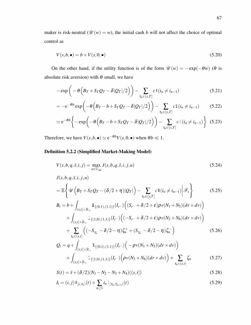
67
maker is risk-neutral (U (w) = w), the initial cash b will not affect the choice of optimal
control as
V (s,b,•) = b+V (s,0,•) (5.20)
On the other hand, if the utility function is of the form U (w) = −exp(−θw) (θ is
absolute risk aversion) with θ small, we have
−exp(−θ
(BT +ST QT −δ |QT |/2
))− ∑
τn∈(s,T ]c1(in 6= in−1) (5.21)
=−e−θb exp(−θ
(BT −b+ST QT −δ |QT |/2
))− ∑
τn∈(s,T ]c1(in 6= in−1) (5.22)
' e−θb−exp
(−θ
(BT −b+ST QT −δ |QT |/2
))− ∑
τn∈(s,T ]c1(in 6= in−1)
(5.23)
Therefore, we have V (s,b,•)' e−θbV (s,0,•) when θb 1.
Definition 5.2.2 (Simplified Market-Making Model)
V (s,b,q, s, i, j) = maxu∈Uad
J(s,b,q, s, i, j,u) (5.24)
J(s,b,q, s, i, j,u)
= E
U(
BT +ST QT − (δ/2+η)|QT |)− ∑
τn∈(s,T ]c1(in 6= in−1)
∣∣∣∣Fs
(5.25)
Bt = b+∫(s,t]×R+
1(0,1),(1,1)(Ir−)((Sr−+δ/2+ ε)ρv(N1 +N5)(dr×dv)
)+∫(s,t]×R+
1(1,0),(1,1)(Ir−)((−Sr−+δ/2+ ε)ρv(N2 +N6)(dr×dv)
)+ ∑
τn∈(s,t]
((−S
τ−n−δ/2−η)ζ+
n +(Sτ−n−δ/2−η)ζ−n
)(5.26)
Qt = q+∫(s,t]×R+
1(0,1),(1,1)(Ir−)(−ρv(N1 +N5)(dr×dv)
)+∫(s,t]×R+
1(1,0),(1,1)(Ir−)(
ρv(N2 +N6)(dr×dv))+ ∑
τn∈(s,t]ζn (5.27)
S(t) = s+(δ/2)(N1−N2−N3 +N4)((s, t]) (5.28)
It = (i, j)1[s,τ1)(t)+ ∑n≥1
in1[τn,τn+1)(t) (5.29)

68
λi(t) = λi(s)+∫ t
sβi(µi−λi(t))dt +
6
∑j=1
∫[s,t)
αi jdN j(t) i = 1, ...,6 (5.30)
5.3 Solving the Optimal Control Problem
The stochastic optimal control problem can be solved via constrained forward backward
stochastic differential equation (CFBSDE) as in Section A.4 and we state the representation
for the simplified model 5.2.2 here.
Theorem 5.3.1 The value function V of the simplified market-making model 5.2.2 is given
by V (s,b,q, s, i, j) = Ys where (Y,U,U ′,K) ∈ S2×L2N ×L2
N′ ×A2 is the unique minimal
solution of the following CFBSDE.
Bt = b+∫(s,t]×R+
1(0,1),(1,1)(Ir−)((Sr−+δ/2+ ε)ρv(N1 +N5)(dr×dv)
)+∫(s,t]×R+
1(1,0),(1,1)(Ir−)((−Sr−+δ/2+ ε)ρv(N2 +N6)(dr×dv)
)+∫(s,t]×I×J
((−Sr−−δ/2−η)ζ++(Sr−−δ/2−η)ζ−
)N′(dr×di×dζ ) (5.31)
Qt = q+∫(s,t]×R+
1(0,1),(1,1)(Ir−)(−ρv(N1 +N5)(dr×dv)
)+∫(s,t]×R+
1(1,0),(1,1)(Ir−)(
ρv(N2 +N6)(dr×dv))
+∫(s,t]×I×J
ζ N′(dr×di×dζ ) (5.32)
S(t) = s+(δ/2)(N1−N2−N3 +N4)((s, t]) (5.33)
It = (i, j)+∫(s,t]×I×J
(i− Ir−)N′(dr×di×dζ ) (5.34)
λi(t) = µi +∫ t
sβi(µi−λi(t))dt +
6
∑j=1
∫[s,t)
αi jdN j(t) i = 1, ...,6 (5.35)
Yt = U(
BT +ST QT −δ |QT |/2)−
d
∑j=1
∫(t,T ]×R+
U j(r,v)N j(dr×dv)
−∫(t,T ]×I×J
U ′(r, i,ζ )N′(dr×di×dζ )+KT −Kt (5.36)
U ′(t, i,ζ )≤ c ∀t ∈ (s,T ] (5.37)
Proof By theorem A.4.1 and A.4.2.

69
6. CONCLUSION
6.1 Summary of Contributions
• A new joint model of price and order arrivals is proposed and it has following fea-
tures:
– Prices and order arrivals are dependent via two linkages: common components
and cross-excitations of the underlying marked point processes.
– Prices are pure-jump processes living on a pre-defined price grid.
– Price jumps at the exact instant of aggressive order.
– The underlying processes driving the price movements are directly observable
and thus can be estimated using simple statistical methods.
– The order arrivals exhibit self- and cross-excitation behavior. Hawkes process
is used as an example but any marked point process with stochastic intensity is
compatible with our framework.
• The framework of solving optimal switching [28] and impulse control [27] by CFB-
SDE is extended in two ways
– The state variables can include marked point processes with stochastic intensi-
ties.
– The switching and impulse can occur at the same time.
• A new market-making model is put forward, which incorporate the enhancements
below:
– Prices and order arrivals are modeled using our new joint model.
– The quotes of market maker are switched in a discrete manner rather than con-
tinuously as in [9].

70
– The hard-to-estimate demand/supply rate function is no longer needed as the
market maker will either peg to the best quotes or withdraw from the market
similar to [12].
– Order volume is modeled by the random mark of the arrival point process.
– Market order is allowed as in [12] and it can be executed at the same time as
the quote switching.
– The stochastic control problem can be solved via Monte Carlo regression of
CFBSDE, which is more efficient than finite difference for state variables of
high dimension.
6.2 Future Works
Our new market-making model represents only the first attempt to provide a sensible
framework for real-world trading and it is definitely far from complete. In fact, it may
signify the start, rather than the end, of new series of research to be conducted under the
new structure of dependent price and arrivals in a pure-jump environment.
6.2.1 Point Process Modeling
From the result of the numerical experiment, a simple Markovian exponential kernel
seems not good enough to describe the subtle nature of high-frequency data. A thorough
examination of different types of kernels, such as power kernel [43], double exponential
[22] and Laguerre-type polynomial [44], in addition to a systematic study on the effect of
volume on excitation, is needed to improve the explanatory power of the model. Besides,
the non-linear Hawkes process (3.8) [48] have been developed for quite some time but its
use has been very limited. It will be very interesting to see if such sophistication can help
to portray the data more faithfully.

71
6.2.2 Portfolio Extension and Dimension Reduction
A natural progression for the joint price and order model is to extend it to multiple
assets. In a straight-forward manner, we can build a Hawkes process with n× d variates.
However, if we take the S&P 500 index with d = 6 and use the Markovian exponential
kernel, just the αi j matrix will have 9 million entries! Undoubtedly some kinds of di-
mension reduction techniques are needed. One way is to model dimensions as nodes,
cross-excitations as links between nodes and use graphical model to express the sparse
dependency structure [139].
The multi-asset joint model can help to develop a market-making strategy for portfolio
which explores the correlation structure across multiple assets. For example, if the inven-
tory of a market maker is +$1,000,000 of A and −$1,000,000 of B, his risk may not so
high if the prices of A and B are highly correlated. However, a single asset model may
opt for a suboptimal decision to reduce the seemingly excessive risk by liquidating both
inventory on A and B.
6.2.3 Queue Modeling
In our model, the penalization cost is simply a constant c and it is of course far from
satisfactory. The true cost of switching depends on how the limit orders are distributed
within the order book, which in turn depends on the strategy that the market maker uses to
secure the target order flow.
If the market maker has the subscription to the data feed from the exchange, he may be
able to compute the queue positions of his limit orders in real-time [140]. Armed with such
information, if we can develop a framework which estimates the intrinsic value of an array
of queue positions, the market-making model can adjust the switching decision based on
this dynamic switching cost.

72
6.2.4 Numerical Methods
The numerical methods to solve CFBSDE are still in their infancy. As see in the numeri-
cal examples, the numerical schemes are slow to converge and memory-intensive. Besides,
they become numerically unstable when penalization is used and the accuracy is further
deteriorates for point process with volatile marks.
Moreover the majority of the research effort concentrates on equation driven by Brown-
ian motion and we have not seen any numerical method specifically designed for pure-jump
process with stochastic intensity.
In addition, we would like to mention there are some numerical methods involving
Malliavin calculus [141] but they cannot be used in our framework as there is not yet a
version of Malliavin calculus for point process with stochastic intensity.
6.2.5 Adverse Selection
Since the market maker gives free options to all market participants in order to earn the
spread, he will always lose to informed traders. Adverse selection [1, 2] is a well-known
issue in market making. One way to minimize the loss is to temporarily withdraw from the
market if the market maker detects the heavy trading of insiders.
The Volume-synchronized Probability of Informed Trading (VPIN) [142, 143] is one
such measure, but more work is needed to see how we can incorporate this signal into the
control problem and backtest its performance on real-world trading.
6.3 Conclusion
In this thesis, we develop a new market-making model that try to incorporate a number
of realistic assumptions relevant for high-frequency trading. The job is tough and our result
is far from perfect. We have discussed some potential future works and we wish our initial
study will attract the attention of other researchers to work on this intriguing problem.

APPENDIX

73
Appendix: Control Problem and CFBSDE
A.1 Introduction
Assuming the evolution of state Xt depends on the regime It , at each user chosen event
time τn we can either change the regime from in−1 to in or fire an impulse ζn, which causes
Xt to change by Γ(τn,Xτ−n,ζn). Our objective is to find a sequence of switches and impulses
(τn, in,ζn) so as to maximize the sum of terminal value g(T,XT , IT ) and running gain∫ Ts f (t,Xt , It)dt subject to the switching cost h1(•) and impulse cost h2(•). Such kind of
optimization problem (A.1-A.3) is called optimal switching and impulse control problem.
V (s,x, i) = maxτn,in,ζn
E(
g(T,XT , IT )+∫ T
sf (t,Xt , It)dt
− ∑τn∈(s,T ]
(h1(τn,Xτn−, in−1, in)+h2(τn,Xτn−,ζn)
)∣∣∣∣Fs
)(A.1)
Xt = x+∫ t
sb(r,Xr, Ir)dr+
∫(s,t]×K
γ(r,Xr−, Ir−,k)N(dr×dk)
+ ∑τn∈(s,t]
Γ(τn,Xτ−n,ζn) (A.2)
It = i1[s,τ1)(t)+∞
∑n=1
in1[τn,τn+1)(t) (A.3)
If the intensity λ (t) of the marked point process N(dt,dk) is deterministic, the value
function V is the viscosity solution [24] of the Hamilton-Jacobi-Bellman quasi-variational
inequality (HJBQVI) (A.4-A.5) [25, 26].
max
f (t,x, i)+Vt(t,x, i)+Vx(t,x, i)>b(t,x, i)
+∫K
(V (t,x+ γ(t,x, i,k), i)−V (t,x, i)
)λ (t)µ(t,dk),
maxjV (t,x, j)−h1(t,x, i, j)−V (t,x, i),
maxζ
V (t,x+Γ(t,x,ζ ), i)−h2(t,x,ζ )−V (t,x, i)= 0 (A.4)
V (T,x, i) = g(T,x, i) (A.5)

74
However, when the intensity λ (t) is stochastic but we still apply the same method naively,
the resulting optimality condition will become a partial integro-differential equation (PIDE)
with random coefficients. Even if we can solve the PIDE for each ω , the solution will not
equal the value function of the control problem as the value function is non-random.
The trouble lies on the fact that the intensity now contains information about the current
state of the system. Suppose the intensity λt is bounded below, there exists a Girsanov
change of measure [55] such that under some equivalent probability measure Q, N is a
marked Poisson process. The stochastic intensity λ (•) will appear in the Girsanov kernel
Lt when we compute the value function under Q.
dQdP
= Lt (A.6)
Lt = exp(∫
(0,t]− log(λ (r))N(dr)+
∫(0,t]×K
(λ (r)−1)µ(r,dk)dr)
(A.7)
V (s,x, i)
= maxτn,in,ζn
EP(
g(T,XT , IT )+∫ T
sf (t,Xt , It)dt
− ∑τn∈(s,T ]
(h1(τn,Xτn−, in−1, in)+h2(τn,Xτn−,ζn)
)∣∣∣∣Fs
)(A.8)
= maxτn,in,ζn
Ls EQ(
g(T,XT , IT )/LT +∫ T
sf (t,Xt , It)/LT dt
− ∑τn∈(s,T ]
(h1(τn,Xτn−, in−1, in)/LT +h2(τn,Xτn−,ζn)/LT
)∣∣∣∣Fs
)(A.9)
However, after the change of measure, the control problem is no longer in the standard form
that can be solved by HJBQVI as the driver f and cost h1,h2 involve a random quantity
measurable at the terminal time T .
Regular stochastic optimal control problem can be solved via stochastic maximum prin-
ciple which describes the optimality condition in the form of a backward stochastic differ-
ential equation (BSDE) [144]. However, it is not until 20101 that Kharroubi et al. [27]
establish the connection of constrained forward backward stochastic differential equation
1Peng and Xu [145] (2007) also discuss the connection of CBSDE with QVI but the paper remains unpub-lished as of Apr 2015.

75
(CFBSDE) to impulse control problem. Later in 20142, Elie and Kharroubi [28] apply
CFBSDE to solve optimal switching.
While Kharroubi et al. [27], Elie and Kharroubi [28] focus on state variable driven
by Brownian motion, we have extended the formulation to include state variable driven
by marked point process with stochastic intensity and enrich the framework to handle the
combined optimal switching and impulse control problem, where switching and impulse
can happen at the same time.
Unlike HJBQVI, the structure of CFBSDE is by design random, hence the stochastic
intensity does not add much complexity to the system. Moreover, the CFBSDE can be
solved via Monte Carlo simulation, which is much more efficient than finite difference
when the dimension of Xt is high.
A nice introduction of impulse control with jumps can be found in [26] and the classic
reference for HJBQVI is [146]. For an excellent introduction of FBSDE with jumps and
CFBSDE, readers can refer to [147] and [27, 28, 148, 149] respectively.
A.2 Notation
Let T > 0 be a fixed terminal time and (Ω,F ,P) be a complete probability space en-
dowed with a d-variate simple marked point process (MPP) N on [0,T ]×K, as well as
another MPP N′ on [0,T ]× I× J where K is the mark space of N and I,J are respec-
tively the regime and impulse space. I,J,K are subsets of Euclidean space and N,N′ are
independent from each others. Ft denotes the augmented right-continuous filtration
generated by N,N′ and P is the predictable σ -field. Each variate of N is assumed to
have an absolutely continuous compensator in the form of λ j(t)µ j(t,dk)dt where λ j(t)
is the stochastic intensity, µ j(t,dk) is the conditional mark distribution and N j(dt,dk) =
N j(dt,dk)−λ j(t)µ j(t,dk)dt is the compensated marked point process. N′ is assumed to a
marked Poisson process with intensity λ ′.
2Though the paper was published in 2014, the preprint appeared in 2009.

76
The dimensions of various functions to be used in the coming sections are specified
here.
b : [0,T ]×Rn× I−→ Rn, γ j : [0,T ]×Rn× I×K−→ Rn (A.10)
f : [0,T ]×Rn× I−→ R, g : [0,T ]×Rn× I−→ R (A.11)
h1 : [0,T ]×Rn× I2 −→ R+, h2 : [0,T ]×Rn×J−→ R+ (A.12)
Γ : [0,T ]×Rn×J−→ Rn (A.13)
We also define a few standard function spaces and their norms for the ease of exposition.
S2 =
Y : Ω× [0,T ]−→ R
∣∣∣∣Yt ∈Ft , càdlàg, E(
supt∈[0,T ]
|Yt |2)< ∞)
(A.14)
‖Y‖2S2 = E
(sup
t∈[0,T ]|Yt |2
)(A.15)
A2 =
K ∈ S2
∣∣∣∣Kt is non-decreasing a.s., K0 = 0
(A.16)
L2N =
U : Ω× [0,T ]×K−→ Rd
∣∣∣∣U(•,k) ∈P,
E( d
∑j=1
∫ T
0
∫K|U j(t,k)|2λ j(t)µ j(t,dk)dt
)< ∞)
(A.17)
‖U‖2L2
N= E
( d
∑j=1
∫ T
0
∫K|U j(t,k)|2λ j(t)µ j(t,dk)dt
)(A.18)
A.3 Problem Formulation
The combined optimal switching and impulse control problem consists of finding a se-
quence of stopping time to switch the regime of the state Xt in order to change its dynamics
and/or to initiate an impulse which change the value of Xt immediately. We extend the
setting in [25] where the state is driven by a Brownian motion and the optimal switching
and impulse control is triggered one at a time. When the state is a diffusion, usually one of
the switching or impulse triggering boundaries will be hit before the other, so this setting
is appropriate.
However, in our case of pure-jump process, a large jump may push the state far out
of the optimal region and it may be optimal to switch regime and fire impulse right af-

77
ter this large jump. Considering only one action at a time may lead to suboptimal result.
For example, suppose the impulse is costly but can create immediate impact on the state,
the one-at-a-time setting may choose to trigger only a large impulse while the simultane-
ous setting may opt for a switch to a defensive regime together with a smaller impulse.
Anyways, since the simultaneous setting will consider switching only, impulse only and
switching + impulse, the result will always outperform the one-at-a-time framework.
The switching and impulse are assumed to be activated shortly3 after the uncontrolled
jump N, so the new regime i and impulse strength ζ can depend on the state after the uncon-
trolled jump. An impulse at time τ with strength ζ will advance the state by Γ(τ,Xτ−,ζ )
where Xτ− is the state just before time τ . It is the active regime at time t after the switching.
To simplify the model, we assume that the impulse transformation Γ does not depend on the
regime; otherwise we need to take into consideration the order of switching and impulse.
The dynamics of the state variable and regime can be written as follows.
Xt = y+∫ t
sb(r,Xr, Ir)dr+
d
∑j=1
∫(s,t]×K
γ j(r,Xr−, Ir−,k)N j(dr×dk)
+ ∑τn∈(s,t]
Γ(τn,Xτ−n,ζn) (A.19)
It = i1[s,τ1)(t)+ ∑n≥1
in1[τn,τn+1)(t) (A.20)
We impose the following standard Lipschitz and linear growth assumptions to ensure
the existence and regularity of the solution of the (forward) SDE.
Assumption A.3.1
‖b(t,x, i)−b(t,x′, i)‖+d
∑j=1
∫K‖γ j(t,x, i,k)− γ j(t,x′, i,k)‖λ j(t)µ j(t,dk)
+ supζ∈J‖Γ(t,x,ζ )−Γ(t,x′,ζ )‖ ≤C‖x− x′‖ a.s. (A.21)
‖b(t,x, i)‖+d
∑j=1
∫K‖γ j(t,x, i,k)‖λ j(t)µ j(t,dk)
+ supζ∈J‖Γ(t,x,ζ )‖ ≤C(1+‖x‖) a.s. (A.22)
3For technical reason, we assume the switching and impulse cannot occur at the same time as the uncontrolledjump N.

78
A control u = (τn, in,ζn)n≥1 consists of an increasing sequence of F -stopping time
τn, new regime in ∈ I = 1, ...,R and impulse strength ζn ∈ J = C∪ ∅,C compact.
in = in−1 means no switching while ζn =∅ indicates no impulse.
There is a technical condition that the control time τn cannot coincide with the jump
time of the point processes N j as we will later use change of measure to change the
intensity of point process associated with the control. Without this technical condition, the
other point processes will also be affect by this change of measure. In practice, there is
always a non-zero processing time, so the switching and impulse will never happen right
after the order arrivals.
The control problem is to find the optimal decision u such that the value function
V (s,y, i), composed of the terminal gain g, running gain f minus the switching cost h1
and impulse cost h2, is maximized. We define h = h1+h2 in order to simplify the notation.
X s,y,it stands for value of X at time t starting with Xs = y and Is = i but we will omit the
superscript if the meaning is clear.
V (s,y, i) = supu∈Uad
E(
g(T,X s,y,iT , Is,y,i
T )+∫ T
sf (t,X s,y,i
t , Is,y,it )dt
− ∑τn∈(s,T ]
h(τn,Xs,y,iτ−n
, Is,y,iτ−n, in,ζn)
∣∣∣∣Fs
)(A.23)
Uad =
(τn, in,ζn) ∈ R+× I×J|τn are Ft stopping times,
s < τn < τn+1 ≤ T, in ∈Fτ−n, ζn ∈F
τ−n, in 6= in−1 or ζn 6=∅,
|τn−σn, j| ≥ ε ∀n, j where σn, j is nth jump of N j
(A.24)
h(t,x, i, j,ζ ) = h1(t,x, i, j)+h2(t,x,ζ ) (A.25)
The following set of assumption makes sure the control problem is well-posed. The
Lipschitz and linear growth conditions of f ,g,h1,h2 (A.26-A.27) ensure that the value
function is well-defined. The strict sublinearity conditions of h1,h2 (A.28-A.29) remove
the possibility of consecutive switches or impulses. The lower bounds of h1,h2 (A.30-
A.31) guarantee that the optimal control is a finite sequence. (A.32) mandates that there
is no switching or impulse at the terminal time T so as to simplify the terminal condition.

79
Finally, (A.33-A.34) require that γ j are predictable and Γ,h1,h2 are left-continuous so that
the stochastic integrals with respect to point processes are well-defined.
Assumption A.3.2
| f (t,x, i)− f (t,x′, i)|+ |g(t,x, i)−g(t,x′, i)|
+|h1(t,x, i, j)−h1(t,x′, i, j)|+ |h2(t,x,ζ )−h2(t,x′,ζ )| ≤C‖x− x′‖ (A.26)
f (t,x, i)≤C(1+‖x‖), g(t,x, i)≤C(1+‖x‖), h(t,x, i, j,ζ )≤C(1+‖x‖) (A.27)
h1(t,x, i,k)+C ≤ h1(t,x, i, j)+h1(t,x, j,k) ∃C > 0 (A.28)
h2(t,x,ζ +ζ′)+C ≤ h2(t,x,ζ )+h2(t,x,ζ ′) ∃C > 0 (A.29)
h1(t,x, i, i) = 0, h1(t,x, i, j)≥C ∃C > 0 ∀i 6= j (A.30)
h2(t,x,∅) = 0, h2(t,x,ζ )≥C ∃C > 0 ∀ζ 6=∅ (A.31)
g(T,x, i)≥ supj∈I,ζ∈J
g(T,x+ζ , j)−h1(T,x, i, j)−h2(T,x,ζ ) (A.32)
γ j ∈P, Γ(t,x,ζ ) = Γ(t−,x,ζ ) (A.33)
h1(t,x, i, j) = h2(t−,x, i, j), h2(t,x,ζ ) = h2(t−,x,ζ ) (A.34)
A.4 Solution via CFBSDE
The following constrained forward backward stochastic differential equation (CFB-
SDE) is the key to finding the value function V (s,y, i) of the optimal control problem.
Since the forward (A.35-A.36) and backward (A.37-A.38) equations are uncoupled (for-
ward equation does not depend on (Y,U,U ′,K)), the forward equation can be solved sep-
arately using classical methods. Hence our focus will be on the constrained backward
equation.
Xt = Xs +∫ t
sb(r,Xr, Ir)dr+
d
∑j=1
∫(s,t]×K
γ j(r,Xr−, Ir−,k)N j(dr×dk)
+∫(s,t]×I×J
Γ(r,Xr−,ζ )N′(dr×di×dζ ) (A.35)
It = Is +∫(s,t]×I×J
(i− Ir−)N′(dr×di×dζ ) (A.36)

80
Yt = g(T,XT , IT )+∫ T
tf (r,Xr, Ir)dr−
d
∑j=1
∫(t,T ]×K
U j(r,k)N j(dr×dk)
−∫(t,T ]×I×J
U ′(r, i,ζ )N′(dr×di×dζ )+KT −Kt (A.37)
U ′(t, i,ζ )≤ h(t,Xt−, It−, i,ζ ) ∀t ∈ (s,T ] (A.38)
In the CBSDE, N′(dt×di×dζ ) is the marked point process associated with the control
but it can be chosen to have any distribution provided that the intensity of N′ is strictly
positive and the support of the conditional mark distribution of N′ is the whole mark space
I×J. For the ease of computation, N′ is usually taken to be a Poisson process independent
from N. Such a feature is called control randomization in [150] and in the proof of theorem
A.4.2, you can see that it is a result of change of probability measure.
As its name implied, the solution component U ′ of the CBSDE must be less than h at
all time between s and T . It is this restriction that force the component Y to equal to the
value function V of the associated control problem.
The following condition gives a way to check if the CBSDE (A.37-A.38) is well-posed.
Theorem A.4.1 If f (t,x, i)≤C(1+‖x‖), g(t,x, i)≤C(1+‖x‖), 0≤ h(t,x, i, j,ζ )≤C(1+
‖x‖), then the CBSDE (A.37-A.38) admits a solution.
Proof Let
U j(t,k) = 0, U ′(t, i,ζ ) = h(t,Xt−, It−, i,ζ ) (A.39)
Kt =
∫ t
0
(C(1+‖Xr‖)− f (r,Xr, Ir)
)dr
+∫(0,t]×I×J
h(r,Xr−, Ir−, i,ζ )N′(dr×di×dζ ) t ∈ [0,T )
KT−+C(1+‖XT‖)−g(T,XT , IT ) t = T
(A.40)
Yt =
C(1+‖XT‖)+
∫ T
tC(1+‖Xr‖)dr t ∈ [0,T )
g(T,XT , IT ) t = T(A.41)
By construction (Y,U,U ′,K) satisfies the equation (A.37-A.38). From the given condition,
Kt is non-decreasing. Using X ∈ S2, Jensen’s and other simple inequalities, we get
E(
supt∈[0,T ]
|Yt |2)
(A.42)

81
≤ E(
supt∈[0,T ]
(C(1+‖XT‖)+
∫ T
tC(1+‖Xr‖)dr+g(T,XT , IT )
)2)
(A.43)
≤ E(
supt∈[0,T ]
3(
C2(1+‖XT‖)2 +∫ T
tC2(1+‖Xr‖)2dr+g2(T,XT , IT )
))(A.44)
≤ E(
supt∈[0,T ]
3(
2C2(1+‖XT‖)2 +∫ T
0C2(1+‖Xr‖)2dr
))(A.45)
≤ E(
supt∈[0,T ]
3(
4C2(1+‖XT‖2)+2TC2(1+‖Xt‖2)))
(A.46)
≤ E(
12C2(1+ supt∈[0,T ]
‖Xt‖2)+6TC2(1+ supt∈[0,T ]
‖Xt‖2)
)≤ ∞ (A.47)
E(
supt∈[0,T ]
|Kt |2)= E(|KT |2) (A.48)
≤ 4E(∫ T
0
(C(1+‖Xr‖)− f (r,Xr, Ir)
)2dr+C2(1+‖XT‖)2 +g2(T,XT , IT )
+∫(0,T ]×I×J
h2(r,Xr−, Ir−, i,ζ )N′(dr×di×dζ )
)(A.49)
≤ 4E(∫ T
04(
C2(1+‖Xr‖)2)
dr+C2(1+‖XT‖)2 +C2(1+‖XT‖)2
+∫(0,T ]×I×J
C2(1+‖Xr‖)2λ′µ′(r,di×dζ )dr
)(A.50)
≤ 4E(∫ T
08(
C2(1+‖Xr‖2))
dr+4C2(1+‖XT‖2)
+∫(0,T ]×I×J
2C2(1+‖Xr‖2)λ ′µ ′(r,di×dζ )dr)
(A.51)
≤ 4E(
8TC2(1+ supt∈[0,T ]
‖Xt‖2)+4C2(1+ supt∈[0,T ]
‖Xt‖2)
+2T λ′C2(1+ sup
t∈[0,T ]‖Xt‖2)
)≤ ∞ (A.52)
E(∫ T
0
∫K|U ′(t, i,ζ )|2λ
′µ′(t,di×dζ )dt
)(A.53)
= E(∫ T
0
∫K|h′(t,Xt−, It−, i,ζ )|2λ
′µ′(r,di×dζ )dt
)(A.54)
≤ E(∫ T
0
∫K
C2(1+‖Xt‖)2λ′µ′(t,di×dζ )dt
)(A.55)
≤ E(
2C2λ′T (1+ sup
t∈[0,T ]‖Xt‖2)
)≤ ∞ (A.56)
Thus (Y,U,U ′,K) ∈ S2×L2N×L2
N′×A2

82
The following theorem is the main result of this section.
Theorem A.4.2 If assumptions (A.3.1), (A.3.2) hold and there exists a solution to the CB-
SDE (A.37-A.38), then there exists an unique minimal solution4 (Y,U,U ′,K) ∈ S2×L2N×
L2N′×A2 with K predictable.
Moreover, if (Y,U,U ′,K) ∈ S2×L2N ×L2
N′ ×A2 is a minimal solution of (A.37-A.38),
then
V (s,y, i) = Y s,y,is ∀s ∈ [0,T ] (A.57)
and the optimal control is
τn = inf
t > τn−1∣∣V (t,X s,y,i
t− , Is,y,it− ) =V (t,X s,y,i
t− +Γ(t,X s,y,it− ,ζ ), j)
−h(t,X s,y,it− , Is,y,i
t− , j,ζ ) for some j 6= It− or ζ 6=∅
(A.58)
(in,ζn) = argmaxj∈I,ζ∈J
V (τn,X
s,y,iτ−n
+Γ(τn,Xs,y,iτ−n
,ζ ), j)−h(τn,Xs,y,iτ−n
, Is,y,iτ−n, j,ζ )
(A.59)
Proof Let V be the set of bounded predictable random field ν(t, i,ζ ) on [0,T ]× I×J and
we define Lt and the probability measure Pν as
dLt = Lt−
∫I×J
(ν(t, i,ζ )−1)N′(dt×di×dζ ), L0 = 1 (A.60)
Pν(A) =∫
ALtdP (A.61)
Eν denotes the expectation under Pν . By Girsanov theorem for marked point process
[55], the compensator measure of N′ changes from λ ′µ ′(t,di×dζ )dt in P to
ν(t, i,ζ )λ ′µ ′(t,di×dζ )dt (A.62)
in Pν . Noticing that the value function has another representation.
Vt = supν∈V
Eν
(g(T,XT , IT )+
∫ T
tf (r,Xr, Ir)dr
−∫(t,T ]×I×J
h(r,Xr−, Ir−, i,ζ )N′(dr×di×dζ )
∣∣∣∣Ft
)(A.63)
4Yt is called a minimal solution if Yt is a solution and Yt ≤ Yt for all solution Yt .

83
Let (Y,U,U ′,K) ∈ S2×L2N ×L2
N′ ×A2 be any solution of the CBSDE (A.37-A.38).
Taking the essential supremum of conditional expectation under Pν on Yt (A.37) (N is not
affected by the change of measure), we have
Yt = supν∈V
Eν
(g(T,XT , IT )+
∫ T
tf (r,Xr, Ir)dr
−∫(t,T ]×I×J
U ′(r, i,ζ )N′(dr×di×dζ )+KT −Kt
∣∣∣∣Ft
) (A.64)
≥ supν∈V
Eν
(g(T,XT , IT )+
∫ T
tf (r,Xr, Ir)dr
−∫(t,T ]×I×J
h(r,Xr−, Ir−, i,ζ )N′(dr×di×dζ )
∣∣∣∣Ft
) (A.65)
=Vt (A.66)
Conversely, it can well-known that
Qt = supν∈V
Eν
(g(T,XT , IT )+
∫ T
0f (r,Xr, Ir)dr
−∫(0,T ]×I×J
h(r,Xr−, Ir−, i,ζ )N′(dr×di×dζ )
∣∣∣∣Ft
) (A.67)
=Vt +∫ t
0f (r,Xr, Ir)dr−
∫(0,t]×I×J
h(r,Xr−, Ir−, i,ζ )N′(dr×di×dζ ) (A.68)
is a càdlàg Pν -supermartingale ∀ν ∈V (see [151, proposition 4.2] or [152, theorem 2.1.1]).
Since Vt ≤ Yt ∈ S2 and f (t,x, i),h(t,x, i, j,ζ ) grows sublinearly with x, we can see that
Q ∈ S2. Take ν(t, i,ζ ) = 0 and by Doob-Meyer decomposition under P0,
Qt =V0 +M0t −K0
t (A.69)
where M0t is a càdlàg P0-martingale with M0
0 = 0 and K0t is a càdlàg, predictable and in-
creasing process with K00 = 0. Since Q ∈ S2, we have M0 ∈ S2 and K0 ∈A2. By martingale
representation theorem, we can express M0t in N j and N′0. However, when ν(t, i,ζ ) = 0,
N′ν(dt×di×dζ ) = 0. As M0 ∈ S2, there exists U j ∈ L2N such that
Qt =V0 +d
∑j=1
∫(0,t]×K
U j(r,k)N j(dr×dk)−K0t (A.70)

84
Substitute Qt in (A.68)
Vt = g(T,XT , IT )+∫ T
tf (r,Xr, Ir)dr−
d
∑j=1
∫(t,T ]×K
U j(r,k)N j(dr×dk)
−∫(t,T ]×I×J
h(r,Xr−, Ir−, i,ζ )N′(dr×di×dζ )+K0
T −K0t (A.71)
Hence (V,U,h,K0)∈ S2×L2N×L2
N′×A2 is a minimal solution of the CBSDE (A.37-A.38).
Y is unique by definition of minimal solution. The uniqueness of (U,U ′,K) follows by
identifying the predictable and totally inaccessible parts as well as from the fact that N and
N′ have no common jump.
A.5 Numerical Scheme
One way to solve the CFBSDE (A.35-A.38) is via solving the associated penalized
(unconstrained) FBSDE (A.72) which converges weakly to the CFBSDE as p−→ ∞ [27].
Yt = g(T,XT , IT )+∫ T
tfp(r,Xr, Ir,U ′(r,•))dr−
d
∑j=1
∫(t,T ]×K
U j(r,k)N j(dr×dk)
−∫(t,T ]×I×J
U ′(r, i,ζ )N′(dr×di×dζ )
(A.72)
fp(r,Xr, Ir,U ′(r,•)) = f (r,Xr, Ir)
+∫I×J
(p(
U ′(r, i,ζ )−h(r,Xr, Ir, i,ζ ))+−U ′(r, i,ζ )
)λ′µ′(r,di×dζ ) (A.73)
Therefore, the methods for solving CFBSDE boil down to the ones for solving uncon-
strained FBSDE. We recommend using the forward scheme [153] but we will first discuss
the more intuitive backward scheme and its drawbacks.
For simplicity, we will assume the mark distributions of both N and N′ are non-random
and independent of time.

85
A.5.1 Backward Scheme
The period [0,T ] is divided into a time grid 0 = t0 < t1 < ... < tN = T of N5 uniform
intervals of length ∆t = T/N and M sample paths are generated. For simplicity, we denote
the value of X(tn) as Xn and the filtration Ftn as Fn.
We assume the forward equation is a pure-jump process, and it can be simulated ex-
actly without any discretization error. For details about simulation of multivariate marked
Hawkes process, please refer to Section 3.4.1.
It is easy to see that the backward equation can be approximated by
Yn = Yn+1 + fp(tn,Xn, In,U ′(tn,•))∆t−d
∑j=1
∫K
U j(tn,k)N j((tn, tn+1]×dk)
−∫I×J
U ′(tn, i,ζ )N′((tn, tn+1]×di×dζ ) (A.74)
Since the terminal value YN is known to be g(T,XN , IN), the backward equation can be
computed backward from time T . However, such a solution will not be adapted, so we
take conditional expectation given Fn. Since integral of N j is a martingale and fp does not
depend on U j, this relieves our burden to compute U j. Taking conditional expectation on
(A.74) given Fn, we get
Yn = E(Yn+1|Fn)+ fp(tn,Xn, In,U ′(tn,•))∆t (A.75)
U ′(tn, i,ζ ) is determined by discretizing the mark (i,ζ ) and then taking conditional ex-
pectation on (A.74) after multiplying the martingale N′((tn, tn+1], i,ζ ) to both side of the
equation (N′ and N j are independent).
U ′(tn, i,ζ ) =E(Yn+1N′((tn, tn+1], i,ζ )|Fn)
λ ′µ(i,ζ )∆t(A.76)
fp(tn,Xn, In,U ′(tn,•)) = f (tn,Xn, In)
+∑i,ζ
(p(
U ′(tn, i,ζ )−h(r,Xn, In, i,ζ ))+−U ′(tn, i,ζ )
)λ′µ′(i,ζ ) (A.77)
5We use the standard symbol N for the number of time steps and readers are reminded not to confuse withthe point process N, which will be denoted as N j(t).

86
Assuming Yn and U(tn, i,ζ ) do not depend on λ j(tn) (see Section 5.2.2), the conditional
expectation given Fn is simply the conditional expectation given Xn, In and it can be esti-
mated via Monte Carlo regression on a set of user chosen basis functions of size K with the
M generated sample paths as input data. For details, readers can refer to [154, 155].
In addition to the choice of basis functions, there are five parameters in the backward
scheme, namely p,λ ′,N,M,K, where p,λ ′ control the penalization error. As the uncon-
strained FBSDE converges to the CFBSDE when p−→ ∞, p needs to be reasonably large.
However, a large p will introduce numerically instability to the algorithm (see numerical
example 2). Also, if λ ′ is too small, there is simply no control event and U ′ will never
be penalized. When both λ ′ and p are large, the discretization error will increase and we
need a finer grid to better approximate fp and U ′ due to more frequent control events. For
Brownian motion, readers can refer to [156] for the formula of the error bound.
In the backward scheme, the output of the regression at tn+1 is used as an input for the
next regression at tn (nested regressions), so the error accumulates along the backward iter-
ation. When we increase the number of time steps N, the number of regressions increases
and so is the regression error. In order to keep the final error under control, we need to
increase the number of sample paths M and the number of basis functions K. For the case
of FBSDE drive by Brownian motion and using hypercube basis functions, Gobet [157]
has the following suggestion: M = O(N3+d), K = O(Nd) where d is the dimension of state
variable X . For example, when N = 103, d = 4, we have M = O(1021), K = O(1012),
which is clearly impractical.
A.5.2 Forward Scheme
In the so-called forward scheme [153], in each iteration, all the Yn, U ′nNn=0 are com-
puted at the same time using the following well-known Picard type iteration for BSDE.
Theorem A.5.1 If assumptions (A.3.1), (A.3.2) hold, then the solution (Y q+1,Uq+1,U ′q+1)
of the BSDE

87
Y q+1t = g(T,XT , IT )+
∫ T
tfp(r,Xr, Ir,U ′q(r,•))dr−
d
∑j=1
∫(t,T ]×K
Uq+1j (r,k)N j(dr×dk)
−∫(t,T ]×I×J
U ′q+1(r, i,ζ )N′ j(dr×di×dζ ) (A.78)
converges to the solution (Y,U,U ′) of the BSDE
Yt = g(T,XT , IT )+∫ T
tfp(r,Xr, Ir,U ′(r,•))dr−
d
∑j=1
∫(t,T ]×K
U j(r,k)N j(dr×dk)
−∫(t,T ]×I×J
U ′(r, i,ζ )N′ j(dr×di×dζ ) (A.79)
as q−→ ∞ in S2×L2N×L2
N′ .
Proof See [147, Theorem 3.1.1]
Formulae for (Y q+1n ,U ′q+1
n ) in the (q+ 1)th Picard iteration are derived using the
similar method as the backward scheme except (Y q+1n ,U ′q+1
n ) is calculated directly from
(g(T,XT , IT ),U ′q) in the previous Picard iteration instead of (Y q+1n+1 ,U
′q+1n+1) from the next
period.
U ′0n = 0 ∀n (A.80)
U ′q+1(tn, i,ζ ) =E((
g(T,XT , IT )+∑N−1k=n fp(tk,Xk, Ik,U ′q(tk,•))∆t
)N′((tn, tn+1], i,ζ )
∣∣∣Fn
)λ ′µ(i,ζ )∆t
(A.81)
fp(tn,Xn, In,U ′q+1(tn,•)) = f (tn,Xn, In)
+∑i,ζ
(p(U ′q+1(tn, i,ζ )−h(r,Xn, In, i,ζ )
)+−U ′q+1(tn, i,ζ ))
λ′µ′(i,ζ ) (A.82)
Y q+1n = E
(g(T,XT , IT )+
N−1
∑k=n
fp(tk,Xk, Ik,U ′q(tk,•))∆t∣∣∣Fn
)(A.83)
The conditional expectation is again computed using Monte Carlo regression [154, 155].
Compared with the backward scheme, which needs only one iteration to compute Y0,
the forward scheme need several iterations albeit the Picard iteration usually converges
very fast. However, the regressions at different times tn in the forward scheme can be
computed in parallel as the input is X , I and Uqn in the previous Picard iteration whereas

88
in the backward scheme, the regression at time tn depends on the regression result at time
tn+1.
The second and more important difference is that the regression error does not accumu-
late over time. In each regression, g(T,XT , IT ) can be simulated exactly in our pure-jump
model and U ′q will be close to the true U ′ when q is sufficiently large, so the regression
error will mostly depend on the choice of basis functions and the number of sample paths
M. Although the regression error will accumulate over Picard iterations, the number of
iterations required is usually very small.
In short, we can choose a relatively large p,λ ′ and N such that the penalization error
and discretization error is sufficiently small. Then the final error will only depend on the
goodness-of-fit of the worst regression. Since the regression error does not accumulate over
time, it will only depends on M,K and the choice of basis functions but not p,λ ′,N (see
[153] for error bound in the case of Brownian motion).
A.5.3 Numerical Examples
Example 1
Let Nt be a Poisson process with intensity λ . The solution of the following FBSDE
Xt = Nt (A.84)
Yt =(
XT +2X2T
)+∫ T
t
(exp(− (Ur− (3+4Xr))
2)−λUr
)dr−
∫ T
tUrdNr (A.85)
is given by Yt = (1− t)+Xt +2X2t , Ut = 3+4Xt− and in particular, Y0 = 1.
We solve the FBSDE numerically using forward scheme with hypercube basis of 10
intervals (K = 10) and 5 Picard iterations. Because of memory limitation6, we fix the num-
ber of time step N to 10 and use different values of λ to study the effect of discretization.
The values of Y0 for different intensities λ and numbers of sample paths M are shown in
Table A.1.6We already run our program on a special cluster of Purdue’s supercomputer Carter with 256G memory.

89
Table A.1.
Value of Y0 by solving the FBSDE (A.85) numerically with N = 10,K = 10and 5 Picard iterations. True Y0 = 1.
M \λ 0.01 0.1 1
104 0.6714 0.7848 0.5916105 0.7938 0.9253 0.6685106 0.8276 0.9962 0.6712107 0.8610 0.9969 0.6464
Although the regression error does not accumulate over time in the forward scheme, we
still needs more than a few million sample paths M in order to get a reasonable estimate
of Y0. On the other hand, as the intensity λ increases, the events arrive more often and we
need a finer grid in order to describe U(t) more accurately. From Table A.1, it seems that
we need something around N ' 100λT for the algorithm to converge. However, unlike the
case for M, larger N may not always mean better result in the pure-jump model. The reason
is that when the interval is too small relative to λ , there is simply no arrivals in most of the
intervals. More regressions just increase the volatility of U(t) and the rounding error when
we compute ∑N−1n=0 f (Xn,Un)∆t.
Example 2
In this example, we introduce a penalization term p(Ut − (3+ 4Xt))+ to the driver f ,
but since Ut = 3+4Xt− , the penalization term is indeed 0 and thus the solution is the same
as example 1.
Xt = Nt (A.86)
Yt =(
XT +2X2T
)−∫ T
tUrdNr
+∫ T
t
(p(Ur− (3+4Xr))
++ exp(−(Ur− (3+4Xr))
2)−λUr
)dr (A.87)
However, because of the discretization, regression and Picard iteration error, U(t) will
be larger than 3+ 4Xt− in some cases and a large p will cause the error to blow up (see

90
[156]) as shown in Table A.2. In this example, we fix N = 10,M = 107,λ = 0.1,T = 1 and
use 5 Picard iterations.
Table A.2.
Effect of penalization on the forward scheme with N = 10,M = 107,K =10,λ = 0.1,T = 1 and 5 Picard iterations. True Y0 = 1.
p 0.01 0.10 0.25 0.50 0.75 1.00
Y0 0.9972 0.9998 1.0058 1.1051 3.3716 14.6054
Example 3
In this example, we illustrate the effect of marks to the accuracy of the numerical solu-
tion.
Xt =∫(0,t]×K
kN(dr×dk) (A.88)
Yt = XT +∫ T
t
∫K
(exp(− (U(r,k)− k)2)−λU(r,k)
)µ(dk)dr
−∫(t,T ]×K
U(r,k)N(dr×dk) (A.89)
The solution of the FBSDE is Yt = (T − t) + Xt , U(t,k) = k for any mark distribution
µ(dk). Similar to previous cases, we fix N = 10,M = 107,λ = 0.1,T = 1 and use 5 Picard
iterations. The mark distribution µ(dk) is discrete uniform on 0,1C,2C, ..,9C with C =
1,10, ...,100000.
Table A.3.
Effect of marks on the forward scheme with N = 10,M = 107,K = 10,λ =0.1,T = 1 and 5 Picard iterations. True Y0 = 1.
C 1 10 100 1000 10000 100000
Y0(M = 107) 0.9715 0.8100 0.2389 -0.1308 -1.5024 -15.0239Y0(M = 108) 0.9967 0.8996 0.4324 0.0828 0.3829 3.8290

91
From Table A.3, we can see that the error increases as the marks become more volatile.
Moreover the computation time is 10 times longer as we need run a regression for each
value of k. Also the memory requirement drastically increases we need to hold more im-
mediate results during the Monte Carlo regression. The accuracy can be improved by
having more sample paths M but it will further aggravate the memory requirement and the
computational speed of the numerical scheme.

REFERENCES
92
REFERENCES
[1] L. Glosten and P. Milgrom. Bid, ask and transaction prices in a specialist marketwith heterogeneously informed traders. Journal of Fiancial Economics, 14(1):71–100, 1985.
[2] A. S. Kyle. Continuous auctions and insider trading. Econometrica, 53(6):1315,1985.
[3] Securities Exchange Commission. Concept release on equity market structure. Fed-eral Register, 75(13):3594–3614, 2010.
[4] The Board of the International Organization of Securities Commissions. Tradingfee models and their impact on trading behaviour. Technical report, InternationalOrganization of Securities Commissions, 2013.
[5] M. Garman. Market microstructure. Journal of Fiancial Economics, 3(3):257–275,1976.
[6] Y. Amihud and H. Mendelson. Dealership market: Market-making with inventory.Journal of Fiancial Economics, 8(1):31–53, 1980.
[7] H. Stoll. The supply of dealer services in securities markets. The Journal of Finance,33(4):1133–1151, 1978.
[8] T. Ho and H. Stoll. Optimal dealer pricing under transactions and return uncertainty.Journal of Fiancial Economics, 9(1):47–73, 1981.
[9] M. Avellaneda and S. Stoikov. High-frequency trading in a limit order book. Quan-titative Finance, 8(3):217–224, 2008.
[10] P. Fodra and M. Labadie. High-frequency market-making with inventory constraintsand directional bets. arXiv preprint arXiv:1206.4810, 2012.
[11] O. Guéant, C.-A. Lehalle, and J. Fernandez-Tapia. Dealing with the inventory risk:A solution to the market making problem. Mathematics and financial economics, 7(4):477–507, 2013.
[12] F. Guilbaud and H. Pham. Optimal high-frequency trading with limit and marketorders. Quantitative Finance, 13(1):79–94, 2013.
[13] P. Gopikrishnan, V. Plerou, X. Gabaix, and H. E. Stanley. Statistical properties ofshare volume traded in financial markets. Physical Review E, 62(4):R4493, 2000.
[14] S. Maslov and M. Mills. Price fluctuations from the order book perspec-tive—empirical facts and a simple model. Physica A: Statistical Mechanics andits Applications, 299(1):234–246, 2001.

93
[15] X. Gabaix, P. Gopikrishnan, V. Plerou, and H. E. Stanley. Institutional investors andstock market volatility. The Quarterly Journal of Economics, 121(2):461–504, 2006.
[16] P. Weber and B. Rosenow. Order book approach to price impact. QuantitativeFinance, 5(4):357–364, 2005.
[17] M. Potters and J.-P. Bouchaud. More statistical properties of order books and priceimpact. Physica A: Statistical Mechanics and its Applications, 324(1):133–140,2003.
[18] B. Biais, P. Hillion, and C. Spatt. An empirical analysis of the limit order book andthe order flow in the paris bourse. The Journal of Finance, 50(5):1655–1689, 1995.
[19] B. Tóth, I. Palit, F. Lillo, and J. D. Farmer. Why is order flow so persistent? arXivpreprint arXiv:1108.1632, 2011.
[20] J. Da Fonseca and R. Zaatour. Clustering and mean reversion in a Hawkes mi-crostructure model. Journal of Futures Markets, 2014.
[21] F. Pomponio and F. Abergel. Trade-throughs: Empirical facts and application tolead-lag measures, pages 3–16. Springer, 2011.
[22] J. Large. Measuring the resiliency of an electronic limit order book. Journal ofFinancial Markets, 10(1):1–25, 2007.
[23] E. Bacry, S. Delattre, M. Hoffmann, and J. F. Muzy. Some limit theorems for Hawkesprocesses and application to financial statistics. Stochastic Processes and their Ap-plications, 2013.
[24] M. G. Crandall and P.-L. Lions. Viscosity solutions of Hamilton-Jacobi equations.Transactions of the American Mathematical Society, 277(1):1–42, 1983.
[25] S. Tang and J. Yong. Finite horizon stochastic optimal switching and impulse con-trols with a viscosity solution approach. Stochastics: An International Journal ofProbability and Stochastic Processes, 45(3-4):145–176, 1993.
[26] B. K. Øksendal and A. Sulem. Applied stochastic control of jump diffusions.Springer, 2005.
[27] I. Kharroubi, J. Ma, H. Pham, and J. Zhang. Backward SDEs with constrained jumpsand quasi-variational inequalities. The Annals of Probability, 38(2):794–840, 2010.
[28] R. Elie and I. Kharroubi. BSDE representations for optimal switching problems withcontrolled volatility. Stochastics and Dynamics, 14(03), 2014.
[29] J.-P. Bouchaud, J. D. Farmer, and F. Lillo. How markets slowly digest changes insupply and demand. Handbook of financial markets: dynamics and evolution, 1:57,2009.
[30] R. Cont. Statistical modeling of high-frequency financial data. Signal ProcessingMagazine, IEEE, 28(5):16–25, 2011.
[31] A. Chakraborti, I. M. Toke, M. Patriarca, and F. Abergel. Econophysics review: I.empirical facts. Quantitative Finance, 11(7):991–1012, 2011.

94
[32] T. Andersen, T. Bollerslev, F. Diebold, and P. Labys. The distribution of realizedexchange rate volatility. Journal of the American Statistical Association, 96(453):42–55, 2001.
[33] O. E. Barndorff-Nielsen. Econometric analysis of realized volatility and its use inestimating stochastic volatility models. Journal of the Royal Statistical Society:Series B (Statistical Methodology), 64(2):253–280, 2002.
[34] O. Kallenberg. Random measures. Akademie-Verlag, 1983.
[35] A. Karr. Point processes and their statistical inference. CRC press, 1991.
[36] P. Brémaud. Point processes and queues. Springer, 1981.
[37] D. Daley and D. Vere-Jones. An introduction to the theory of point processes: Vol-ume I: Elementary theory and methods. Springer, 2003.
[38] D. Daley and D. Vere-Jones. An introduction to the theory of point processes: Vol-ume II: General theory and structure. Springer, 2007.
[39] F. Papangelou. The conditional intensity of general point processes and an applica-tion to line processes. Probability Theory and Related Fields, 28(3):207–226, 1974.
[40] P. A. Meyer. Démonstration simplifiée d’un théorème de knight. In Séminaire deprobabilités v université de strasbourg, pages 191–195. Springer, 1971.
[41] F. Papangelou. Integrability of expected increments of point processes and a relatedrandom change of scale. Transactions of the American Mathematical Society, 165:483–506, 1972.
[42] A. G. Hawkes. Spectra of some self-exciting and mutually exciting point processes.Biometrika, 58(1):83–90, 1971.
[43] Y. Ogata. Statistical models for earthquake occurrences and residual analysis forpoint processes. Journal of the American Statistical Association, 83(401):9–27,1988.
[44] Y. Ogata and H. Akaike. On linear intensity models for mixed doubly stochasticpoisson and self-exciting point processes. Journal of the Royal Statistical Society.Series B (Methodological), pages 102–107, 1982.
[45] D. Oakes. The markovian self-exciting process. Journal of Applied Probability,pages 69–77, 1975.
[46] A. G. Hawkes and D. Oakes. A cluster process representation of a self-excitingprocess. Journal of Applied Probability, pages 493–503, 1974.
[47] J. Møller and J. G. Rasmussen. Perfect simulation of Hawkes processes. Advancesin applied probability, pages 629–646, 2005.
[48] P. Brémaud and L. Massoulié. Stability of nonlinear Hawkes processes. The Annalsof Probability, pages 1563–1588, 1996.
[49] P. Brémaud, G. Nappo, and G. Torrisi. Rate of convergence to equilibrium of markedHawkes processes. Journal of Applied Probability, 39(1):123–136, 2002.

95
[50] C. G. Bowsher. Modelling security market events in continuous time: Intensitybased, multivariate point process models. Journal of Econometrics, 141(2):876–912, 2007.
[51] P. Brémaud and L. Massoulié. Hawkes branching point processes without ancestors.Journal of Applied Probability, 38(1):122–135, 2001.
[52] T. Jaisson and M. Rosenbaum. Limit theorems for nearly unstable Hawkes pro-cesses. arXiv preprint arXiv:1310.2033, 2013.
[53] L. Zhu. Central limit theorem for nonlinear Hawkes processes. Journal of AppliedProbability, 50(3):760–771, 2013.
[54] P. Billingsley. Convergence of probability measures. John Wiley & Sons, 2009.
[55] J. Jacod and A. N. Shiryaev. Limit theorems for stochastic processes. Springer-Verlag Berlin, 1987.
[56] T. Ozaki. Maximum likelihood estimation of Hawkes’ self-exciting point processes.Annals of the Institute of Statistical Mathematics, 31(1):145–155, 1979.
[57] Y. Ogata. On Lewis’ simulation method for point processes. Information Theory,IEEE Transactions on, 27(1):23–31, 1981.
[58] J. Zhuang, Y. Ogata, and D. Vere-Jones. Analyzing earthquake clustering features byusing stochastic reconstruction. Journal of Geophysical Research, 109(B5), 2004.
[59] P. A. Lewis and G. S. Shedler. Simulation of nonhomogeneous poisson processes bythinning. Naval Research Logistics Quarterly, 26(3):403–413, 1979.
[60] A. Veen and F. P. Schoenberg. Estimation of space–time branching process modelsin seismology using an EM–type algorithm. Journal of the American StatisticalAssociation, 103(482):614–624, 2008.
[61] A. P. Dempster, N. M. Laird, and D. B. Rubin. Maximum likelihood from incom-plete data via the EM algorithm. Journal of the Royal Statistical Society. Series B(Methodological), pages 1–38, 1977.
[62] G. Mclachlan and T. Krishnan. The EM algorithm and extensions. John Wiley &Sons, 2007.
[63] D. Marsan and O. Lengline. Extending earthquakes’ reach through cascading. Sci-ence, 319(5866):1076–1079, 2008.
[64] P. Halpin and P. Boeck. Modelling dyadic interaction with Hawkes processes. Psy-chometrika, 78(4):793–814, 2013.
[65] P. F. Halpin. A scalable EM algorithm for Hawkes processes. New developments inquantitative psychology. Springer, 2013.
[66] J. F. Olson and K. M. Carley. Exact and approximate EM estimation of mutuallyexciting Hawkes processes. Statistical Inference for Stochastic Processes, 16(1):63–80, 2013.
[67] L. P. Hansen. Large sample properties of generalized method of moments estimators.Econometrica, pages 1029–1054, 1982.

96
[68] J. Da Fonseca and R. Zaatour. Hawkes process: Fast calibration, application to tradeclustering, and diffusive limit. Journal of Futures Markets, 2013.
[69] G. Gusto and S. Schbath. Fado: A statistical method to detect favored or avoideddistances between occurrences of motifs using the Hawkes’ model. Statistical Ap-plications in Genetics and Molecular Biology, 4(1):1119, 2005.
[70] C. De Boor. A practical guide to splines. Springer-Verlag New York, 1978.
[71] H. Akaike. Information theory and an extension of the maximum likelihood prin-ciple. In Second international symposium on information theory, pages 267–281.Akademinai Kiado, 1973.
[72] P. Reynaud-Bouret and S. Schbath. Adaptive estimation for Hawkes processes; ap-plication to genome analysis. The Annals of Statistics, 38(5):2781–2822, 2010.
[73] N. R. Hansen, P. Reynaud-Bouret, and V. Rivoirard. Lasso and probabilistic inequal-ities for multivariate point processes. arXiv preprint arXiv:1208.0570, 2012.
[74] R. Tibshirani. Regression shrinkage and selection via the lasso. Journal of the RoyalStatistical Society. Series B (Methodological), pages 267–288, 1996.
[75] E. Lewis and G. Mohler. A nonparametric EM algorithm for multiscale Hawkesprocesses. Preprint, 2011.
[76] I. Good and R. Gaskins. Nonparametric roughness penalties for probability densi-ties. Biometrika, 58(2):255–277, 1971.
[77] K. Zhou, H. Zha, and L. Song. Learning triggering kernels for multi-dimensionalHawkes processes. In Proceedings of the 30th International Conference on MachineLearning (ICML-13), pages 1301–1309, 2013.
[78] D. R. Hunter and K. Lange. A tutorial on MM algorithms. The American Statistician,58(1):30–37, 2004.
[79] E. Bacry, K. Dayri, and J. F. Muzy. Non-parametric kernel estimation for symmet-ric Hawkes processes. application to high frequency financial data. The EuropeanPhysical Journal B, 85(5), 2012.
[80] E. Bacry and J. F. Muzy. Hawkes model for price and trades high-frequency dynam-ics. Quantitative Finance, 14(7):1147–1166, 2014.
[81] E. Bacry and J. F. Muzy. Second order statistics characterization of Hawkes pro-cesses and non-parametric estimation. arXiv preprint arXiv:1401.0903, 2014.
[82] B. Noble. Methods based on the Wiener-Hopf technique. Pergamon Press New York,1958.
[83] G. Chandlen and I. G. Graham. The convergence of Nyström methods for Wiener-Hopf equations. Numerische Mathematik, 52(3):345–364, 1987.
[84] A. Baddeley, R. Turner, J. Møller, and M. Hazelton. Residual analysis for spatialpoint processes (with discussion). Journal of the Royal Statistical Society: Series B(Statistical Methodology), 67(5):617–666, 2005.

97
[85] M. Wilk and R. Gnanadesikan. Probability plotting methods for the analysis of data.Biometrika, 55(1):1–17, 1968.
[86] A. N. Kolmogorov. Sulla determinazione empirica di una legge di distribuzione.Giornale dell’Istituto Italiano degli Attuari, 4(1):83–91, 1933.
[87] N. V. Smirnov. On the estimation of the discrepancy between empirical curves ofdistribution for two independent samples. Bull. Math. Univ. Moscou, 2(2), 1939.
[88] N. Smirnov. Table for estimating the goodness of fit of empirical distributions. TheAnnals of Mathematical Statistics, pages 279–281, 1948.
[89] G. M. Ljung and G. E. Box. On a measure of lack of fit in time series models.Biometrika, 65(2):297–303, 1978.
[90] F. P. Schoenberg. Multidimensional residual analysis of point process models forearthquake occurrences. Journal of the American Statistical Association, 98(464),2003.
[91] I. Muni Toke and F. Pomponio. Modelling trades-through in a limited order book us-ing Hawkes processes. Economics: The Open-Access, Open-Assessment E-Journal,6(2012-22), 2012.
[92] I. Muni Toke. “Market Making” in an order book model and its impact on the spread.In Econophysics of order-driven markets, pages 49–64. Springer, 2011.
[93] H. Shek. Modeling high frequency market order dynamics using self-excited pointprocess. Available at SSRN 1668160, 2011.
[94] A. Fauth and C. Tudor. Modeling first line of an order book with multivariate markedpoint processes. arXiv preprint arXiv:1211.4157, 2012.
[95] P. Hewlett. Clustering of order arrivals, price impact and trade path optimisation. InWorkshop on Financial Modeling with Jump processes, Ecole Polytechnique, pages6–8, 2006.
[96] A. Alfonsi and P. Blanc. Dynamic optimal execution in a mixed-market-impactHawkes price model. arXiv preprint arXiv:1404.0648, 2014.
[97] T. Jaisson. Market impact as anticipation of the order flow imbalance. arXiv preprintarXiv:1402.1288, 2014.
[98] E. Bacry, S. Delattre, M. Hoffmann, and J. F. Muzy. Modelling microstructure noisewith mutually exciting point processes. Quantitative Finance, 13(1):65–77, 2013.
[99] Y. Aït-Sahalia, P. A. Mykland, and L. Zhang. How often to sample a continuous-time process in the presence of market microstructure noise. Review of FinancialStudies, 18(2):351–416, 2005.
[100] T. W. Epps. Comovements in stock prices in the very short run. Journal of theAmerican Statistical Association, 74(366a):291–298, 1979.
[101] T. Andersen, T. Bollerslev, F. Diebold, and P. Labys. Great realizations. Risk Mag-azine, 2000.

98
[102] S. L. Heston. A closed-form solution for options with stochastic volatility withapplications to bond and currency options. Review of financial studies, 6(2):327–343, 1993.
[103] F. M. Bandi and J. R. Russell. Separating microstructure noise from volatility. Jour-nal of Financial Economics, 79(3):655–692, 2006.
[104] D. Duffie and R. Kan. A yield-factor model of interest rates. Mathematical finance,6(4):379–406, 1996.
[105] D. Duffie, J. Pan, and K. Singleton. Transform analysis and asset pricing for affinejump-diffusions. Econometrica, 68(6):1343–1376, 2000.
[106] L. Zhu. Limit theorems for a Cox-Ingersoll-Ross process with Hawkes jumps. arXivpreprint arXiv:1309.5625, 2013.
[107] Y. Aït-Sahalia, J. Cacho-Diaz, and R. Laeven. Modeling financial contagion usingmutually exciting jump processes. NBER Working Paper, 2010.
[108] V. Filimonov and D. Sornette. Quantifying reflexivity in financial markets: Towarda prediction of flash crashes. Physical Review E, 85(5):056108, 2012.
[109] V. Filimonov, D. Bicchetti, N. Maystre, and D. Sornette. Quantification of the highlevel of endogeneity and of structural regime shifts in commodity markets. Journalof International Money and Finance, 2013.
[110] R. J. Shiller. Irrational exuberance. Princeton University Press, 2005.
[111] J. B. De Long, A. Shleifer, L. H. Summers, and R. J. Waldmann. Positive feedbackinvestment strategies and destabilizing rational speculation. Journal of Finance,pages 379–395, 1990.
[112] L. Harris. Order exposure and parasitic traders. Preprint, 1997.
[113] G. Soros. The alchemy of finance. John Wiley Sons, 2003.
[114] S. J. Hardiman, N. Bercot, and J.-P. Bouchaud. Critical reflexivity in financial mar-kets: A Hawkes process analysis. The European Physical Journal B, 86(10):1–9,2013.
[115] V. Filimonov and D. Sornette. Apparent criticality and calibration issues in theHawkes self-excited point process model: Application to high-frequency financialdata. arXiv preprint arXiv:1308.6756, 2013.
[116] S. J. Hardiman and J.-P. Bouchaud. Branching ratio approximation for the self-exciting Hawkes process. arXiv preprint arXiv:1403.5227, 2014.
[117] D. R. Cox. Some statistical methods connected with series of events. Journal of theRoyal Statistical Society. Series B (Methodological), 17(2):129–164, 1955.
[118] Y. Ogata. Space-time point-process models for earthquake occurrences. Annals ofthe Institute of Statistical Mathematics, 50(2):379–402, 1998.
[119] V. Chavez-Demoulin, A. Davison, and A. Mcneil. Estimating value-at-risk: A pointprocess approach. Quantitative Finance, 5(2):227–234, 2005.

99
[120] E. Errais, K. Giesecke, and L. R. Goldberg. Affine point processes and portfoliocredit risk. SIAM Journal on Financial Mathematics, 1(1):642–665, 2010.
[121] R. Crane and D. Sornette. Robust dynamic classes revealed by measuring the re-sponse function of a social system. Proceedings of the National Academy of Sci-ences, 105(41):15649–15653, 2008.
[122] C. Blundell, J. Beck, and K. A. Heller. Modelling reciprocating relationships withHawkes processes. In Advances in Neural Information Processing Systems, pages2609–2617, 2012.
[123] M. Krumin, I. Reutsky, and S. Shoham. Correlation-based analysis and generationof multiple spike trains using Hawkes models with an exogenous input. Frontiers incomputational neuroscience, 4, 2010.
[124] V. Pernice, B. Staude, S. Cardanobile, and S. Rotter. How structure determinescorrelations in neuronal networks. PLoS computational biology, 7(5):e1002059,2011.
[125] T. Liniger. Multivariate Hawkes processes. PhD thesis, Swiss Federal Institute ofTechnology, 2009.
[126] L. Zhu. Nonlinear Hawkes processes. PhD thesis, New York University, 2013.
[127] E. Bacry and J. F. Muzy. Hawkes model for price and trades high-frequency dynam-ics. Quantitative Finance, 14(7):1147–1166, 2014.
[128] P. Holgate. Estimation for the bivariate Poisson distribution. Biometrika, 51(1-2):241–287, 1964.
[129] J. F. Egginton, B. F. Van Ness, and R. A. Van Ness. Quote stuffing. Available atSSRN 1958281, 2014.
[130] E. J. Lee, K. S. Eom, and K. S. Park. Microstructure-based manipulation: Strategicbehavior and performance of spoofing traders. Journal of Financial Markets, 16(2):227–252, 2013.
[131] R. Cont and A. De Larrard. Price dynamics in a markovian limit order market. SIAMJournal on Financial Mathematics, 4(1):1–25, 2013.
[132] M. Avellaneda, J. Reed, and S. Stoikov. Forecasting prices from level-i quotes in thepresence of hidden liquidity. Algorithmic Finance, 1(1):35–43, 2011.
[133] R. Cont and A. De Larrard. Price dynamics in a markovian limit order market. SIAMJournal on Financial Mathematics, 4(1):1–25, 2013.
[134] F. Lillo and J. D. Farmer. The long memory of the efficient market. Studies inNonlinear Dynamics & Econometrics, 8(3), 2004.
[135] A. Ellul, C. W. Holden, P. Jain, and R. Jennings. Order dynamics: Recent evidencefrom the NYSE. Journal of Empirical Finance, 14(5):636–661, 2007.
[136] B. Zheng, F. Roueff, and F. Abergel. Modelling bid and ask prices using constrainedHawkes processes: Ergodicity and scaling limit. SIAM Journal on Financial Math-ematics, 5(1):99–136, 2014.

100
[137] G. Scopino. The (questionable) legality of high-speed "pinging" and "front running"in the futures market. Connecticut law review, 47(3):607, 2015.
[138] K. Y. L. Fong and W.-M. Liu. Limit order revisions. Journal of Banking and Finance,34(8):1873–1885, 2010.
[139] S. Delattre, N. Fournier, and M. Hoffmann. High dimensional Hawkes processes.arXiv preprint arXiv:1403.5764, 2014.
[140] R. West, R. Andrews, J. Schluetter, D. Garrison, and M. Burns. System and methodfor estimating order position (US Patent 8762254 B2), 2014.
[141] B. Bouchard and N. Touzi. Discrete-time approximation and monte-carlo simula-tion of backward stochastic differential equations. Stochastic Processes and theirApplications, 111(2):175–206, 2004.
[142] D. Easley, N. M. Kiefer, M. O’hara, and J. B. Paperman. Liquidity, information, andinfrequently traded stocks. The Journal of Finance, 51(4):1405–1436, 1996.
[143] D. Easley, M. M. L. De Prado, and M. O’hara. Flow toxicity and liquidity in ahigh-frequency world. Review of Financial Studies, page hhs053, 2012.
[144] H. Kushner. Necessary conditions for continuous parameter stochastic optimizationproblems. SIAM Journal on Control, 10(3):550–565, 1972.
[145] S. Peng and M. Xu. Constrained BSDE and viscosity solutions of variation inequal-ities. arXiv preprint arXiv:0712.0306, 2007.
[146] A. Bensoussan and J. L. Lions. Impulse control and quasi-variational inequalities.Gaunthier-Villars, 1984.
[147] L. Delong. Backward stochastic differential equations with jumps and their actuarialand financial applications. Springer, 2013.
[148] R. Elie and I. Kharroubi. Probabilistic representation and approximation for coupledsystems of variational inequalities. Statistics & Probability Letters, 80(17):1388–1396, 2010.
[149] R. Elie and I. Kharroubi. Adding constraints to BSDEs with jumps: An alternative tomultidimensional reflections. ESAIM: Probability and Statistics, 18:233–250, 2014.
[150] I. Kharroubi, N. Langrené, and H. Pham. A numerical algorithm for fully nonlinearHJB equations: An approach by control randomization. Monte Carlo Methods andApplications, 20(2):145–165, 2014.
[151] D. O. Kramkov. Optional decomposition of supermartingales and hedging contin-gent claims in incomplete security markets. Probability Theory and Related Fields,105(4):459–479, 1996.
[152] N. El Karoui and M. C. Quenez. Dynamic programming and pricing of contingentclaims in an incomplete market. SIAM journal on Control and Optimization, 33(1):29–66, 1995.
[153] C. Bender and R. Denk. A forward scheme for backward sdes. Stochastic Processesand their Applications, 117(12):1793–1812, 2007.

101
[154] E. Gobet, J.-P. Lemor, and X. Warin. A regression-based monte carlo method tosolve backward stochastic differential equations. The Annals of Applied Probability,15(3):2172–2202, 2005.
[155] J.-P. Lemor, E. Gobet, and X. Warin. Rate of convergence of an empirical re-gression method for solving generalized backward stochastic differential equations.Bernoulli, 12(5):889–916, 2006.
[156] M. Bernhart, H. Pham, P. Tankov, and X. Warin. Swing options valuation: A BSDEwith constrained jumps approach. In Numerical methods in finance, pages 379–400.Springer, 2012.
[157] E. Gobet. Introduction to stochastic calculus and to the resolution of pdes usingmonte carlo simulations. In Advances in numerical simulation in physics and engi-neering, pages 107–178. Springer, 2014.

VITA

102
VITA
Chi Wai, also known as Baron, was born and grown up in Hong Kong but he had been
living in Japan before moving to United States to pursue his PhD.
Prior to working with Prof. Frederi G. Viens on the topic of high-frequency data mod-
eling and algorithmic trading, Baron was a vice president in the Quantitative and Derivative
Strategies (QDS) of Morgan Stanley (Japan), where he conducted quantitative research on
the Japanese equity market. Before that, he worked in Credit Suisse (Japan) as a vice
president undertaking research on quantitative equity valuation methodologies.
In addition to the CFA charter, Baron holds a MSc Statistics from Purdue University,
MSc Financial Engineering from Columbia University, MSc Finance from Chinese Uni-
versity of Hong Kong and BEng Electrical & Electronic Engineering from University of
Hong Kong.