a quasi-steady flexible launch vehicle stability analysis ... · pdf filea quasi-steady...

A Quasi-steady Flexible Launch Vehicle Stability Analysis Using

Steady CFD with Unsteady Aerodynamic Enhancement

Robert E. Bartels∗NASA Langley Research Center, Hampton, VA, 23681, USA

Launch vehicles frequently experience a reduced stability margin through the transonic Mach numberrange. This reduced stability margin is caused by an undamping of the aerodynamics in one of the lower fre-quency flexible or rigid body modes. Analysis of the behavior of a flexible vehicle is routinely performed withquasi-steady aerodynamic line loads derived from steady rigid computational fluid dynamics (CFD). However,a quasi-steady aeroelastic stability analysis can be unconservative at the critical Mach numbers where exper-iment or unsteady computational aeroelastic (CAE) analysis show a reduced or even negative aerodynamicdamping. This paper will present a method of enhancing the quasi-steady aeroelastic stability analysis of alaunch vehicle with unsteady aerodynamics. The enhanced formulation uses unsteady CFD to compute theresponse of selected lower frequency modes. The response is contained in a time history of the vehicle lineloads. A proper orthogonal decomposition of the unsteady aerodynamic line load response is used to reducethe scale of data volume and system identification is used to derive the aerodynamic stiffness, damping andmass matrices. The results of the enhanced quasi-static aeroelastic stability analysis are compared with thedamping and frequency computed from unsteady CAE analysis and from a quasi-steady analysis. The re-sults show that incorporating unsteady aerodynamics in this way brings the enhanced quasi-steady aeroelasticstability analysis into close agreement with the unsteady CAE analysis.

Nomenclature

A0 Roger approximation aerodynamic stiffness matrix

A1 Roger approximation aerodynamic damping matrix

A2 Roger approximation aerodynamic apparent mass matrix

Bc f d Projection matrix, structure to CFD surface nodes

Bll Projection matrix, structure to line loads analysis points

c X,Y,Z non-dimensional force coefficients per unit vehicle length

Dia Reference diameter

g Generalized variable

G Generalized force

G Fourier transform of generalized force

M Structural and aerodynamic mass matrix

q∞ Free stream dynamic pressure

qnom Nominal trajectory free stream dynamic pressure

Q Fourier transform of generalized force per unit generalized variable

Qk Aerodynamic stiffness matrix

Qm Aerodynamic apparent mass matrix

Qζ Aerodynamic damping matrix

S Reference area

U∞ Free stream velocity

α Angle of attack

γ Roger approximation lag root�δ Aeroelastic displacement vector

Δ Structural and aerodynamic damping matrix

φ Matrix of eigenvectors of structural dynamic equations

Φc f d Modal vectors projected to the CFD surface mesh

Φll Modal vectors projected to the line loads analysis points

∗Aerospace Engineer, Aeroelasticity Branch, Senior Member AIAA

1 of 13

American Institute of Aeronautics and Astronautics

49th AIAA Aerospace Sciences Meeting including the New Horizons Forum and Aerospace Exposition4 - 7 January 2011, Orlando, Florida

AIAA 2011-1114

This material is declared a work of the U.S. Government and is not subject to copyright protection in the United States.

ΦPOD unsteady aerodynamic proper orthogonal decomposition modal vector

χ State variable

ξ Unsteady aerodynamic lag state

ζa Aerodynamic damping ratio

Ω Structural and aerodynamic stiffness matrix

Subscriptll line loads

dd dynamic aerodynamics on dynamic mode submatrix

ds dynamic aerodynamics on static mode submatrix

sd static aerodynamics on dynamic mode submatrix

ss static aerodynamics on static mode submatrix

The predicted performance and certain other features and characteristics of the Ares I and Ares I-X launch vehiclesare defined by the U.S. Government to be Sensitive but Unclassfied (SBU). Therefore, details have been removed fromall plots and figures and tabulated data may have been rescaled.

I. Introduction

The Ares program was given the task to develop the vehicle necessary to launch the crew capsule and associated

hardware to destinations beyond low earth orbit. The engineering of the Ares crew launch vehicle (CLV) or follow

on vehicles is a departure from the past in that CFD will be an integral part of the design from the conceptual stage.

Future vehicles will be designed with a smaller proportion of aerodynamic data derived from wind-tunnel testing

and increasing amount due to computational fluid dynamics. An increased portion of data produced by CFD poses

both exciting possibilities in the extent to which the aerodynamics and flow field physics of a launch vehicle can be

understood as well as challenges in validating methodologies for the highly complex flow field about a launch vehicle.

Aeroelastic stability has been a concern since early development of the Saturn I.1,2 Vehicles with a hammerhead

configuration, having a larger diameter upper stage, have the potential for aeroelastic instability.3,4 One of the notable

features of the Ares CLV is the use of a five segment Solid Rocket Booster (SRB) as a first stage with a larger

diameter upper stage. The two stages are connected by an aft facing inter-stage frustum. Along with the usual

geometric complexity of protuberances over a major launch vehicle, this hammer-head configuration poses a challenge

to CFD analysis because it has the potential of producing flow field separation from the frustum. A combined shock

separation over the upper stage and frustum separation can significantly influence overall vehicle aerodynamics.3–5

The extent of separated flow over the Ares vehicle has motivated the widespread use of high fidelity Navier-Stokes

analyses. Analyses of this type includes modeling fluid/structure interaction with a high fidelity Navier-Stokes flow

solver coupled with a model of the structural dynamics.

The potential for significant shock separation dynamics over a conical fore-body and boat tail flow separation is

well known. The SRB aft skirt adds an additional mechanism for dynamic aeroelastic instability due to the distur-

bance time lag between the upper stage, inter-stage frustum and the aft skirt. 4 The time lag due to flow separation

and reattachment is well known to have the potential to couple with vehicle flexibility.5 Furthermore, launch vehicle

experience indicates that low frequency modes are particularly susceptible to coupling with such large scale unsteady

flow structures. For instance, analyses of the Delta II and the Saturn I were performed that included only the first

few low frequency modes.1–3,6 In attempting to reproduce the Atlas-Able IV flight aeroelastic instability, Azevedo

calculated it to involve the second mode.7 Analysis by Reding and Ericsson indicated that the Seasat-A to be launched

on an Atlas/Agena booster may have had the possibility of a coupling between the third structural mode and aero-

dynamic undamping.8 Recent computational aeroelastic analysis of the Ares I included many modes, however, only

the first two bending modes coupled closely with the flowfield.9 In each of the examples above, the mode in question

was a lower frequency bending mode. Ericsson indicates that as a general rule most if not all of the flexible response

to aerodynamic undamping is by the first several bending modes.5 Furthermore, negatively damped low frequency

modes have the potential to couple with rigid body dynamics and degrade overall vehicle controllability.

A commonly used way to simulate flexible launch vehicle dynamics is a method that uses steady rigid line

loads.2–4,10 Here after this method will be called the quasi-steady method of line loads. This quasi-steady approach

models the displacement and inertial, elastic, and aerodynamic forces by a distribution along the vehicle centerline

axis. The aerodynamic forcing is usually derived from steady state rigid aerodynamics, either from wind tunnel sur-

face pressures, slender body theory or CFD. This model is based upon the assumption that, unlike lifting surfaces, the

loading of a slender flexible launch vehicle can be approximated by assembling line loads at local angles of attack

2 of 13


that were computed from rigid steady CFD. The limitation of the quasi-steady aeroelastic method of line loads is

that it does not represent a true aeroelastic interaction of a vehicle in flight. The use of rigid steady aerodynamics

assumes that each station along the body is influenced only by local angle of attack, and is not in any way influenced

by flexibility induced downwash from upstream or downstream aerodynamic response to flexibility. Vehicle dynamics

simulated by the quasi-steady aerodynamic method is further removed from reality, unless the model is enhanced by

additonal states to account for the phase shift due to the unsteady flow.

While the quasi-steady method of line loads is convenient, very versatile and therefore still frequently used, un-

steady aeroelastic CFD launch vehicle analysis has been steadily expanding over the last several decades9,11–17 The

use of a nonlinear aeroelastic Reynolds Averaged Navier-Stokes (RANS) solver however is still rare because it is com-

putationally expensive. For this reason there is a move toward incorporating unsteady aerodynamic effects through

CFD system identification within a reduced order state space model of the launch vehicle. Along this line Capri,

Mastroddi and Pizzicaroli use system identification of inviscid aerodynamics to perform aeroelastic stability analysis

of the VEGA European small launch vehicle.18 Silva performs system identification to extract a state representation

of the unsteady aerodynamics of the NASA Ares I and I-X CLV’s.19 In each of these cases the expense of simulating a

flexible launch vehicle is mitigated by the use of reduced order modeling. The only additional expense of an unsteady

state space model over the quasi-steady model is the inclusion of unsteady aerodynamic states and the pulse/response

required to obtain them.

The examples just cited performed a system identification of all modes used in the aeroelastic analysis. If it is

possible to add unsteady aerodynamic states only to those associated with the lowest frequency modes, it may be

possible to limit the computational expense of the pulse/response. It also may be possible to limit the size of the

state space model required. In this way the aeroelastic state space analysis can be performed combining the unsteady

aerodynamics of the first few modes with a quasi-steady modeling of the higher frequency modes and/or rigid body

modes. Furthermore, an extraction of unsteady line loads rather than generalized force time histories from the system

identification makes that data compatible with the steady line loads data.

With the potential of these advantages, the purpose of the present study is to outline an approach to accomplish

a flexible launch vehicle analysis that judiciously combines steady and unsteady CFD. Previous aeroelastic analysis

was presented of the Ares I CLV using the unstructured RANS code FUN3D. The structural representation of the

vehicle was introduced by use of a normal modes analysis from the finite element model of the vehicle.9 Reference 9

presents a comparison of the modal aerodynamic damping at Mach 1 and α = 0 degrees using the method of quasi-

steady line loads was made with a time marching aeroelastic analysis with FUN3D. Those results are reproduced in

the present paper in Figure 1. The unsteady FUN3D aeroelastic analysis showed the aerodynamics of the first mode

is significantly undamped for the Thrust Oscillation Isolator (TOI) structural model. The flexiblized/rigid integrated

line loads (FRILLS) method proved to be unconservative at the critical Mach 1 condition since it produced a first

mode aerodynamic damping that was significantly positive whereas from the unsteady aeroelastic simulation it was

significantly negative. The present paper provides a way to enhance the FRILLS method by combining steady and

unsteady line loads to produce the correct aerodynamic damping.

Figure 1. Frequency versus damping due to the unsteady FUN3D and quasi-static FRILLS analyses. Reproduced from reference 9.

3 of 13


II. Methods of Analysis

A. FUN3D Aeroelastic Solver

The Navier-Stokes code used in this study is FUN3D. The Fully Unstructured Navier-Stokes Three-Dimensional

(FUN3D) flow solver is a finite-volume unstructured CFD code for either compressible or incompressible flows.20 21

In the present study the RANS solver and the loosely coupled Spalart-Allmaras turbulence model are used on an all

tetrahedron grid.22 The low dissipation flux splitting scheme for the inviscid flux construction, and the blended Van

Leer flux limiter23 were used. The solution at each time step is updated with a backwards Euler time differencing

scheme and the use of local time stepping. At each time step, the linear system of equations is approximately solved

either with a multi-color point-implicit procedure or an implicit-line relaxation scheme.24 Domain decomposition

exploits the distributed high-performance computing architectures that are necessary for the grid sizes used in the

present study.

For a moving mesh, the conservation equations are written in the Arbitrary Lagrange Euler (ALE) formulation.25

The mesh deformation is accomplished by treating the mesh motion as analogous to a linear elasticity problem.26 The

linear elasticity equations are written in finite-volume form and evaluated in a manner similar to the integration of the

conservation form of the flow equations. The material properties vary based on distance to the nearest solid boundary.

In contrast to the original implementation26 in which the Poisson ratio is varied, elements near a solid boundary are

made significantly stiffer by specifying the value of E, the Youngs modulus. The Poisson ratio ν is given a uniform

value of zero. The displacements are computed from the finite volume formulation of the elasticity equations using

the GMRES algorithm.25 27

In the present aeroelastic analysis FUN3D utilizes a modal decomposition of the structural model. An orthogonal

transformation of the finite element equations provides the eigenvalues and eigenvectors from which the mode shapes

and structural frequencies are derived. The eigenvectors of the modal transformation are projected on to the CFD

surface node points. [Φc f d

]=[Bc f d

][φ ] (1)

where[Bc f d

]is an Nst × 3Nc f d projection matrix relating structural centerline nodes to CFD surface nodes, [φ ] is a

Nmodes ×Nst matrix of eigenvectors and ,[Φc f d

]is a Nmodes × 3Nc f d matrix of mode shapes projected to the CFD

surface nodes.

B. Dynamic Aeroelastic Analysis Based on line loads Including Unsteady Aerodynamic Effects

A review of the method of line loads for launch vehicles is presented in a paper by Bartels et al. 9, denoted there as

the flexiblized rigid integrated line loads (FRILLS) method. The essence of that method is to simplify the aeroelastic

response of the vehicle to discrete points along the vehicle axis and apply elastic, inertial and aerodynamic forces at

those points. The vehicle is partitioned into Nll stations along the vehicle axis. Modal analysis of the finite element

model provides mode shapes that are projected to these stations. The projection can be written

[Φll ] = [Bll ] [φ ] (2)

where [Bll ] is a 3Nst × 3Nll projection matrix relating structural and line loads analysis centerline nodes, and [Φll ] is

a Nmodes × 3Nll matrix of mode shapes projected to the line loads analysis centerline nodes. The matrices [Bll ] and[Bc f d

]use the same method of projection to ensure consistency of the line loads results and the FUN3D CAE results.

The modal transformation yields

�g = [φ ]T [Bll ]T �δ (3)

where g is the generalized variable responding to vehicle dynamics and δ are dynamic centerline deflections. The

generalized forcing due to aerodynamics can be written in terms of the 3×Nll dimensional line loading c

G =q∞SΔx

Dia[φ ]T [Bll ]

T c (4)

where

c = (cx1 cy1 cz1 · · · cxNll cyNll czNll )T (5)

and at time step l(cx)l = ((cx1)l · · · (cxNll )l)

T (6)

(cy)l and (cz)l defined similarly. The aerodynamic loading at each body station n, cnx, cny, cnz are functions of

Mach number, angle of attack and angle of side slip. The line loadsl aerodynamics are computed by integrating

4 of 13


nondimensional pressure coefficients from the vehicle surface using the FUN3D solution.28 Further details regarding

the data transfer, the static aeroelastic solution method and FRILLS formulation are discussed elsewhere.9

In the quasi-steady formulation the dynamic response of the vehicle can be computed by linearizing the line loads

around the local static αl , βl and static generalized force Gs. The linearized equation can be written

[M]{ g}+[Δ]{g}+[Ω]{g}= 0 (7)

where

[M] = I −ρ∞ [Qm] , [Ω] =[ω2

]−ρ∞U∞2 [Qk] , [Δ] = [2ζsdω]−ρ∞U∞

[Qζ

]. (8)

In the quasi-steady formulation of reference 9 the apparent aerodynamic mass [Qm] = 0 and the aerodynamic damping

and stiffness are [Qζ

]=

SΔx2Dia

[φ ]T [Bll ]T{

∂ [c]∂α

[S][Tz]+

∂ [c]∂β

[S][Ty]

}[Bll ] [φ ] (9)

and

[Qk] =SΔx2Dia

[φ ]T [Bll ]T{

∂ [c]∂α

[S][Tz]+

∂ [c]∂β

[S][Ty]

}[Bll ]

[∂φ∂x

]. (10)

The matrices[S], [Ty] and [Ty] were defined previously.9 Equation 7 can be written in state space

χ = [A]χ , χ = {g, g}T (11)

where

[A] =[

0 I−M−1Ω −M−1Δ

]. (12)

To obtain the dynamic responses in the present analysis, the first two modes are pulsed separately using the un-

steady aeroelastic FUN3D code to obtain a time history of the loads at each body station. A variety of pulses can be

used to excite the system. Marques and Azevedo investigated the use of a unit sample, discrete step and Gaussian

pulse. They find that for a nonlinear CFD solver the Gaussian pulse produces the most accurate response for a given

time step size.29 Figure 2 shows the Gaussian pulse used in the present analysis. FUN3D solutions due to the modal

pulse excitation at Nt time steps and line loads at Nll body stations are obtained. This results in a large set of data from

which to extract a reduced order model of the unsteady aerodynamics. In order to reduce the data storage required, a

proper orthogonal decomposition (POD) of the unsteady line loads data is performed. For instance the reconstructed

x-dir. line load is derived from

[cx] = [ΦxPOD] [ψx] (13)

where ΦxPOD is an Nll ×NPODmodes matrix of POD eigenvectors, containing the spatial variation of the response along

the vehicle axis. ψx is an NPODmodes ×Nt matrix of coefficients assocated with the x-dir. line loads. The coefficients

ψx contain the time varying part of the response. Note that in the present POD analysis the steady values have been

removed from [cx] at each body station. The coefficients ψx are obtained from a least squares analysis of equation

13. The POD modes are the eigenvectors of the Nll ×Nll matrix [cx] [cx]T . The eigenvectors measure the relative

contribution of each body station to the unsteady energy of the mode, while the eigenvalues are a relative measure of

the energy content of each mode. A limited number of highest energy modes (i.e. NPODmodes) is typically required to

relatively accurately reproduce the data. This procedure is repeated for the line loads in each coordinate direction.

The advantage of using unsteady line loads rather than generalized force to construct a reduced order model is

that the line loads due to a modal excitation of the first few modes can be used to compute the projection of those

responses to an arbitrarily chosen set of additional modes. Other analyses may alternately require rigid body modes

and/or control system modes. Any or all of these can be added (in a quasi-steady sense) to the fully unsteady modes.

The generalized aerodynamic stiffness Qk, damping Qζ and apparent mass Qm can be divided into that due to unsteady

and that due to quasi-steady aerodynamics,

[Qk] =

[(Qk)dd (Qk)sd(Qk)ds (Qk)ss

],

[Qζ

]=

[(Qζ )dd (Qζ )sd(Qζ )ds (Qζ )ss

], [Qm] =

[(Qm)dd (Qm)sd(Qm)ds (Qm)ss

](14)

where ()dd represents the terms due to the unsteady modal excitation, ()ds is due to projection of the unsteady responses

on the quasi-steady modes. Terms ()sd and ()ss are derived exclusively from quasi-steady line loads data. The terms

()dd are derived from a system identification. In this paper the Roger approximation is used, although any method of

system identification can be used. The steady state mean value is removed from the generalized force time history.

5 of 13


Figure 2. Gaussian pulse applied to mode 1

The fast Fourier transform of the generalized force time history is computed, denoted by G. If the Fourier transform

of the generalized forces can be written

G =[Q]

g ,[Q]=

[(Q)dd (Q)sd(Q)ds (Q)ss

](15)

then the unsteady aerodynamic submatrix can be modeled

[(Q)dd

]= [(A0)dd ]+ [(A1)dd ] ik− [(A2)dd ]k2 +[d] [

ikik− γ

] [e] (16)

while quasi-steady terms ()ds can be modeled

[(Q)ds

]= [(A0)ds]+ [(A1)ds] ik. (17)

Having these defined the association can be made (Qk)dd = (A0)dd , (Qζ )dd = (A1)dd , (Qm)dd = (A2)dd . The quasi-

steady terms in equation 17, (A0)ds, (A1)ds and (A2)ds, derive from the projection of the unsteady line loads data of

modes ()dd on higher frequency mode shapes. The remaining terms in equation 16 derive from NR aerodynamic lag

states associated with the ()dd generalized forces. Since Roger’s approximation rather than minimum state is used

here, the coefficients d (in equation 16) are pre-selected so that the lags are distributed equally and in equal numbers

between all the modes. The calculation of the terms A0, A1, A2 and e in equations 16 and 17 is performed using

the method of least squares, while an outer loop attempts an optimization of the lag roots γ . The remaining terms in

equation 14 are due to quasi-steady aerodynamics. When the complete system of equations is assembled, a stability

analysis can be performed to determine the overall damping of the flexible vehicle in flight.

III. CFD and Structural Models

The unstructured tetrahedral mesh is created using VGRID.30 In the present analysis a grid having 19 million

nodes was used. A more complete description of this grid is found in Bartels.31 The structural model used in the Ares

I analyses are MSC.NastranT M finite element models. The Ares I model includes a finite element modeling of the

first stage, first stage solid propellant, second stage including liquid fuel and oxidizer masses, the Crew Exploration

Vehicle (CEV) and Launch Abort System (LAS). The Ares I structural model used in the present analysis incorporates

a Thrust Oscillation Isolator (TOI). The TOI is a dual plane isolation system intended to isolate the upper stage from

second stage thrust oscillation. The isolator mechanism was modeled by a circumferential ring of springs at the

interface between the Orion and the upper stage, and a circumferential ring of spring elements and mass elements at

the interface between the upper stage and the first stage. In all other respects the TOI model is identical to the baseline

Ares 1 structural model.

The entire Ares I vehicle structural model was reduced to 51 points along the vehicle centerline by a Guyan

reduction and translational and rotational modal deflections were obtained. Mode shapes having only axial or rotational

6 of 13


deflections were discarded for the present analysis. The remaining modes were ranked by the moduli of the mode shape

amplitude and the top 37 flexible modes for the Ares 1 were retained. The translational deflections of the remaining

modes were projected with a spline fit to the CFD surface mesh points. Thirty seven modes have been retained in the

aeroelastic analysis of the Ares I.

IV. Dynamic Aeroelastic Results

Previous aeroelastic results of the Ares I CLV at Mach 1 and α = 0 degrees have shown that the FRILLS and the

time accurate CAE analyses differed primarily in the aerodynamic damping of the first two modes. (See Figure 1)

The fact that only the first two modes are strongly influenced by unsteady aerodynamics suggests a partitioning in

which the first two modes make up the ()dd submatrix (modeled fully unsteady) and the ()sd and ()ss submatrices are

modeled in a quasi-steady sense. The unsteady line loads data for the first two modes were obtained by performing

time accurate solutions with FUN3D, pulsing each of modes 1 and 2 separately using the Gaussian pulse shown in

Figure 2. The FUN3D generated line loads at each time step were the data used in the following analyses.

A study using generalized force time histories was first performed to assess the accuracy of the response to the

Gaussian pulse excitation at different time step sizes. The generalized force time history used here was derived by

projecting the unsteady line loads onto the first mode. The projection involved integrating line loads and modal data at

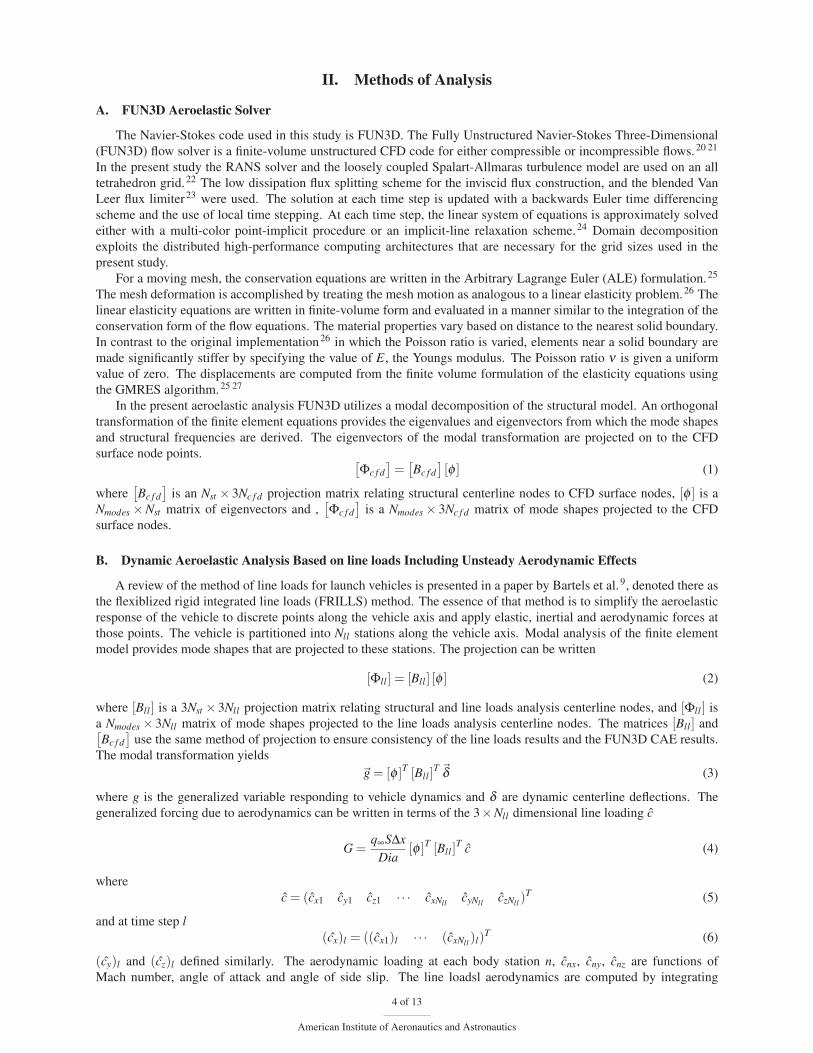
1000 body stations and over 4000 time steps. Figure 3 shows the FFT of the generalized force (mode 1) due to mode 1

excitation at three time step sizes, Δt = 5, 10 and 20. As can be seen in the figure both the real and imaginary responses

at all frequencies are converging as the time step size is reduced. The response at all frequencies using Δt = 10 is nearly

identical to that using Δt = 5. On the other hand all the results are nearly identical at low frequencies. Since an accurate

modeling of the low frequency response is the primary objective in the following analysis, the solution at Δt = 20 was

considered sufficiently accurate.

Figure 3. Time step study of unsteady Gaussian pulse response (mode 1 on mode 1).

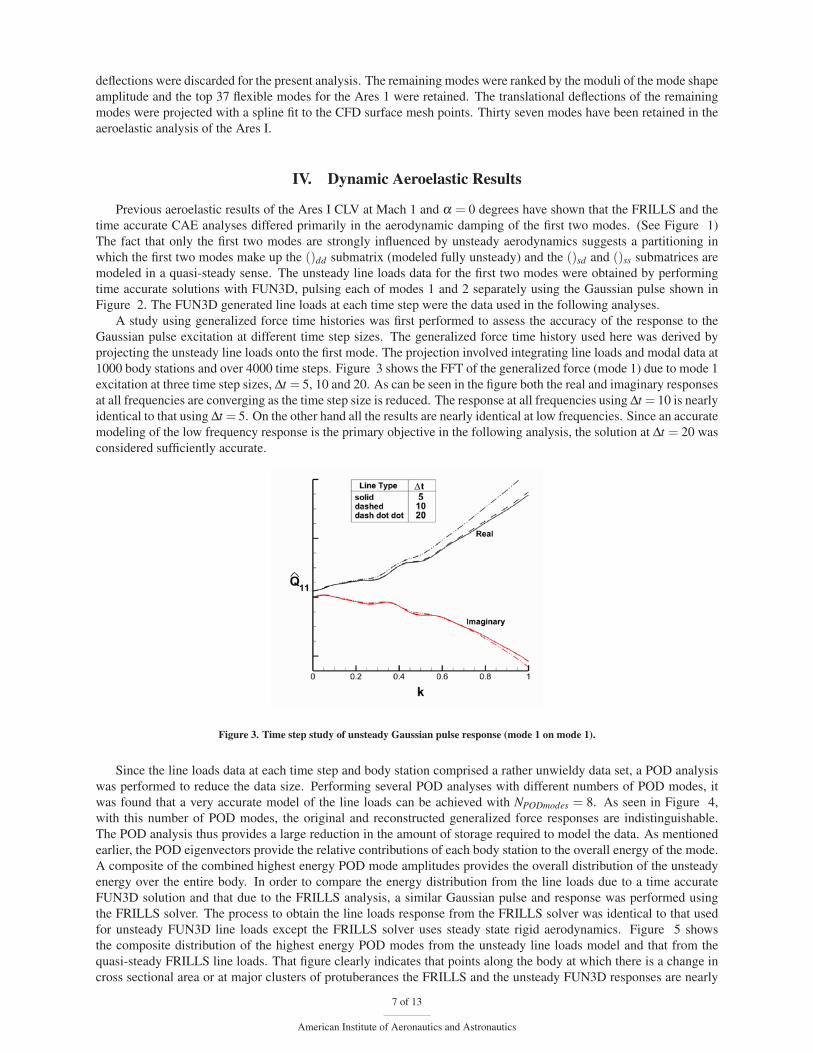
Since the line loads data at each time step and body station comprised a rather unwieldy data set, a POD analysis

was performed to reduce the data size. Performing several POD analyses with different numbers of POD modes, it

was found that a very accurate model of the line loads can be achieved with NPODmodes = 8. As seen in Figure 4,

with this number of POD modes, the original and reconstructed generalized force responses are indistinguishable.

The POD analysis thus provides a large reduction in the amount of storage required to model the data. As mentioned

earlier, the POD eigenvectors provide the relative contributions of each body station to the overall energy of the mode.

A composite of the combined highest energy POD mode amplitudes provides the overall distribution of the unsteady

energy over the entire body. In order to compare the energy distribution from the line loads due to a time accurate

FUN3D solution and that due to the FRILLS analysis, a similar Gaussian pulse and response was performed using

the FRILLS solver. The process to obtain the line loads response from the FRILLS solver was identical to that used

for unsteady FUN3D line loads except the FRILLS solver uses steady state rigid aerodynamics. Figure 5 shows

the composite distribution of the highest energy POD modes from the unsteady line loads model and that from the

quasi-steady FRILLS line loads. That figure clearly indicates that points along the body at which there is a change in

cross sectional area or at major clusters of protuberances the FRILLS and the unsteady FUN3D responses are nearly

7 of 13


identical. These areas are at the LAS nozzles, the CEV module and fairing, the upper stage cluster of protuberances,

the first stage rings and the aft skirt. However, the time accurate modeling of the unsteady line loads also has high

energy content at locations away from cross sectional area changes. These areas include the long unchanging region of

the upper stage and the first stage SRB. This indicates that a fully time accurate solution is required to capture all of the

unsteady energy. It also shows that a quasi-steady model only provides energy content at points of geometry change

while in fact unsteady energy is distributed both at and away from cross sectional area changes. It is also note worthy

that the frustum dynamics due to the time accurate solution is much larger than that due to the FRILLS analysis. Also

shown in that figure are the generalized force responses integrated from the line loads. The difference in the unsteady

and quasi-steady responses is clearly seen in that figure.

Figure 4. Comparison of FUN3D and POD approximation of unsteady mode 1 response (The reconstructed solution is from unsteady lineloads).

(a) line load POD eigenvectors (b) Generalized force 1

Figure 5. Comparison of unsteady FUN3D and FRILLS responses due to 1st mode Gaussian pulse.

8 of 13


Having a POD model of the unsteady line loads due to an excitation of the first two modes, the following steps

were taken to create a state space model of the flexible launch vehicle:

1. Choose the modes (rigid body or higher frequency flexible) to be included in the quasi-steady analysis.

In the present case, flexible modes 3-37 have been selected, although other modes may also be included

such as rigid body modes.

2. The unsteady line loads due to exitation of modes 1 and 2 (reconstructed from the POD model) are

projected at each time step to each of 37 modes. This produces a generalized force time history of all 37

modes due to excitation of the first two modes.

3. An FFT analysis was performed on the generalized force responses integrated from the line loads.

4. A Roger approximation with 20 lag states (NR = 20) using equation 16 is calculated for the first two

modes. This produces the ()dd submatrices.

5. A Roger approximation using equation 17 is calculated for modes 3-37. This produces the ()ds subma-

trices.

6. The ()sd and ()ss submatrices are derived using quasi-steady FRILLS line loads data. The computation

of these submatrices is no different than for a purely quasi-steady FRILLS analysis.

Figure 6 shows the FFT of the generalized force submatrix (Q)dd (comprised of data from modes 1 and 2) and the

Roger approximation of that data as a function of reduced frequency. The Roger approximation uses 20 unsteady

aerodynamic states (i.e. NR = 20). It can be seen in this figure that the Roger approximation with 20 states quite

accurately represents the generalized force data over the entire reduced frequency range. As an additional test, the

time history of the mode 1 generalized force due to the Gaussian pulse excitation was reproduced using the Roger

approximation. In Figure 7, this result is compared with the generalized force time history of mode 1 obtained

directly from the FUN3D modal pulse solution. The Roger model reproduces the original data very accurately up to

0.55 seconds. Although a slight deviation can be seen in the last 0.1 second of the simulation, the overall agreement

is excellent.

Having verified that the POD, the FFT and Roger models all accurately reproduce the data, the model is applied

to the aeroelastic simulation of the Ares I. A state space model was constructed that included the 20 unsteady aerody-

namic lag states. The state space model of equation 11 is modified by the addition of lag states (ξ ),

χ = [A]χ , χ = {g, g,ξ}T (18)

where

[A] =

⎡⎣ 0 I 0

−M−1Ω −M−1Δ M−1q∞d0 e γ

⎤⎦ . (19)

The damping of equations 18 and 19 was extracted by a log-decrement of a time marching solution. Figure 8

shows the damping of the first 14 modes as a function of frequency at nominal dynamic pressure. The FRILLS and

unsteady FUN3D data from Bartels9 are presented for reference. The present model significantly improves the overall

damping in that the first mode undamping is now captured very well. The second mode is much less strongly damped

than in the FRILLS result, although also slightly less damped than the unsteady FUN3D result.

Figure 9 presents the damping of modes 1 and 2 from the Roger 20 lag state model at dynamic pressures qnom and

1.32qnom, all at Mach 1. The unsteady FUN3D results at qnom from reference 9 overlay the present data. A reduced

order analysis of the Ares I with the AIIM1-TOI model at Mach 1 at successive dynamic pressures was previously

performed by Silva.19 Damping values are shown from that reference. Note that the present and FUN3D aeroelastic

damping values are obtained from a log decrement of the time histories while the damping values from reference 19

were obtained by an eigenvalue analysis. Along with the results of Silva, the present state space model accurately

reproduces the continued undamping of mode 1 with successively higher dynamic pressures. The increasing damping

of mode 2 seen in the unsteady aeroelastic solution of reference 9 is observed in the present results. Furthermore, the

presently computed damping values compare much more favorably with the log decrement values from reference 9

than does the damping of reference 19.

V. Conclusions

A method has been presented to enhance the quasi-steady method of line loads by using unsteady line load data

for selected modes. For the Ares I vehicle with the thrust oscillation isolator structural model the first two modes are

poorly modeled by the quasi-steady method of line loads. Furthermore, these modes are the most likely to couple

9 of 13


(a) Generalized force 11 (b) Generalized force 12

(c) Generalized force 21 (d) Generalized force 22

Figure 6. FFT of generalized force (filled symbol - real, open symbol - imag) and 20 state Roger approximation (line) versus frequency.Data reconstructed from unsteady line loads.

10 of 13


Figure 7. Time history of response (The reconstructed solution is derived from unsteady line loads).

Figure 8. Frequency versus damping, qnom. Figure 9. Frequency versus damping, q∞ = qnom,1.32qnom.

11 of 13


with rigid body modes and lead to potential controllability issues. In the present paper a Gaussian pulse is applied

to the first two vehicle bending modes and a time history of the line loads response is acquired. Proper orthogonal

decomposition is used to reduce the volume of line loads data. The Roger approximation is then used to derive a state

space model that can be integrated into the quasi-steady line loads model. The results of this study can be summarized

as follows:

1. The method of dividing the aeroelastic problem into fully unsteady and quasi-steady partitions has

yielded a relatively efficient way of introducing unsteady aerodynamics because a limited number of CFD

pulse/response solutions are required.

2. Proper orthogonal decomposition of the time history of the line loads data has successfully reduced the

data required for an accurate unsteady aerodynamic model.

3. The time history of the unsteady line loads provides additional insight into the flow physics not available

from the integrated generalized forces alone.

One aspect of this method not investigated here is the addition of rigid body modes, or alternate higher frequency

modes in a quasi-steady sense. Addition of these modes in a quasi-steady sense should be easy since doing so involves

retracing steps 2, 3, 5 and 6 of the method outlined above. Adding modes in a quasi-steady sense does not involve

additional unsteady CFD system identification solutions. The pulse shape used here was a Gaussian pulse of each of

the first two modes separately. The use of other pulse functions or the excitation of all modes (in this case modes 1

and 2) simultaneously was not investigated. Finally, the Roger approximation was used to create the state space model

of the unsteady aerodynamics. Future examination of other time domain methods of system identification would be

helpful.

References1Hanson, P. W. and Doggett, R. V., “Aerodynamic Damping and Buffet Response of an Aeroelastic Model of the Saturn I Block II Launch

Vehicle,” NASA Technical Note NASA TN D-2713, 1965.2Doggett, R. V. and Hanson, P. W., “An Aeroelastic Model Approach for the Prediction of Buffet Bending Loads on Launch Vehicles,” NASA

Technical Note NASA TN D-2022, 1963.3Ericsson, L. E. and Pavish, D., “Aeroelastic Vehicle Dynamics of a Proposed Delta II 7920-10L Launch Vehicle,” Journal of Spacecraft and

Rockets, Vol. 37, No. 1, 2000, pp. 28–38.4Ericsson, L. E., “Aeroelastic Instability Caused by Slender Payloads,” Journal of Spacecraft, Vol. 4, No. 1, 1967, pp. 65–73.5Ericsson, L. E., “Unsteady Flow Separation Can Endanger the Structural Integrity of Aerospace Launch Vehicles,” Journal of Spacecraft

and Rockets, Vol. 38, No. 2, 2001, pp. 168–179.6Hanson, P. W. and Doggett, R. V., “Aerodynamic Damping of a 0.02-Scale Saturn SA-1 Model Vibrating in the First Free-Free Bending

Mode,” NASA Technical Note NASA TN D-1956, 1963.7Azevedo, J. L. F., “Aeroelastic Analysis of Hammerhead Payloads,” No. 2307, 1988.8Reding, J. P. and Ericsson, L. E., “Effect of Aeroelastic Considerations on Seasat-A Payload Shroud Design,” Journal of Spacecraft, Vol. 18,

No. 3, 1981, pp. 241–247.9Bartels, R., Chwalowski, P., Massey, S., Heeg, J., Wieseman, C., and Mineck, R., “Computational Aeroelastic Analysis of the Ares Launch

Vehicle During Ascent,” 28th AIAA Applied Aerodynamics Conference, No. 4374, 2010.10Trikha, M., Mahapatra, D. R., Gopalakrishnan, S., and Pandiyan, R., “Analysis of Aeroelastic Stability of a Slender Launch Vehicle using

Aerodynamic Data,” 46th AIAA Aerospace Sciences Meeting, No. 310, 2008.11Azevedo, J. L. F., “Aeroelastic Analysis of Launch Vehicles in Transonic Flight,” Journal of Spacecraft, Vol. 26, No. 1, 1989, pp. 14–23.12Bigarella, E. D. V., Basso, E., and Azevedo, J. L. F., “Multigrid Adaptive-Mesh Turbulent Simulations of Launch Vehicle Flows,” 21st AIAA

Applied Aerodynamics Conference, No. 4076, 2003.13Bigarella, E. D. V. and Azevedo, J. L. F., “Numerical Study of Turbulent Flows over Launch Vehicle Configurations,” Journal of Spacecraft

and Rockets, Vol. 42, No. 2, 2005, pp. 266–276.14Scalabrin, L. C. and Azevedo, J. L. F., “Finite Volume Launch Vehicle Flow Simulations on Unstructured Adaptive Meshes,” 41st AIAA

Aerospace Sciences Meeting and Exhibit, No. 601, 2003.15Azevedo, J. L. F., “Aeroelastic Analysis of Launch Vehicles in Transonic Flight,” 26th AIAA Aeroscience Meeting and Exhibit, No. 708,

1987.16Scalabrin, L. C., Azevedo, J. L. F., Teixeira, P. R. F., and Awruch, A. M., “Three Dimensional Flow Simulations with the Finite Element

Technique over a Multi-Stage Rocket,” 40th AIAA Aerospace Sciences Meeting and Exhibit, No. 408, 2002.17Azevedo, J. L. F., “Aeroelastic Analysis of Hammerhead Payloads,” 29th AIAA Structures, Structural Dynamics and Materials Conference,

No. 2307, 1988.18Capri, F., Mastroddi, F., and Pizzicaroli, A., “Linearized Aeroelastic Analysis for a Launch Vehicle in Transonic Flight,” Journal of Space-

craft and Rockets, Vol. 43, No. 1, 2006, pp. 92–104.19Silva, W., Vatsa, V., and Biedron, R., “Reduced order models for the aeroelastic analysis of the Ares Vehicles,” 28th AIAA Applied Aerody-

namics Conference, No. 4375, 2010.20Anderson, W. K., Rausch, R. D., and Bonhaus, D. L., “An Implicit Upwind Algorithm for Computing Turbulent Flows on Unstructured

Grids,” Computers and Fluids, Vol. 23, No. 1, 1994, pp. 1–22.21NASA LaRC, Hampton, VA, FUN3D Manual, Nov. 2008, http://fun3d.larc.nasa.gov.22Spalart, P. R. and Allmaras, S. R., “One-Equation Turbulence Model for Aerodynamic Flows,” 30th AIAA Aerospace Sciences Meeting and

Exhibit, No. 439, 1992.

12 of 13


23Vatsa, V. N. and White, J. A., “Calibration of a Unified Flux Limiter for Ares-Class Launch Vehicles from Subsonic to Supersonic Speeds,”

56th Propulsion Meeting 5, JANNAF, III, April 2009.24Nielsen, E. J., Lu, J., Park, M. A., and Darmofal, D. L., “An Exact Dual Adjoint Solution Method for Turbulent Flows on Unstructured

Grids,” Computers and Fluids, Vol. 33, No. 9, 2004, pp. 1131–1155.25Biedron, R. T. and Thomas, J. L., “Recent Enhancements To The FUN3D Flow Solver For Moving-Mesh Applications,” 47th AIAA

Aerospace Sciences Meeting, No. 1360, 2009.26Nielsen, E. J. and Anderson, W. K., “Recent Improvements in Aerodynamic Design Optimiation on Unstructured Meshes,” AIAA Journal,

Vol. 40, No. 6, 2002, pp. 1155–1163.27Saad, Y. and Schultz, M. H., “GMRES: A Generalized Minimum Residual Algorithm for Solving Nonsymmetric Linear Systems,” SIAM

Journal of Scientific and Statistical Computing, Vol. 7, 1986, pp. 856–869.28Samareh, J. A., “Discrete Data Transfer Technique for Fluid-Structure Interaction,” 18th AIAA Computational Fluid Dynamics Conference,

No. 4309, 2007.29Marques, A. N. and Azevedo, J. L. F., “Application of CFD-Based Unsteady Forces for Efficient Aeroelastic Stability Analyses,” 44th AIAA

Aerospace Sciences Meeting, No. 250, 2006.30Pirzadeh, S. Z., “Advanced Unstructured Grid Generation for Complex Aerodynamic Applications,” 26th AIAA Applied Aerodynamics

Conference, No. 7178, 2008.31Bartels, R., Vatsa, V., Carlson, J.-R., Park, M., and Mineck, R., “FUN3D Grid Refinement and Adaptation Studies for the Ares Launch

Vehicle,” 28th AIAA Applied Aerodynamics Conference, No. 4372, 2010.

13 of 13


a quasi-steady flexible launch vehicle stability analysis ... · pdf filea quasi-steady...

Documents