a rating-based sovereign credit risk model: theory and ... annual meetings/2014-… · a...
TRANSCRIPT

A Rating-Based Sovereign Credit Risk Model: Theory andEvidence∗
Haitao Li†, Tao Li‡, and Xuewei Yang§
January 6, 2014
Abstract
We develop a rating-based continuous-time model of sovereign credit risk with closed-form solu-tions for a wide range of credit derivatives. In our model, rating transition follows a continuous-time Markov chain, and countries with same credit rating share similar level of default risk. A par-simonious version of our model, with only 16 parameters, one common and one country-specificfactor, can simultaneously capture the term structure of CDS spreads of 34 in-sample and 34 out-of-sample countries well. On average, the common factor explains more than 60% of the variationsof the CDS spreads of both the in-sample and out-of-sample countries, and 80% of the variations ofthe common factor is explained by the CBOE VIX index, the 5-year US Treasury rate, and the CDXNA IG Index.
Keywords: Credit Rating, Sovereign Credit Risk, Credit Default Swap, Systematic RiskJEL Classification: G22, G33
∗We thank Stephen Figlewski, Masaaki Kijima, and seminar participants at Kyoto University, Nanjing University, Shang-hai Finance University, the University of Tokyo, the PKU-Tsinghua-Stanford Joint Conference in Quantitative Finance, andthe 2014 Econometric Society Winter Meeting for helpful comments and suggestions. We are responsible for any remainingerrors.
†Cheung Kong Graduate School of Business, Beijing 100738, China, email: [email protected].‡Department of Economics and Finance, City University of Hong Kong, Kowloon, Hong Kong, email: [email protected].§School of Management and Engineering, Nanjing University, Nanjing 210093, China, email: [email protected].

A Rating-Based Sovereign Credit Risk Model: Theory and Evidence
Abstract
We develop a rating-based continuous-time model of sovereign credit risk with closed-form solu-
tions for a wide range of credit derivatives. In our model, rating transition follows a continuous-
time Markov chain, and countries with the same credit rating share a similar level of default risk.
A parsimonious version of our model, with only 16 parameters, as well as one common and one
country-specific factor, can simultaneously capture the term structure of CDS spreads of 34 in-
sample and 34 out-of-sample countries well. On average, the common factor explains more than
60% of the variations of the CDS spreads of both the in-sample and out-of-sample countries, and
80% of the variations of the common factor is explained by the CBOE VIX index, the 5-year US Trea-
sury rate, and the CDX NA IG Index.
Keywords: Credit Rating, Sovereign Credit Risk, Credit Default Swap, Systematic Risk
JEL Classification: G22, G33

“... we live again in a two-superpower world. There is the US and there is Moody’s. The
US can destroy a country by leveling it with bombs; Moody’s can destroy a country by
downgrading its bonds.”
——Thomas L. Friedman, The New York Times, Feb 22, 1995
1 Introduction
The Eurozone debt crisis has highlighted the importance of sovereign credit risk in global financial
markets. It has also brought back memories of the huge losses that investors in sovereign debts have
suffered in many similar crises in the past two centuries, such as the “Baring Crisis” of the 1890s,
the Latin American debt crisis of the 1980s, and the Mexican and Russian debt crisis of the 1990s. A
large literature has been developed in economics and finance to understand the nature, causes, and
consequences of sovereign debt crisis as well as the pricing and management of sovereign credit risk.
Extensive research over the past decades has revealed important patterns in both the cross-sectional
and time series variations of sovereign credit spreads.
One line of research has focused on the role of credit rating in sovereign credit markets.1 By group-
ing borrowers into broad categories with similar credit qualities, credit rating provides a first-order
approximation of the level of default risk. Numerous studies, such as Cantor and Packer (1996) , have
shown that sovereign credit rating reflects the macroeconomic fundamentals of a country and that
there are significant variations in sovereign credit spreads across different rating classes. Moreover,
rating transition represents a discrete and material change in the credit quality of a borrower. During
the recent global financial crisis, downgrades of sovereign governments (from the PIIGS countries in
Europe to the strongest borrower in the world, the US government) by credit rating agencies have re-
sulted in violent reactions in the sovereign CDS market. Several recent event studies have empirically
documented the significant impacts of rating changes on sovereign CDS spreads for both developed
and emerging market countries.2 However, this strand of literature does not explicitly model the dy-
1There is a huge literature on the impact of credit rating agencies for both corporate and sovereign credit markets. Forbrevity, we refer readers to Kiff et al. (2012) for a partial review of the literature on sovereign credit rating.
2For example, based on rating changes and CDS spreads of 22 emerging market countries between 2001 and 2008,Ismailescu and Kazemi (2010) document the direct effects of announcements of sovereign rating changes on CDS spreadsof the event countries and the spillover effects on other emerging market countries. Afonso et al. (2012) show that for a large
1

namic evolution of sovereign credit risk.
Another line of research, based on the reduced-form approach of Duffie and Singleton (1999 and
2003), has shown that time series fluctuations of sovereign credit spreads are mostly driven by com-
mon risk factors. For example, Pan and Singleton (2008) show that one common principal component
(PC) explains more than 90% of the variations of the CDS spreads of three geographically dispersed
countries: Mexico, Turkey, and Korea. Longstaff et al. (2011) conclude that the CDS spreads of 26
developed and emerging market countries are driven primarily by the VIX index, US equity, and high-
yield factors. Based on a sovereign credit risk model with a common and a country-specific factor,
Ang and Longstaff (2013) show that the US and European systemic factors extracted from the CDS
spreads of the US government, 10 individual US states, and 11 EMU sovereigns are highly correlated
with one another and are strongly related to financial market variables.
In this paper, inspired by the two lines of research, we develop a rating-based continuous-time
model for sovereign credit risk that explicitly incorporates the well-known cross-sectional and time
series properties of sovereign credit spreads and provides closed-form solutions for a wide range of
credit derivatives.3 In our model, the credit rating of each country follows a continuous-time Markov
chain characterized by a common transition matrix, and countries within a given rating category share
similar default intensity. Following Ang and Longstaff (2013), we assume that the default risk of a
sovereign borrower is driven by a common and a country-specific factor. The common factor drives the
rating transition matrix as well as the systematic component of default risk, and the default intensities
of countries in different rating categories have different loadings on the common factor. The country-
specific factor captures the idiosyncratic component of the default risk of each individual country.4
The number of parameters of our model does not increase with the number of countries, given that
group of European countries, the reactions of CDS spreads to negative rating events have increased since the Lehman Broth-ers bankruptcy on September 15, 2008. They also report spillover effects of rating announcements, particularly from lowerrated countries to higher rated ones.
3While a series of studies, such as Jarrow et al. (1997), Lando (1998), Kijima (1998), Das and Hanouna (1996),Arvanitis et al. (1999), Huge and Lando (1999), and Li (2000), have considered credit rating for the pricing of corporate de-fault risk, our model is one of the first rating-based models in the literature on sovereign credit risk.
4Ang and Longstaff (2013) use Germany as the systemic factor for European countries and US for individual states. Thismodeling choice is perfectly sensible given the purpose of their research. Given that we want to price CDS spreads ofcountries from different parts of the world, such as Europe, North and Latin America, Asia, and Middle East, we allow eachcountry to have its own country-specific factor in our model.
2

countries share the same set of parameters for the country-specific factor.
One of the most appealing features of our rating-based approach is that by explicitly modeling the
cross-sectional and time series properties of sovereign credit spreads, it can simultaneously capture the
credit spreads of multiple countries under a parsimonious and unified modeling framework. Given the
strong dependence of sovereign credit spreads on credit rating, incorporating rating information into
the existing reduced-form models significantly enhance these models’ capability to capture the cross-
sectional variations of sovereign credit spreads. Therefore, while the existing reduced-form models
mostly focus on pricing the credit risk of individual countries, the ultimate goal of our rating-based
model is to capture the credit spreads of all countries, which makes it possible to analyze the default
risk of portfolios of sovereign credit instruments.
Another important advantage of our rating-based model is that it naturally captures both contin-
uous evolution and discrete change in the default risk of a sovereign borrower due to rating transi-
tion. Existing reduced-form models, which assume that the default intensity of a sovereign borrower
follows a continuous diffusion process, would have difficulty in capturing the dramatic increases in
the default risk of sovereign borrowers due to rating downgrades. Historically, a highly rated bor-
rower rarely defaults immediately. Instead, it is more likely to be downgraded first before defaults.
Therefore, the credit risk of a sovereign borrower consists of the risk of default as well as the risk of
downgrading. Moreover, rating downgrades (particularly from investment grade to non-investment
grade) could seriously affect the market’s perception of the credit quality of a borrower and thus limit
its access to capital markets. Therefore, incorporating rating information into existing reduced-form
sovereign credit risk models could help to capture the default risk of sovereign borrowers more com-
pletely and yield better insights about the sovereign credit market.5
By incorporating fundamental information (summarized in credit ratings) into existing reduced-
form models, our model avoids overfitting the data and improves the efficiency of model estimation.
While existing reduced-form models choose latent default factors to match the observed credit spreads
5Our paper is most closely related to Farnsworth and Li (2007) and Remolona et al. (2008). While Farnsworth and Li(2007) develop a rating-based model for corporate credit risk, our paper is one of the first that studies the effect of rating onthe pricing of sovereign CDS spreads in a dynamic setting.
3

of individual countries, our approach requires countries with similar credit ratings to share similar
level of default risk. As a result, pricing errors under our model reflect inconsistencies between ob-
served credit spreads and underlying credit rating and therefore could be strong signs of future rating
changes. Since countries with the same credit rating share similar level of default risk, our approach
uses the credit spreads of all countries jointly to estimate the model and significantly increase the es-
timation efficiency of the common default factor. This case is similar to the portfolio approach in the
equity literature, which estimates asset pricing models using portfolios of securities with similar risk
exposures instead of individual securities.
Consistent with our objective, we apply our parsimonious model with only 16 parameters, one
common and one country-specific factor, to capture the term structure of CDS spreads of 68 countries
between January 2004 and March 2012. The ratings of these countries are obtained from Standard
& Poor’s and are grouped into 7 broad rating categories: AAA, AA, A, BBB, BB, B, and CCC. While
existing models for sovereign credit risk are typically estimated country by country, we estimate our
rating-based model simultaneously using the term structure of CDS spreads of the 34 in-sample coun-
tries, which have the most observations via maximum likelihood. We then use the estimated model to
price the CDS spreads of the 34 out-of-sample countries, which have fewer observations. We choose
the common factor to match the average CDS spreads of the in-sample countries across all maturities
and use it to price the out-of-sample countries. We choose the country-specific factor to match the av-
erage CDS spreads of each in-sample and out-of-sample country over all maturities given the common
factor.
Overall, our rating-based model can capture the term structure of CDS spreads of the 34 in-sample
countries reasonably well. The model has small average absolute pricing errors relative to the average
bid-ask spreads of the CDS spreads, particularly for intermediate maturities and ratings. Notably, our
extremely parsimonious model has equally good or even better pricing performance for the 34 out-of-
sample countries. For a wide range of out-of-sample countries, the average absolute pricing errors at
intermediate maturities (2 to 7 years) are lower or at par with the average bid-ask spreads.
Although we find relatively large pricing errors for certain countries during certain parts of our
4

sample period, in almost all cases, the pricing errors reflect inaccuracies in the credit ratings of these
countries. For example, in 2004 and 2005, our model has large pricing errors for some Latin American
countries, such as Brazil and Colombia. News reports during this time suggest that market partici-
pants believe that these countries are underrated and their ratings do not fully reflect the improved
macroeconomic fundamentals due to rising exports, declining deficits, and strengthening local curren-
cies. The large pricing errors disappear as the countries are gradually upgraded. We also find relatively
large pricing errors for some of the Eurozone countries during the 2008 global financial crisis and the
2011 European debt crisis. The unstable ratings of these countries, as evidenced by their subsequent
credit downgrades and negative watches, significantly affect their CDS spreads.
Given the important role played by the common factor for sovereign CDS pricing, we examine the
nature of the common factor from several different perspectives. We first show that our model with
the common factor alone, i.e., setting all country-specific factors to be zero, can explain more than 60%
of the variations of the CDS spreads of the 34 in-sample and 34 out-of-sample countries on average.
Therefore, by simply adding a cross-sectional dimension to existing reduced-form models with only
the common factor, we obtain an extremely parsimonious model that can capture the majority of the
variations of the CDS spreads of most countries. Since we do not have a country-specific factor, the 34
out-of-sample countries are purely out of sample. As a result, we expect the model to work equally
well for additional out-of-sample countries.
Following existing studies, we then explore the economic forces that drive the common factor, the
market price of default risk, and the credit risk premium. The common factor extracted from our model
can explain a large fraction of the CDS spreads of most countries and has close connections to financial
market variables. For example, we find that the VIX index, the 5-year constant maturity Treasury rates,
and the CDX NA IG can explain more than 80% of the variations of the common factor, the market price
of risk, and the credit risk premium. We also find that the credit risk premium increases dramatically
during the global financial crisis and the European debt crisis. This is especially more pronounced for
CDS with higher ratings and longer maturities.
The rest of the paper is organized as follows. In Section 2, we develop a general rating-based
5

continuous-time model for sovereign credit risk. We discuss the data used in our empirical study and
the estimation method in Section 3 and report the empirical results in Section 4. Section 5 concludes
the paper.
2 A Rating-Based Sovereign Credit Risk Model
In this section, we first introduce a general rating-based continuous-time model for sovereign credit
risk. We then consider a special version of the model with one common and one country-specific
factor with closed-form solutions for a wide range credit derivatives. Finally, we consider a multi-
factor extension of the baseline model. Throughout the analysis, we assume there exists a risk-neutral
probability space (Ω,F , F,Q), under which all securities can be priced appropriately. All expectations
are taken under this risk-neutral probability measure Q.
2.1 A General Model with Credit Ratings
Suppose all sovereign borrowers can be classified into K possible credit rating categories and the rating
for each country follows a continuous-time Markov chain characterized by a common transition matrix
Q(t) = qij(t)i, j=1,...,K,
where ∑Kj=1 qij = 0. Intuitively, over a short horizon ∆t, the probability for a rating change from i to
j 6= i is qij∆t.
Following Farnsworth and Li (2007) or Li (2000), we also assume that countries in the same rating
category share the same default intensity. That is, if a country is rated
CR(t) ∈ 1, · · · , K,
then its hazard rate of default is hCR(t−)(t). Let H be a diagonal matrix with its diagonal element
Hii = hi(t), which represents the default intensity of a country with a rating i. Let P(t, T) be the price
6

vector associated with a payoff P(T) at maturity T, our goal is to derive a pricing equation for P (t, T) .6
Let CR(t−) = i and applying Ito’s Lemma to PCR(t)(t, T) yields
Et
[dPCR(t)(t, T)
]= Et [dPi(t, T)] +
K
∑k=1
qik (Pk(t, T) − Pi(t, T)) dt + hi(t)(
PDi (t) − Pi(t, T)
)dt,
where PDi is the payoff at default. As no-arbitrage requires Et
[dPCR(t)(t, T)
]= r(t)PCR(t−)(t, T) dt, we
have
Et[dPi(t, T)] +K
∑k=1
qik (Pk(t, T) − Pi(t, T)) dt + hi(t)(
PDi (t) − Pi(t, T)
)dt = r(t)Pi(t, T) dt,
where r is the risk-free interest rate. By the fact that ∑Kk=1 qik = 0, we can rewrite the equation in terms
of vectors and matrices as
Et[dP(t, T)] = [r(t)I + H(t)]P(t, T) dt − Q(t)P(t, T) dt − H(t)PD(t) dt, (1)
where Q, H, and PD are some suitable measurable stochastic processes.
It can be shown that pricing equation (1) is equivalent to
P(t, T) = Et
[exp
(−∫ T
tr(s) ds
)Φ(t, T)P(T)
+∫ T
texp
(−∫ s
tr(a)da
)Φ(t, s)H(s)PD(s) ds
], (2)
where Φ(t, s) is defined as the solution to the following ordinary differential equation
dΦ(t, s)dt
= −[Q(t) − H(t)]Φ(t, s) (3)
with boundary condition Φ(s, s) = I.
Pricing equation (2) has a natural and intuitive interpretation. Φ(t, s) is the probability matrix that
6For a coupon bond, P(T) = 1. The model can easily price credit linked notes by setting appropriate rating-dependentterminal payoff P(T).
7
the security has not defaulted up to time s, H(s)ds is the default probability matrix over ds, PD(s) is
the cash flow vector when the security defaults, and P(T) is the cash flow vector if the security does
not default up to T. Thus, the summation (integration) over all of the expected discounted cash flows
under the risk-neutral probability yields the price of the security.
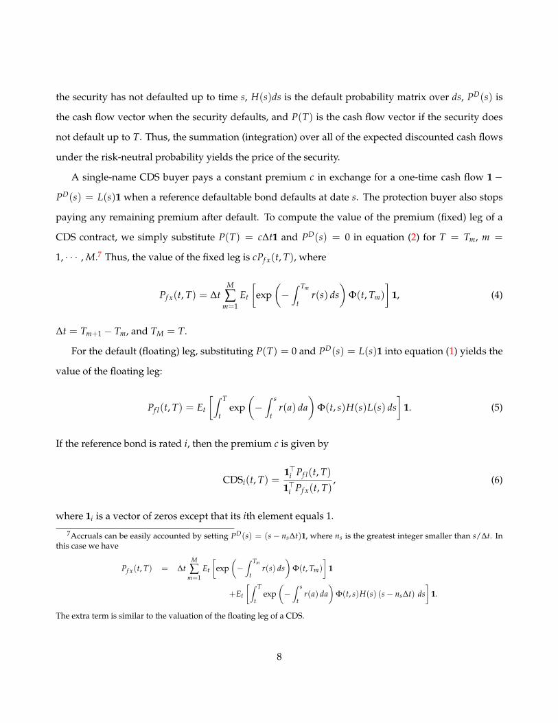
A single-name CDS buyer pays a constant premium c in exchange for a one-time cash flow 1 −
PD(s) = L(s)1 when a reference defaultable bond defaults at date s. The protection buyer also stops
paying any remaining premium after default. To compute the value of the premium (fixed) leg of a
CDS contract, we simply substitute P(T) = c∆t1 and PD(s) = 0 in equation (2) for T = Tm, m =
1, · · · , M.7 Thus, the value of the fixed leg is cPf x(t, T), where
Pf x(t, T) = ∆tM
∑m=1
Et
[exp
(−∫ Tm
tr(s) ds
)Φ(t, Tm)
]1, (4)
∆t = Tm+1 − Tm, and TM = T.
For the default (floating) leg, substituting P(T) = 0 and PD(s) = L(s)1 into equation (1) yields the
value of the floating leg:
Pf l(t, T) = Et
[∫ T
texp
(−∫ s
tr(a) da
)Φ(t, s)H(s)L(s) ds
]1. (5)
If the reference bond is rated i, then the premium c is given by
CDSi(t, T) =1>i Pf l(t, T)1>i Pf x(t, T)
, (6)
where 1i is a vector of zeros except that its ith element equals 1.
7Accruals can be easily accounted by setting PD(s) = (s − ns∆t)1, where ns is the greatest integer smaller than s/∆t. Inthis case we have
Pf x(t, T) = ∆tM
∑m=1
Et
[exp
(−∫ Tm
tr(s) ds
)Φ(t, Tm)
]1
+Et
[∫ T
texp
(−∫ s
tr(a) da
)Φ(t, s)H(s) (s − ns∆t) ds
]1.
The extra term is similar to the valuation of the floating leg of a CDS.
8
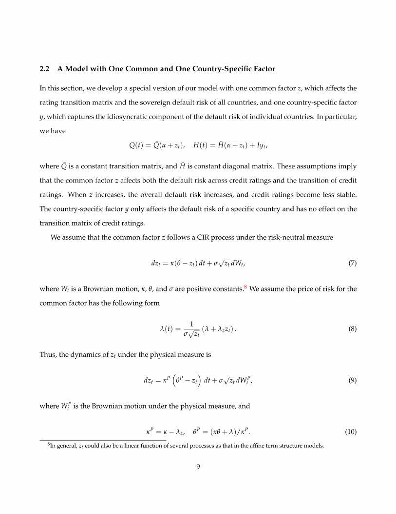
2.2 A Model with One Common and One Country-Specific Factor
In this section, we develop a special version of our model with one common factor z, which affects the
rating transition matrix and the sovereign default risk of all countries, and one country-specific factor
y, which captures the idiosyncratic component of the default risk of individual countries. In particular,
we have
Q(t) = Q(α + zt), H(t) = H(α + zt) + Iyt,
where Q is a constant transition matrix, and H is constant diagonal matrix. These assumptions imply
that the common factor z affects both the default risk across credit ratings and the transition of credit
ratings. When z increases, the overall default risk increases, and credit ratings become less stable.
The country-specific factor y only affects the default risk of a specific country and has no effect on the
transition matrix of credit ratings.
We assume that the common factor z follows a CIR process under the risk-neutral measure
dzt = κ(θ − zt) dt + σ√
zt dWt, (7)
where Wt is a Brownian motion, κ, θ, and σ are positive constants.8 We assume the price of risk for the
common factor has the following form
λ(t) =1
σ√
zt(λ + λzzt) . (8)
Thus, the dynamics of zt under the physical measure is
dzt = κP(
θP − zt
)dt + σ
√zt dWP
t , (9)
where WPt is the Brownian motion under the physical measure, and
κP = κ − λz, θP = (κθ + λ)/κP. (10)
8In general, zt could also be a linear function of several processes as that in the affine term structure models.
9

Given this physical dynamics, it is straightforward to derive the transition probability and the likeli-
hood of the systematic factor.
The country-specific factor y, which carries no risk premium, follows a Vasicek process
dyt = κy[θy − yt]dt + σydWyt ,
where Wy is independent of W.
There are different ways to model the loss at default process L. Although we could allow each
country to have its own loss at default or countries in the same rating category to share the same level
of loss of default, for convenience, we assume that all countries share the same level of loss of default.
We also assume that the risk-free interest rate r is independent of z.9 This independence assumption
enables us to separate the expectations between the risk-free rate and default risk components, thus
simplifying the computation of CDS spreads.
2.2.1 Common Factor
The key to compute the pricing formulae (4) and (5) is to compute the following expectations:
Et[Φ(t, T)] and Et[Φ(t, T)H(t)].
Given the affine structure of our model, Φ has a closed-form solution as follows:
Φ(t, T) = Ω exp(
Λ∫ T
t(α + za)da
)Ω−1,
where ΩΛΩ−1 = Q − H, and Λ is a diagonal matrix with its elements as eigenvalues of Q − H. Since
Λ is a diagonal matrix, we have that
exp(
Λ∫ s
t(α + za) da
)9This independence assumption can be relaxed through a linear relation between r and z, such as r(s) = X(s) + ρzt, where
X and z are independent, and X represents other factors that affect the default-free term structure.
10

is also a diagonal matrix with its diagonal element i
exp(
Λii
∫ s
t(α + za) da
).
It is straightforward to show that
Et[Φ(t, s)] = Ω Γ1(τ, zt)Ω−1, (11)
where τ = s − t, and Γ1 is a diagonal matrix with its diagonal elements equal to
Γ1ii(τ, zt) = p0(τ, αΛii)p1(τ, zt, Λii).
We can also show that
Et[Φ(t, s)H(s)] = Ω Γ2(τ, zt)Ω−1H, (12)
where Γ2 is a diagonal matrix with its diagonal elements equal to
Γ2ii(τ, zt) = p0(τ, αΛii)[αp1(τ, zt, Λii) + p2(τ, zt, Λii)],
p0(τ, β) = exp(βτ),
p1(τ, zt, β) = Et
[exp
(β∫ s
tza da
)]= A(β, τ)eB(β,τ)zt , (13)
p2(τ, zt, β) = Et
[zs exp
(β∫ s
tza da
)]= [C(β, τ) + D(β, τ)zt]eB(β,τ)zt ,
for any β, and
A(β, τ) = exp(
κθ(φ + κ)σ2 τ
)(1 − γ
1 − γeφτ
) 2κθσ2
,
B(β, τ) =κ − φ
σ2 +2φ
σ2(1 − γeφτ),
11

C(β, τ) =κθ
φ(eφτ − 1) exp
(κθ(φ + κ)
σ2 τ
)(1 − γ
1 − γeφτ
) 2κθσ2 +1
,
D(β, τ) = exp(
κθ(φ + κ) + φσ2
σ2 τ
)(1 − γ
1 − γeφτ
) 2κθσ2 +2
,
φ =√−2βσ2 + κ2, γ =
κ + φ
κ − φ.
Thus, it is straightforward to obtain the value of the fixed leg via equation (4). A numerical inte-
gration is needed to compute (5) for the floating leg as follows:
Pf l(t, T) = Ω[∫ T
tP0(t, s) Γ2(s − t, zt) ds
]Ω−1HL1,
where P0(t, s) is the price of default-free zero coupon bonds.
2.2.2 Country-Specific Factor
With the addition of the country-specific factor y, equations (11) and (12) become
Et[Φ(t, s)] = p1(τ, yt)Ω Γ1(τ, zt)Ω−1 (14)
and
Et[Φ(t, s)H(s)] = Ω [ p1(τ, yt)Γ2(τ, zt) + p2(τ, yt)Γ1(τ, zt)]Ω−1H, (15)
where Γ1 and Γ2 are the same as defined previously, and pk-s are given by (see, e.g., Jamshidian, 1989)
p1(τ, yt) = Et
[exp
(−∫ s
tyada
)]= A(τ)e−B(τ)yt ,
p2(τ, yt) = Et
[ys exp
(−∫ s
tyada
)]=[C(τ) + D(τ)yt
]e−Bτyt ,
where τ = s − t, and
A(τ) = exp
((θy −
σ2y
2κ2y
)(B(τ) − τ) −
σ2y B2(τ)
4κy
),
12

B(τ) =1 − e−κyτ
κy, C(τ) =
(κyθyB(τ) −
σ2y B2(τ)
2
)A(τ), D(τ) = e−κyτ A(τ).
Substituting these formulae in conjunction with the default-free term structure
P0(t, s) = Et
[exp
(−∫ s
trada
)]
in equations (4), (5), and (6) yields the CDS spreads.
2.3 A Multi-Factor Extension
The model with one common and one country-specific factor can be easily extended to have multiple
common and country-specific factors. The common factors can be modeled as follows:
Q(t) = Q[α0 + α>zt], H(t) = H[α0 + α>zt],
where Q is a constant transition matrix, H is a constant diagonal matrix, and z is an k × 1 vector with
kth element zk satisfies
dzkt = κk[θk − zk
t ]dt + σk
√zk
t dWkt ,
where Wkt is independent across k. In this case, we only need to redefine Γ as
Γ1ii(τ, zt) = p0(τ, α0Λii) ∏
k=1p1(τ, zk
t , αkΛii)
and
Γ2ii(τ, zt) = p0(τ, α0Λii) ∑
n=0αn p2(τ, zn
t , αnΛii) ∏k 6=n
p1(τ, zkt , αkΛii),
where ps are similar to those given by (13), except that p2(·, z0, ·) = 1. Adding one or more country-
specific factor(s) into this model is evidently straightforward.
13

3 Data and Estimation Method
In this section, we first introduce the data used in our empirical analysis, which include the term
structure of CDS spreads, the corresponding bid-ask spreads as well as the credit ratings of the 68
countries. We then discuss the estimation of our rating-based sovereign credit risk model with one
common and one country-specific factor using maximum likelihood.
3.1 Data
We obtain the sovereign CDS spreads from Credit Market Analysis Ltd (CMA), which collects OTC
market data on credit derivatives. The sample consists of monthly quotes of CDS spreads with matu-
rities of 1, 2, 3, 5, 7, and 10 years from January 2004 to March 2012. In our analysis, we consider 68
countries10 from North America, Europe, Asia/Pacific, Middle East, Latin America, and Africa. The
discount bond prices P0(t, u) in the valuation formula are bootstrapped from the US Dollar LIBOR and
swap rates downloaded from Bloomberg.
Table 1 provides important summary information of the 68 countries, which includes credit rating,
average 5-year CDS spread, average bid-ask spread of 5-year CDS spread, number of observations, and
number of rating changes for each country. The maximum number of observations for each country
is 99 months. We use the top 34 countries with the most complete observations of the term structure
of CDS spreads to estimate our model in sample. We then use the estimated model to price the CDS
spreads of the other 34 countries with fewer observations out of sample. All the CDS spreads are
denoted in basis points and quoted in US dollars. We use the Standard & Poor’s credit ratings obtained
from Bloomberg. Following previous literature, we ignore minor adjustments such as “+” or “-” to
baseline ratings and obtain seven broad rating categories from AAA to CCC (C and CC are merged into
CCC). Ratings reported in Table 1 represent the rating of each country at the end of the sample period.11
While the ratings of 25 countries (12 in-sample and 13 out-of-sample) remain constant throughout the
sample, certain countries experience up to 5 rating changes during the sample period. The average
10The original dataset covers CDS for 69 countries. We exclude Malta from our analysis, because it has observations foronly six months.
11In the empirical section, we report the complete history of the evolution of the ratings of each country.
14

5-year CDS spreads generally increase when rating deteriorates. The most common ratings are A and
BBB, whereas the least common one is CCC, which belongs to Greece.12 Panel A of Table 2 reports the
frequency of rating changes of the 34 countries used for in-sample model estimation. In total, the 34
countries have experienced 40 rating changes (under our reclassification of ratings) during the sample
period. Interestingly, rating transitions typically occur between two adjacent ratings. For example,
there are 4 rating changes from A to AA. This empirical fact motivates our parametrization of the
rating transition matrix as a tri-diagonal matrix in Section 3.2. The top-left panel of Figure 1 plots the
numbers of quarterly rating changes and the average 5-year CDS spreads of the 34 in-sample countries.
The top-right panel of Figure 1 also reports the numbers of rating downgrades during the sample
period. Notably, rating changes and downgrades tend to increase when the CDS spreads widen.
Panel B of Table 2 reports the average CDS spreads for countries in different rating categories and at
different maturities. Panel C of Table 2 also reports the average bid-ask spreads at different maturities
and credit ratings. On average, we find an upward sloping term structure of CDS spreads for ratings
above BB. For the CCC rating, the term structure of CDS spread is downward sloping. The CDS
spreads increase monotonically when ratings worsen. The bottom two panels of Figure 1 provide time
series plots of the average 5-year CDS spreads at different ratings. We see a monotonically negative
relation between rating and average CDS spreads. We also see huge spikes in the CDS spreads during
the global financial crisis and European debt crisis.
3.2 Maximum Likelihood Estimation
We use the model with one common and one country-specific factor (with α = 0) presented in Section
2.2 in our empirical analysis. We assume that the loss rate is 60% for all countries regardless their
ratings. To reduce the parameter space, although we allow each country to have its own local factor
yjt, all countries share the same set of parameters for yj. While the yj factor is supposed to capture the
idiosyncratic component of a country’s default risk, it might also capture small deviations from the
12After Greece’s downgrade by the S&P to Selective Default (SD) on February 27, 2012, the CDS spreads of Greece becomeextremely high. For example, the Greece 1-year CDS spreads were 57,166 and 57,644 basis points on February 29, 2012 andMarch 30, 2012, respectively. Thus, we remove the last two month CDS spreads of Greece in our in-sample estimation andall subsequent analyses.
15

average default risk for a particular sovereign credit rating due to our coarse re-classification of the
observed credit ratings.
The parameters are estimated using maximum likelihood. We assume that, on each day, the sum
of the CDS spreads of all countries and all maturities implied by the model with only the common
factor is equal to the sum of the market CDS spreads, such that the pricing function can be inverted
to obtain the common factor z. On each corresponding day and for each country, we assume that the
sum of CDS spreads at all maturities implied by the model with both the common and country-specific
factor equals that of the market quotes, such that we can back out the country specific factor yj given z.
For the j-th country, the contract with maturity M is assumed to be priced with normally distributed
pricing errors with mean zero and standard error σjM.
To estimate the model, we need to compute the log-likelihood of the observed data and the model
implied z and yj. Let εjt be the vector of pricing errors across maturites for the CDS contracts for
country j at time t, and CRj(t) the ratings for country j at time t, then the likelihood function includes
the following four components:
• The likelihood of the pricing error εjt at time t given zt, yjt, and CRj(t), which is Gaussian by
assumption, across countries;
• The likelihood of rating CRj(t) at time t given CRj(t − ∆), zt−∆, and zt across countries;
• The likelihood of yjt given yj(t−∆), which is Gaussian (see, e.g., Jamshidian, 1989), across coun-
tries;
• The likelihood of zt given zt−∆, which is non-central χ2 (see, e.g., Cox et al., 1985).
Similar to that in Farnsworth and Li (2007), we assume that the transition matrix of ratings is 7-
by-7 tri-diagonal, such that the diagonal elements are determined by Qi,i = −Qi,i−1 − Qi,i+1, where
Qi,i−1 = Q21 for the lower diagonal, and Qi,i+1 = Q12 for the upper diagonal. This assumption reduces
the parameter space significantly and is consistent with the frequency of rating transitions reported in
16

Table 2. The transition probabilities of ratings between t − ∆ and t are given by
exp(∫ t
t−∆Qza da
).
However, since we do not have a continuous observation of za, we use the following to approximate
the transition probabilities
EP[
exp(∫ t
t−∆Qza da
)∣∣∣∣ zt−∆, zt
],
where the expectation is under the physical measure.13 H is a 7-by-7 diagonal matrix. To avoid poten-
tial identification problems between Hii-s and the common factor z, we fix the value of H33 at 1.
4 Empirical Results
In this section, we discuss the empirical results of our rating-based model for sovereign CDS pricing.
We first examine the estimated parameters of the model. Then, we show that our parsimonious model
with 16 parameters, one common and one country-specific factor, can price the CDS spreads of the
34 in-sample and 34 out-of-sample countries reasonably well. We also show that the relatively large
pricing errors for certain countries reflect staleness of their credit ratings. Finally, we show that the
common factor on average can explain more than 60% of the variations of the CDS spreads of both the
in-sample and out-of-sample countries and that more than 80% of the variations of the common factor
backed out from our model can be explained by the VIX index, the 5-year US Treasury rate, and the
CDX NA IG index.
4.1 Parameter Estimates
Table 3 reports the maximum likelihood estimates of the parameters of three different versions of our
rating-based model. Model I is the full model as described previously. All the parameter estimates
of Model I are highly significant. To examine the incremental contribution of rating transition, we
13The details of the approximation can be found in the Appendix of Farnsworth and Li (2007).
17

consider Model II, which maintains rating-dependent default intensity but does not allow transitions
between different ratings. Finally, we consider Model III, which does not allow any distinctions be-
tween ratings. Likelihood ratio tests highlight the importance of credit rating in model performance
and overwhelmingly reject Model III against Model II and Model II against Model I. All subsequent
analyses and discussions are solely based on the estimation results of Model I reported in Table 3.
We first highlight the cross-sectional differences in default risk for different rating categories. The
loading of each rating group on the common factor Hii monotonically increases from 0.26 for AAA
rating to 64.32 for CCC rating. These estimates are consistent with the idea that rating captures the
relative ranking of default risk of borrowers and shows that rating is an important factor of capturing
the cross-sectional variations of CDS spreads.
The highly significant parameter estimates of the transition matrix Q highlight the importance of
rating changes. In Table 4, we translate these estimated parameters into the transition probabilities of
rating changes over one year horizon. We find that ratings tend to be very stable and persistent. Under
normal market conditions, a country has more than 90% probability to remain in its current rating
over a one-year horizon. Rating transitions become more likely when the general level of default risk
measured by the common factor increases. Ratings are also more stable under the physical than the
risk-neutral measure.
Under our framework, credit risk has two components: default risk (measured by current credit
rating) and rating transition risk due to rating upgrades or downgrades. To examine the importance
of rating change, Table 5 reports the proportions of CDS spreads that are caused by potential rating
transitions. It shows that the rating transition risk component tends to be a small percentage of the
total CDS spread. On average, the portion of CDS spreads explained by rating transition risk is 10%,
which tends to be larger at short (1-year and 2-year ) and long (10-year) maturities. Moreover, the
better the rating, the larger the fraction of CDS spread that can be explained by rating transition risk.
The relatively small rating transition component of CDS spreads is consistent with the fact that the
ratings for sovereigns are very stable with only 40 transitions for 34 countries over 8 years. Consistent
with Pan and Singleton (2008) and Longstaff et al. (2011), our parameter estimates show that θ > θP
18

and κ < κP, suggesting that the default intensity has higher mean and is more persistent under the
risk-neutral measure.
Table 6 reports the standard deviation of the pricing errors at different maturities for the 34 in-
sample countries. The model fits most of the term structures quite well. We also find that σiM increases
as ratings become worse. In particular, for 1-year CDS contract on Greece, the average pricing error is
close to 700 basis points. The pricing error, however, remains reasonable compared with the bid-ask
spread of Greece during the ongoing European debt crisis: the 1-year CDS spreads of Greece exceed
10,000 basis points, and the bid-ask spreads exceed 1,000 basis points.
4.2 In-Sample and Out-of-Sample Pricing Performance
4.2.1 Overall Performance
While existing reduced-form models on sovereign credit risk are typically estimated using the CDS
spreads of individual countries, the main purpose of our rating-based model is to price the CDS
spreads of multiple countries simultaneously. Therefore, our model should be evaluated based on
its overall performance for pricing the 34 in-sample and 34 out-of-sample countries.
The left (right) panel of Table 7 reports the mean absolute pricing error relative to the bid-ask spread
for the 34 in-sample (out-of-sample) countries. We see in general the model pricing error is quite small
compared with the bid-ask spreads. For most countries at intermediate maturities (2 to 7 years), the
average absolute pricing errors are lower or at par with the average bid-ask spreads. The relative
pricing errors are larger for 1-year and 10-year maturities, which tend to be less liquid than the other
maturities. Notably, the pricing errors for the out-of-sample countries are generally smaller than that
of the in-sample countries. One of the main reasons for this disparity is that the bid-ask spreads of CDS
spreads for the out-of-sample countries are generally greater than that for the in-sample countries.
4.2.2 Non-Eurozone Countries
In this section, we report the pricing performance of our model for each of the 28 in-sample and 28
out-of-sample non-Eurozone countries. For each country, we provide time series plots of the average
19

absolute pricing errors (across all maturities), the corresponding average bid-ask spreads, credit rating
changes, positive/negative credit watches, and default events.
Figure 2 provides the results for 17 in-sample countries with relative small pricing errors. These
countries include: Bulgaria, Chile, Croatia, Czech Republic, Iceland, Indonesia, Israel, Korea, Malaysia,
Panama, Qatar, Romania, Russia, Slovakia, South Africa, Thailand, and Ukraine. Taking Chile as an
example, while the rating at the end of the sample is A+, the rating was A before it was upgraded
on December 18, 2007. The general conclusion from these graphs is that our model can capture the
CDS spreads of these countries quite well. The average absolute pricing errors are generally smaller
than the average bid-ask spreads for most countries and most of the time, although the pricing errors
become larger toward the end of the sample during the global financial crisis.
Figure 3 provides time series plots of the average absolute pricing errors of CDS spreads across all
maturities for 28 out-of-sample countries, as well as the average bid-ask spreads for these countries.
The countries represent all the non-Eurozone out-of-sample countries and include Abu Dhabi, Costa
Rica, Cyprus, Dominican Republic, Ecuador, Egypt, El Salvador, Estonia, Guatemala, Hong Kong,
Latvia, Lebanon, Morocco, New Zealand, Norway, Argentina, Australia, Bahrain, Denmark, Kaza-
khstan, Lithuania, Sweden, USA, Vietnam, Pakistan, Saudi Arabia, Slovenia, and Switzerland. Inter-
estingly, our model seems to have better performances for these 28 out-of-sample countries than for
the 17 in-sample countries. The pricing errors are generally smaller than the average bid-ask spreads
for most of the 28 countries and most of the time.
The results in Figures 2 and 3 are notable because they show that a parsimonious model with only
16 parameters can capture the CDS spreads of the 17 in-sample and the 28 out-of-sample non-Eurozone
countries reasonably well.
Figure 4 shows that our model does have relatively large pricing errors for the 11 in-sample coun-
tries, which include Brazil, China, Colombia, Hungary, Japan, Mexico, Peru, Philippines, Poland,
Turkey, and Venezuela. These large pricing errors are indications that the underlying credit rating
does not fully reflect the economic fundamentals of the borrowers or at least the economic fundamen-
tals are inconsistent with that of other countries in similar rating categories.
20

For example, some Latin American countries, such as Brazil, Colombia, Mexico, and Peru, tend
to have large pricing errors in 2004 and 2005. The economic fundamentals of these countries have
been consistently improved during this time given rising exports of natural resources and government
policies that have resulted in lower deficits, more reserves, and rising local currencies. These countries
actually end up buying back some of their Brady bonds issued in the 1990s. However, the credit
ratings might not have fully reflected these positive signs on the fundamentals. For example, some
market participants believe that Moody’s and S&P have underrated Brazil. Interestingly, the pricing
errors of these countries decline toward the level of average bid-ask spreads after these countries have
been gradually upgraded.
Meanwhile, for some countries, economic fundamentals might have been worse than that reflected
in credit ratings. For example, while the Philippines has a BB rating in 2004, its economic fundamen-
tals are much worse than those with similar or even worse credit ratings. For example, the country’s
debt-to-GDP ratio is more than 80% (could be 100% if the debt of some state firms are counted) with
half denominated in foreign currencies. By contrast, countries with BB rating, such as Brazil, Turkey,
Ukraine, and Vietnam, have a median debt-to-GDP ratio of 60%. The debt-to-GDP ratio of the Philip-
pines is even higher than that of some B-rated countries, such as Pakistan and Indonesia. We see a
similar situation for Japan toward the end of the sample period. While Japan has a AA rating, the huge
debt-to-GDP ratio and budget deficit dimmed the future prospect for the country’s economic growth.
As a result, the default risk of Japan is probably higher than that of the other AA-rated counties.
Some spikes in pricing errors are due to some dramatic events happened to the borrowing coun-
tries. For example, Venezuela had a spike in pricing error in 2005 because of a default event (“Selective
Default” by S&P). Hungary exhibits huge pricing errors around the time of its downgrading to junk
status due to its vulnerable economic and financial conditions.
The relations between large model pricing errors and stale (inaccurate) ratings are best illustrated
by the two rating upgrades for two in-sample countries: China and Poland. When China and Poland
were upgraded from BBB+ to A-, their absolute average pricing errors immediately declined toward
the level of the average bid-ask spreads. Evidently BBB+ does not accurately reflect the credit risk
21

of both countries. To understand the relation between the model pricing errors and rating staleness
better, Figure 5 provides the pricing errors at different maturities for China and Poland before and
after the rating changes. It shows that the decline in the pricing errors mainly comes from the model’s
improved performance in capturing the term structure of the CDS spreads after the rating changes.
4.2.3 Eurozone Countries
The Eurozone debt crisis poses serious challenges to any pricing model for sovereign CDS spreads. It
is especially challenging for our rating-based model given a series of dramatic downgrades and neg-
ative credit watches of many countries during the crisis period. For example, on January 14, 2011,
Fitch followed S&P and Moody’s in cutting the credit rating of Greece to junk. On June 13, 2011, S&P
downgraded Greece by three notches to CCC from B. On December 5, 2011, S&P placed Germany,
France, and 13 other Eurozone countries (Austria, Belgium, Finland, Luxemburg, Netherlands, Esto-
nia, Ireland, Italy, Malta, Portugal, Slovak, Slovenia, and Spain) on negative credit watch. On January
13, 2012, S&P cut the ratings of Italy, Spain, Portugal, and Cyprus by two notches and the stand-
ings of France, Austria, Malta, Slovakia, and Slovenia by one notch each. In this section, we examine
the in-sample and out-of-sample pricing performance of our rating-based model for the 12 Eurozone
countries.
We first consider the in-sample performance of our model for 6 Eurozone countries, which include
Austria, Belgium, Germany, Greece, Italy, and Portugal. Figure 6 reports the time series of the aver-
age absolute pricing errors of CDS spreads and the average bid-ask spreads at different maturities.
We find large pricing errors during the 2008 global financial crisis and the 2010-11 European debt cri-
sis. The pricing errors are especially high for Greece and Portugal around the time that Greece was
downgraded and other Eurozone countries were placed on negative credit watch.
Figure 7 reports the time series of average absolute pricing errors of CDS spreads at different ma-
turities and the average bid-ask spreads at these maturities for 6 out-of-sample Eurozone countries,
which include Finland, France, Ireland, Netherlands, Spain, and United Kingdom. The model has
reasonable pricing performance for Finland and the Netherlands, which do not suffer from the struc-
22

tural debt problem facing many other Eurozone countries. However, similar to the in-sample case, the
pricing errors for the other four countries are much higher particularly around the Eurozone debt cri-
sis. This is dramatically different from the out-of-sample performance of the non-Eurozone countries
shown in Figure 3.
In general, our model can capture the CDS spreads for countries with stable ratings quite well.
However, for countries that undergo dramatic rating changes, our model tends to have larger pricing
errors. This feature of our model, however, does not necessarily represent a shortcoming. Large pricing
error provides a warning sign to investors for potential rating changes in the near future. By contrast,
although existing reduced-form models might be able to choose the latent factors to fit individual CDS
spreads well, it would be difficult for these models to provide much insights on whether the changes
in CDS spreads are actually due to changes in the economic fundamentals of the sovereign borrower.
4.3 Nature of the Common Factor
To understand the effect of the common factor on sovereign CDS spreads, we consider a special case
of our in-sample model, denoted as the z-only model, by setting all the country-specific factors to zero.
We regress the observed 5-year CDS spreads on the 5-year CDS spreads predicted by the z-only model.
The left and right panels of Table 8 report the regression results for the in-sample and out-of-sample
countries, respectively.
We find that the z-only model can explain on average about 60% of the variations of the CDS
spreads of both the in-sample and out-of-sample countries. For example, the mean R2 for the in-sample
(out-of-sample) countries is 63% (61%), while the median R2 for the in-sample (out-of-sample) coun-
tries is 71% (64%). These results are consistent with the conclusion of Pan and Singleton (2008) and
Longstaff et al. (2011) that the majority of sovereign credit risk can be linked to a common factor. How-
ever, the way we model and estimate the common factor is different from that in existing sovereign
credit risk models.14 Notably, this simple model with only one common factor and no country-specific
14For example, Ang and Longstaff (2013) take Germany and the US as the systemic factor the European countries and indi-vidual US states, respectively. We extend their analysis by allowing the possibility that each country has its own idiosyncraticdefault component. As shown in the table, the R2s for Germany and the US are 59% and 45%, respectively, suggesting that
23

factor on average can capture 60% of the variations of the CDS spreads of 68 countries. The excellent
performance of the model is based on two important building blocks that capture the cross-sectional
and time series variations of sovereign credit spreads.
We also find that the z-only model can capture the average level of the CDS spreads of both the
in-sample and out-of-sample countries quite well. The estimated values of β in Table 8 are close to
1, suggesting that rating is correctly priced on average. For example, the mean β for the in-sample
(out-of-sample) countries is 1.08 (1.19), while the median β for the in-sample (out-of-sample) countries
is 1.04 (1.19). However, for some specific countries, their respective ratings seem to mismatch their
credit quality measured by their CDS spreads. Table 8 shows that most Eurozone countries, such
as Austria, Belgium, Iceland, Portugal, France, UK, Spain, and Ireland, were significantly overrated,
because their βs are significantly higher than 1. This is consistent with the fact that most of these
countries have inherent problems and were downgraded or placed on negative credit watch during
the financial crisis. Meanwhile, countries with low R2s in Table 8, such as Colombia, Panama, and
Indonesia, seem to be underrated.
Given the importance of the common factor, next we study the economic forces that drive the
fluctuations of zt, the market price of default risk λ(t), and the credit risk premium. For maturity τ
and credit rating i, the credit risk premium is defined as
CRPi(t, t + τ) ≡CDSi(t, t + τ) − CDSP
i (t, t + τ)CDSP
i (t, t + τ), (16)
where CDSi(t, t + τ) is the τ-year CDS spreads, and CDSPi (t, t + τ) is the τ-year CDS spreads obtained
from (6) by setting the price of risk to be zero (e.g., setting λ = λz = 0 in (8)).
Table 9 reports the regressions of zt, λ(t), and the credit risk premium on the VIX index, the 5-year
constant maturity Treasury rates, and the CDX NA IG index individually and collectively. Individually,
the VIX index and the Treasury rate can explain approximately 60% to 70% of the variations of the
three variables, while the CDX NA IG index explains more than 70% of the variations of the three
variables. Collectively, the three independent variables have highly significant t-statistics and can
the CDS spreads of even the highest-rated countries contain significant idiosyncratic components.
24

explain between 80% and 90% of the variations of the three risk measures. By including the returns
on the S&P 500 index, the DAX index, and the MSCI World index in Table 10, we cannot improve the
R2s of the three risk measures anymore. One important advantage of our rating-based model is that
we can use the CDS spreads of all in-sample countries jointly to estimate the common default factor,
which significantly increases estimation efficiency. Thus, our model structure and estimation method
significantly improve our ability to identify the common factor.
Figure 8 provides time series plots of zt, λ(t), and credit risk premium, as well as their correspond-
ing predicted values based on the regressions in Table 9. Consistent with the high R2s in Table 9, we
find that the actual and predicted values closely match each other. Panel A of Figure 8 shows that the
common factor zt increases dramatically during the global financial crisis and the European debt cri-
sis. Panel B of Figure 8 shows that during crisis time, the price of risk can be negative. Moreover, λ(t)
also exhibits a strong correlation with key financial variables, such as the VIX index and the US Trea-
sury rates. Panel C of Figure 8 shows that the credit risk premium for 5-year CDS spread is negative
when the credit environment is good (low zt). The 5-year CRP becomes positive and higher when the
credit environment is getting worse (high zt). These observations show that the protection of sovereign
credit risk is offered at discount (premium) when the default risk is low (high). Figure 9 reports the
time series of the average credit risk premium CRP at different maturities and ratings during our sam-
ple. Notably, the CRP increased dramatically during the global financial crisis and the European debt
crisis. This is particularly more pronounced for CDS with better ratings and longer maturities.
5 Conclusion
In this paper, we developed a rating-based continuous-time model of sovereign credit risk that simul-
taneously captures the cross-sectional and time series properties of sovereign credit spreads and offers
closed-form solutions for a wide range of credit derivatives. In our model, rating transition follows
a continuous-time Markov chain, and countries with same credit rating share similar level of default
risk. One of the greatest advantages of our approach is that it offers a parsimonious and unified frame-
25

work to capture the credit risk of multiple countries. A simple version of our model, with only 16
parameters, one common and one country-specific factor, can simultaneously capture the term struc-
ture of CDS spreads of 34 in-sample and 34 out-of-sample countries well. On average, the common
factor explains more than 60% of the variations of the CDS spreads of both the in-sample and out-of-
sample countries, and more than 80% of the variations of the common factor is explained by the CBOE
VIX index, the 5-year US Treasury rate, and the CDX NA IG Index.
26

References
AFONSO, A., D. FURCERI, AND P. GOMES (2012): “Sovereign Credit Ratings and Financial Markets
Linkages: Application to European Data,” Journal of International Money and Finance, 31, 606–638.
ANG, A. AND F. A. LONGSTAFF (2013): “Systemic Sovereign Credit Risk: Lessons from the US and
Europe,” Journal of Monetary Economics, 60, 493–510.
ARVANITIS, A., J. GREGORY, AND J. LAURENT (1999): “Building Models for Credit Spreads,” Journal
of Derivatives, 6, 27–43.
CANTOR, R. AND F. PACKER (1996): “Determinants and Impact of Sovereign Credit Ratings,” Journal
of Fixed Income, 6, 76–91.
COX, J. C., J. E. INGERSOLL, AND S. A. ROSS (1985): “A Theory of the Term Structure of Interest
Rates,” Econometrica, 53, 385–407.
DAS, S. AND P. HANOUNA (1996): “Pricing Credit-sensitive Debt when Interest Rates, Credit Ratings
and Credit Spreads Are Stochastic,” Journal of Financial Engineering, 5, 161–198.
DUFFIE, D., L. PEDERSEN, AND K. SINGLETON (2003): “Modeling Sovereign Yield Spreads: A Case
Study of Russian Debt,” Journal of Finance, 58, 119–159.
DUFFIE, D., L. SAITA, AND K. WANG (2007): “Multi-Period Corporate Failure Prediction with Stochas-
tic Covariates,” Journal of Financial Economics, 83, 635–665.
DUFFIE, D. AND K. SINGLETON (1999): “Modeling Term Structures of Defaultable Bonds,” Review of
Financial Studies, 12, 687–720.
——— (2003): Credit Risk: Pricing, Measurement, and Management, Princeton University Press.
FARNSWORTH, H. AND T. LI (2007): “The Dynamics of Credit Spreads and Ratings Migrations,” Journal
of Financial and Quantitative Analysis, 42, 595–620.
HUGE, B. AND D. LANDO (1999): “Swap Pricing with Two-sided Default Risk in a Rating-based
Model,” European Finance Review, 3, 239–268.
ISMAILESCU, I. AND H. KAZEMI (2010): “The Reaction of Emerging Market Credit Default Swap
Spreads to Sovereign Credit Rating Changes,” Journal of Banking and Finance, 34, 2861–2873.
JAMSHIDIAN, F. (1989): “An Exact Bond Option Formula,” Journal of Finance, 44, 205–209.
JARROW, R. A., D. LANDO, AND S. M. TURNBULL (1997): “A Markov Model for the Term Structure of
Credit Risk Spreads,” Review of Financial Studies, 10, 481–523.
27

KIFF, J., S. B. NOWAK, AND L. SCHUMACHER (2012): “Are Rating Agencies Powerful? An Investiga-
tion into the Impact and Accuracy of Sovereign Ratings,” Tech. rep., International Monetary Fund.
KIJIMA, M. (1998): “Default Risk and Derivative Products,” Mathematical Finance, 8, 229–247.
LANDO, D. (1998): “On Cox Process and Credit Risky Securities,” Review of Derivatives Research, 2,
99–120.
LI, T. (2000): Essays in Financial Economics, Ph.D. dissertation, Washington University in St. Louis.
LONGSTAFF, F., J. PAN, L. PEDERSEN, AND K. SINGLETON (2011): “How Sovereign Is Sovereign Credit
Risk?” American Economic Journal: Macroeconomics, 3, 75–103.
PAN, J. AND K. SINGLETON (2008): “Default and Recovery Implicit in the Term Structure of Sovereign
CDS Spreads,” Journal of Finance, 63, 2345–2384.
REMOLONA, E., M. SCATIGNA, AND E. WU (2008): “The Dynamic Pricing of Sovereign Risk in Emerg-
ing Markets,” Journal of Fixed Income, 17, 57–71.
28

Tabl
e1:
Gen
eral
Info
rmat
ion
ofSo
vere
ign
CD
SC
ontr
acts
of68
Cou
ntri
es.T
his
tabl
epr
ovid
esge
nera
linf
orm
atio
nof
the
34in
-sam
ple
and
34ou
t-of
-sa
mpl
eco
untr
ies
betw
een
Janu
ary
2004
and
Mar
ch20
12.W
eha
vem
onth
lyob
serv
atio
nsof
the
term
stru
ctur
eof
CD
Ssp
read
sw
ith
bid-
ask
spre
ads
and
cred
itra
ting
sfr
omth
eS&
P’s.
MoC
DS
repr
esen
tsth
em
onth
lyav
erag
eof
5-ye
arC
DS
spre
ads,
MoB
AS
repr
esen
tsth
em
onth
lyav
erag
eof
the
bid-
ask
spre
ads
of5-
year
CD
Ssp
read
s,N
oOis
the
num
ber
ofob
serv
atio
ns,a
ndN
oTR
isth
enu
mbe
rof
rati
ngtr
ansi
tion
s(u
nder
our
recl
assi
ficat
ion
ofra
ting
s)du
ring
the
sam
ple
peri
od.
The
repo
rted
rati
ngfo
rea
chco
untr
yis
the
S&P’
sra
ting
onth
ela
stda
yof
the
sam
ple
peri
od.
For
the
case
ofG
reec
e,th
ere
port
edra
ting
isth
eon
ebe
fore
its
defa
ult.
In-S
ampl
eC
ount
ries
Out
-of-
Sam
ple
Cou
ntri
esSN
Rat
ing
Cou
ntry
MoC
DS
MoB
AS
NoO
NoR
TSN
Rat
ing
Cou
ntry
MoC
DS
MoB
AS
NoO
NoR
T1
AA
AG
erm
any
23.5
2.6
990
35A
AA
Aus
tral
ia62
.05.
845
02
AA
Aus
tria
47.9
3.5
971
36A
AA
Den
mar
k48
.24.
859
03
AA
Belg
ium
59.7
4.2
990
37A
AA
Finl
and
33.3
4.2
560
4A
AC
hina
62.4
4.8
992
38A
AA
Hon
gK
ong
39.8
6.0
862
5A
AC
zech
57.7
6.6
991
39A
AA
Net
herl
ands
41.0
4.3
650
6A
AJa
pan
38.6
3.7
980
40A
AA
Nor
way
25.4
4.6
490
7A
AQ
atar
75.3
10.3
951
41A
AA
Swed
en41
.44.
558
18
AC
hile
66.9
10.0
940
42A
AA
Swit
zerl
and
55.2
9.0
390
9A
Isra
el89
.010
.895
043
AA
AU
K57
.84.
059
010
AK
orea
93.0
5.1
990
44A
AA
buD
habi
152.
613
.136
011
AM
alay
sia
77.1
5.6
990
45A
AEs
toni
a18
0.5
19.1
541
12A
Pola
nd89
.95.
999
146
AA
Fran
ce46
.72.
980
113
ASl
ovak
ia60
.77.
794
147
AA
New
Zea
land
75.0
7.1
390
14BB
BBr
azil
211.
26.
297
248
AA
Saud
iAra
bia
136.
519
.533
115
BBB
Bulg
aria
167.
211
.799
149
AA
USA
34.8
4.7
581
16BB
BC
olom
bia
207.
79.
499
150
ASl
oven
ia11
1.8
9.8
492
17BB
BC
roat
ia16
6.7
13.5
990
51A
Spai
n14
3.3
5.0
653
18BB
BIc
elan
d21
3.1
24.4
963
52BB
BBa
hrai
n27
6.3
31.3
451
19BB
BIt
aly
94.0
3.8
992
53BB
BIr
elan
d30
4.9
12.1
583
20BB
BM
exic
o12
1.0
4.4
980
54BB
BK
azak
hsta
n23
3.5
15.4
801
21BB
BPa
nam
a16
5.8
11.3
991
55BB
BLi
thua
nia
253.
719
.762
222
BBB
Peru
178.
210
.596
156
BBB
Mor
occo
188.
629
.841
123
BBB
Rus
sia
177.
85.
694
157
BBC
osta
Ric
a19
3.7
28.1
370
24BB
BSo
uth
Afr
ica
129.
68.
299
058
BBC
ypru
s14
0.7
6.3
92
25BB
BTh
aila
nd92
.56.
699
059
BBEl
Salv
ador
229.
230
.334
026
BBH
unga
ry17
4.8
6.3
992
60BB
Gua
tem
ala
177.
533
.623
027
BBIn
done
sia
232.
714
.090
161
BBLa
tvia
335.
824
.358
328
BBPh
ilipp
ines
251.
59.
299
062
BBV
ietn
am23
8.7
24.6
860
29BB
Port
ugal
201.
58.
299
363
BA
rgen
tina
902.
734
.482
130
BBR
oman
ia18
6.7
12.4
942
64B
Dom
inic
an29
9.5
73.5
101
31BB
Turk
ey24
0.1
7.1
951
65B
Ecua
dor
992.
411
1.7
185
32B
Ukr
aine
663.
835
.392
466
BEg
ypt
343.
331
.849
133
BVe
nezu
ela
765.
425
.195
467
BLe
bano
n38
0.8
32.9
522
34C
CC
Gre
ece
597.
928
.697
468
BPa
kist
an65
6.5
112.
880
2
29

Tabl
e2:
Sum
mar
yIn
form
atio
nof
Rat
ing
Tran
siti
ons,
CD
SSp
read
s,an
dBi
d/A
skSp
read
s.Pa
nelA
repo
rts
the
num
ber
ofra
ting
tran
siti
ons
(40
tim
esfo
rth
e34
in-s
ampl
eco
untr
ies
and
37ti
mes
for
the
34ou
t-of
-sam
ple
coun
trie
s)be
twee
nJa
nuar
y20
04an
dM
arch
2012
.Th
ele
ftco
lum
nre
pres
ents
the
rati
ngbe
fore
rati
ngtr
ansi
tion
s,an
dth
eup
per
row
repr
esen
tsth
era
ting
afte
rtr
ansi
tion
s.Pa
nels
Ban
dC
repo
rtth
eav
erag
em
onth
lyC
DS
spre
ads
and
bid-
ask
spre
ads
byra
ting
and
mat
urit
y,re
spec
tive
ly.
The
aver
age
for
each
rati
ngis
com
pute
dac
cord
ing
toth
eac
tual
rati
ngw
hen
the
pric
eis
quot
edra
ther
than
the
last
-day
rati
ngfo
rea
chco
untr
y.N
oOis
the
num
ber
ofob
serv
atio
nsfo
rea
chra
ting
.In
-Sam
ple
Cou
ntri
esO
ut-o
f-Sa
mpl
eC
ount
ries
Pane
lA:N
umbe
rof
Rat
ing
Tran
siti
ons
AA
AA
AA
BBB
BBB
CC
CA
AA
01
00
00
0A
A0
03
00
00
A0
40
50
00
BBB
00
30
40
0BB
00
07
03
0B
00
00
50
3C
CC
00
00
02
0Pa
nelB
:Mea
nof
CD
SSp
read
sA
AA
AA
ABB
BBB
BC
CC
120
.432
.150
.111
5.9
190.
342
6.1
4399
.42
24.7
40.1
59.8
132.
722
6.5
501.
736
14.9
328
.747
.467
.814
3.3
253.
654
7.3
3189
.95
33.5
51.5
79.2
160.
629
9.5
574.
827
67.3
739
.565
.286
.516
8.6
320.
661
5.7
2528
.010
41.7
70.5
91.9
175.
833
7.4
630.
123
50.1
Slop
e21
.338
.441
.760
.014
7.0
204.
0-2
049.
3Pa
nelC
:Mea
nof
Bid-
Ask
Spre
ads
AA
AA
AA
BBB
BBB
CC
C1
3.3
6.9
10.6
20.7
23.6
46.2
403.
02
3.3
6.4
9.4
16.6
19.3
38.7
265.
13
3.2
6.1
8.7
13.9
17.6
36.2
207.
85
2.9
4.6
7.0
9.4
12.2
29.8
154.
27
3.3
5.2
7.3
10.0
14.4
31.8
141.
610
3.5
5.3
7.3
10.1
13.7
30.8
133.
4N
oO19
339
994
593
170
810
123
Pane
lA:N
umbe
rof
Rat
ing
Tran
siti
ons
AA
AA
AA
BBB
BBB
CC
CA
AA
04
00
00
0A
A3
03
00
00
A0
40
50
00
BBB
00
20
20
0BB
00
02
01
0B
00
00
00
4C
CC
00
00
07
0Pa
nelB
:Mea
nof
CD
SSp
read
sA
AA
AA
ABB
BBB
BC
CC
125
.781
.413
4.3
255.
019
1.3
512.
418
18.5
231
.193
.515
0.6
277.
521
5.3
558.
617
15.9
335
.910
2.6
163.
229
0.1
234.
758
6.6
1655
.85
44.5
114.
917
9.4
299.
425
9.7
625.
715
37.4
748
.211
9.6
180.
730
2.5
276.
564
1.1
1512
.410
51.1
123.
617
9.4
300.
528
5.9
653.
614
72.8
Slop
e25
.542
.245
.145
.594
.614
1.3
-345
.7Pa
nelC
:Mea
nof
Bid-
Ask
Spre
ads
AA
AA
AA
BBB
BBB
CC
C1
6.1
15.8
34.5
46.6
46.7
86.0
469.
42
5.7
13.8
28.7
36.9
39.3
69.0
385.
13
5.3
11.9
24.4
30.0
33.1
57.2
323.
55
4.7
9.5
18.3
21.1
28.8
49.3
298.
87
4.9
9.1
17.7
21.6
25.1
44.5
309.
210
5.1
8.9
16.6
20.4
22.8
42.3
283.
0N
oO62
128
913
318
527
923
017
30

Table 3: Parameter Estimates of Rating-Based Sovereign CDS Models. Model I is the full model, Model II allows depen-dence of default risk on rating but no transitions between ratings, and Model III allows neither. Likelihood ratio test betweenModel I and Model II (III) has a χ2 distribution with 2 (8) degrees of freedom, with critical value at the 99.99 percentile of18.42 (31.83). There is overwhelming evidence that both Q and H are important ingredients for CDS pricing.
parameter estimate std. error parameter estimate std. errorModel I: full modelQ12 11.5093 0.4027 κP 1.4183 0.0902Q21 14.6147 0.5502 θP 0.0037 0.0005H11 0.2632 0.0171 σ 0.0360 0.0007H22 0.3158 0.0147 λ 0.0051 0.0015H33 1.0000 — λz -1.4119 0.0390H44 2.9327 0.0473 κy 0.0482 0.0015H55 5.1023 0.2708 θy 0.0356 0.0020H66 8.9331 0.5382 σy 0.0170 0.0004H77 64.3189 3.8031 LogLikeli 1093.8 —Model II: Q = 0H11 0.4955 0.0129 κP 2.8953 0.0093H22 0.8332 0.0213 θP 0.0054 0.0002H33 1.0000 — σ 0.0643 0.0006H44 1.4972 0.0236 λ 0.0156 0.0039H55 4.6782 0.0317 λz -2.8912 0.1003H66 6.0383 0.1984 κy 0.0520 0.0031H77 7.2460 0.3992 θy 0.0630 0.0025LogLikeli 1078.4 — σy 0.0220 0.0010Model III: H = I (Q = 0)κP 1.1795 0.0141 κy 0.0404 0.0029θP 0.0113 0.0007 θy 0.0886 0.0028σ 0.0532 0.0020 σy 0.0270 0.0009λ 0.0133 0.0030 LogLikeli 946.34 —λz -1.1749 0.0365Likelihood Ratio Test:
99 percentile of χ2(2) 9.22 Model I vs Model II: tested value99.99 percentile of χ2(2) 18.42 2 × (1093.8 − 1078.4) = 30.80
99 percentile of χ2(8) 20.09 Model I vs Model III: tested value99.99 percentile of χ2(8) 31.83 2 × (1093.8 − 946.34) = 294.9
31
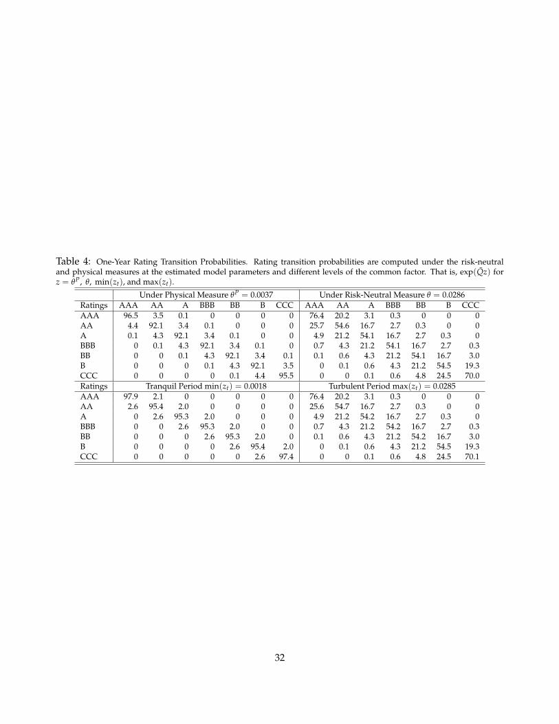
Table 4: One-Year Rating Transition Probabilities. Rating transition probabilities are computed under the risk-neutraland physical measures at the estimated model parameters and different levels of the common factor. That is, exp(Qz) forz = θP, θ, min(zt), and max(zt).
Under Physical Measure θP = 0.0037 Under Risk-Neutral Measure θ = 0.0286Ratings AAA AA A BBB BB B CCC AAA AA A BBB BB B CCCAAA 96.5 3.5 0.1 0 0 0 0 76.4 20.2 3.1 0.3 0 0 0AA 4.4 92.1 3.4 0.1 0 0 0 25.7 54.6 16.7 2.7 0.3 0 0A 0.1 4.3 92.1 3.4 0.1 0 0 4.9 21.2 54.1 16.7 2.7 0.3 0BBB 0 0.1 4.3 92.1 3.4 0.1 0 0.7 4.3 21.2 54.1 16.7 2.7 0.3BB 0 0 0.1 4.3 92.1 3.4 0.1 0.1 0.6 4.3 21.2 54.1 16.7 3.0B 0 0 0 0.1 4.3 92.1 3.5 0 0.1 0.6 4.3 21.2 54.5 19.3CCC 0 0 0 0 0.1 4.4 95.5 0 0 0.1 0.6 4.8 24.5 70.0Ratings Tranquil Period min(zt) = 0.0018 Turbulent Period max(zt) = 0.0285AAA 97.9 2.1 0 0 0 0 0 76.4 20.2 3.1 0.3 0 0 0AA 2.6 95.4 2.0 0 0 0 0 25.6 54.7 16.7 2.7 0.3 0 0A 0 2.6 95.3 2.0 0 0 0 4.9 21.2 54.2 16.7 2.7 0.3 0BBB 0 0 2.6 95.3 2.0 0 0 0.7 4.3 21.2 54.2 16.7 2.7 0.3BB 0 0 0 2.6 95.3 2.0 0 0.1 0.6 4.3 21.2 54.2 16.7 3.0B 0 0 0 0 2.6 95.4 2.0 0 0.1 0.6 4.3 21.2 54.5 19.3CCC 0 0 0 0 0 2.6 97.4 0 0 0.1 0.6 4.8 24.5 70.1
32

Table 5: Proportion of Model Implied CDS Spread Due to Rating Transition Risk. For each country and at each maturity,we report the time series average of the ratio |CDS0 − CDS|/CDS, where CDS is the model implied CDS spread and CDS0
is obtained by setting Q ≡ 0 in the CDS pricing formula, given the in-sample estimated values of z and yi. The first columnreports the last-day rating for each country. The average for each rating is computed according to the actual rating when theprice is quoted rather than the last-day rating for each country.
Rating Country 1y 2y 3y 5y 7y 10y MeanAAA Germany 0.443 0.336 0.395 0.025 0.104 0.230 0.256AA Austria 0.298 0.249 0.447 0.043 0.097 0.216 0.225AA Belgium 0.481 0.287 0.178 0.035 0.167 0.273 0.237AA China 0.433 0.238 0.091 0.025 0.085 0.131 0.167AA Czech 0.340 0.240 0.363 0.025 0.106 0.161 0.206AA Japan 0.591 0.515 0.397 0.032 0.170 0.286 0.332AA Qatar 0.382 0.219 0.103 0.034 0.118 0.195 0.175A Chile 0.452 0.205 0.088 0.026 0.086 0.133 0.165A Israel 0.277 0.141 0.066 0.025 0.079 0.122 0.118A Korea 0.301 0.154 0.070 0.025 0.079 0.123 0.125A Malaysia 0.323 0.167 0.075 0.025 0.082 0.127 0.133A Poland 0.220 0.170 0.087 0.022 0.057 0.081 0.106A Slovakia 0.319 0.220 0.334 0.022 0.087 0.129 0.185BBB Brazil 0.111 0.049 0.022 0.017 0.026 0.036 0.044BBB Bulgaria 0.042 0.055 0.018 0.009 0.012 0.015 0.025BBB Colombia 0.161 0.059 0.029 0.025 0.035 0.045 0.059BBB Croatia 0.034 0.034 0.015 0.008 0.010 0.013 0.019BBB Iceland 0.127 0.099 0.066 0.009 0.042 0.074 0.069BBB Italy 0.442 0.327 0.191 0.021 0.106 0.173 0.210BBB Mexico 0.023 0.014 0.011 0.009 0.010 0.017 0.014BBB Panama 0.163 0.070 0.029 0.024 0.035 0.044 0.061BBB Peru 0.136 0.055 0.024 0.018 0.028 0.036 0.050BBB Russia 0.023 0.016 0.011 0.010 0.012 0.017 0.015BBB South Africa 0.017 0.016 0.011 0.009 0.009 0.016 0.013BBB Thailand 0.062 0.029 0.015 0.009 0.011 0.018 0.024BB Hungary 0.189 0.161 0.055 0.011 0.032 0.052 0.083BB Indonesia 0.265 0.093 0.035 0.039 0.048 0.057 0.089BB Philippines 0.115 0.052 0.029 0.028 0.036 0.047 0.051BB Portugal 0.401 0.339 0.148 0.019 0.102 0.172 0.197BB Romania 0.121 0.126 0.033 0.020 0.026 0.030 0.059BB Turkey 0.103 0.050 0.028 0.027 0.035 0.045 0.048B Ukraine 0.152 0.065 0.036 0.031 0.049 0.074 0.068B Venezuela 0.146 0.079 0.024 0.030 0.044 0.051 0.062CCC Greece 0.173 0.285 0.250 0.023 0.084 0.126 0.157— AAA 0.370 0.295 0.429 0.034 0.099 0.222 0.241— AA 0.543 0.407 0.247 0.030 0.158 0.265 0.275— A 0.330 0.206 0.159 0.024 0.087 0.133 0.156— BBB 0.025 0.027 0.017 0.010 0.010 0.016 0.018— BB 0.143 0.070 0.030 0.026 0.037 0.044 0.058— B 0.368 0.123 0.045 0.044 0.063 0.083 0.121— CCC 0.174 0.144 0.030 0.059 0.113 0.168 0.115— Overall 0.221 0.142 0.108 0.022 0.061 0.097 0.109
33

Table 6: Estimated Standard Deviations of Pricing Errors σjM Across Countries and Maturities. The first column reports thelast-day rating for each country. The average for each rating is computed according to the last-day rating for each country.The sample consists of monthly observations between January 2004 and March 2012.
Rating Country 1y 2y 3y 5y 7y 10yAAA Germany 9.2 7.3 4.6 5.2 7.3 9.7AA Austria 10.6 8.1 5.8 7.4 7.9 12.6AA Belgium 15.2 9.9 9.6 6.4 10.0 17.1AA China 14.3 9.3 5.6 6.3 10.1 13.1AA Czech 13.1 6.8 3.4 5.5 7.3 10.9AA Japan 13.9 9.0 5.0 6.3 9.9 12.2AA Qatar 13.0 7.2 3.9 5.8 7.3 11.4A Chile 12.2 7.3 3.0 6.2 7.7 8.9A Israel 17.7 8.6 3.4 8.3 9.3 11.7A Korea 14.1 10.0 5.7 6.7 10.6 12.6A Malaysia 13.1 9.6 4.5 6.9 8.5 13.1A Poland 28.2 12.9 5.7 9.2 15.8 21.1A Slovakia 16.5 9.9 4.8 5.6 10.4 15.9BBB Brazil 70.4 34.6 15.4 25.0 38.7 51.3BBB Bulgaria 31.3 13.6 7.4 10.9 15.9 24.5BBB Colombia 63.4 38.4 15.9 24.7 38.2 50.3BBB Croatia 35.7 15.4 8.8 11.1 18.3 28.3BBB Iceland 76.1 40.7 7.3 20.4 40.5 54.5BBB Italy 20.7 8.4 5.6 9.0 10.1 11.3BBB Mexico 20.3 11.8 8.0 6.4 11.9 21.8BBB Panama 39.0 23.9 13.8 12.7 24.2 39.1BBB Peru 49.8 31.9 13.4 19.3 31.6 42.1BBB Russia 51.4 21.2 8.5 23.3 27.9 25.4BBB South Africa 23.5 14.0 7.5 9.0 13.2 23.1BBB Thailand 18.3 11.0 5.6 6.4 11.8 16.9BB Hungary 37.3 16.5 7.1 14.3 19.4 25.4BB Indonesia 36.8 27.3 16.8 11.4 25.7 42.8BB Philippines 68.8 42.9 20.4 27.0 41.5 60.9BB Portugal 78.8 90.1 43.7 35.8 71.0 90.2BB Romania 36.7 21.1 11.8 15.0 23.0 32.0BB Turkey 44.6 27.1 14.6 15.2 26.9 41.3B Ukraine 142.2 76.2 37.8 49.7 75.2 112.0B Venezuela 102.9 53.3 32.5 35.4 53.1 80.1CCC Greece 686.3 170.8 65.7 213.2 282.7 309.6Average AAA 9.2 7.3 4.6 5.2 7.3 9.7Average AA 13.4 8.4 5.5 6.3 8.7 12.9Average A 17.0 9.7 4.5 7.2 10.4 13.9Average BBB 41.7 22.1 9.8 14.8 23.5 32.4Average BB 50.5 37.5 19.1 19.8 34.6 48.8Average B 122.5 64.7 35.1 42.6 64.2 96.0Overall Mean 56.6 26.7 12.7 20.0 30.1 39.8Overall SD 115.2 32.2 13.4 35.7 48.0 53.7Overall Min 9.2 6.8 3.0 5.2 7.3 8.9Overall Med 29.7 13.8 7.4 10.0 15.8 23.8Overall Max 686.3 170.8 65.7 213.2 282.7 309.6
34

Table 7: Mean Absolute Pricing Error Relative to Bid-Ask Spread for In-Sample and Out-of-Sample Countries. We alsoreport the last-day rating for each country. The average for each rating is computed according to the actual rating whenthe price is quoted rather than the last-day rating for each country. The sample consists of monthly observations betweenJanuary 2004 and March 2012.
In-Sample Countries Out-of-Sample CountriesRating Country 1y 2y 3y 5y 7y 10y Rating Country 1y 2y 3y 5y 7y 10yAAA Germany 3.2 2.3 1.2 1.2 1.8 2.4 AAA Australia 0.9 0.5 0.4 1.0 0.7 1.0AA Austria 1.7 1.3 0.7 1.1 1.3 1.8 AAA Denmark 1.8 0.8 0.5 0.9 1.0 1.4AA Belgium 1.4 0.9 1.0 0.8 1.2 2.2 AAA Finland 2.7 1.0 0.5 1.0 1.0 1.3AA China 2.1 1.7 0.9 1.3 1.7 2.2 AAA Hong Kong 0.7 0.6 0.4 0.4 0.9 1.2AA Czech 1.0 0.7 0.5 0.7 1.3 2.2 AAA Netherlands 1.7 1.0 0.5 0.9 1.1 1.4AA Japan 4.5 2.2 1.1 1.2 2.0 2.4 AAA Norway 1.2 1.0 0.6 0.7 0.8 1.2AA Qatar 0.9 0.6 0.3 0.6 0.7 1.0 AAA Sweden 2.1 1.3 0.5 1.1 1.1 1.4A Chile 1.0 0.6 0.2 0.5 0.6 0.7 AAA Switzerland 1.0 0.8 0.4 0.7 0.9 0.8A Israel 1.4 0.7 0.3 0.7 0.8 1.0 AAA UK 4.5 2.8 1.2 2.0 1.9 1.8A Korea 1.5 1.1 0.7 0.8 1.4 1.8 AA Abu Dhabi 1.8 1.3 0.6 0.8 1.1 2.0A Malaysia 2.1 1.4 0.6 1.0 1.2 1.7 AA Estonia 1.7 0.8 0.5 0.9 1.2 1.6A Poland 2.7 1.3 0.8 2.0 2.9 3.9 AA France 2.7 1.8 0.8 1.6 1.6 1.8A Slovakia 0.8 0.8 0.6 0.8 1.5 2.4 AA New Zealand 0.5 0.7 0.9 0.4 0.9 2.3BBB Brazil 4.2 2.9 1.5 2.6 3.0 5.0 AA Saudi Arabia 0.5 0.5 0.2 0.4 0.6 1.1BBB Bulgaria 1.8 1.1 0.5 1.2 1.8 2.5 AA USA 0.7 0.7 0.6 0.5 0.9 1.5BBB Colombia 3.6 2.2 1.1 1.6 2.5 3.5 A Slovenia 1.5 0.8 0.3 0.9 1.0 1.2BBB Croatia 1.4 0.9 0.5 0.9 1.5 2.1 A Spain 1.9 1.5 1.3 1.6 1.8 2.8BBB Iceland 0.7 0.7 0.3 0.5 1.2 1.8 BBB Bahrain 0.8 0.4 0.3 0.7 0.6 1.1BBB Italy 1.7 1.0 0.8 1.4 1.4 1.8 BBB Ireland 1.0 1.2 1.1 1.2 2.2 3.1BBB Mexico 2.5 1.5 1.0 1.4 1.7 2.9 BBB Kazakhstan 2.4 0.9 0.4 1.3 1.4 2.0BBB Panama 1.8 1.0 0.6 0.7 1.3 2.1 BBB Lithuania 1.5 1.0 0.5 0.8 1.6 2.5BBB Peru 2.3 1.3 0.7 1.0 1.5 2.5 BBB Morocco 0.8 0.6 0.3 0.3 1.0 1.5BBB Russia 3.7 1.4 0.7 2.4 2.6 3.3 BB Costa Rica 1.0 1.0 0.7 0.3 1.0 1.7BBB South Africa 2.4 1.4 0.6 1.3 1.5 2.3 BB Cyprus 0.8 1.0 0.7 1.1 2.0 2.9BBB Thailand 1.7 1.4 0.6 1.0 1.5 2.1 BB El Salvador 1.1 0.5 0.3 0.6 0.7 1.2BB Hungary 2.2 1.2 0.6 1.7 2.1 2.9 BB Guatemala 0.7 0.6 0.3 0.3 0.7 0.9BB Indonesia 1.5 1.2 1.3 0.9 1.3 2.5 BB Latvia 1.5 1.2 0.6 1.2 1.9 2.4BB Philippines 2.8 2.2 1.6 2.0 2.2 3.7 BB Vietnam 1.1 0.8 0.4 0.8 1.3 1.7BB Portugal 1.1 0.9 0.8 1.0 1.7 2.2 B Argentina 2.9 1.7 1.1 1.7 2.3 3.9BB Romania 1.8 1.4 0.6 1.3 2.4 3.4 B Dominican 0.2 0.1 0.1 0.1 0.1 0.3BB Turkey 4.1 3.4 1.9 2.5 3.6 6.2 B Ecuador 4.0 2.5 1.1 2.6 4.9 7.3B Ukraine 1.9 1.7 1.1 1.3 2.1 3.6 B Egypt 1.0 0.7 0.5 0.6 1.1 1.6B Venezuela 2.4 1.7 1.0 1.6 2.5 4.0 B Lebanon 1.6 1.0 0.9 1.0 1.6 2.1CCC Greece 1.4 1.2 0.6 2.0 3.0 3.4 B Pakistan 1.3 0.8 0.5 0.5 1.1 1.2— AAA 2.4 1.7 0.9 1.1 1.5 2.1 — AAA 1.2 0.9 0.5 0.7 1.1 1.6— AA 2.3 1.3 0.8 0.9 1.3 1.9 — AA 1.6 1.2 0.8 1.1 1.7 2.6— A 1.4 0.9 0.5 0.9 1.3 1.7 — A 1.5 1.0 0.6 0.9 1.4 2.1— BBB 2.2 1.3 0.7 1.4 2.0 2.9 — BBB 1.5 0.8 0.5 0.9 1.0 1.4— BB 2.7 2.1 1.3 1.7 2.4 4.0 — BB 2.1 1.3 0.6 1.1 1.3 1.7— B 2.5 1.2 0.7 1.4 2.0 2.8 — B 0.8 0.7 0.7 0.4 0.9 1.5— CCC 1.7 1.0 0.4 2.0 2.9 3.4 — CCC 0.4 0.4 0.5 0.4 0.3 1.1— Overall 2.1 1.4 0.8 1.3 1.8 2.6 — Overall 1.6 1.0 0.6 1.0 1.3 1.8
35

Table 8: OLS Regression of Observed 5-Year CDS Spreads on CDS Spreads Implied by the z-Only Model. We obtain the z-only model by setting the country-specific factors to zero in Model I estimated using the 34 in-sample countries. The averagefor each rating is computed according to the last-day rating for each country. The sample consists of monthly observationsbetween January 2004 and March 2012.
In-Sample Countries Out-of-Sample CountriesRating Country β t-stat. R2 Rating Country β t-stat. R2
AAA Germany 1.27 11.9 0.59 AAA Australia 1.36 10.0 0.70AA Austria 2.88 16.9 0.75 AAA Denmark 1.86 11.4 0.70AA Belgium 2.08 9.0 0.46 AAA Finland 0.95 9.4 0.62AA China 0.73 10.5 0.53 AAA Hong Kong 1.26 13.7 0.69AA Czech 1.08 16.6 0.74 AAA Netherlands 1.55 11.5 0.68AA Japan 1.04 9.4 0.48 AAA Norway 0.53 8.1 0.58AA Qatar 2.11 12.5 0.63 AAA Sweden 1.50 11.8 0.71A Chile 0.98 26.7 0.89 AAA Switzerland 1.49 7.1 0.58A Israel 1.02 19.6 0.81 AAA UK 1.49 8.8 0.58A Korea 1.52 20.2 0.81 AA Abu Dhabi 1.54 4.5 0.38A Malaysia 1.08 22.6 0.84 AA Estonia 2.61 13.7 0.78A Poland 1.37 11.3 0.57 AA France 2.02 8.5 0.48A Slovakia 1.01 11.8 0.60 AA New Zealand 1.12 9.4 0.70BBB Brazil 0.79 7.3 0.36 AA Saudi Arabia 1.45 7.8 0.66BBB Bulgaria 1.20 26.0 0.87 AA USA 0.59 6.7 0.45BBB Colombia 0.16 2.6 0.07 A Slovenia 2.36 8.8 0.62BBB Croatia 1.23 24.2 0.86 A Spain 2.73 7.2 0.45BBB Iceland 1.67 15.2 0.71 BBB Bahrain 0.75 5.5 0.41BBB Italy 1.41 13.1 0.64 BBB Ireland 2.10 10.9 0.68BBB Mexico 0.56 15.1 0.70 BBB Kazakhstan 1.51 10.0 0.56BBB Panama 0.31 9.1 0.46 BBB Lithuania 1.11 12.8 0.73BBB Peru 0.48 5.4 0.24 BBB Morocco 0.23 6.7 0.53BBB Russia 1.24 16.9 0.76 BB Costa Rica 0.33 10.8 0.77BBB South Africa 0.73 19.8 0.80 BB Cyprus 2.95 30.6 0.99BBB Thailand 0.55 27.5 0.89 BB El Salvador 0.51 15.2 0.88BB Hungary 1.08 23.4 0.85 BB Guatemala -0.19 -1.8 0.13BB Indonesia 0.48 9.2 0.49 BB Latvia 0.77 6.4 0.42BB Philippines 0.06 0.9 0.01 BB Vietnam 0.55 20.2 0.83BB Portugal 2.79 22.6 0.84 B Argentina 1.65 11.3 0.62BB Romania 0.68 30.5 0.91 B Dominican -0.12 -0.7 0.07BB Turkey 0.25 6.4 0.31 B Ecuador 0.73 12.3 0.90B Ukraine 0.67 17.5 0.77 B Egypt 0.43 10.3 0.69B Venezuela 1.03 6.3 0.30 B Lebanon 0.15 6.0 0.42CCC Greece 1.28 40.2 0.94 B Pakistan 0.51 26.0 0.90Average AAA 1.27 11.9 0.59 Average AAA 1.33 10.2 0.65Average AA 1.65 12.5 0.60 Average AA 1.55 8.4 0.58Average A 1.16 18.7 0.75 Average A 2.54 8.0 0.54Average BBB 0.86 15.2 0.61 Average BBB 1.14 9.2 0.58Average BB 0.89 15.5 0.57 Average BB 0.82 13.6 0.67Average B 0.85 11.9 0.54 Average B 0.56 10.9 0.60Overall Mean 1.08 15.8 0.63 Overall Mean 1.19 10.3 0.61Overall SD 0.66 8.7 0.25 Overall SD 0.81 6.2 0.20Overall Min 0.06 0.9 0.01 Overall Min -0.19 -1.8 0.07Overall Med 1.04 15.2 0.71 Overall Med 1.19 9.7 0.64Overall Max 2.88 40.2 0.94 Overall Max 2.95 30.6 0.99
36

Tabl
e9:
OLS
Reg
ress
ion
ofth
eEs
tim
ated
Com
mon
Fact
orz
(in
perc
ent)
,the
Mar
ket
Pric
eof
Ris
kλ(t
),an
dth
e5-
year
Cre
dit
Ris
kPr
emiu
mon
the
CBO
EV
IXin
dex,
the
5-Ye
arU
STr
easu
ryR
ate,
and
the
CD
XN
AIG
Inde
x.t-
stat
isti
csar
ere
port
edin
squa
red
brac
kets
.Int
cst
ands
for
Inte
rcep
t.Tr
eas
repr
esen
tsTr
easu
re.
Com
mon
Fact
orz
Pric
eof
Ris
kλ(t
)R
isk
Prem
ium
CR
P(5
)In
tcV
IXTr
eas
CD
XR
2 (%
)In
tcV
IXTr
eas
CD
XR
2 (%
)In
tcV
IXTr
eas
CD
XR
2 (%
)-0
.22
5.02
62.3
50.
84-1
0.92
56.3
6-0
.68
4.08
57.9
0[-2
.36]
[12.
68]
[3.6
7][-1
1.19
][-8
.20]
[11.
55]
2.07
-40.
4261
.70
-4.6
510
4.83
79.3
71.
32-3
7.58
75.1
0[1
9.40
][-1
2.50
][-2
6.00
][1
9.32
][1
8.30
][-1
7.11
]-0
.22
1.21
74.0
50.
98-2
.81
76.0
6-0
.72
1.03
76.1
7[-3
.01]
[16.
64]
[6.2
4][-
17.5
5][-
12.4
3][1
7.61
]0.
943.
19-2
5.32
78.3
1-2
.85
-5.0
880
.80
87.4
20.
592.
07-2
7.79
84.9
5[6
.06]
[8.5
7][-
8.40
][-1
0.59
][-7
.84]
[15.
40]
[5.4
5][7
.92
[-13.
13]
0.66
1.22
-19.
190.
5980
.28
-2.0
60.
4463
.68
-1.6
490
.37
0.30
0.04
-21.
480.
6087
.89
[3.7
7][1
.66]
[-5.
48]
[3.0
8][-
7.43
][0
.38]
[11.
36]
[-5.3
9][2
.63]
[0.0
8][-
9.28
][4
.81]
Tabl
e10
:OLS
Reg
ress
ion
ofth
eEs
tim
ated
Com
mon
Fact
orz
(in
perc
ent)
,the
Mar
ketP
rice
ofD
efau
ltR
isk
λ(t
),an
dth
e5-
year
Cre
ditR
isk
Prem
ium
onth
eC
BOE
VIX
Inde
x,th
e5-
Year
US
Trea
sury
Rat
e,th
eR
etur
non
the
MSC
IWor
ldSt
ock
Mar
ketI
ndex
,the
Ret
urn
onth
eS&
P50
0In
dex,
the
Ret
urn
onth
eD
AX
Inde
x,an
dth
eC
DX
NA
IGIn
dex.
t-st
atis
tics
are
repo
rted
insq
uare
dbr
acke
ts.
Inte
rcep
tV
IXTr
easu
reC
DX
MSC
IS&
P50
0D
AX
R2 (
%)
NC
omm
onFa
ctor
z t0.
701.
26-2
0.29
0.56
-0.7
1-1
.02
1.63
80.8
199
[3.6
6][1
.59]
[-5.
48]
[2.9
1][-
0.27
][-
0.35
][1
.58]
Pric
eof
Ris
kλ(t
)-2
.11
0.46
64.4
5-1
.61
4.44
-2.2
3-2
.05
90.5
999
[-6.
91]
[0.3
6][1
0.88
][-
5.24
][1
.05]
[-0.
48]
[-1.
24]
Ris
kPr
emiu
mC
RP(5
)0.
35-0
.01
-22.
380.
59-1
.15
-0.3
51.
2388
.35
99[2
.79]
[-0.
02]
[-9.
21]
[4.6
7][-
0.66
][-
0.18
][1
.82]
37
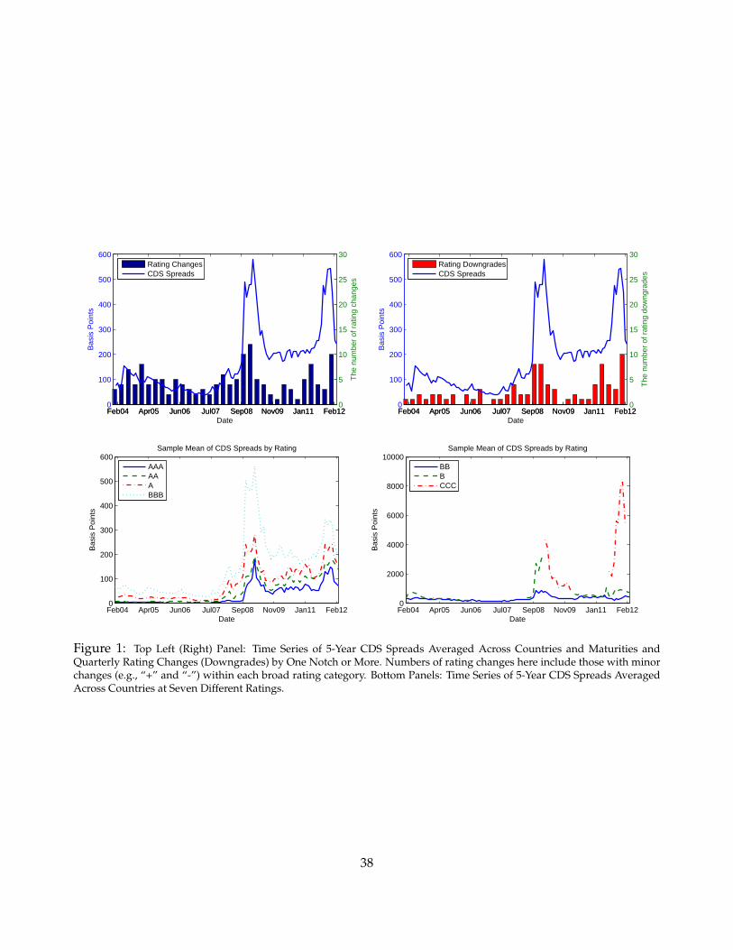
Feb04 Apr05 Jun06 Jul07 Sep08 Nov09 Jan11 Feb120
100
200
300
400
500
600
Bas
is P
oint
s
Date
Feb04 Apr05 Jun06 Jul07 Sep08 Nov09 Jan11 Feb120
5
10
15
20
25
30
The
num
ber
of r
atin
g ch
ange
s
Rating ChangesCDS Spreads
Feb04 Apr05 Jun06 Jul07 Sep08 Nov09 Jan11 Feb120
100
200
300
400
500
600
Bas
is P
oint
s
Date
Feb04 Apr05 Jun06 Jul07 Sep08 Nov09 Jan11 Feb120
5
10
15
20
25
30
The
num
ber
of r
atin
g do
wng
rade
s
Rating DowngradesCDS Spreads
Feb04 Apr05 Jun06 Jul07 Sep08 Nov09 Jan11 Feb120
100
200
300
400
500
600
Date
Bas
is P
oint
s
Sample Mean of CDS Spreads by Rating
AAAAAABBB
Feb04 Apr05 Jun06 Jul07 Sep08 Nov09 Jan11 Feb120
2000
4000
6000
8000
10000
Date
Bas
is P
oint
s
Sample Mean of CDS Spreads by Rating
BBBCCC
Figure 1: Top Left (Right) Panel: Time Series of 5-Year CDS Spreads Averaged Across Countries and Maturities andQuarterly Rating Changes (Downgrades) by One Notch or More. Numbers of rating changes here include those with minorchanges (e.g., “+” and “-”) within each broad rating category. Bottom Panels: Time Series of 5-Year CDS Spreads AveragedAcross Countries at Seven Different Ratings.
38

Feb04 Apr05 Jun06 Jul07 Sep08 Nov09 Dec10 Feb120
20
40
60
80
100
120
BBBBBB+
BBBBBB−
BB+n
Bulgaria (BBB)
Feb04 Apr05 Jun06 Jul07 Sep08 Nov09 Dec10 Feb120
10
20
30
40
50
60
A+A
Chile (A+)
Feb04 Apr05 Jun06 Jul07 Sep08 Nov09 Dec10 Feb120
50
100
150BBB−
BBB
BBB−
Croatia (BBB−)
Feb04 Apr05 Jun06 Jul07 Sep08 Nov09 Dec10 Feb120
10
20
30
40
50
AA−A
A−
Czech Republic (AA−)
Feb04 Apr05 Jun06 Jul07 Sep08 Nov09 Dec10 Feb120
50
100
150
200
250
300
350
BBB−BBB
A−A
A+
AA−A+
nnnn
Iceland (BBB−)
Feb04 Apr05 Jun06 Jul07 Sep08 Nov09 Dec10 Feb120
50
100
150 BB+BB
BB−B+
B
Indonesia (BB+)
Feb04 Apr05 Jun06 Jul07 Sep08 Nov09 Dec10 Feb120
10
20
30
40
50
60
70A+
A
A−
Israel (A+)
Feb04 Apr05 Jun06 Jul07 Sep08 Nov09 Dec10 Feb120
10
20
30
40
50
AA−
Korea (A)
Feb04 Apr05 Jun06 Jul07 Sep08 Nov09 Dec10 Feb120
10
20
30
40
50
60
Malaysia (A−)
Feb04 Apr05 Jun06 Jul07 Sep08 Nov09 Dec10 Feb120
20
40
60
80
100BBB−
BB+
BB
Panama (BBB−)
Feb04 Apr05 Jun06 Jul07 Sep08 Nov09 Dec10 Feb120
10
20
30
40
50
60
AAAA−
A+
Qatar (AA)
Feb04 Apr05 Jun06 Jul07 Sep08 Nov09 Dec10 Feb120
20
40
60
80
100
120
BB+BBB−
BB+BB
Romania (BB+)
Feb04 Apr05 Jun06 Jul07 Sep08 Nov09 Dec10 Feb120
50
100
150
BBBBBB+
BBBBBB−
BB+
Russia (BBB)
Feb04 Apr05 Jun06 Jul07 Sep08 Nov09 Dec10 Feb120
10
20
30
40
50
60
70A
A+
AA−
BBB+
BBB
n
Slovakia (A)
Feb04 Apr05 Jun06 Jul07 Sep08 Nov09 Dec10 Feb120
20
40
60
80
100BBB+
BBB
South Africa (BBB+)
Feb04 Apr05 Jun06 Jul07 Sep08 Nov09 Dec10 Feb120
10
20
30
40
50
60
70BBB+
BBBn
Thailand (BBB+)
Feb04 Apr05 Jun06 Jul07 Sep08 Nov09 Dec10 Feb120
100
200
300
400
500B+
B
B−CCC+
B
B+BB−
B+
B
pnn
Ukraine (B+)
Figure 2: Time Series of Absolute Pricing Errors (dash-dot lines) and Bid-Ask Spreads (solid lines) Averaged Across Ma-turities for In-sample Non-Eurozone Countries with Low Pricing Errors. “SD” is for Selective Default, “n” is for negativeCredit Watch, “p” is for positive Credit Watch. Vertical lines represent the dates of credit rating changes for each country.
39

Feb04 Apr05 Jun06 Jul07 Sep08 Nov09 Dec10 Feb120
10
20
30
40
50
60
Abu Dhabi (AA)
Feb04 Apr05 Jun06 Jul07 Sep08 Nov09 Dec10 Feb120
200
400
600
800
BB−
BB+
B
B−SD
Argentina (B)
Feb04 Apr05 Jun06 Jul07 Sep08 Nov09 Dec10 Feb120
5
10
15
20
25
30
35
Australia (AAA)
Feb04 Apr05 Jun06 Jul07 Sep08 Nov09 Dec10 Feb120
50
100
150BBBA−
AA−
nn
Bahrain (BBB)
Feb04 Apr05 Jun06 Jul07 Sep08 Nov09 Dec10 Feb120
50
100
150BB+
BB
Costa Rica (BB+)
Feb04 Apr05 Jun06 Jul07 Sep08 Nov09 Dec10 Feb120
10
20
30
40
50
60
70BB+
BBB
BBB+A−
A
A+A
nnn
Cyprus (BB+)
Feb04 Apr05 Jun06 Jul07 Sep08 Nov09 Dec10 Feb120
5
10
15
20
25
30
35
Denmark (AAA)
Feb04 Apr05 Jun06 Jul07 Sep08 Nov09 Dec10 Feb120
20
40
60
80
100
120
140
B+B
B+B
SD
CCCCC
n
Dominican Republic (B+)
Feb04 Apr05 Jun06 Jul07 Sep08 Nov09 Dec10 Feb120
200
400
600
800B−
CCC+
SDCCC−
B−
CCCCCC+
B−
CCC+
nnn
Ecuador (B−)
Feb04 Apr05 Jun06 Jul07 Sep08 Nov09 Dec10 Feb120
50
100
150
200
BB+
BB−BB
BB+n
Egypt (B)
Feb04 Apr05 Jun06 Jul07 Sep08 Nov09 Dec10 Feb120
20
40
60
80
100BB−
BB
BB+
El Salvador (BB−)
Feb04 Apr05 Jun06 Jul07 Sep08 Nov09 Dec10 Feb120
50
100
150AA−
A
A−A
A−nn
Estonia (AA−)
Feb04 Apr05 Jun06 Jul07 Sep08 Nov09 Dec10 Feb120
50
100
150
BBBB−
Guatemala (BB)
Feb04 Apr05 Jun06 Jul07 Sep08 Nov09 Dec10 Feb120
10
20
30
40
50
AAAAA+
AAAA−
A+
Hong Kong (AAA)
Feb04 Apr05 Jun06 Jul07 Sep08 Nov09 Dec10 Feb120
50
100
150
200
BBB+BBB
BBB−BBB
BBB−
BB+
n
Kazakhstan (BBB+)
Figure 3: Time Series of Absolute Pricing Errors (dash-dot lines) and Bid-Ask Spreads (solid lines) Averaged Across Matu-rities for Out-of-Sample Non-Eurozone Countries. “SD” is for Selective Default, “n” is for negative Credit Watch, “p” is forpositive Credit Watch. Vertical lines represent the dates of credit rating changes for each country.
40

Feb04 Apr05 Jun06 Jul07 Sep08 Nov09 Dec10 Feb120
50
100
150
200
250
BB+BB
BB+BBB−BBB
BBB+A−
BBB+nn
Latvia (BB+)
Feb04 Apr05 Jun06 Jul07 Sep08 Nov09 Dec10 Feb120
50
100
150 BB−
CCC+B−
nn
Lebanon (B)
Feb04 Apr05 Jun06 Jul07 Sep08 Nov09 Dec10 Feb120
50
100
150BBB
BBB+
A−A
A−
BBB+
nnn
Lithuania (BBB)
Feb04 Apr05 Jun06 Jul07 Sep08 Nov09 Dec10 Feb120
50
100
150 BBB−BB+
BB
Morocco (BBB−)
Feb04 Apr05 Jun06 Jul07 Sep08 Nov09 Dec10 Feb120
5
10
15
20
25
30
35AA
AA+
New Zealand (AA)
Feb04 Apr05 Jun06 Jul07 Sep08 Nov09 Dec10 Feb120
5
10
15
20
25
Norway (AAA)
Feb04 Apr05 Jun06 Jul07 Sep08 Nov09 Dec10 Feb120
500
1000
1500
2000
2500B−
CCC+
CCCCCC+
B
B+B
Pakistan (B−)
Feb04 Apr05 Jun06 Jul07 Sep08 Nov09 Dec10 Feb120
20
40
60
80AA−
A+
A
Saudi Arabia (AA−)
Feb04 Apr05 Jun06 Jul07 Sep08 Nov09 Dec10 Feb120
10
20
30
40
50
60
70A+
AA−
AAAA−
A+n
Slovenia (A+)
Feb04 Apr05 Jun06 Jul07 Sep08 Nov09 Dec10 Feb120
5
10
15
20
25
30
35AAAAA+
Sweden (AAA)
Feb04 Apr05 Jun06 Jul07 Sep08 Nov09 Dec10 Feb120
5
10
15
20
25
30
35
Switzerland (AAA)
Feb04 Apr05 Jun06 Jul07 Sep08 Nov09 Dec10 Feb120
5
10
15
20
25
AA+AAA
n
USA (AA+)
Feb04 Apr05 Jun06 Jul07 Sep08 Nov09 Dec10 Feb120
20
40
60
80
100
120
BB−BB
BB−
Vietnam (BB−)
Figure 3: (Continued)
41
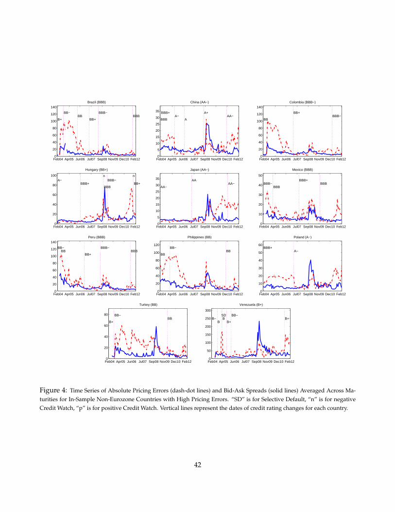
Feb04 Apr05 Jun06 Jul07 Sep08 Nov09 Dec10 Feb120
20
40
60
80
100
120
140
BBBBBB−
BB+BB
BB−
B+
Brazil (BBB)
Feb04 Apr05 Jun06 Jul07 Sep08 Nov09 Dec10 Feb120
5
10
15
20
25
30
35AA−
A+
AA−
BBB+
BBB
China (AA−)
Feb04 Apr05 Jun06 Jul07 Sep08 Nov09 Dec10 Feb120
20
40
60
80
100
120
140
BBB−BB+
BB
Colombia (BBB−)
Feb04 Apr05 Jun06 Jul07 Sep08 Nov09 Dec10 Feb120
20
40
60
80
100
BB+BBB−
BBBBBB+
A−nn
Hungary (BB+)
Feb04 Apr05 Jun06 Jul07 Sep08 Nov09 Dec10 Feb120
5
10
15
20
25
30
35AA−
AA
AA−
Japan (AA−)
Feb04 Apr05 Jun06 Jul07 Sep08 Nov09 Dec10 Feb120
10
20
30
40
50
BBBBBB+
BBBBBB−
Mexico (BBB)
Feb04 Apr05 Jun06 Jul07 Sep08 Nov09 Dec10 Feb120
20
40
60
80
100
120
140
BBBBBB−
BB+BB
BB−
Peru (BBB)
Feb04 Apr05 Jun06 Jul07 Sep08 Nov09 Dec10 Feb120
20
40
60
80
100
120
BBBB−
BB
Philippines (BB)
Feb04 Apr05 Jun06 Jul07 Sep08 Nov09 Dec10 Feb120
10
20
30
40
50
60
A−BBB+
Poland (A−)
Feb04 Apr05 Jun06 Jul07 Sep08 Nov09 Dec10 Feb120
20
40
60
80BB
BB−
B+
Turkey (BB)
Feb04 Apr05 Jun06 Jul07 Sep08 Nov09 Dec10 Feb120
50
100
150
200
250
300
B+BB−
B+B
SD
BB−
Venezuela (B+)
Figure 4: Time Series of Absolute Pricing Errors (dash-dot lines) and Bid-Ask Spreads (solid lines) Averaged Across Ma-turities for In-Sample Non-Eurozone Countries with High Pricing Errors. “SD” is for Selective Default, “n” is for negativeCredit Watch, “p” is for positive Credit Watch. Vertical lines represent the dates of credit rating changes for each country.
42

1 2 3 5 7 10−30
−20
−10
0
10
20China
Time to Maturity
Pric
ing
Err
or (
bps)
pre−changepost−change
1 2 3 5 7 10−40
−30
−20
−10
0
10
20
30Poland
Time to Maturity
Pric
ing
Err
or (
bps)
pre−changepost−change
Figure 5: Changes in CDS Pricing Errors Across Maturities for China and Poland Around Rating Upgrades. China andPoland were upgraded to A- from BBB+ on July 20, 2005 and March 29, 2007, respectively.
Feb04 Apr05 Jun06 Jul07 Sep08 Nov09 Dec10 Feb120
5
10
15
20
25
30
35AA+
AAAn
Austria (AA+)
Feb04 Apr05 Jun06 Jul07 Sep08 Nov09 Dec10 Feb120
10
20
30
40
50
AAAA+
n
Belgium (AA)
Feb04 Apr05 Jun06 Jul07 Sep08 Nov09 Dec10 Feb120
5
10
15
20
25
30
35n
Germany (AAA)
Feb04 Apr05 Jun06 Jul07 Sep08 Nov09 Dec10 Feb120
500
1000
1500
2000
2500
SDCC
CCCB
BB−
BB+BBB+
A−
AA+
nnnnnn
Greece (SD)
Feb04 Apr05 Jun06 Jul07 Sep08 Nov09 Dec10 Feb120
10
20
30
40
50
60
BBB+A
A+AA−
AAn
Italy (BBB+)
Feb04 Apr05 Jun06 Jul07 Sep08 Nov09 Dec10 Feb120
50
100
150
200
250
300
350
BBBBB−
BBBA−
A+
AA−AA
nnnn
Portugal (BB)
Figure 6: Time Series of Absolute Pricing Errors (dash-dot lines) and Bid-Ask Spreads (solid lines) Averaged Across Ma-turities for In-Sample Eurozone Countries. “SD” is for Selective Default, “n” is for negative Credit Watch, “p” is for positiveCredit Watch. Vertical lines represent the dates of credit rating changes for each country.
43

Feb04 Apr05 Jun06 Jul07 Sep08 Nov09 Dec10 Feb120
5
10
15
20
25 n
Finland (AAA)
Feb04 Apr05 Jun06 Jul07 Sep08 Nov09 Dec10 Feb120
5
10
15
20
25
30
35AA+
AAAn
France (AA+)
Feb04 Apr05 Jun06 Jul07 Sep08 Nov09 Dec10 Feb120
50
100
150
200
BBB+A−
AAA−
AA
AA+AAA
nnn
Ireland (BBB+)
Feb04 Apr05 Jun06 Jul07 Sep08 Nov09 Dec10 Feb120
5
10
15
20
25
30
35n
Netherlands (AAA)
Feb04 Apr05 Jun06 Jul07 Sep08 Nov09 Dec10 Feb120
10
20
30
40
50
60
70A
AA−
AAAA+
AAA
AA+
nn
Spain (A)
Feb04 Apr05 Jun06 Jul07 Sep08 Nov09 Dec10 Feb120
5
10
15
20
25
30
35
United Kingdom (AAA)
Figure 7: Time Series of Absolute Pricing Errors (dash-dot lines) and Bid-Ask Spreads (solid lines) Averaged Across Ma-turities for Out-of-Sample Eurozone Countries. “SD” is for Selective Default, “n” is for negative Credit Watch, “p” is forpositive Credit Watch. Vertical lines represent the dates of credit rating changes for each country.
44

Feb04 Apr05 Jun06 Jul07 Sep08 Nov09 Jan11 Feb12−0.5
0
0.5
1
1.5
2
2.5
3
3.5
Date
The Estimated Global Factor
zt(%)zt
Feb04 Apr05 Jun06 Jul07 Sep08 Nov09 Jan11 Feb12−6
−5
−4
−3
−2
−1
0
1
2
Date
The Price of Risk
λ(t)
λ(t)
Feb04 Apr05 Jun06 Jul07 Sep08 Nov09 Jan11 Feb12−1
−0.5
0
0.5
1
1.5
2
Date
The Credit Risk Premium
CRP(5)
CRP (5)
Figure 8: Time Series of the Estimated zt, the Price of Risk λ(t), and the Average 5-Year Credit Risk Premium. The average5-year CRP is computed by (16) for 5-year CDS contracts over all countries . The hatted time series are the respectivepredicted values based on OLS regressions (with 3 explanatory variables) in Table 9.
45

Feb04 Apr05 Jun06 Jul07 Sep08 Nov09 Jan11 Feb12−1
0
1
2
3
4
5
Date
CRP by Rating
AAAAAABBBBBBCCC
Feb04 Apr05 Jun06 Jul07 Sep08 Nov09 Jan11 Feb12−1
0
1
2
3
4
5
Date
CRP by Maturity
1yr2yr3yr5yr7yr10yr
Figure 9: Average Credit Risk Premium for Different Ratings and Maturities. The average CRP for each rating is computedby (16) over all 6 maturities (1y, 2y, 3y, 5y, 7y, 10y), and the average CRP for each maturity is computed by (16) over all 7ratings. All calculations are based on the estimation of Model I reported in Table 3 with zero country-specific factor.
46