a regularized discriminative framework for eeg …ttic.uchicago.edu/~ryotat/papers/tommue10.pdf ·...

NeuroImage 49 (2010) 415–432

Contents lists available at ScienceDirect

NeuroImage

j ourna l homepage: www.e lsev ie r.com/ locate /yn img

A regularized discriminative framework for EEG analysis with application tobrain–computer interface

Ryota Tomioka a,b,c,⁎, Klaus-Robert Müller c,d

a Department of Mathematical Informatics, University of Tokyo, 7-3-1, Hongo, Bunkyo-ku, Tokyo, 113-8656, Japanb Department of Computer Science, Tokyo Institute of Technology, 2-12-1-W8-74, O-okayama, Meguro-ku, Tokyo, 152-8552, Japanc Machine Learning Group, Department of Computer Science, TU Berlin, Franklinstr. 28/29, 10587 Berlin, Germanyd Bernstein Centers for Neurotechnology and Computational Neuroscience Berlin, Germany

⁎ Corresponding author. Department of MathematiTokyo, 7-3-1, Hongo, Bunkyo-ku, Tokyo, 113-8656, Japa

E-mail addresses: [email protected] (R. T(K.-R. Müller).

1053-8119/$ – see front matter © 2009 Elsevier Inc. Adoi:10.1016/j.neuroimage.2009.07.045

a b s t r a c t
a r t i c l e i n f o
Article history:Received 13 February 2009Revised 7 July 2009Accepted 17 July 2009Available online 29 July 2009

Keywords:Brain–computer interfaceDiscriminative learningRegularizationGroup-lassoSpatio-temporal factorizationDual spectral normTrace normConvex optimizationP300 spellerDiscriminative modeling of brain imagingsignals

We propose a framework for signal analysis of electroencephalography (EEG) that unifies tasks such asfeature extraction, feature selection, feature combination, and classification, which are often independentlytackled conventionally, under a regularized empirical risk minimization problem. The features areautomatically learned, selected and combined through a convex optimization problem. Moreover wepropose regularizers that induce novel types of sparsity providing a new technique for visualizing EEG ofsubjects during tasks from a discriminative point of view. The proposed framework is applied to two typicalBCI problems, namely the P300 speller system and the prediction of self-paced finger tapping. In bothdatasets the proposed approach shows competitive performance against conventional methods, while at thesame time the results are easier accessible to neurophysiological interpretation. Note that our novelapproach is not only applicable to Brain imaging beyond EEG but also to general discriminative modeling ofexperimental paradigms beyond BCI.

© 2009 Elsevier Inc. All rights reserved.

Introduction

Brain–computer interface (BCI) is a rapidly growing field ofresearch combining neurophysiological insights, statistical signalanalysis, and machine learning (Wolpaw et al., 2002; Dornhege etal., 2007; Curran and Stokes, 2003; Kübler et al., 2001; Birbaumer etal., 1999; Penny et al., 2000; Parra et al., 2002; Pfurtscheller et al.,2006; Blankertz et al., 2006a, 2007). The goal of BCI research is to builda communication channel from the brain to computers bypassingperipheral nerves and muscle activity (Wolpaw et al., 2002). This canhelp people who have damage in their peripheral pathway to recovertheir communication abilities (e.g. Birbaumer et al. (1999); Kübler etal. (2001); Nicolelis (2003); Hochberg et al. (2006)).

Among different techniques for the noninvasive measurement ofthe human brain, the electroencephalography (EEG) is commerciallyaffordable and has excellent temporal resolution which enables real-time interaction through BCI. Thus our primary focus in this paper is

cal Informatics, University ofn. Fax: +81 3 5841 6897.omioka), [email protected]

ll rights reserved.

on EEG-based BCI but the techniques presented can also be applied toother brain imaging techniques such as magnetoencephalography(MEG) or fMRI. Note furthermore that discriminative techniques are avaluable tool for a computational analysis of neuroscience experi-ments beyond BCI (e.g. Haynes and Rees (2006); Parra et al. (2005)).

Based on a short segment of EEG called a trial, the signal analysis inBCI aims to predict the brain state of a user out of prescribed options(e.g. foot vs. left-hand motor imagery vs. rest). In machine learningterms, this is a multi-class classification problem. The challenge inEEG-based BCI is the low spatial resolution caused by volumeconduction, the high artifact and outlier content of the signal andthe mass of data that makes the application of conventional statisticalanalysis difficult. Therefore many studies have focused on how toextract a small number of task informative features from the data (seee.g. Dornhege et al. (2007); Blankertz et al. (2008)) that can be fedinto some relatively simple classifiers; commonly used are linearspatial filtering methods (e.g., common spatial pattern (Ramoser etal., 2000; Blankertz et al., 2008) or independent component analysis(Hyvärinen et al., 2001)) coupled with heuristic frequency bandselection (Blankertz et al., 2008) or band weighting (Tomioka et al.,2006b; Wu et al., 2008). One of the shortcomings of the featureextraction approaches is the strong and hard-to-control inductive bias

mailto:[email protected]

mailto:[email protected]

http://dx.doi.org/10.1016/j.neuroimage.2009.07.045

http://www.sciencedirect.com/science/journal/10538119

416 R. Tomioka, K.-R. Müller / NeuroImage 49 (2010) 415–432

that limits their application to rather specific experimental paradigmsthat they are developed for. Another approach is the discriminativeapproach that tries to optimize the classifier coefficients from thetraining data under a unified criterion(Dyrholm and Parra, 2006;Dyrholm et al., 2007; Christoforou et al., 2008; Farquhar et al., 2006;Tomioka et al., 2007; Tomioka and Aihara, 2007). The theoreticaladvantage of the discriminative approach is that the coefficients (e.g.,spatial filter and temporal filter) are jointly optimized under a singlecriterion. Moreover, inductive bias can be controlled in a principledmanner through regularization (Tikhonov and Arsenin, 1977; Vapnik,1998). However many previous studies had to solve non-convexoptimization problems (Dyrholm et al., 2007; Tomioka et al., 2007),which can be challenging because of multiple local minima anddifficulty in terminating the learning algorithms.

In this paper, we contribute to the discriminative approach in thefollowing three issues. First, we combine probabilistic data-fit criteriawith sparse regularizers. The proposed regularizers naturally inducesparse or factorized models through a convex optimization problem;moreover the number of components is automatically determined.Second, we propose a probabilistic decoding model for P300 evokedresponse based BCI; in addition we show that the decoding model canbe instantly converted into a loss function that is used for the trainingof the classifier; thus no intermediate goal such as binary classificationneeds to be imposed. Finally, we show how first-order and second-order information in the signal (see Christoforou et al. (2008)) can becombined and selected in a systematic manner through the dualspectral (DS) regularization (Fazel et al., 2001; Srebro et al., 2005;Tomioka and Aihara, 2007). The issue of complexity control, featureextraction, and the interpretability of the resulting model is nowtackled in a unified and systematic manner under the roof of a convexregularized empirical risk minimization problem.

This paper is organized as follows. In Signal analysis frameworksection, our discriminative learning framework is presented. In P300speller BCI section, the proposed framework is applied to the P300speller BCI problem. In Self-paced finger tapping problem section, theframework is applied to the problem of predicting self-paced fingertapping. The results for the two BCI problems are given in Results:P300 speller BCI section and Results: self-paced finger tapping datasetsection, respectively. On the P300 problem, the proposed approachshows comparable performance to the winner of the BCI competition(Blankertz et al., 2006b; Rakotomamonjy and Guigue, 2008) usingonly a loss criterion derived from a novel predictor model andregularization. Different aspects of the discriminative informationcaptured by different regularizers are discussed. On the self-pacedproblem, the proposed approach shows competitive performance tothe winner of the competition (Blankertz et al., 2004; Wang et al.,2004) and recently proposed second-order bilinear discriminantanalysis model (Christoforou et al., 2008). Our proposed DSregularization provides a principled way of learning, selecting, andcombining different sources of information. Short discussions aregiven at the end of each section. Earlier studies on discriminativeapproaches to BCI are discussed in Discussion on earlier discrimina-tive approaches section. Concluding remarks are given in Conclusionsection.

Materials and methods

Signal analysis framework

In this section we present our discriminative learning frameworkfor brain–computer interface. The framework consists of threecomponents. The first is a probabilistic predictor model that is usedfor both decoding the intention of a user1 and learning the predictor

1 Here also other neuroscience paradigms than BCI can readily be used.

model from a collection of trials. The second component is the designof a detector function. The last component is how to appropriatelycontrol the complexity of the detector function. These three issues arepresented in Discriminative learning, Detector function, and Regular-ization sections, respectively.

Discriminative learningIn any BCI system, the goal of signal analysis is to construct a

function that predicts the intention of a user from his/her brain signal.In our discriminative approach we are interested in the wholefunction from the brain signal to the probability distribution overpossible user intention, which we call a predictor. When we deal withthis type of probabilistic predictor we are facing two tasks. First, howto decode the intention of a user given the brain signal and thepredictor. Second, how to learn the predictor from a collection oflabeled examples. The answers to these questions are derivednaturally from probability theory and statistics.

Let X ∈ X be the input brain signal and let q(Y|X) be the predictor,which assigns probabilities to the user's command Y ∈ Y given thebrain signal X. The task of decoding is to find themost likely commandŷ given the input X and the predictor q as follows:

y=argmax qyaY

Y = y jXð Þ: ð1Þ

The task of learning is to find a predictor from a suitably chosencollection of candidates, which we call a model, and we assume that amodel is parameterized by a parameter vector θ∈Θ. We denote thepredictor specified by θ as qθ'; thus the model is a set {qθ : θ ∈ Θ }. Inorder to say how a predictor qθ compares to another predictor qθ', it isnecessary to define a loss function. We can consider the probabilitythat the predictor assigns to each possible user intention y as thepayoff the predictor can obtain if the actual intention coincides withthe prediction; the predictor can choose its strategy between equallydistributing the probability mass over all the possible outcomes andconcentrating it on a single output that is based on the brain signal X.This payoff is commonly measured in the logarithmic scale. The lossfunction is thus defined as the negative logarithmic payoff (or theShannon information content in information theory (MacKay, 2003))as follows:

ℓ X; yð Þ; θð Þ = − log qθ Y = y jXð Þ; ð2Þ

where X is the brain signal and y is the true intention of the user. Thusthe loss is smaller if the predictor predicts the actual intention of theuser with high confidence.

Suppose we are given a collection of input signal Xi and trueintention yi, which we denote {Xi, yi}i=1

n . It is reasonable to choose theparameter θ that minimizes the empirical average of losses (seeMacKay (2003, Chap. 39)):

Ln θð Þ = 1n

Xni=1

ℓ X i; yið Þ; θð Þ:

However, often the complexity of the class of predictors qθ is verylarge and the minimization of Ln(θ) leads to overfitting due to smallsample size. Therefore, we learn the parameter θ by solving thefollowing constrained minimization problem:

minimizeθaΘ

Ln θð Þ subject to V θð ÞVC: ð3Þ

The second term Ω(θ) is called the regularizer and it measures thecomplexity of the parameter configuration θ. C is a hyper-parameterthat controls the complexity of the model and is selected by cross-validation. A complexity function induces a nested sequence ofsubsetsΘC :={θ∈ Θ :Ω(θ)≤ C}, which is parameterized by the boundC on the complexity; i.e., C1 b C2 b C3 b ··· implies ΘC1

oΘC2oΘC3

o � ��

417R. Tomioka, K.-R. Müller / NeuroImage 49 (2010) 415–432

and vice versa. Therefore we can consider a sequence of predictorsthat we obtain through the learning framework (Eq. (3)) atmonotonically increasing level of complexity (see Vapnik (1998)).

If we suppose that the training examples {Xi, yi}i=1n are sampled

independently and identically from some probability distribution p(X,Y), the above function Ln(θ) can be considered as the empiricalversion of the following function L(θ):

L θð Þ = D p Y jXð Þ j jqθ Y jXð Þð Þ + H p Y jXð Þð Þ;

where D(p||q) is the Kullback–Leibler divergence between twoprobability distributions p and q (see e.g., MacKay (2003); Bishop(2007)); the second term is the conditional entropy of Y given X and isa constant that does not depend on the model parameter θ.

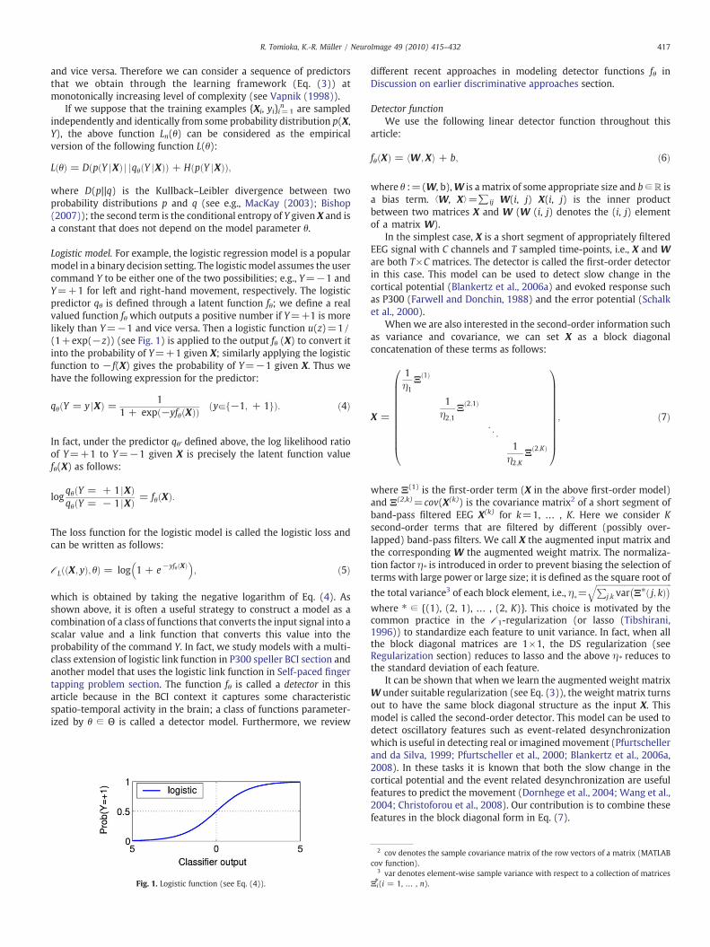
Logistic model. For example, the logistic regression model is a popularmodel in a binary decision setting. The logisticmodel assumes the usercommand Y to be either one of the two possibilities; e.g., Y=−1 andY=+1 for left and right-hand movement, respectively. The logisticpredictor qθ is defined through a latent function fθ; we define a realvalued function fθ which outputs a positive number if Y=+1 is morelikely than Y=−1 and vice versa. Then a logistic function u(z)=1/(1+exp(−z)) (see Fig. 1) is applied to the output fθ (X) to convert itinto the probability of Y=+1 given X; similarly applying the logisticfunction to − f(X) gives the probability of Y=−1 given X. Thus wehave the following expression for the predictor:

qθ Y = y jXð Þ = 11 + exp −yfθ Xð Þð Þ ya −1; + 1f gð Þ: ð4Þ

In fact, under the predictor qθ' defined above, the log likelihood ratioof Y=+1 to Y=−1 given X is precisely the latent function valuefθ(X) as follows:

logqθ Y = + 1 jXð Þqθ Y = − 1 jXð Þ = fθ Xð Þ:

The loss function for the logistic model is called the logistic loss andcan be written as follows:

ℓL X; yð Þ; θð Þ = log 1 + e−yfθ Xð Þ� �; ð5Þ

which is obtained by taking the negative logarithm of Eq. (4). Asshown above, it is often a useful strategy to construct a model as acombination of a class of functions that converts the input signal into ascalar value and a link function that converts this value into theprobability of the command Y. In fact, we study models with a multi-class extension of logistic link function in P300 speller BCI section andanother model that uses the logistic link function in Self-paced fingertapping problem section. The function fθ is called a detector in thisarticle because in the BCI context it captures some characteristicspatio-temporal activity in the brain; a class of functions parameter-ized by θ ∈ Θ is called a detector model. Furthermore, we review

Fig. 1. Logistic function (see Eq. (4)).

different recent approaches in modeling detector functions fθ inDiscussion on earlier discriminative approaches section.

Detector functionWe use the following linear detector function throughout this

article:

fθ Xð Þ = hW ;Xi + b; ð6Þ

where θ :=(W, b),W is a matrix of some appropriate size and b∈R isa bias term. ⟨W, X⟩=∑ij W(i, j) X(i, j) is the inner productbetween two matrices X and W (W (i, j) denotes the (i, j) elementof a matrix W).

In the simplest case, X is a short segment of appropriately filteredEEG signal with C channels and T sampled time-points, i.e., X and Ware both T×C matrices. The detector is called the first-order detectorin this case. This model can be used to detect slow change in thecortical potential (Blankertz et al., 2006a) and evoked response suchas P300 (Farwell and Donchin, 1988) and the error potential (Schalket al., 2000).

When we are also interested in the second-order information suchas variance and covariance, we can set X as a block diagonalconcatenation of these terms as follows:

X =

1η1

Ξ 1ð Þ

1η2;1

Ξ 2;1ð Þ

O1

η2;KΞ 2;Kð Þ

0BBBBBBBBBBB@

1CCCCCCCCCCCA; ð7Þ

where Ξ(1) is the first-order term (X in the above first-order model)and Ξ(2,k)=cov(X(k)) is the covariance matrix2 of a short segment ofband-pass filtered EEG X(k) for k=1, … , K. Here we consider Ksecond-order terms that are filtered by different (possibly over-lapped) band-pass filters. We call X the augmented input matrix andthe corresponding W the augmented weight matrix. The normaliza-tion factor η⁎ is introduced in order to prevent biasing the selection ofterms with large power or large size; it is defined as the square root of

the total variance3 of each block element, i.e., η�=ffiffiffiffiffiffiffiffiffiffiffiffiffiffiffiffiffiffiffiffiffiffiffiffiffiffiffiffiffiffiffiffiffiffiffiffiffiffiP

j;k var Ξ� j; kð Þ� �qwhere ⁎ ∈ {(1), (2, 1), … , (2, K)}. This choice is motivated by thecommon practice in the ℓ1-regularization (or lasso (Tibshirani,1996)) to standardize each feature to unit variance. In fact, when allthe block diagonal matrices are 1×1, the DS regularization (seeRegularization section) reduces to lasso and the above η⁎ reduces tothe standard deviation of each feature.

It can be shown that when we learn the augmented weight matrixW under suitable regularization (see Eq. (3)), the weight matrix turnsout to have the same block diagonal structure as the input X. Thismodel is called the second-order detector. This model can be used todetect oscillatory features such as event-related desynchronizationwhich is useful in detecting real or imaginedmovement (Pfurtschellerand da Silva, 1999; Pfurtscheller et al., 2000; Blankertz et al., 2006a,2008). In these tasks it is known that both the slow change in thecortical potential and the event related desynchronization are usefulfeatures to predict the movement (Dornhege et al., 2004; Wang et al.,2004; Christoforou et al., 2008). Our contribution is to combine thesefeatures in the block diagonal form in Eq. (7).

2 cov denotes the sample covariance matrix of the row vectors of a matrix (MATLABcov function).

3 var denotes element-wise sample variance with respect to a collection of matricesΞi⁎(i = 1, … , n).


RegularizationIn this section we preset three types of regularizers (θ) in our

learning framework (Eq. (3)).The first regularizer is the standard Frobenius norm of the weight

matrix as follows:

VF θð Þ = ‖W‖F =ffiffiffiffiffiffiffiffiffiffiffiffiffiffiffiffiffihW ;Wi

p; ð8Þ

In other words, it is the Euclidean norm of the weight matrix viewedas a vector.

The next three regularizers induce different types of sparsity in theweight matrix. The first two of them are defined as the “linear sum ofgroup-wise norms”, where the group is defined a priori. We assume asimple first-order detector in which the columns correspond toelectrodes and rows correspond to sampled time-points; the tworegularizers are called channel selection regularizer and temporal-basis selection regularizer and are defined as follows:

VC θð Þ =XCc=1

‖W :; cð Þ‖2; ð9Þ

VT θð Þ =XTt=1

‖W t; :ð Þ‖2; ð10Þ

whereW(:, c) denotes the c-th column vector of the weight matrixW,W(t, :) denotes the t-th row vector of W and ||·||2 is the vectorEuclidean norm. In Eq. (9) each row is grouped together. Similarly inEq. (10) each column is grouped together. Thus analogous to ℓ1-regularization (known as lasso (Tibshirani, 1996)) the two regular-izers induce sparsity in the electrode-wise (row-wise), and the time-point-wise (column-wise) manners, respectively. This type of regu-larization is known as group-lasso (Yuan and Lin, 2006) or M-FOCUSS(Cotter et al., 2005) and recently also applied to the reconstruction offocal vector fields (Haufe et al., 2008).

The last regularizer is defined as the linear sum of singular-valuesof the weight matrix W, which is called the dual spectral (DS) norm(Fazel et al., 2001)4.

VDS θð Þ = ‖W‖T :=Xrj=1

σ j Wð Þ; ð11Þ

where σj (W) is the j-th singular value of the weight matrixW and r isthe rank of W. The DS regularization can be considered as anothergeneralization of the ℓ1-regularization; it induces sparsity in thesingular-value spectrum of the weight matrix W. That is, it induceslow-rank matrix W. Similarly to group-lasso, when a singular-component is switched off, all the degrees of freedom associated tothat component (i.e., left and right singular vectors) are simulta-neously switched off. However in contrast to group-lasso regularizer,there is no notion of any group a priori. The DS regularizationautomatically tunes the feature detectors as well as the rank ofW. It isalso interesting to contrast the dual spectral regularizer to theFrobenius norm regularizer (Eq. (8)). The Frobenius norm can berewritten as the ℓ2-norm on the singular-value spectrum as follows:

VF θð Þ =ffiffiffiffiffiffiffiffiffiffiffiffiffiffiffiffiffiffiffiffiffiffiffiTr WhWð Þ

p=

ffiffiffiffiffiffiffiffiffiffiffiffiffiffiffiffiffiffiffiffiffiffiffiffiffiffiffiffiffiffiffiXrj=1

σ2j Wð Þ

q;

ð12Þ

wherewe used the fact that the trace of a positive semidefinitematrix isequal to the sum of its eigenvalues which equals the sum of squaredsingular values of W. Comparing Eq. (12) and Eq. (11), we canunderstand the Frobenius norm and the DS norm as the ℓ2 and ℓ1-norm on the singular-value spectrum of a matrix, respectively. In

4 It is also known as the trace norm (Srebro et al., 2005), the Ky-Fan r-norm (Yuanet al., 2007), and the nuclear norm (Boyd and Vandenberghe, 2004).

machine learning literature, the low-rank enforcing property of thedual spectral norm is well known and has been used in applicationssuch as collaborative filtering (Srebro, 2004; Srebro et al., 2005; Rennieand Srebro, 2005; Abernethy et al., 2006), multi-class classification(Amit et al., 2007), multi-output prediction (Argyriou et al., 2007,2008; Yuan et al., 2007). It has been also successfully applied to theclassification of motor-imagery based BCI (Tomioka and Aihara (2007),see also Discussion on earlier discriminative approaches section).

All the above regularizers give rise to some conic constraints in Eq.(3). The Frobenius and group-lasso-type regularizers (Eqs. (8)–(10))induce the second-order cone constraint and the DS regularizer (Eq.(11)) induces the positive semidefinite cone constraint. In fact,mathematically these cones are understood as generalizations of thepositive-orthant cone induced by the ℓ1- (lasso) regularizer (Farautand Koranyi, 1995). Some algorithmic details of the minimization inEq. (3) are presented in Appendix A.

P300 speller BCI

In this section we apply the general framework presented in Signalanalysis framework section to a brain-controlled spelling systemknown as P300 speller. The design of the spelling system is reviewedin P300 speller system section. The probabilistic predictor modeltailored for the P300 speller system is proposed in Predictor model forP300 speller section. The details about preprocessing can be found inSignal acquisition and preprocessing section.

P300 speller systemHere we briefly describe the P300 speller system designed by

Farwell and Donchin (1988). The subjects are presented a 6×6 tableof 36 letters on the screen (see Fig. 2); they are instructed to focus onthe letter they wish to spell for some specified period for each letter;during that period the rows and columns of the table are intensified(more specifically highlighted) in a random order. It is known that thesubject's brain shows a characteristic reaction with a latency of about300 ms called P300 when the row or column that is intensifiedincludes the letter on which the subject is placing his/her focus. Thusby detecting the P300 response, we can predict the letter that thesubject is trying to spell. Each intensification lasts 100 ms with aninterval of 75 ms afterwards; the intensifications of all 6 rows and 6columns (in a random order) are repeated 15 times; hence one lettertakes 175 ms×12×15=31.5 s. Note that the period of intensification(175 ms) is shorter than the expected reaction of the brain (300 ms).Thus the intervals we analyze are usually overlaps of severalintensifications.

Fig. 2. Table of letters shown on the display in the P300 speller system (Farwell andDonchin, 1988). The third row is intensified.

Fig. 3. Schematic comparison of our trial-wise multinomial detection approach and theconventional epoch-wise binary detection approach. Suppose the alphabetA consists ofthree letters, “a”, “b”, and “c” andwe have three trials containing three epochs each (i.e.,response after the intensification of “a”, “b”, and “c”). The true letter is “c” for all the three


Predictor model for P300 spellerLet the alphabet A be the set of all letters in the table, a trial X be a

list of epochs5 X=(X(1),… , X(12)), X(l) ∈ RT×C be the short segment ofmulti-channel EEG recorded after each intensification (1–6 corre-sponds to columns and 7–12 corresponds to rows), where C is thenumber of channels and T is the number of sampled time-points, andy be the true letter that the subject intends to spell during theintensifications. Inspired by Farwell and Donchin (1988) we modelthe predictive probability over 36 candidate letters proportional tothe exponential of the sum of detector function outputs at the twocorresponding row and column intensifications as follows:

qθ y jXð Þ =exp fθ X col yð Þð Þ

� �m fθ X row yð Þ+6ð Þ� ��

Xy VaA exp fθ X col yVð Þð Þ

� �m fθ X row yVð Þ+6ð Þ� �� ; ð13Þ

where col(y) and row(y) are the indices of the column and the row ofthe letter y on the display (see Fig. 2). It is easy to see that the aboveEq. (13) can be decomposed into a direct product of two six-classmultinomial distribution as follows:

qθ y jXð Þ = efθ X col yð Þð Þð ÞX6l=1

efθ X lð Þð Þ �efθ X row yð Þ+6ð Þð ÞX12

l=7efθ X lð Þð Þ : ð14Þ

Here fθ (X(l)) is a first-order detector that outputs a scalar value foreach intensification as follows:

fθ X lð Þ� �

= hW ;X lð Þi; l = 1; :::;12ð Þ; ð15Þ

where the weight matrix W has T rows and C columns. The bias termis omitted because the probability distribution in Eq. (14) is invariantto a constant shift of Eq. (15). Note that the parameter W is sharedamong all inputs X(l) (l=1, … , 12). Another difference between theproposed predictor model (Eq. (14)) and the general multi-classlikelihood (Bishop, 2007) is that the l-th output value only dependson the l-th input matrix X(l). Furthermore, let a subtrial be thecollection of six epochs within a trial with either row (l=1, … , 6) orcolumn (l=7, … , 12) intensifications; thus a trial consists of twosubtrials. Note that the contribution of the subtrials to the predictor(Eq. (14)) is independent of each other. Thus mathematically Eq. (14)is equivalent to P300 speller for six letters with two times as manytrials. Note that our proposed predictor model (Eq. (13)) can alsoaccommodate novel coding schemes for P300 speller proposed in Hillet al. (2009).

For the decoding, according to Eq. (1), we maximize the posteriorprobability q(y|X) given X with respect to y as follows:

y = argmaxyaA

logqθ y jXð Þ

= argmaxyaA

fθ X col yð Þð Þ� �

m fθ X row yð Þ+6ð Þ� ��

;ð16Þ

which is simply to choose the column and row with maximumresponse.

As we have seen in the previous section, the above model is usedsimultaneously for decoding the letter and learning the parameter W;according to Eq. (2)) the loss function is defined as follows:

ℓ X; yð Þ; θð Þ = − fθ X col yð Þð Þ� �

+ logX6l=1

efθ X lð Þð Þ !

− fθ X row yð Þ+6ð Þ� �

+ logX12l=7

efθ X lð Þð Þ !

:

5 In this section we reserve the term trial for a collection of short segments of EEG(called epoch) recorded after different intensifications for each character.

The above model contrasts sharply to the conventional approach thatfirst trains a binary classifier that detects P300 response and thencombines them to predict the letter (see e.g., Rakotomamonjy andGuigue (2008)) in the following way. The proposed multinomialmodel is normalized in a subtrial-wise manner whereas theconventional binary approach is normalized in an epoch-wisemanner. More specifically, we have a budget of probability one foreach subtrial that we can distribute over the epochs within the sub-trial whereas the conventional binary approach has the same budgetfor each epoch which is distributed between the possibility that itcontains P300 response or not. This epoch-wise normalizationimposes stronger constraint on the detector function than oursubtrial-wise normalization. In fact, the conventional binary approachtries to separate all the positive epochs (which contains P300response) from all the negative epochs (which contains no P300response) whereas the proposed subtrial-wise multinomial approachtries to align the positive epoch in front of the negative epochs in thesame subtrial (see Fig. 3(A)). In other words, only the detector output

trials. Thus “a” and “b” are negative epochs (marked with crosses) and “c” are positiveepochs (marked with circles). (A) Conventional binary model learns strict boundarywhereas the proposed multinomial model only learns alignment. (B) The binarydecision boundary can be nonlinear even when the optimal detector function is linear.

6filtfilt performs zero-phase digital filtering by applying the filter in both the

forward and reverse directions. This is necessary in this dataset because the signal isprovided as a collection of 500ms long segments.


value in a positive epoch relative to the negative epochs in the samesubtrialmatters for the proposed model. Furthermore, even when theoptimal detector function is linear, the binary decision boundary canbe nonlinear as in Fig. 3(B). Moreover there is no class bias problemwhich arise in the conventional binary detection approach becausethe whole (sub)-trial is fed jointly to the predictor. Furthermore wecan directly measure the letter predictor accuracy for model selectionwithout introducing auxiliary performance measure as in Rakotoma-monjy and Guigue (2008).

Signal acquisition and preprocessingWe use the P300 dataset (dataset II) provided by Jonathan R.

Wolpaw, Gerwin Schalk, and Dean Krusienski in the BCI competitionIII (Blankertz et al., 2006b). The dataset includes two subjects namelyA and B. The signal is recorded with a 64 channel EEG amplifier. Welow-pass filter the signal at 20 Hz, down sample the signal to 60 Hz,and cut out an interval of 600ms from the onset of each intensificationas an epoch X(l) ∈ RT×C where T=37 and C=64 (l=1,… , 12). A trialX ∈ (RT×C)12 consists of 12 epochs and is assigned a single letter y ∈A. For each letter, trials (each consisting of 12 epochs) are repeated 15times. These repetitions are simply considered as separate trainingexamples; of course the first trial and the last trial for one letter mighthave different statistical character but the detector would regard thisdifference as inner-class variability and would become invariant aspossible to the difference. Since the training set consists of 85 letters,we have 15·85=1275 training examples consisting of 12 epochs.

Before applying the learning algorithm (Eq. (3)), we applypreprocessing matrices Ps and Pt to the low-pass filtered signal X(l)LP

as X(l)=PtX(l)LP Ps. The spatial and temporal preprocessing matrices Ps

and Pt are defined as follows. For the channel selection regularizer andthe temporal-basis selection regularizer, we choose Ps=diag (σ1

s , … ,σCs)−1 and Pt=diag(σ1

t ,… , σTt)−1 whereσc

s andσtt are the square roots

of the average variance of the c-th channel and the t-th time-point,respectively. This choice approximately normalizes each channel andtime-point to unit variance. However it does notmix different channelsor different time-points because we aim to select a few informativeones from them. For the Frobenius norm and DS norm regularizers, wechosePs=∑s−1/4 andPt=∑t−1/4,where∑s and∑t are thepooledcovariance matrices in the spatial and temporal domain defined asfollows:

Ps =1

12n

Xni=1

X12l=1

cov XLPi lð Þ

� �;

Pt =1

12n

Xni=1

X12l=1

cov XLP⊤

i lð Þ� �

:

The exponent −1/4 is empirically found to produce a signal matrixX(l) that has approximately unit variance for every element. This isbecause the variance of the raw signal is counted both in ∑s and∑t.In contrast to the spatial/temporal selection regularizer, there is noneed to restrict the preprocessing matrices to a diagonal form becausethe goal is to choose a few informative pairs of spatial and temporalfilters.

The test data consists of 100 letters; also 12 different intensifica-tions are repeated 15 times (in a random order) in the test set. Wereport the results of (a) averaging all the 15 repetitions (M=15) and(b) averaging only the first 5 repetitions (M=5) in the prediction ofeach letter.

Self-paced finger tapping problem

In this section, the general framework presented in Signalanalysis framework section is applied to the problem of single-trialprediction of self-paced finger tapping. The problem and the datasetis outlined in Problem setting section. In contrast to the P300 speller

system, because the problem is binary classification, the choice oflink function is rather simple. The challenge is how to incorporatedifferent sources of information, namely the slow change in thecortical potential and the event-related modulation of rhythmicactivity, in a principled manner. To this end, three detector functionsare presented in Preprocessing and predictor model for the self-paced problem section.

Problem settingIn the self-paced finger tapping dataset (dataset IV, BCI competi-

tion 2003 (Blankertz et al., 2004)), the goal is to predict the type ofupcoming voluntary finger movement before it actually occurs(Blankertz et al., 2002). EEG of a subject was recorded while thesubject was typing certain keys on the keyboard at his/her own choiceat the average speed of 1 key stroke per second. The subject usedeither the index finger or the little finger of the left hand or the righthand. Here the task is to predict whether the upcoming key press is bythe left or right hand according to the task at the competition.

Preprocessing and predictor model for the self-paced problemEEG is recorded from 28 electrodes at sampling frequency 1000Hz

and down-sampled to 100 Hz. The raw signal matrix Xraw ∈ RT×C is ashort segment of multi-channel EEG recording starting 630 ms andending 130 ms before each key press, where C=28 and T=50. Thetraining set contains in total 316 trials which consists of 159 left-handand 157 right-hand trials.

Since the problem is binary we use the logistic predictor model(Eq. (4)); thus the decoding is carried out by simply taking the sign ofthe detector function as follows:

y =+ 1 if fθ Xð Þz0;

−1 if fθ Xð Þb0:

(

For the learning of the detector function the logistic loss function(Eq. (5)) is used in Eq. (3).

For the detector function we propose three models. The firstfunction is a simple first-order model that only captures the slowchange in the potential. Thus the weight matrix W in Eq. (6) has Trows and C columns. The input matrix Xraw is low-pass filtered at20 Hz and preprocessed as X=PtXLPPs with Pt=∑t−1/4 andPs=∑s−1/4 as in the P300 speller problem (see Signal acquisitionand preprocessing section in P300 speller BCI section).

The second function consists of both first-order term and a wide-band (7–30 Hz) second-order covariance term which are concate-nated along the diagonal of the input matrix (see Eq. (7)). It is calledthe wide-band second-order model. The first-order term Ξ(1) ispreprocessed in the same way as the above first-order model; thesecond-order term is band-pass filtered at 7–30 Hz and preprocessedwith a spatial whitening matrix ∑s−1/2, i.e., Ξ(2,1)=∑s−1/2cov(XBP)∑s−1/2.

Finally the last function consists of the first-order term and twosecond-order terms that capture the alpha-band (7–15 Hz) and thebeta-band (15–30 Hz) which again form the augmented input matrixby block diagonal concatenation (see Eq. (7)). It is called the double-band second-order model. Similarly, the first-order term Ξ(1) ispreprocessed in the same way as the above models; the twosecond-order terms Ξ(2,1) and Ξ(2,2) are band-pass filtered at 7–15 Hz and 15–30 Hz, respectively, and spatially whitened individually.

All the temporal filtering mentioned above is done using theMATLAB function filtfilt6 because it minimizes the effect of start-up


transients. We test the Frobenius norm regularizer as the base line aswell as the proposed DS norm regularizer. Our aim is to simulta-neously learn and select few informative spatio-temporal filters in asystematic manner.

Results: P300 speller BCI

The result of the proposed framework applied to P300 speller BCI(P300 speller BCI section) is given in this section. Additionallydiscussion including the interpretation provided by the proposedthree sparse regularizers is given in Discussion section.

Fig. 4. Classification accuracy and the number of active components obtained with different r(M=5) and 15 repetitions (M=15), respectively. The dashed lines with error bars show theeach figure: number of active components. The vertical dashed lines show the regularizationThe bottom part shows the number of non-zero singular values of theweight matrix. (B) Channorms. (C) Temporal-basis selection regularizer. The bottom part shows the number of temshows the number of non-zero singular values of the weight matrix.

Performance

Figs. 4 (A–D) show the performance of the proposed decodingmodel with (A) Frobenius norm, (B) channel selection regularizer, (C)temporal-basis selection regularizer, and (D) DS norm regularizer,respectively. The classification accuracy (solid line) obtained at theregularization constant chosen by cross-validation is marked with acircle. The cross-validation accuracy is also shown as dashed lineswith error bars; we show the mean and standard deviation of tworuns of 10-fold cross-validation. Note that we compute the characterrecognition accuracy for each number of repetitions M on the

egularizers. Top part of each figure: the blue and green lines correspond to 5 repetitionscross-validation performance. The solid lines show the test performance. Bottom part ofconstant chosen for the visualization in Figs. 6 and 7. (A) Frobenius norm regularization.nel selection regularizer. The bottom part shows the number of channels with non-zeroporal bases with non-zero norms. (D) Dual spectral norm regularizer. The bottom part

Table 1Classification accuracy in % obtained with four regularizers namely channel selectionregularizer (CSR, Eq. (9)), temporal-basis selection regularizer (TSR, Eq. (10)), and thedual spectral norm regularizer (DS, Eqs. (11)), compared against the winner of thecompetition (R&G).

Subject Frobenius CSR TSR DS R&G

A (M=5) 67 68 64 71 68A (M=15) 98 98 99 99 98B (M=5) 77 81 78 79 76B (M=15) 93 93 95 94 95mean (M=5) 72 74.5 71 75 72mean (M=15) 95.5 95.5 97 96.5 96.5

Fig. 5. The accuracy of the proposed dual spectral regularization compared toRakotomamonjy and Guigue (2008) at variety of number of repetitions.


validation set. Thus we can choose the best model depending on thetarget information transfer rate.

In addition, the number of active components7 is shown at thebottom of each plot. The plot is almost flat for the Frobenius normregularizer, which employs no selection mechanism. The number ofcomponents falls sharply for the channel selection regularizer and thetemporal-basis selection regularizer but it seems that the selectionoccurs at the cost of performance reduction. In contrast, the number ofcomponents (rank) can be greatly reduced with little cost until somepoint for the DS regularization.

Table 1 summarizes the test accuracy obtained at the selectedregularization constant. The result from Rakotomamonjy and Guigue(2008) who won the competition is also shown. Bold and italicnumbers are the best and the second best accuracy for each subjectand number of repetitions. Note that the results of the winner areslightly different from the ones that are available from the official BCIcompetition website; this is because we recomputed the results usingthe scripts provided by the winner8.

Discussion

The performance of the proposed regularizers are comparable tothat of the winner of the competition except for the Frobenius normregularizer. In addition, in Fig. 5, the performance of the proposedmodel with the DS regularizer is compared against that of the winner(R&G) at various number of repetitions M. Although it is difficult todraw any conclusion from such a small test, for both subjects theproposed method is competitive to Rakotomamonjy and Guigue(2008) for most M especially at small number of repetitions. This canbe partly explained by the fact that we choose the regularizationconstant C using the character recognition accuracy on the validationset for each M whereas an auxiliary measure for model selectionbased on the binary classification model is used in Rakotomamonjyand Guigue (2008), which does not take the number of repetitionsinto account.

We should note that although the normalization by ∑t−1/4 and∑s− 1/4 from both sides seems sensible from dimensionalityconsideration and its separability, in principle this should be alsoconsidered as a hyper-parameter that needs to be selected based onthe training data. In fact, we obtained a lower performance bynormalizing each element of the input matrices to unit variance,which is actually not preferable because it cannot be separated intothe spatial part and the temporal part as the above normalization(results not shown).

7 The number of active components is defined as follows: given the weight matrixW let s1, … , sr be the component norms (column-wise norms for the channelselection regularizer, row-wise norms for the temporal-basis selection regularizer andthe singular values for the DS regularizer.) #active components = |sj : sj N 0.01maxj(sj)|.

8 Scripts are available from http://asi.insa-rouen.fr/enseignants/~arakotom/code/bciindex.html.

Different types of sparsity induced by the regularizers are useful inunderstanding how classifiers work and also understanding inter-subject variability. The weight matrices obtained with the threesparsity inducing regularizer are visualized in Figs. 6 and 7 for subjectsA and B, respectively. The first two plots (Figs. 6A, B) and Figs. 7A, B)show the weight matrix including the preprocessing matrices Pt andPs defined as Wraw=PtW Ps which has again T rows and C columns.The upper plot shows the temporal slice of Wraw at the time-pointshown above. The temporal slice Wraw(t, :) is color coded as blue–green–red from negative to positive and since it is a C dimensionalvector, it is mapped on a scalp viewed from above (nose pointingupwards). The lower plot shows the spatial slice Wraw(:, c) for everyelectrode along time. The last plots (Figs. 6C and 7C) show the leadingsingular vectors of the weight matrices obtained with the DSregularization. We first perform singular-value decomposition of thelow-rank weight matrix asW=Udiag(σ1,… , σr)V ⊤ where U is a T× rmatrix and V is a C×r matrix. Then we define a spatial filter wj

s and aspatial pattern ajs as follows:

wsj = PsV :; jð Þ; as

j = Ps� �−1V :; jð Þ j = 1; :::; rð Þ:

A spatial filter is a coefficient vector applied to the raw (low-passfiltered) signal as part of the classifier. On the other hand, the spatialpattern of a given spatial filter is the EEG activity that is optimallycaptured by the corresponding spatial filter. That is ajs is orthogonal toevery wj′

s for j′≠ j. Similarly a temporal filter wjt and a temporal

pattern ajt is defined from U and Pt. Now we have a decomposition ofthe raw coefficient matrix Wraw that includes the preprocessing andclassifier coefficient as Wraw=∑j=1

r σjwjtwj

s. Note that using thespatial/temporal filters we can decompose the first-order model (Eq.(15)) as follows:

fθ X lð Þ� �

= hW ; PtXLPlð ÞP

si =Xrj=1

σ jwt⊤

j XLPlð Þw

sj :

Moreover, one can assume the following generative model for theband-pass filtered signal X(l)

LP:

XLPðlÞ =

Xrj=1

η lð Þj at

jas⊤j + N lð Þ

:

where ajs and ajt functions as a fixed spatial/temporal-basis function,ηj(l) is a task-related component, and N(l) is the non-task-relatedcomponent (i.e., wt⊤

j N lð Þwsj = 0 8jð Þ). Thus the spatial/temporal

http://asi.insa-rouen.fr/enseignants/~arakotom/code/bciindex.html

http://asi.insa-rouen.fr/enseignants/~arakotom/code/bciindex.html

Fig. 6. Spatial/temporal profile of subject A. (A) Channel selection regularizer. ΩC(θ)=57. (B) Temporal-basis selection regularizer. ΩT(θ)=59. (C) Dual spectral regularizer.Ω⁎(θ)=0.70.


patterns aj and filters wj provide forward and backward view on thegeneration of task-related EEG activities, respectively (Parra et al.,2005; Blankertz et al., 2008). Finally, the spatial filter, spatial pattern,and the temporal pattern are plotted from left to right for each left/right singular vector pairs of the leading singular values from top tobottom. The spatial filters/patterns are plotted in the same way asabove. The temporal patterns, which are T dimensional vectors, areplotted along time. The singular value is also shown vertically at theleft end of each row.

The channel selection regularizer (see Figs. 6A and 7A) is good atspatially localizing the discriminative information. For both subjects Aand B we can see occipital focus in the early phase and more parietal-central focus in the later phase.

On the other hand, the temporal-basis selection regularizerlocalizes the discriminative information in the temporal domain. Forsubject A (Fig. 6B bottom), there is a prominent negative peak at183 ms and a broad positive component from 350 ms to 500 ms,which roughly agree with the early occipital component and the late

Fig. 7. Spatial/temporal profile of subject B. (A) Channel selection regularizer. ΩC(θ)=66. (B) Temporal-basis selection regularizer. ΩT(θ)=51. (C) Dual spectral regularizer.Ω⁎(θ)=0.89.


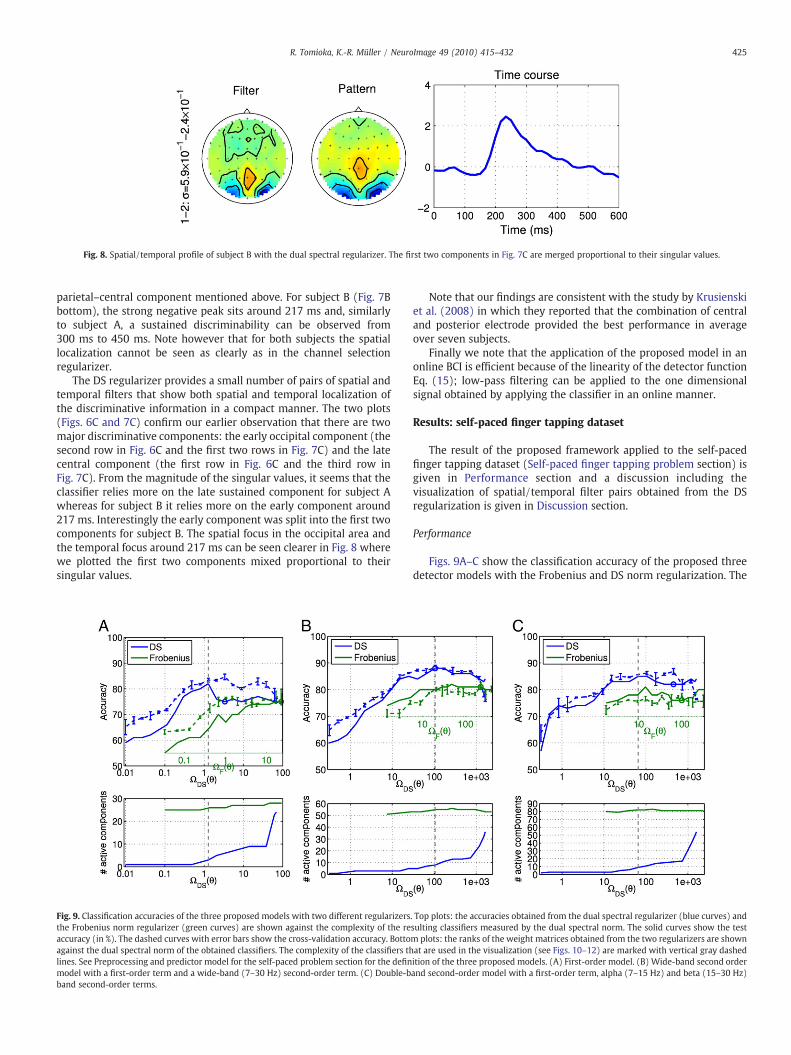
Fig. 8. Spatial/temporal profile of subject B with the dual spectral regularizer. The first two components in Fig. 7C are merged proportional to their singular values.


parietal–central component mentioned above. For subject B (Fig. 7Bbottom), the strong negative peak sits around 217 ms and, similarlyto subject A, a sustained discriminability can be observed from300 ms to 450 ms. Note however that for both subjects the spatiallocalization cannot be seen as clearly as in the channel selectionregularizer.

The DS regularizer provides a small number of pairs of spatial andtemporal filters that show both spatial and temporal localization ofthe discriminative information in a compact manner. The two plots(Figs. 6C and 7C) confirm our earlier observation that there are twomajor discriminative components: the early occipital component (thesecond row in Fig. 6C and the first two rows in Fig. 7C) and the latecentral component (the first row in Fig. 6C and the third row inFig. 7C). From the magnitude of the singular values, it seems that theclassifier relies more on the late sustained component for subject Awhereas for subject B it relies more on the early component around217 ms. Interestingly the early component was split into the first twocomponents for subject B. The spatial focus in the occipital area andthe temporal focus around 217 ms can be seen clearer in Fig. 8 wherewe plotted the first two components mixed proportional to theirsingular values.

Fig. 9. Classification accuracies of the three proposed models with two different regularizersthe Frobenius norm regularizer (green curves) are shown against the complexity of the reaccuracy (in %). The dashed curves with error bars show the cross-validation accuracy. Bottoagainst the dual spectral norm of the obtained classifiers. The complexity of the classifiers thlines. See Preprocessing and predictor model for the self-paced problem section for the definmodel with a first-order term and a wide-band (7–30 Hz) second-order term. (C) Double-bband second-order terms.

Note that our findings are consistent with the study by Krusienskiet al. (2008) in which they reported that the combination of centraland posterior electrode provided the best performance in averageover seven subjects.

Finally we note that the application of the proposed model in anonline BCI is efficient because of the linearity of the detector functionEq. (15); low-pass filtering can be applied to the one dimensionalsignal obtained by applying the classifier in an online manner.

Results: self-paced finger tapping dataset

The result of the proposed framework applied to the self-pacedfinger tapping dataset (Self-paced finger tapping problem section) isgiven in Performance section and a discussion including thevisualization of spatial/temporal filter pairs obtained from the DSregularization is given in Discussion section.

Performance

Figs. 9A–C show the classification accuracy of the proposed threedetector models with the Frobenius and DS norm regularization. The

. Top plots: the accuracies obtained from the dual spectral regularizer (blue curves) andsulting classifiers measured by the dual spectral norm. The solid curves show the testm plots: the ranks of the weight matrices obtained from the two regularizers are shownat are used in the visualization (see Figs. 10–12) are marked with vertical gray dashedition of the three proposed models. (A) First-order model. (B) Wide-band second orderand second-order model with a first-order term, alpha (7–15 Hz) and beta (15–30 Hz)

Table 2Comparison of the complexity (in terms of the number of parameters) and the performance of three proposed models and two earlier studies.

First-ordermodel

Wide-band (7–30 Hz)second-order model

Double-band(7–15 Hz; 15–30 Hz)second-order model

Wang et al. (2004)(1st-order +wide-band(10–33 Hz) +19 selected channels)

SOBDA(1st-order +wide-band(10–33 Hz))

#parameters 1401 (433) 1807 (341) 2213 (559) 282 135DS 75 (85) 88 (88) 82 (87) 84 87Frobenius 75 (77) 81 (81) 76 (78)

In the first row the number of parameters is shown (see main text for the derivation); the number of active parameters is also shown in parenthesis for the proposed models. Theclassification accuracy is shown in %. For the proposed models the accuracy obtained with two regularization strategies are shown. The cross-validation accuracy used for theselection of the regularization constant is shown inside parentheses.

9 The number of active parameters is calculated from the rank of the weight matrix,i.e., rank = r matrix of size R × C has (R + C)r − r2 active parameters.10 Since the block weight matrix associate to the second-order component (see Eq.(7)) is symmetric, we show the eigenvalues instead of singular values for the second-order components.


2×10 fold cross-validation accuracy used for the selection of theregularization constant is also shown as a dashed curve with errorbars for each detector model and regularizer. The accuracies obtainedat the selected regularization constants are marked with circles. Theaccuracy is plotted at the complexity measured by the DS norm for theclassifiers obtained with the two regularizers. This is done in order tocompare the performance of the two classifiers at the samecomplexity. The original complexity measure of the Frobenius normregularized classifiers is also shown as second axis in each figure. Notethat this is only possible when the DS norm of the Frobeniusregularized model grows monotonically with the regularizationconstant.

The performance obtained with the two regularizers is summa-rized in Table 2. The performance of the winner of the competition(Wang et al., 2004) and a recently proposed bilinear discriminantanalysis (Christoforou et al., 2008) is also shown. The best accuracy88% is obtained with the wide-band second-order model with the DSregularization which also achieved the highest with respect to thecross-validation accuracy.

Discussion

In Fig. 9A we can see that the performance of the DS normregularizer is higher than the Frobenius norm regularizer over thewhole range of complexity. The performance of the two regularizersconverges to the same value when the highest complexity is allowed.Indeed the training loss Ln(θ) is less than 10−10 at the highestcomplexity. Thus the difference in the regularizer plays almost norole. Similar trends can also be seen in Figs. 9B and 9C.

Incorporating the wide-band (7–30 Hz) second-order termsignificantly improves the performance (see Fig. 9B) as reportedearlier in (Dornhege et al., 2004; Wang et al., 2004; Christoforou et al.,2008). However the performance is reduced if we allow furtherflexibility by dealing with the alpha-band (7–15 Hz) and beta-band(15–30 Hz) separately (see Fig. 9C). One possible explanation is over-fitting. In addition, the cross-validation failed to predict the drop inthe accuracy aboveΩDS(θ)N100. Strong correlation between the alphaand beta-band may also account for the poor performance; i.e.,dealing with the two bands separately may not provide moreinformation in comparison to the increased dimensionality.

In addition, the dimensionalities of the proposed detector modelsare compared to those of the two earlier studies in Table 2. Thenumber of parameters is calculated as follows: for the first-ordermodel it is 28(channels)×50(time-points) 1(bias)=1401; for thesecond-order model adding 406 (the degree of freedom of 28×28symmetric matrix) it is 1807; for the double-band second-ordermodel it is 2213 with an additional 406. For Wang et al. (2004),since they used a rank=2 first-order term with 4 time-points((28+4)·2=64), a rank=6 wide-band second-order term with 4time-points ((28+4)·6=192), hand-chosen 19 electrodes with afixed temporal filter (19), and 3 classifier weights and 4 biasterms, it is 282. For SOBDA (Christoforou et al., 2008), since theyused a rank=1 first-order term with 50 time-points and a

rank=2 second-order term with no temporal information, and asingle bias term, it is 28+50+28·2+1=135. Although, the rawdimensionality of the proposed models are higher than those ofthe two earlier studies, the numbers of active parameters9 at theselected regularization constant (shown inside the parentheses)are of the same order as the earlier studies. Importantly for theproposed models, the rank is automatically tuned through theregularization. Similar models which in contrast had to fix the ranka priori have been employed in earlier studies (see Wang et al.(2004); Christoforou et al. (2008) and Discussion on earlierdiscriminative approaches section).

The spatial/temporal profiles of the three proposed models arevisualized in Figs. 10–12. See Discussion section in Results: P300speller BCI section for the definition of spatial/temporal filters andpatterns. The top two components obtained from the first-orderterm seems to be preserved from the simple first-order model to themost complex double-band second-order model. The first compo-nent clearly focuses on the lateralized readiness potential. This canbe seen from the bipolar structure of the spatial pattern (two peakswith opposite signs on left and right motor cortices) as well as thetemporal profile that drops monotonically towards the key press.The meaning of the second component is not obvious. From thedownward trend along time, we conjecture that it also detects somepart of the readiness potential that is not captured by the firstcomponent though the contribution of this component to theclassifier is one order smaller than the first component.

In Fig. 11, we can find typical spatial patterns for event-related (de)-synchronization (ERD/ERS (Pfurtscheller and da Silva,1999). The first second-order component (third row) capturesERD in the right-hand area (which can be seen from the negativesign of the eigenvalue10 shown next to the filter) and the secondsecond-order component (forth row) captures ERD in the left-hand area.

Interestingly this discriminability is mainly due to the beta-band.In Fig. 12, we can find spatial filter/pattern pairs that look similar tothe ERD/ERS components in Fig. 11 in the bottom two rows(components obtained from the beta-band) though the order isreversed. Then what are the two alpha components (rows 3–4)doing? From the spatial filters they might seem to be focusing on theright motor cortex which delivers the ERD in the left-hand trials.However the negative signs of the eigenvalues and the spatialpatterns suggest that these components detect ERD in the right-hand trials. We confirm this in Fig. 13 where we plot the log powers ofthe spatially filtered beta-band features against those of alpha-bandfeatures. Indeed both alpha-band features show lower magnitude inthe right-hand trials than in the left-hand trials.

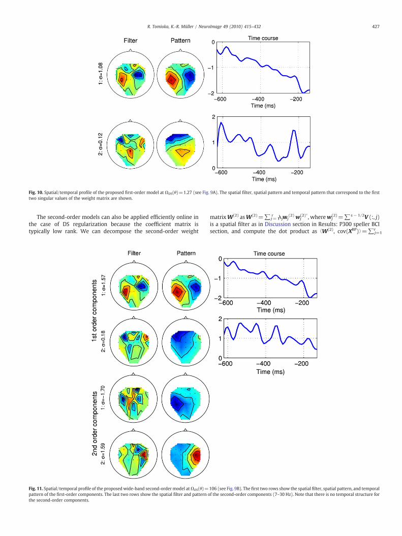
Fig. 10. Spatial/temporal profile of the proposed first-order model at ΩDS(θ)=1.27 (see Fig. 9A). The spatial filter, spatial pattern and temporal pattern that correspond to the firsttwo singular values of the weight matrix are shown.


The second-order models can also be applied efficiently online inthe case of DS regularization because the coefficient matrix istypically low rank. We can decompose the second-order weight

Fig. 11. Spatial/temporal profile of the proposed wide-band second-order model atΩDS(θ)=pattern of the first-order components. The last two rows show the spatial filter and pattern othe second-order components.

matrixW(2) asW(2)=∑j=1r λjwj

(2)wj(2)⊤, wherewj

(2)=∑s−1/2V (:, j)is a spatial filter as in Discussion section in Results: P300 speller BCIsection, and compute the dot product as ⟨W(2), cov(XBP)⟩=∑j=1

r

106 (see Fig. 9B). The first two rows show the spatial filter, spatial pattern, and temporalf the second-order components (7–30 Hz). Note that there is no temporal structure for

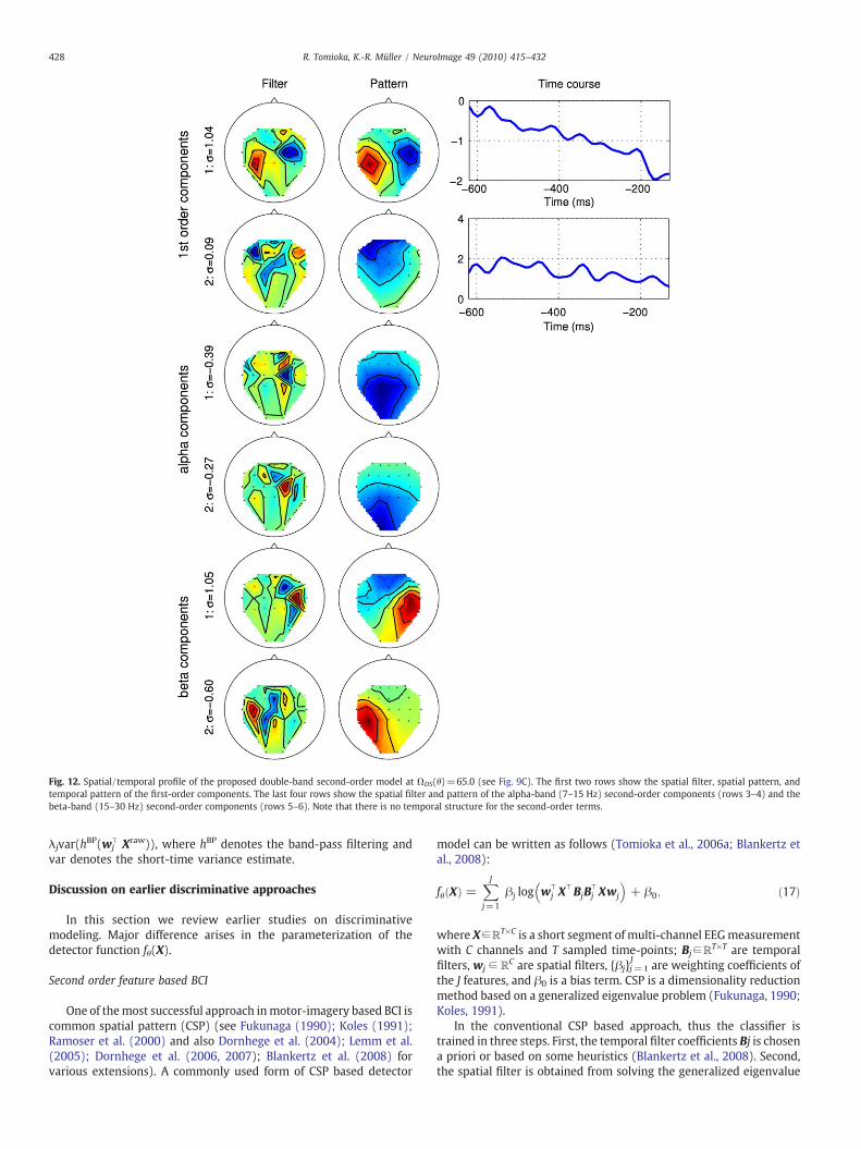
Fig. 12. Spatial/temporal profile of the proposed double-band second-order model at ΩDS(θ)=65.0 (see Fig. 9C). The first two rows show the spatial filter, spatial pattern, andtemporal pattern of the first-order components. The last four rows show the spatial filter and pattern of the alpha-band (7–15 Hz) second-order components (rows 3–4) and thebeta-band (15–30 Hz) second-order components (rows 5–6). Note that there is no temporal structure for the second-order terms.


λjvar(hBP(wj⊤ Xraw)), where hBP denotes the band-pass filtering and

var denotes the short-time variance estimate.

Discussion on earlier discriminative approaches

In this section we review earlier studies on discriminativemodeling. Major difference arises in the parameterization of thedetector function fθ(X).

Second order feature based BCI

One of themost successful approach inmotor-imagery based BCI iscommon spatial pattern (CSP) (see Fukunaga (1990); Koles (1991);Ramoser et al. (2000) and also Dornhege et al. (2004); Lemm et al.(2005); Dornhege et al. (2006, 2007); Blankertz et al. (2008) forvarious extensions). A commonly used form of CSP based detector

model can be written as follows (Tomioka et al., 2006a; Blankertz etal., 2008):

fθ Xð Þ =XJj=1

βj log wh

j XhBjB

h

j Xwj

� �+ β0; ð17Þ

where X∈RT×C is a short segment of multi-channel EEGmeasurementwith C channels and T sampled time-points; Bj∈RT×T are temporalfilters, wj ∈ RC are spatial filters, {βj}j=1

Jare weighting coefficients of

the J features, and β0 is a bias term. CSP is a dimensionality reductionmethod based on a generalized eigenvalue problem (Fukunaga, 1990;Koles, 1991).

In the conventional CSP based approach, thus the classifier istrained in three steps. First, the temporal filter coefficients Bj is chosena priori or based on some heuristics (Blankertz et al., 2008). Second,the spatial filter is obtained from solving the generalized eigenvalue

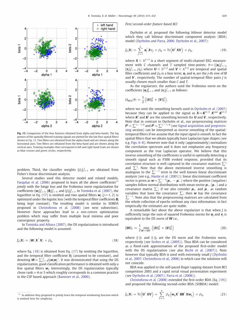
Fig. 13. Comparison of the four features obtained from alpha and beta-bands. The logpowers of the spatially filtered training signals are plotted for the last four spatial filtersshown in Fig. 12. Two filters are obtained from the alpha-band and are shown along thehorizontal axes. Two filters are obtained from the beta-band and are shown along thevertical axes. Training examples that correspond to left and right hand trials are shownas blue crosses and green circles, respectively.


problem. Third, the classifier weights {βj}j=1J are obtained from

Fisher's linear discriminant analysis.Several studies used this detector model and related models.

Farquhar et al. (2006) proposed to learn all the above coefficients11

jointly with the hinge loss and the Frobenius norm regularization forcoefficients {wj}j=1

J , {Bj}j=1J , and {βj}j=1

J . In Tomioka et al. (2007), thelogarithm in Eq. (17) is omitted and two spatial filters wj (j=1, 2) isoptimized under the logistic loss (with the temporal filter coefficients Bj

being kept constant). The resulting model is similar to SOBDAproposed in Christoforou et al. (2008) (see next subsection).However these approaches lead to a non-convex optimizationproblem which may suffer from multiple local minima and poorconvergence property.

In Tomioka and Aihara (2007), the DS regularization is introducedand the following model is assumed:

fθ Xð Þ = hW ;XhXi + β0; ð18Þ

where Eq. (18) is obtained from Eq. (17) by omitting the logarithm,and the temporal filter coefficient Bj (assumed to be constant), anddenoting W=∑j=1

J βjwjwj⊤. It was demonstrated that using the DS

regularization, good classification performance is obtainedwith only afew spatial filters wj. Interestingly, the DS regularization typicallychose rank=4 or 5 which roughly corresponds to a common practicein the CSP based approach (Ramoser et al., 2000).

11 In addition they proposed to jointly learn the temporal windowing function whichis omitted here for simplicity.

First/second-order feature based BCI

Dyrholm et al. proposed the following bilinear detector modelwhich they call bilinear discriminant component analysis (BDA)model (Dyrholm and Parra, 2006; Dyrholm et al., 2007):

fθ Xð Þ =XJj=1

uh

j Xυj + β0 = Tr UhXV� �

+ β0; ð19Þ

where X ∈ RC×T is a short segment of multi-channel EEG measure-ment with C channels and T sampled time-points; θ=({uj}j=1

J ,{vj}j=1

J , β0) where U ∈ RC×J and V ∈ RT×J are temporal and spatialfilter coefficients and β0 is a bias term; uj and vj are the j-th row of Uand V , respectively. The number of spatial-temporal filter pairs J isusually chosen much smaller than C and T.

As the regularizer, the authors used the Frobenius norm on thecoefficients {uj}j=1

J and {vj}j=1J as follows:

VBDA θð Þ = 12

‖U‖2F + ‖V‖

2F

� �;

where we omit the smoothing kernels used in Dyrholm et al. (2007)because they can be applied to the signal as X=Kt1/2 Xraw Ks1/2

where Kt and Ks are the smoothing kernels for U and V , respectively.Note that in contrast to Dyrholm et al., our preprocessing matricesPs=∑s−1/4 and Pt=∑t−1/4 (see Signal acquisition and preproces-sing section) can be interpreted as inverse smoothing of the spatial/temporal filters if we assume that the input signal is smooth. In fact thespatial filters that we obtain typically have Laplacian type shapes (seee.g. Figs. 6–8). However note that it only (approximately) normalizesthe correlation spectrum and it does not emphasize any frequencycomponent as the true Laplacian operator. We believe that thisinverse smoothing of the coefficients is useful in optimally detecting asmooth signal such as P300 evoked response, provided that itscorrelation structure is well captured in the covariance matrices ∑s

and ∑t. Note that the above mentioned inverse smoothing isanalogous to the ∑−1 term in the well known linear discriminantanalysis (see e.g., Hastie et al. (2001)); linear discriminant coefficientvector is given as w=∑−1(μ+ − μ−) where the positive (negative)samples follow normal distributions with mean vector μ+ (μ−) and acovariance matrix ∑; if we also consider μ+ and μ− as randomvariables that have the covariance ∑, then w has the covariance∑−1. Note also that the preprocessing matrices are calculated fromthe whole collection of epochs without any class information; in factempirically the estimates are quite stable.

A remarkable fact about the above regularizer is that when J issufficiently large the sum of squared Frobenius norms for uj and vj isequivalent to the DS norm of W i.e.,

‖W‖T =12

minW=UVh

‖U‖2F + ‖V‖

2F

� �ð20Þ

where ‖·‖⁎ and ‖·‖F are the DS norm and the Frobenius norm,respectively (see Srebro et al. (2005)). Thus BDA can be consideredas a fixed-rank approximation of the proposed first-order modelwith the DS regularization (see also Recht et al. (2007)). Notehowever that typically BDA is used with extremely small J (Dyrholmet al., 2007; Christoforou et al., 2008) in which case the solutions willnot coincide.

BDA was applied to the self-paced finger tapping dataset from BCIcompetition 2003 and a rapid serial visual presentation experiment(see Dyrholm et al. (2007); Parra et al. (2008)).

Christoforou et al. (2008) extended the first-order BDA (Eq. (19))and proposed the following second-order BDA (SOBDA) model:

fθ Xð Þ = Tr UhXV� �

+XKk=1

βk wkXhBBhXwk

� �+ β0; ð21Þ


where U ∈ RC×J and V ∈ RT×J are the first-order temporal and spatialfilter coefficients as in Eq. (19) and w ∈ RC and B ∈ RT×T are thesecond-order spatial and temporal filter coefficients. They directlyoptimized all the coefficients U, V , wk and B with the logistic lossfunction and squared Frobenius norm penalty on the coefficients. Wecan see that when the temporal filter matrix B is kept constant, Eq.(21) can be written in the form of Eq. (6) by using the block diagonalconcatenation (Eq. (7)).

Conclusion

In this article we have proposed a novel unified framework forsignal analysis in EEG-based BCI. The proposed framework focuses onprobabilistic predictors from which the decoding and learningalgorithms are naturally deduced. The proposed framework includesconventional binary single-trial EEG classification as a special case butit is oriented to the final goal in BCI i.e., to predict the intention of auser in contrast to the training of a binary classifier as an intermediatestep. This is very much in the spirit of Vapnik (1998): solving theproblem directly instead of an indirect multi-step procedure.Moreover, the issues of feature learning, feature selection, and featurecombination are addressed through regularization. This allows us toperform feature learning jointly with the training of the predictormodel in a convex optimization framework. Note that although theproposed training procedure (Discriminative learning section) mightseem exotic to some EEG practitioners, the resulting detector functionis linear and the decoding procedures (see e.g., Eq. (16)) have theintuitive forms as in the previous studies (Farwell and Donchin, 1988;Krusienski et al., 2008).

In the P300 speller problem we have demonstrated how thelearning algorithm derived from a natural predictor model can bedifferent from the conventionally used binary classification approach.In fact, we have shown that the epoch-wise normalization imposed bythe conventional approach may make it difficult to find a simpledetector function. Furthermore different regularizers have revealeddifferent aspects of the localization of the discriminative information.The spatial localization was investigated through the channelselection regularizer. Although the number of electrodes did notsignificantly reduce without compromising the performance, theplots have shown strong focus on occipital to central area. The lowperformance of the strongly regularized models may be attributed tovolume conduction effects. Even if the source activities are spatiallylocalized, volume conduction spreads them over a wide area, makingit difficult to recover the activity from a small number of electrodes.The temporal localization was similarly investigated through thetemporal-basis selection regularizer. Interestingly the temporalprofiles have shown stronger inter-subject variability than thespatial profile. The dual spectral regularization has revealed bothspatial and temporal profiles in a compact manner. All threeregularizers performed comparable to the winner of the BCIcompetition while the dual spectral regularizer being competitive.However from the point of view of understanding the classifier, thethree regularizers provided complimentary views that made itpossible to find a consistent neurophysiological interpretation foreach subject. The use of, say, the channel selection regularizer alonewould not have allowed us to gain such insights. It is also importantto mention that the complimentary views were particularly usefulin deciding the complexity in plot Figs. 6 and 7. Stronglyregularized predictors tend to be over-simplified and the plots donot account for the success at the more complex predictors selectedby the cross-validation. On the other hand, the predictor at thecomplexity selected by the cross-validation did not always providethe best intuition.

In the self-paced finger tapping problem we have addressed theissue of how to learn, select, and combine features from differentsources. We have employed the DS regularization on the augmented

weight matrix. The input feature matrices were concatenated alongthe diagonal to form an augmented input feature matrix. The low-rank factorized predictor obtained from the DS regularization alwaysoutperformed the naive Frobenius norm regularization. Moreover, theproposedmodel has shown the highest performance in comparison tothe winner of the BCI competition as well as the recently proposedsecond-order bilinear discriminant model.

Recent discriminative approaches are also discussed and theconnection between our DS regularization and the sum-of-squared-Euclidean-norms regularization with fixed number of componentsused in (Dyrholm et al., 2007; Tomioka et al., 2007; Christoforou et al.,2008) is also pointed out. However often these models are used withonly an extremely small number of components in which case theabove equivalence does not hold.

The key idea in our approach is to focus on directly predicting theintention of a user. This enabled us to approach decoding and learningin a unified and systematic manner and to avoid intermediate steps.Note that this idea applies not only to other BCI paradigms includinginvasive BCIs but also to general discriminative neurophysiologicalparadigms even beyond EEG.

Furthermore we have shown that our discriminative approach canbe considered as a novel visualization technique of the brain activityof a subject during tasks since it focuses on the basic components thatare useful in predicting the intention of the subject. It reveals themostrelevant piece of discriminant information in the subject's brainactivity. Other types of decomposition problems such as multi-waytensor factorization (Harshman, 1970; Mørup et al., 2008)may also betackled in a similar manner from the discriminative point of viewconsidered in this work.

Acknowledgments

This work was supported in part by grants of Japan Society for thePromotion of Science (JSPS) through the Global COE program(Computationism as a Foundation for the Sciences), Bundesminister-ium für Bildung und Forschung (BMBF), FKZ 01IB001A (brainwork),01GQ0850 (BFNT) and 01GQ0415 (BCCNB), Deutsche Forschungsge-meinschaft (DFG), MU 987/3-1 (Vital-BCI), the FP7-ICT Programme ofthe European Community, under the PASCAL2 Network of Excellence,ICT-216886 and project ICT-2008-224631 (TOBI). This publicationonly reflects the authors' views. We thank Benjamin Blankertz, StefanHaufe, Kazuyuki Aihara, Motoaki Kawanabe, Masashi Sugiyama, DavidWipf, Srikantan Nagarajan, and Hagai Attias for valuable discussions.Part of this work was done while the authors stayed at FraunhoferFIRST.

Appendix A. Details of the algorithm

We used the projected gradient method described in Kim et al.(2006); Tomioka and Sugiyama (2008) for the optimization of Eq.(3) with the DS regularizer (Eq. (11)). The efficiency of the projectedgradient method varies depending on the regularization constant C;it is faster for strong regularization (small C) and slower for weakregularization (large C.) For the P300 problem in Results: P300speller BCI section, it takes about 5–6 min to obtain the solution for asingle regularization constant around the best value C ≃ 5 on aworkstation with two 3.3 GHz dual core Xeon processors and 8GB ofRAM.

The channel selection regularizer and the temporal-basis selectionregularizer (Eqs. (9) and (10)) are rewritten into the following linearpenalty formulation:

minimizeθ

Ln θð Þ + λV θð Þ; ð22Þ

and the steepest descent subgradient method described in Andrewand Gao (2007) (see also Yu et al. (2008)) was used for the


optimization with 20 log-linearly spaced candidates of λ from theinterval [0.01, 100]. The above formulation is equivalent to Eq. (3) inthe sense that for any regularization constant C if the solution ofEq. (3) is unique, then there is a λ N 0 in Eq. (22) that yields the samesolution with Ω(θ)=C; conversely for any λN0, Eq. (3) withC=Ω(θ⁎) gives the same solution, where θ⁎ is the solution of Eq.(22) for the given λ.

For the Frobenius norm regularizer (Eq. (8)), we rewrite Eq. (3)into the following squared penalty formulation:

minimizeθ

Ln θð Þ + λ‖W‖2F ;

and the limited memory BFGS method (Nocedal and Wright, 1999)was used. The above squared norm formulation is again equivalent toEq. (3).

We have recently been developing a new optimization algorithmfor all the sparse regularizers in the linear penalty formulation (Eq.(22)) (Tomioka and Sugiyama, in press). The code is also availablefrom http://www.ibis.t.u-tokyo.ac.jp/ryotat/dal/. However the newalgorithm is still an early release still to be improved; note that thisnovel optimizer was not used for the computation of the results in thispaper.

References

Abernethy, J., Bach, F., Evgeniou, T., Vert, J.-P., September 2006. Low-rank matrixfactorization with attributes. Tech. Rep. N-24/06/MM, Ecole des mines de Paris,France.

Amit, Y., Fink, M., Srebro, N., Ullman, S., 2007. Uncovering shared structures inmulticlass classification. ICML '07: Proceedings of the 24th International Confer-ence on Machine learning. ACM Press, New York, NY, USA, pp. 17–24.

Andrew, G., Gao, J., 2007. Scalable training of L1-regularized log-linear models. Proc. ofthe 24th International Conference on Machine learning. ACM, New York, NY, USA,pp. 33–40.

Argyriou, A., Evgeniou, T., Pontil, M., 2007. Multi-task feature learning. In: Schölkopf, B.,Platt, J., Hoffman, T. (Eds.), Advances in Neural Information Processing Systems 19.MIT Press, Cambridge, MA, pp. 41–48.

Argyriou, A., Micchelli, C.A., Pontil, M., Ying, Y., 2008. A spectral regularizationframework for multi-task structure learning. In: Platt, J., Koller, D., Singer, Y.,Roweis, S. (Eds.), Advances in Neural Information Processing Systems 20. MIT Press,Cambridge, MA, pp. 25–32.

Birbaumer, N., Ghanayim, N., Hinterberger, T., Iversen, I., Kotchoubey, B., Kübler, A.,Perelmouter, J., Taub, E., Flor, H., 1999. A spelling device for the paralysed. Nature398, 297–298.

Bishop, C.M., 2007. Pattern Recognition and Machine Learning. Springer.Blankertz, B., Curio, G., Müller, K.-R., 2002. Classifying single trial EEG: Towards brain

computer interfacing. In: Diettrich, T.G., Becker, S., Ghahramani, Z. (Eds.), Advancesin Neural Inf. Proc. Systems (NIPS 01), Vol. 14, pp. 157–164.

Blankertz, B., Müller, K.-R., Curio, G., Vaughan, T.M., Schalk, G., Wolpaw, J.R.,Schlögl, A., Neuper, C., Pfurtscheller, G., Hinterberger, T., Schröder, M.,Birbaumer, N., 2004. The BCI competition 2003: Progress and perspectives indetection and discrimination of EEG single trials. IEEE Trans. Biomed. Eng. 51(6), 1044–1051.

Blankertz, B., Dornhege, G., Krauledat, M., Müller, K.R., Kunzmann, V., Losch, F., Curio, G.,2006a. The Berlin brain–computer interface: EEG-based communication withoutsubject training. IEEE Trans. Neural Sys. Rehab. Eng. 14 (2), 147–152.

Blankertz, B., Müller, K.-R., Krusienski, D., Schalk, G., Wolpaw, J.R., Schlögl, A.,Pfurtscheller, G., Millán, J. del R., Schröder, M., Birbaumer, N., 2006b. The BCIcompetition III: Validating alternative approaches to actual BCI problems. IEEETrans. Neural Sys. Rehab. Eng. 14 (2), 153–159 see also the webpage: http://www.bbci.de/competition/iii/.

Blankertz, B., Dornhege, G., Krauledat, M., Müller, K.-R., Curio, G., 2007. The non-invasive Berlin brain-computer interface: fast acquisition of effective performancein untrained subjects. NeuroImage 37 (2), 539–550.

Blankertz, B., Tomioka, R., Lemm, S., Kawanabe, M., Müller, K.-R., 2008. Optimizingspatial filters for robust EEG single-trial analysis. IEEE Signal Proc. Magazine 25 (1),41–56.

Boyd, S., Vandenberghe, L., 2004. Convex Optimization. Cambridge University Press.Christoforou, C., Sajda, P., Parra, L.C., 2008. Second order bilinear discriminant analysis

for single trial EEG analysis. In: Platt, J., Koller, D., Singer, Y., Roweis, S. (Eds.),Advances in Neural Information Processing Systems 20. MIT Press, Cambridge, MA,pp. 313–320.

Cotter, S.F., Rao, B.D., Engan, K., Kreutz-Delgado, K., 2005. Sparse solutions to linearinverse problems with multiple measurement vectors. IEEE Trans. Signal Process53 (7), 2477–2488.

Curran, E.A., Stokes, M.J., 2003. Learning to control brain activity: a review of theproduction and control of EEG components for driving brain–computer interface(BCI) systems. Brain Cogn. 51, 326–336.

Dornhege, G., Blankertz, B., Curio, G., Müller, K.-R., Jun. 2004. Boosting bit rates in non-invasive EEG single-trial classifications by feature combination and multi-classparadigms. IEEE Trans. Biomed. Eng. 51 (6), 993–1002.

Dornhege, G., Blankertz, B., Krauledat, M., Losch, F., Curio, G., Müller, K.-R., 2006.Combined optimization of spatial and temporal filters for improving brain–computer interfacing. IEEE Trans. Biomed. Eng. 53 (11), 2274–2281.

Dornhege, G., Millán, J. del R., Hinterberger, T., McFarland, D., Müller, K.-R. (Eds.), 2007.Towards Brain-Computer Interfacing. MIT Press.

Dyrholm, M., Parra, L.C., 2006. Smooth bilinear classification of EEG. In: Proceedings ofthe IEEE 2006 International Conference of the Engineering in Medicine and BiologySociety.

Dyrholm, M., Christoforou, C., Parra, L.C., 2007. Bilinear discriminant componentanalysis. J. Mach. Learn. Res. 8, 1097–1111.

Faraut, J., Koranyi, A., 1995. Analysis on Symmetric Cones. Oxford University Press.Farquhar, J., Hill, J., Schölkopf, B., 2006. Learning optimal EEG features across time,

frequency and space. In NIPS 2006 workshop Current Trends in Brain-ComputerInterfacing.

Farwell, L., Donchin, E., 1988. Talking off the top of your head: toward a mentalprosthesis utilizing event-related brain potentials. Electroencephalogr. Clin.Neurophysiol. 70 (6), 510–523.

Fazel, M., Hindi, H., Boyd, S.P., 2001. A Rank minimization heuristic with application tominimum order system approximation. In: Proceedings of the American ControlConference.

Fukunaga, K., 1990. Introduction to Statistical Pattern Recognition, 2nd Edition.Academic Press, Boston.

Harshman, R., 1970. Foundations of the PARAFAC procedure: models and conditions foran “explanatory” multi-modal factor analysis. UCLA Work. Pap. Phon. 16, 1–84.

Hastie, T., Tibshirani, R., Friedman, J., 2001. The Elements of Statistical Learning.Springer, Verlag.

Haufe, S., Nikulin, V.V., Ziehe, A., Müller, K.-R., Nolte, G., 2008. Combining sparsity androtational invariance in EEG/MEG source reconstruction. NeuroImage 42 (2), 726–738.

Haynes, J.D., Rees, G., 2006. Decoding mental states from brain activity in humans. Nat.Rev. Neurosci. 7 (7), 523–534.

Hill, J., Farquhar, J., Martens, S., Bieβmann, F., Schölkopf, B., 2009. Effects of stimulustype and of errorcorrecting code design on bci speller performance. In: Koller, D.,Schuurmans, D., Bengio, Y., Bottou, L. (Eds.), Advances in Neural InformationProcessing Systems 21. MIT Press, Cambridge, MA, pp. 665–672.

Hochberg, L.R., Serruya, M.D., Friehs, G.M., Mukand, J.A., Saleh, M., Caplan, A.H., Branner,A., Chen, D., Penn, R.D., Donoghue, J.P., 2006. Neuronal ensemble control ofprosthetic devices by a human with tetraplegia. Nature 442, 164–171.

Hyvärinen, A., Karhunen, J., Oja, E., 2001. Independent Component Analysis. WileyInterscience.

Kim, Y., Kim, J., Kim, Y., 2006. Blockwise sparse regression. Stat. Sinica 16, 375–390.Koles, Z.J., 1991. The quantitative extraction and topographic mapping of the abnormal

components in the clinical EEG. Electroencephalogr. Clin. Neurophysiol. 79,440–447.

Krusienski, D., Sellers, E., McFarland, D., Vaughan, T., Wolpaw, J., 2008. Towardenhanced P300 speller performance. J. Neurosci. Meth. 167 (1), 15–21.

Kübler, A., Kotchoubey, B., Kaiser, J., Wolpaw, J., Birbaumer, N., 2001. Brain-computer communication: unlocking the locked in. Psychol. Bull. 127 (3),358–375.

Lemm, S., Blankertz, B., Curio, G., Müller, K.-R., 2005. Spatio-spectral filters for improvedclassification of single trial EEG. IEEE Trans. Biomed. Eng. 52 (9), 1541–1548.

MacKay, D.J., 2003. Information Theory, Inference and Learning Algorithms. CambridgeUniversity Press.

Mørup, M., Hansen, L.K., Arnfred, S.M., Lim, L., Madsen, K.H., 2008. Shift invariantmultilinear decomposition of neuroimaging data. NeuroImage 42 (4), 1439–1450.

Nicolelis, M.A.L., 2003. Brain-machine interfaces to restore motor function and probeneural circuits. Nat. Rev. Neurosci. 4 (5), 417–422.

Nocedal, J., Wright, S., 1999. Numerical Optimization. Springer.Parra, L., Alvino, C., Tang, A.C., Pearlmutter, B.A., Yeung, N., Osman, A., Sajda, P., 2002.

Linear spatial integration for single trial detection in encephalography. NeuroImage7 (1), 223–230.

Parra, L.C., Spence, C.D., Gerson, A.D., Sajda, P., 2005. Recipes for the linear analysis ofEEG. NeuroImage 28 (2), 326–341.

Parra, L., Christoforou, C., Gerson, A., Dyrholm, M., Luo, A., Wagner, M., Philiastides, M.,Sajda, P., 2008. Spatiotemporal linear decoding of brain state. IEEE Signal ProcessMag. 25 (1), 107–115.

Penny, W.D., Roberts, S.J., Curran, E.A., Stokes, M.J., June 2000. EEG-basedcommunication: a pattern recognition approach. IEEE Trans. Rehab. Eng.8 (2), 214–215.

Pfurtscheller, G., da Silva, F.H.L., Nov 1999. Event-related EEG/MEG synchronizationand desynchronization: basic principles. Clin. Neurophysiol. 110 (11), 1842–1857.

Pfurtscheller, G., Neuper, C., Guger, C., Harkam, W., Ramoser, R., Schlögl, A., Obermaier,B., Pregenzer, M., June 2000. Current trends in Graz brain-computer interface (BCI).IEEE Trans. Rehab. Eng. 8 (2), 216–219.

Pfurtscheller, G., Müller-Putz, G.R., Schlögl, A., Graimann, B., Scherer, R., Leeb, R.,Brunner, C., Keinrath, C., Lee, F., Townsend, G., Vidaurre, C., Neuper, C., June 2006. 15years of BCI research at Graz University of Technology: current projects. IEEE Trans.Neural Sys. Rehab. Eng. 14 (2), 205–210.

Rakotomamonjy, A., Guigue, V., 2008. BCI Competition III : Dataset II — Ensemble ofSVMs for BCI P300 speller. IEEE Trans. Biomed. Eng. 55 (3), 1147–1154.

Ramoser, H., Müller-Gerking, J., Pfurtscheller, G., 2000. Optimal spatial filtering ofsingle trial EEG during imagined hand movement. IEEE Trans. Rehab. Eng. 8 (4),441–446.

http://www.ibis.t.u-tokyo.ac.jp/ryotat/dal/

http://www.bbci.de/competition/iii/




Recht, B., Fazel, M., Parrilo, P.A., June 2007. GuaranteedMinimum-Rank Solutions of LinearMatrix Equations via Nuclear Norm Minimization. Tech. Rep. arXiv:0706.4138v1[math.OC].

Rennie, J.D.M., Srebro, N., 2005. Fast maximum margin matrix factorization forcollaborative prediction. ICML '05: Proceedings of the 22nd InternationalConference on Machine learning. ACM Press, New York, NY, USA, pp. 713–719.

Schalk, G., Wolpaw, J.R., McFarland, D.J., Pfurtscheller, G., 2000. EEG-based communi-cation: presence of an error potential. Clin. Neurophysiol. 111 (12), 2138–2144.

Srebro, N., 2004. Learning with Matrix Factorizations. Ph.D. thesis, MassachusettsInstitute of Technology.

Srebro, N., Rennie, J.D.M., Jaakkola, T.S., 2005. Maximum-margin matrix factorization.In: Saul, L.K., Weiss, Y., Bottou, L. (Eds.), Advances in Neural Information ProcessingSystems 17. MIT Press, Cambridge, MA, pp. 1329–1336.

Tibshirani, R., 1996. Regression shrinkage and selection via the lasso. J. R. Stat. Soc.Series B 58 (1), 267–288.

Tikhonov, A.N., Arsenin, V.Y., 1977. Solutions of Ill-Posed Problems. V. H. Winston & Sons.Tomioka, R., Aihara, K., 2007. Classifying matrices with a spectral regularization. ICML

'07: Proceedings of the 24th International Conference on Machine learning. ACMPress, pp. 895–902.

Tomioka, R., Sugiyama, M., 2008. Sparse learning with duality gap guarantee. In NIPS2008 workshop Optimization for Machine Learning.

Tomioka, R., Sugiyama, M., in press. Dual Augmented Lagrangian Method for EfficientSparse Reconstruction. IEEE Signal Processing Letters.

Tomioka, R., Dornhege, G., Nolte, G., Aihara, K., Müller, K.-R., 2006a. OptimizingSpectral Filters for Single Trial EEG Classification. Lecture Notes in ComputerScience, Vol. 4174. Springer Berlin, Heidelberg, pp. 414–423.

Tomioka, R., Dornhege, G., Nolte, G., Blankertz, B., Aihara, K., Müller, K.-R., July 2006b.Spectrally weighted common spatial pattern algorithm for single trial EEGclassification. Tech. Rep. METR-2006-40, Department of Mathematical Informatics,University of Tokyo.

Tomioka, R., Aihara, K., Müller, K.-R., 2007. Logistic regression for single trial eegclassification. In: Schölkopf, B., Platt, J., Hoffman, T. (Eds.), Advances inNeural Information Processing Systems 19. MIT Press, Cambridge, MA, pp.1377–1384.

Vapnik, V.N., 1998. Statistical Learning Theory. Wiley-Interscience.Wang, Y., Zhang, Z., Li, Y., Gao, X., Gao, S., Yang, F., 2004. BCI competition 2003—data set

IV: An algorithm based on CSSD and FDA for classifying single-trial EEG. IEEE Trans.Biomed. Eng. 51 (6), 1081–1086.

Wolpaw, J.R., Birbaumer, N., McFarland, D.J., Pfurtscheller, G., Vaughan, T.M., 2002.Brain–computer interfaces for communication and control. Clin. Neurophysiol. 113,767–791.

Wu, W., Gao, X., Hong, B., Gao, S., 2008. Classifying single-trial EEG during motorimagery by iterative spatio-spectral patterns learning (ISSPL). IEEE Trans. Biomed.Eng. 55 (6), 1733–1743.

Yu, J., Vishwanathan, S.V.N., Günter, S., Schraudolph, N.N., 2008. A Quasi-Newton Approach to Nonsmooth Convex Optimization. ArXiv:0804.3835v3[stat.ML].

Yuan, M., Lin, Y., 2006. Model selection and estimation in regression with groupedvariables. J. R. Stat. Soc. Series B 68 (1), 49–67.

Yuan, M., Ekici, A., Lu, Z., Monteiro, R., 2007. Dimension reduction and coefficientestimation in multivariate linear regression. J. R. Stat. Soc. Series B 69 (3),329–346.

a regularized discriminative framework for eeg …ttic.uchicago.edu/~ryotat/papers/tommue10.pdf ·...

Documents