Visual Domain Adaptation Using Regularized Cross-

Domain Transforms

Kate SaenkoBrian KulisMario FritzTrevor Darrell

Electrical Engineering and Computer SciencesUniversity of California at Berkeley

Technical Report No. UCB/EECS-2010-106

http://www.eecs.berkeley.edu/Pubs/TechRpts/2010/EECS-2010-106.html

July 1, 2010

Copyright © 2010, by the author(s).All rights reserved.

Permission to make digital or hard copies of all or part of this work forpersonal or classroom use is granted without fee provided that copies arenot made or distributed for profit or commercial advantage and that copiesbear this notice and the full citation on the first page. To copy otherwise, torepublish, to post on servers or to redistribute to lists, requires prior specificpermission.

Visual Domain Adaptation Using Regularized

Cross-Domain Transforms

Kate Saenko Brian Kulis Mario FritzTrevor Darrell

UC Berkeley EECS and ICSI, Berkeley, CAsaenko,kulis,mfritz,trevor@eecs.berkeley.edu

July 1, 2010

Abstract

We introduce a method that adapts object models acquired in a par-ticular visual domain to new imaging conditions by learning a transforma-tion which minimizes the effect of domain-induced changes in the featuredistribution. The transformation is learned in a supervised manner, andcan be applied to categories unseen at training time. We prove that theresulting model may be kernelized to learn non-linear transformations un-der a variety of regularizers. In addition to being one of the first studiesof domain adaptation for object recognition, this work develops a generaltheoretical framework for adaptation that could be applied to non-imagedata. We present a new image database for studying the effects of vi-sual domain shift on object recognition, and demonstrate the ability ofour method to improve recognition on categories with few or no targetdomain labels, moderate to large changes in the imaging conditions, andeven changes in the feature representation.

1 Introduction

Supervised classification methods such as kernel-based and nearest-neighborclassifiers have been shown to perform very well on standard object recognitiontasks (e.g. [1], [2], [3]). However, many such methods expect the test imagesto come from the same distribution as the training images, and often fail whenpresented with a novel visual domain. While the problem of domain adapta-tion has received significant recent attention in the natural language processingcommunity, it has been largely overlooked in the object recognition field. Inthis paper, we present a novel adaptation method, and apply it to the problemof domain shift in the context of object recognition.

Often, we wish to perform recognition in a target visual domain where wehave very few labeled examples and/or only have labels for a subset of categories,but have access to a source domain with plenty of labeled examples in many

1

source domain target domain

train test SVM-bow NBNN [3]source source 54 ± 2 61 ± 1source target 20 ± 1 19 ± 1 Tasks

Dom

ains A1     A2     A3        A4

B1     B2     B3     B4

Dom

ain transfer

Category transfer

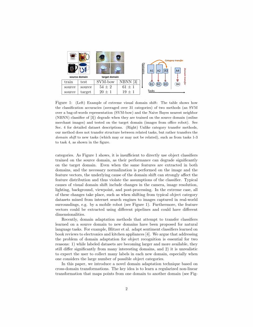
Figure 1: (Left) Example of extreme visual domain shift: The table shows how

the classification accuracies (averaged over 31 categories) of two methods (an SVM

over a bag-of-words representation (SVM-bow) and the Naive Bayes nearest neighbor

(NBNN) classifier of [3]) degrade when they are trained on the source domain (online

merchant images) and tested on the target domain (images from office robot). See

Sec. 4 for detailed dataset descriptions. (Right) Unlike category transfer methods,

our method does not transfer structure between related tasks, but rather transfers the

domain shift to new tasks (which may or may not be related), such as from tasks 1-3

to task 4, as shown in the figure.

categories. As Figure 1 shows, it is insufficient to directly use object classifierstrained on the source domain, as their performance can degrade significantlyon the target domain. Even when the same features are extracted in bothdomains, and the necessary normalization is performed on the image and thefeature vectors, the underlying cause of the domain shift can strongly affect thefeature distribution and thus violate the assumptions of the classifier. Typicalcauses of visual domain shift include changes in the camera, image resolution,lighting, background, viewpoint, and post-processing. In the extreme case, allof these changes take place, such as when shifting from typical object categorydatasets mined from internet search engines to images captured in real-worldsurroundings, e.g. by a mobile robot (see Figure 1). Furthermore, the featurevectors could be extracted using different pipelines and could have differentdimensionalities.

Recently, domain adaptation methods that attempt to transfer classifierslearned on a source domain to new domains have been proposed for naturallanguage tasks. For example, Blitzer et al. adapt sentiment classifiers learned onbook reviews to electronics and kitchen appliances [4]. We argue that addressingthe problem of domain adaptation for object recognition is essential for tworeasons: 1) while labeled datasets are becoming larger and more available, theystill differ significantly from many interesting domains, and 2) it is unrealisticto expect the user to collect many labels in each new domain, especially whenone considers the large number of possible object categories.

In this paper, we introduce a novel domain adaptation technique based oncross-domain transformations. The key idea is to learn a regularized non-lineartransformation that maps points from one domain to another domain (see Fig-

2

ure 2), using supervised data from both domains. The input consists of pairs ofinter-domain examples that are known to be similar (or dissimilar). The out-put is the learned transformation, which can be applied to previously unseentest data points. We present a general model for learning linear cross-domaintransformations, and then prove a novel result showing how to learn non-lineartransformations by kernelizing the formulation for a particular class of regular-izers. The ability to learn asymmetric and non-linear transformations is key, asit allows us to handle more general types of domain shift and changes in featuretype and dimension. Encoding the domain invariance into the feature repre-sentation allows our method to benefit a broad range of classification methods,from k-NN to SVM, as well as clustering methods.

Importantly, our approach can be applied to the scenario where some ofcategories do not have any labels in the target domain. This essentially meanstransferring the learned “domain shift” to new categories encountered in thetarget domain. Thus, our approach can be thought of as a form of knowledgetransfer from the source to the target domain. However, in contrast to manyexisting transfer learning paradigms (e.g. [5], [6]), we do not presume any degreeof relatedness between the categories that are used to learn the transferredstructure and the categories to which the structure is transferred (see Figure 1).The key point is that we are transferring the structure of the domain shift, nottransferring structures common to related categories.

In the next section, we relate our approach to existing work on domainadaptation. Section 3 describes the theoretical framework behind our approach,including novel results on the possibility of kernelization of the asymmetrictransform, and presents the main algorithm. We evaluate our method on a newdataset designed to study the problem of visual domain shift, which is describedin Section 4, and show results of object classifier adaptation on several types ofvisual domain shift in Section 5.

2 Related Work

The domain adaptation problem has recently started to gain attention in thenatural language community. Daume III [7] proposed a domain adaptationapproach that works by transforming the features into an augmented space,where the input features from each domain are copied twice, once to a domain-independent portion of the feature vector, and once to the portion specific tothat domain. The portion specific to all other domains is set to zeros. While“frustratingly” easy to implement, this approach only works for classifiers thatlearn a function over the features. With normalized features (as in our ex-perimental results), the nearest neighbor classifier results are unchanged afteradaptation. Structural correspondence learning is another method proposed forNLP tasks such as sentiment classification [4]. However, it is targeted towardslanguage domains, and relies heavily on the selection of pivot features, whichare words that frequently occur in both domains (e.g. “wonderful”, “awful”)and are correlated with domain-specific words.

3

(a) Domain shift prob-lem

(b) Pairwise con-straints

(c) Invariant space

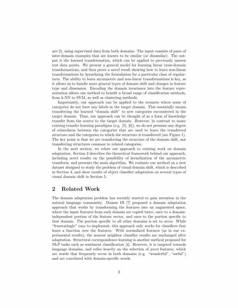
Figure 2: The key idea of our approach to domain adaptation is to learn a transforma-

tion that compensates for the domain-induced changes. By leveraging (dis)similarity

constraints (b) we aim to reunite samples from two different domains (blue and green)

in a common invariant space (c) in order to learn and classify new samples more ef-

fectively across domains. The transformation can also be applied to new categories

(lightly-shaded stars). This figure is best viewed in color.

Recently, several adaptation methods for the support vector machine (SVM)classifier have been proposed in the video retrieval literature. Yang et al. [8]proposed an Adaptive SVM (A-SVM) which adjusts the existing classifier fs(x)trained on the source domain to obtain a new SVM classifier f t(x). Cross-domain SVM (CD-SVM) proposed by Jiang et al. [9] defines a weight for eachsource training sample based on distance to the target domain, and re-trains theSVM classifier was with re-weighted patterns. The domain transfer SVM (DT-SVM) proposed by Duan et al. [10] used multiple-kernel learning to minimizethe difference between the means of the source and target feature distributions.These methods are specific to the SVM classifier, and they require target-domainlabels for all categories. The advantage of our method is that it can performtransfer of domain-invariant representations to novel categories, with no target-domain labels.

Finally, metric and similarity learning has been successfully applied to a va-riety of problems in vision and other domains (see [11, 12, 13, 14] for some visionexamples) but to our knowledge has not been applied to domain adaptation.

3 Domain Adaptation Using Regularized Cross-Domain Transforms

We begin by describing our general domain adaptation model in the linearsetting, focusing on the particular cases that we employ in our experiments,then, in Section 3.1, we prove a novel result showing that kernelization of themodel can be achieved under a wide class of regularizers.

In the following, we assume that there are two domains A and B (e.g.,source and target). Given vectors x ∈ A and y ∈ B, we propose to learn alinear transformation W from B to A (or equivalently, a transformation WT totransform from A to B). If the dimensionality of the vectors x ∈ A is dA andthe dimensionality of the vectors y ∈ B is dB , then the size of the matrix W is

4

dA × dB . We denote the resulting inner product similarity function between xand the transformed y as

simW (x,y) = xTWy.

The goal is to learn the linear transformation given some form of supervision,and then to utilize the learned similarity function in a classification or cluster-ing algorithm. To avoid overfitting, we choose a regularization function for W ,which we will denote as r(W ) (choices of the regularizer are discussed below).Denote X = [x1, ...,xnA

] as the matrix of nA training data points (of dimen-sionality dA) from A and Y = [y1, ...,ynB

] as the matrix of nB training datapoints (of dimensionality dB) from B. We will discuss the exact form of super-vision we propose for domain adaptation problems in Section 3.2, but for nowassume that it is a function of the learned similarity values simW (x,y) (i.e., afunction of the matrix XTWY ), so a general optimization problem would seekto minimize the regularizer subject to supervision constraints given by functionsci:

minW r(W )s.t. ci(X

TWY ) ≥ 0, 1 ≤ i ≤ c. (1)

Due to the potential of infeasibility, we can introduce slack variables into theabove formulation, or write the problem as an unconstrained problem:

minW

r(W ) + λ∑

i

ci(XTWY ).

In this paper, we focus on two particular special cases of this general transfor-mation learning problem. The first employs the regularizer r(W ) = 1

2‖W‖2F and

constraints of the form simW (x,y) ≤ b for dissimilar pairs or simW (x,y) ≥ bfor similar pairs.1 We call this probelm the Frobenius-regularized asymmetrictransformation problem with similarity and dissimilarity constraints, or asymmfor short in the rest of the paper.

Second, we consider the regularizer r(W ) = tr(W ) − log det(W ), and con-straints that are a function of the learned distances dW (x,y) = (x−y)TW (x−y) (as with similarity constraints, the learned distances are linear functionsof XTWY ). Unlike the asymm formulation, this regularizer can only be ap-plied when the dimensionalities of the two domains are equal (dA = dB). Thischoice of regularizer and constraints has previously been studied as a Maha-lanobis metric learning method, and is called information-theoretic metric learn-ing (ITML) [13]; we stress, however, that the use of such a regularizer for domainadaptation is novel, as is our method for constructing cross-domain constraints,which we discuss in Section 3.2. We call this approach symm for short, sincethe learned transformation W is always symmetric positive definite.

1simW (xi,yj) for some xi ∈ A and yj ∈ B can be written as a linear function of XTWYvia the expression eTi XTWY ej , where ei and ej are the i-th and j-th standard basis vectors,respectively.

5

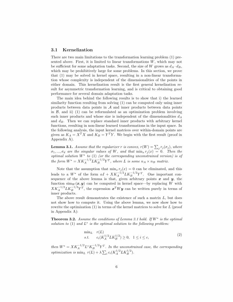
3.1 Kernelization

There are two main limitations to the transformation learning problem (1) pre-sented above. First, it is limited to linear transformations W , which may notbe sufficient for some adaptation tasks. Second, the size of W grows as dA · dB ,which may be prohibitively large for some problems. In this section, we provethat (1) may be solved in kernel space, resulting in a non-linear transforma-tion whose complexity is independent of the dimensionalities of the points ineither domain. This kernelization result is the first general kernelization re-sult for asymmetric transformation learning, and is critical to obtaining goodperformance for several domain adaptation tasks.

The main idea behind the following results is to show that i) the learnedsimilarity function resulting from solving (1) can be computed only using innerproducts between data points in A and inner products between data pointsin B, and ii) (1) can be reformulated as an optimization problem involvingsuch inner products and whose size is independent of the dimensionalities dAand dB . Then we can replace standard inner products with arbitrary kernelfunctions, resulting in non-linear learned transformations in the input space. Inthe following analysis, the input kernel matrices over within-domain points aregiven as KA = XTX and KB = Y TY . We begin with the first result (proof inAppendix A).

Lemma 3.1. Assume that the regularizer r is convex, r(W ) =∑

j rj(σj), whereσ1, ..., σd are the singular values of W , and that minx rj(x) = 0. Then theoptimal solution W ∗ to (1) (or the corresponding unconstrained version) is of

the form W ∗ = XK−1/2A LK

−1/2B Y T , where L is some nA × nB matrix.

Note that the assumption that minx rj(x) = 0 can be eliminated, and this

leads to a W ∗ of the form αI + XK−1/2A LK

−1/2B Y T . One important con-

sequence of the above lemma is that, given arbitrary points x and y, thefunction simW (x,y) can be computed in kernel space—by replacing W with

XK−1/2A LK

−1/2B Y T , the expression xTWy can be written purely in terms of

inner products.The above result demonstrates the existence of such a matrix L, but does

not show how to compute it. Using the above lemma, we now show how torewrite the optimization (1) in terms of the kernel matrices to solve for L (proofin Appendix A):

Theorem 3.2. Assume the conditions of Lemma 3.1 hold. If W ∗ is the optimalsolution to (1) and L∗ is the optimal solution to the following problem:

minL r(L)

s.t. ci(K1/2A LK

1/2B ) ≥ 0, 1 ≤ i ≤ c,

(2)

then W ∗ = XK−1/2A L∗K

−1/2B Y T . In the unconstrained case, the corresponding

optimization is minL r(L) + λ∑

i ci(K1/2A LK

1/2B ).

6

In summary, we have proven that the general asymmetric transformationlearning problem may be applied in kernel space under a class of convex reg-ularizers of the form r(W ) =

∑j rj(σj). Though our focus on this paper is

on two particular regularizers—the squared Frobenius norm and a LogDet-typeregularizer (for the symmetric case)—one can imagine applying our analysis toother regularizers. For example, the trace norm tr(W ) falls under our frame-work; because the trace-norm as a regularizer is known to produce low-rankmatrices W , it would be desirable in dimensionality-reduction settings.

3.2 Algorithm

Both regularizers considered in our paper (r(W ) = 12‖W‖

2F and r(W ) = tr(W )−

log det(W )) are strictly convex, and the constraints we consider are linear. Ineither case, one can use a variety of possible optimization techniques. We optedfor an alternating projection method using Bregman’s algorithm; this methodcan be easily implemented to scale to large problems and has fast convergencein practice. See Censor and Zenios for details on Bregman’s algorithm [15].

Generating Cross-Domain Constraints: Assume that there are k cate-gories, with data from each category i denoted as Di, consisting of (x, y) pairsof input data and category labels. There are two cases that we consider. In thefirst case, we have many labeled examples for each of the n categories in thesource domain data, Ds = {Ds

1, ..., Dsn}, and a few labeled examples for each

category in the target domain data, Dt = {Dt1, ..., D

tn}. In the second case, we

have the same Ds but only have labels for a subset of the categories in the targetdomain, Dt = {Dt

1, ..., Dtm}, where m < k. Here, our goal is to adapt the clas-

sifier trained on the tasks m+ 1, ..., k, which only have source domain labels, toobtain a new classifier, which reduces the predictive error on the target domainby accounting for the domain shift. We do this by applying the transformationlearned on the m categories to the features in the source domain training set ofthe new categories, and re-training the classifier.

To generate similarity constraints (xi,xj) ∈ S and dissimilarity constraints(xi,xj) ∈ D necessary to learn the domain-invariant transformation, we use thefollowing procedure. We sample a random pair consisting of a labeled sourcedomain sample (xs

i , ysi ) and a labeled target domain sample (xt

j , ytj), and create

a constraint

simW (xi,xj) ≥ u if yi = yj ,

simW (xi,xj) ≤ ` if yi 6= yj .(3)

when running asymm and

dW (xi,xj) ≤ u if yi = yj ,

dW (xi,xj) ≥ ` if yi 6= yj .(4)

when running symm. Alternatively, we can generate constraints based not onclass labels, but on information of the form: target sample xi is similar to sourcesample xj . This is particularly useful when the source and target data include

7

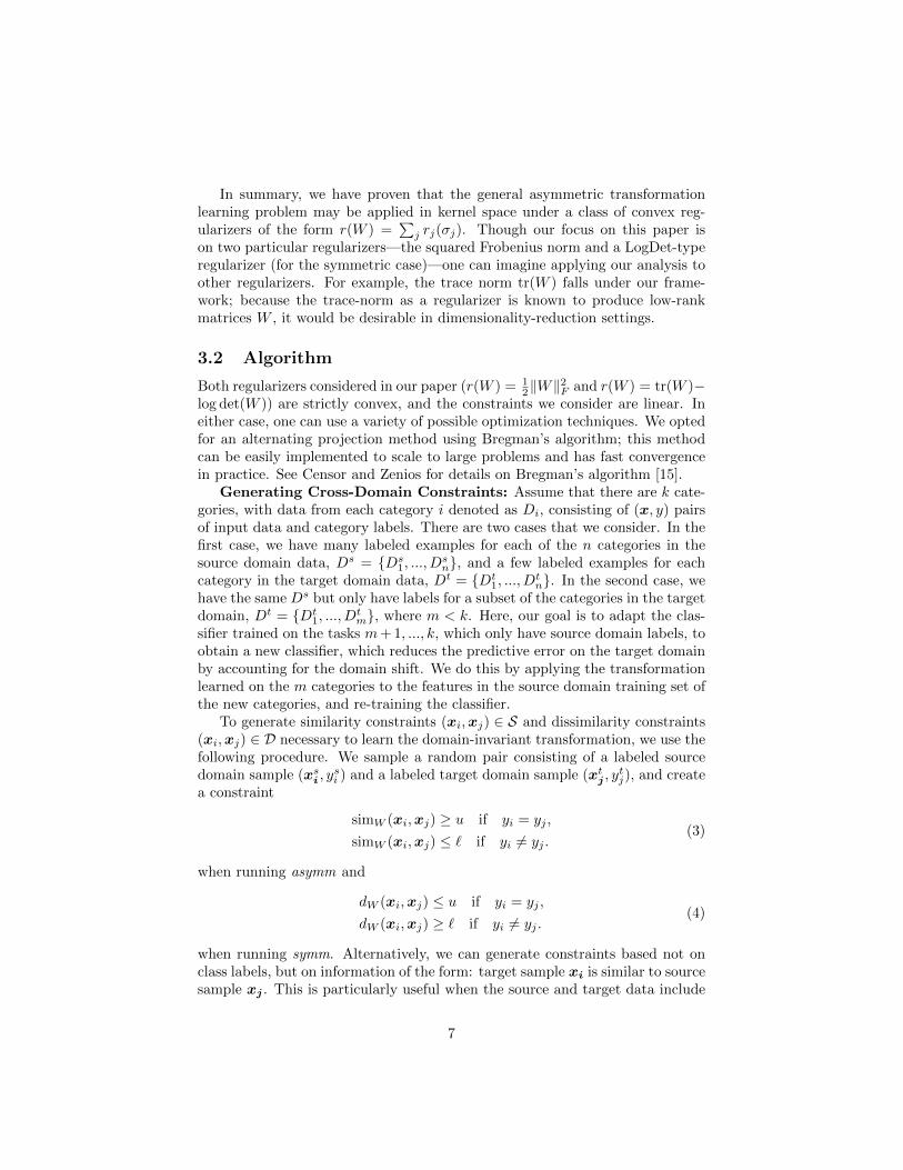
31 categories� �� �

keyboardheadphonesfile cabinet... laptop letter tray ...

amazon dSLR webcam

...

inst

ance

1

...

...

inst

ance

5...

inst

ance

1

...

inst

ance

5

� �� �3 domains

...

...

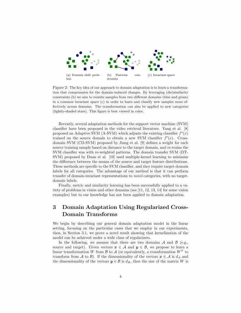
Figure 3: New dataset for investigating domain shifts in visual category recognition

tasks.

images of the same object, as it allows us to best recover the structure of thedomain shift, without learning anything about particular categories. We referto these as correspondence constraints. It is important to generate constraintsbetween samples of different domains, as including same-domain constraints canmake it difficult for the algorithm to learn a domain-invariant metric. In fact, weshow experimentally that generating constraints based on class labels withoutregard for domain boundaries, in the style of metric learning, does considerablyworse than our method.

4 A Database for Studying Effects of DomainShift in Object Recognition

As detailed earlier, effects of domain shift have been largely overlooked in previ-ous object recognition studies. Therefore, one of the contributions of this paperis a database that allows researchers to study, evaluate and compare solutionsto the domain shift problem by establishing a multiple-domain labeled datasetand benchmark. The database, benchmark code, and code for our method willbe made available to the community upon publication. In addition to the do-main shift aspects, this database also proposes a challenging office environmentcategory learning task which reflects the difficulty of real-world indoor roboticobject recognition, and may serve as a useful testbed for such tasks. It containsa total of 4652 images originating from the following three domains:

Images from the web: The first domain consists of images from the webdownloaded from online merchants (www.amazon.com). This has become a verypopular way to acquire data, as it allows for easy access to large amounts of datathat lends itself to learning category models. These images are of products shotat medium resolution typically taken in an environment with studio lighting

8

conditions. We collected two datasets: amazon contains 31 categories2 with anaverage of 90 images each. The images capture the large intra-class variation ofthese categories, but typically show the instances only from a canonical view-point. amazonINS contains 17 object instances (e.g. can of Taster’s Choiceinstant coffee) with an average of two images each.

Images from a digital SLR camera: The second domain consists of im-ages that are captured with a digital SLR camera in realistic environments withnatural lighting conditions. The images have high resolution (4288x2848) andlow noise. We have recorded two datasets: dslr has images of the 31 object cat-egories, with 5 different objects for each, in an office environment. Each objectwas captured with on average 3 images taken from different viewpoints, for atotal of 423 images. dslrINS contains 534 images of the 17 object instances,with an average of 30 images per instance, taken in a home environment.

Images from a webcam: The third domain consists of images of the 31categories recorded with a simple webcam. The images are of low resolution(640x480) and show significant noise and color as well as white balance arti-facts. Many current imagers on robotic platforms share a similarly-sized sensor,and therefore also possess these sensing characteristics. The resulting webcamdataset contains same 5 objects as for in dSLR, for a total of 795 images.

The database represents several interesting visual domain shifts. First of all,it allows us to investigate the adaptation of category models learned on the webto dSLR and webcam images, which can be thought of as in situ observationson a robotic platform in a realistic office or home environment. Second, domaintransfer between the high-quality dSLR images to low-resolution webcam im-ages allows for a very controlled investigation of category model adaptation, asthe same objects were recorded in both domains. Finally, the amazonINS anddslrINS datasets allow us to evaluate adaptation of product instance modelsfrom web data to a user environment, in a setting where images of the sameproducts are available in both domains.

5 Experiments

In this section, we evaluate our domain adaptation approach by applying it tok-nearest neighbor classification of object categories and instances. We use thedatabase described in the previous section to study different types of domainshifts and compare our new approach to several baseline methods. First, wewill detail our processing pipeline before we describe the different setting andelaborate on our empirical findings.

Image Processing: All images were resized to the same width and con-verted to grayscale. Local scale-invariant interest points were detected usingthe SURF [16] detector to describe the image. SURF features have been shown

2The 31 categories in the database are: backpack, bike, bike helmet, bookcase, bottle,calculator, desk chair, desk lamp, computer, file cabinet, headphones, keyboard, laptop, lettertray, mobile phone, monitor, mouse, mug, notebook, pen, phone, printer, projector, puncher,ring binder, ruler, scissors, speaker, stapler, tape, and trash can.

9

No shift Baseline Methods Our Method

domain A domain B knnAA knnAB knnBB ITML(A+B) ITML(B) asymm symm

webcam dslr 0.34 0.14 0.20 0.18 0.23 0.25 0.27dslr webcam 0.31 0.25 0.23 0.23 0.28 0.30 0.31amazon webcam 0.33 0.03 0.43 0.41 0.43 0.48 0.44

Table 1: Domain adaptation results for categories seen during training in thetarget domain.

Baseline Methods Our Method

domain A domain B knnAB ITML(A+B) asymm symm

webcam dslr 0.37 0.38 0.53 0.49webcam-800 dslr-600 0.31 n/a 0.43 n/aamazonINS dslrINS 0.23 0.25 0.30 0.25

Table 2: Domain adaptation results for categories not seen during training inthe target domain.

to be highly repeatable and robust to noise, displacement, geometric and pho-tometric transformations. The blob response threshold was set to 1000, and theother parameters to default values. A 64-dimensional non-rotationally invari-ant SURF descriptor was used to describe the patch surrounding each detectedinterest point. After extracting a set of SURF descriptors for each image, vec-tor quantization into visual words was performed to generate the final featurevector. A codebook of size 800 was constructed by k-means clustering on arandomly chosen subset of the amazon database. All images were converted tohistograms over the resulting visual words. No spatial or color information wasincluded in the image representation for these experiments.

In the following, we compare k-NN classifiers that use the proposed cross-domain transformation to the following baselines: 1) k-NN classifiers that op-erate in the original feature space using a Euclidean distance, and 2) k-NNclassifiers that use traditional supervised metric learning, implemented usingthe ITML [17] method, trained using all available labels in both domains. Wekernelize the metric using an RBF kernel with width σ = 1.0, and set λ = 102.As a performance measure, we use accuracy (number of correctly classified testsamples divided by the total number of test samples) averaged over 10 randomlyselected train/test sets.

Same-category setting: In this setting, all categories have (a small num-ber of) labels in the target domain (3 in our experiments.) We generate con-straints between all cross-domain image pairs in the training set based on theirclass labels, as described in Section 3.2. Table 1 shows the results. In the firstresult column, to illustrate the level of performance without the domain shift, weplot the accuracy of the Euclidean k-NN classifier trained on the source domainA and tested on images from the same domain (knn AA). The next columnshows the same classifier, but trained on A and tested on B (knn AB). Here,

10

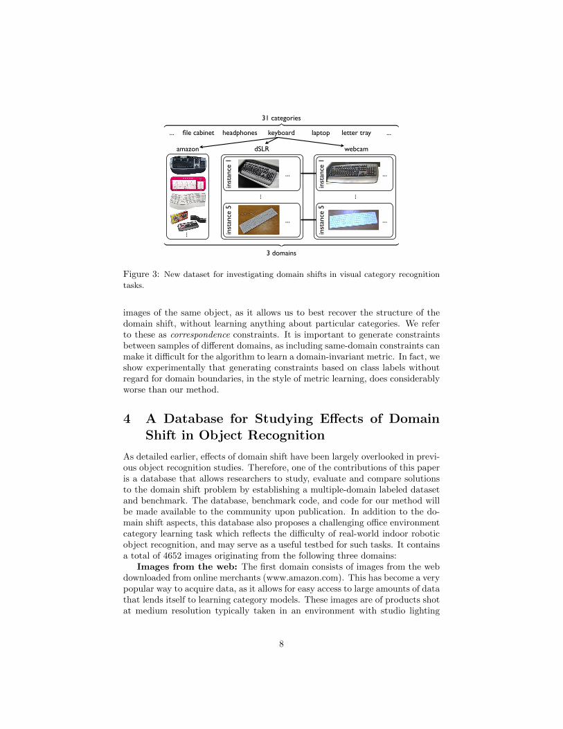
Figure 4: Examples of the 5 nearest neighbors retrieved for a webcam query image

(right image) from the amazon dataset, using the knn AB baseline in Table 1 (top

row of smaller images) and the learned cross-domain symm kernel (bottom row).

the effect of the domain shift is evident, as the performance drops for all do-main pairs, dramatically so in the case of the amazon to webcam shift. We canalso train k-NN using the few available B labels (knn BB, third column). Thefourth and the fifth columns show the metric learning baseline, trained either onall pooled training data from both domains (ITML(A+B), or only on B labels(ITML(B)). The last two columns show the symmetric and asymmetric vari-ants of our domain adaptation method. Note that knn BB does not performas well because of the limited amount of labeled examples we have availablein B. Even the more powerful metric-learning based classifier fails to performas well as the k-NN classifier using our domain-invariant transform, given thesmall amount of labeled target data.

The shift between dslr and webcam domains represents a moderate amountof change, mostly due to the differences in the cameras, as the same objectswere used to collect both datasets. Since webcam actually has more trainingimages, the reverse webcam-to-dslr shift is probably better suited to adaptation.In both these cases, symm outperforms asym, possibly due to the more sym-metric nature of the shift and/or lack of training data to learn a more generaltranformation. The shift between the amazon and the dslr/webcam domainsis the most drastic (bottom row of Table 1.) Even for this challenging prob-lem, the adapted k-NN classifier outperforms the non-adapted baselines, withasymm doing better than symm. Figure 4 show example images retrieved byour method from amazon for a query from webcam.

New-category setting: In this setting, the test data belong to categories(or instances) for which we only have labels in the source domain. We use thefirst half of the categories to learn the transformation, forming correspondenceconstraints between images of the same object instances in roughly the samepose. We test the metric on the remaining categories. The results of adaptingwebcam to dslr are shown the first row of Table 2. Our approach clearly learnssomething about the domain shift, significantly improving the performance overthe baselines, with asymm beating symm. Note that the overall accuracies arehigher as this is a 16-way classification task. The second row in Table 2 showsresults of adapting between heterogeneous feature sets: webcam, where featuresare computed using an 800-codeword vocabulary, and dslr-600, where a different

11

vocabulary is used, with 600 codewords computed on dSLR images. The baselinek-NN is achieved by mapping each B codeword to it’s nearest neighbor in A.This clearly illustrates the advantage of our asymmetric method, as it is able tohandle such drastic transformations of the input features. The last row showsresults on an instance classification task, tackling the shift from Amazon to userenvironment images.

6 Conclusion

We presented a detailed study of domain shift in the context of object recogni-tion, and introduced a novel adaptation technique that projects the features intoa domain-invariant space via a transformation learned from labeled source andtarget domain examples. Our approach can be applied to adapt a wide range ofvisual models which operate over similarities between samples, and works bothon cases where we need to classify novel test samples from categories seen attraining time, and on cases where the test samples come from new categorieswhich were not seen at training time. This is especially useful for object recog-nition, as large multi-category object databases can be adapted to new domainswithout requiring labels for all of the possibly huge number of categories. Ourresults show the effectiveness of our technique for adapting k-NN classifiers toa range of domain shifts.

References

[1] Bosch, A., Zisserman, A., Munoz, X.: Representing shape with a spatialpyramid kernel. In: CIVR. (2007)

[2] Varma, M., Ray, D.: Learning the discriminative power-invariance trade-off. In: ICCV. (2007)

[3] Boiman, O., Shechtman, E., Irani, M.: In defense of nearest-neighbor basedimage classification. In: Proceedings of IEEE Conference on ComputerVision and Pattern Recognition, IEEE (2008)

[4] Blitzer, J., Dredze, M., Pereira, F.: Biographies, bollywood, boom-boxesand blenders: Domain adaptation for sentiment classification. ACL (2007)

[5] Stark, M., Goesele, M., Schiele, B.: A shape-based object class model forknowledge transfer. In: ICCV. (2009)

[6] Fink, M.: Object classification from a single example utilizing class rele-vance metrics. In: Proc. NIPS. (2004)

[7] Daume III, H.: Frustratingly easy domain adaptation. In: ACL. (2007)

[8] Yang, J., Yan, R., Hauptmann, A.G.: Cross-domain video concept detec-tion using adaptive svms. ACM Multimedia (2007)

12

[9] Jiang, W., Zavesky, E., Chang, S., Loui, A.: Cross-domain learning meth-ods for high-level visual concept classification. In: ICIP. (2008)

[10] Duan, L., Tsang, I.W., Xu, D., Maybank, S.J.: Domain transfer svm forvideo concept detection. In: CVPR. (2009)

[11] Chopra, S., Hadsell, R., LeCun, Y.: Learning a similarity metric discrimi-natively, with application to face verification. In: Proc. CVPR. (2005)

[12] Hertz, T., Bar-Hillel, A., Weinshall, D.: Learning distance functions forimage retrieval. In: CVPR. (2004)

[13] Kulis, B., Jain, P., Grauman, K.: Fast similarity search for learned metrics.IEEE PAMI 39 (2009) 2143–2157

[14] Chechik, G., Sharma, V., Shalit, U., Bengio, S.: Large scale online learn-ing of image similarity through ranking. Pattern Recognition and ImageAnalysis (2009)

[15] Censor, Y., Zenios, S.A.: Parallel Optimization: Theory, Algorithms, andApplications. Oxford University Press (1997)

[16] Bay, H., Tuytelaars, T., Van Gool, L.: Surf: Speeded up robust features.In: ECCV. (2006)

[17] Davis, J., Kulis, B., Jain, P., Sra, S., Dhillon, I.: Information-theoreticmetric learning. ICML (2007)

13

A Appendix: Proofs

Proof of Lemma 3.1: Let W have singular value decomposition UΣUT . Wecan therefore write W as W =

∑j σjuju

Tj . For every uj , either it is in the range

space of X or the null space of X. If it is in the range space, then uj = Xzj ,for some zj ; if it is in the null space, then XTuj = 0. An analogous statementholds for uj .

Consider computation of ci(XTWY ). Expanding W via the SVD yields

XTWY = XT

(∑

j

σjujuTj

)Y =

∑

j

σj(XTuju

Tj Y ).

If either uj is in the null space of X or uj is in the null space of Y , thenthe corresponding terms in the sum will be zero. As a result, σj is completelyunconstrained, and can be chosen to minimize fj , which is assumed to be at 0.

Therefore, let us assume that the singular values are ordered such that thefirst t are such that the corresponding singular vectors u are in the range spaceof X and u are in the range space of Y . The remainder of the singular valuesare equal to 0. Then we have

W =

t∑

j=1

σjujuTj =

t∑

j=1

σjXzj zTj Y

T

= X

( t∑

j=1

σjzj zTj

)Y T = XLY T .

With the transformation L = K1/2A LK

1/2B , we can equivalently write as W =

XK−1/2A LK

−1/2B Y T .

Proof of Theorem 3.2: Denote VA = XK−1/2A and VB = Y K

−1/2B . Note

that VA and VB are orthogonal matrices. From the lemma, W = VALVTB ; let

V ⊥A and V ⊥B be the orthogonal complements to VA and VB , and let VA = [VAV⊥V ]

and VB = [VBV⊥B ]. Then

r

(VA

[L 00 0

]VB

T)

= r

([W 00 0

])= r(W ) + const.

One can easily verify that, given two orthogonal matrices V1 and V2 and anarbitrary matrix M , that r(V1MV2) =

∑j rj(σj) if σj are the singular values

of M . So

r

(VA

[L 00 0

]VB

T)

=∑

j

rj(σj) + const = r(L) + const,

where σi are the singular values of L. Thus, r(W ) = r(L) + const.

14

Now rewrite the constraints ci using W = XK−1/2A LK

−1/2B Y T :

ci(XTWY ) = ci(KAK

−1/2A LK

−1/2B KB) = ci(K

1/2A LK

1/2B ).

The theorem follows by rewriting r and the ci functions using the above deriva-tions. Note that both r and the ci’s can be computed independently of thedimensionality, so simple arguments show that the optimization may be solvedin polynomial time independent of the dimensionality when the rj functions areconvex.

15