unsupervised domain adaptation by backpropagationproceedings.mlr.press/v37/ganin15.pdf ·...

Unsupervised Domain Adaptation by Backpropagation

Yaroslav Ganin [email protected] Lempitsky [email protected]

Skolkovo Institute of Science and Technology (Skoltech), Moscow Region, Russia

AbstractTop-performing deep architectures are trained onmassive amounts of labeled data. In the absenceof labeled data for a certain task, domain adap-tation often provides an attractive option giventhat labeled data of similar nature but from a dif-ferent domain (e.g. synthetic images) are avail-able. Here, we propose a new approach to do-main adaptation in deep architectures that canbe trained on large amount of labeled data fromthe source domain and large amount of unlabeleddata from the target domain (no labeled target-domain data is necessary).

As the training progresses, the approach pro-motes the emergence of “deep” features that are(i) discriminative for the main learning task onthe source domain and (ii) invariant with respectto the shift between the domains. We show thatthis adaptation behaviour can be achieved in al-most any feed-forward model by augmenting itwith few standard layers and a simple new gra-dient reversal layer. The resulting augmentedarchitecture can be trained using standard back-propagation.

Overall, the approach can be implemented withlittle effort using any of the deep-learning pack-ages. The method performs very well in a se-ries of image classification experiments, achiev-ing adaptation effect in the presence of big do-main shifts and outperforming previous state-of-the-art on Office datasets.

1. IntroductionDeep feed-forward architectures have brought impressiveadvances to the state-of-the-art across a wide variety ofmachine-learning tasks and applications. At the moment,however, these leaps in performance come only when a

Proceedings of the 32nd International Conference on MachineLearning, Lille, France, 2015. JMLR: W&CP volume 37. Copy-right 2015 by the author(s).

large amount of labeled training data is available. At thesame time, for problems lacking labeled data, it may bestill possible to obtain training sets that are big enough fortraining large-scale deep models, but that suffer from theshift in data distribution from the actual data encounteredat “test time”. One particularly important example is syn-thetic or semi-synthetic training data, which may come inabundance and be fully labeled, but which inevitably havea distribution that is different from real data (Liebelt &Schmid, 2010; Stark et al., 2010; Vazquez et al., 2014; Sun& Saenko, 2014).Learning a discriminative classifier or other predictor inthe presence of a shift between training and test distribu-tions is known as domain adaptation (DA). A number ofapproaches to domain adaptation has been suggested in thecontext of shallow learning, e.g. in the situation when datarepresentation/features are given and fixed. The proposedapproaches then build the mappings between the source(training-time) and the target (test-time) domains, so thatthe classifier learned for the source domain can also be ap-plied to the target domain, when composed with the learnedmapping between domains. The appeal of the domainadaptation approaches is the ability to learn a mapping be-tween domains in the situation when the target domain dataare either fully unlabeled (unsupervised domain annota-tion) or have few labeled samples (semi-supervised domainadaptation). Below, we focus on the harder unsupervisedcase, although the proposed approach can be generalized tothe semi-supervised case rather straightforwardly.Unlike most previous papers on domain adaptation thatworked with fixed feature representations, we focus oncombining domain adaptation and deep feature learningwithin one training process (deep domain adaptation). Ourgoal is to embed domain adaptation into the process oflearning representation, so that the final classification de-cisions are made based on features that are both discrim-inative and invariant to the change of domains, i.e. havethe same or very similar distributions in the source and thetarget domains. In this way, the obtained feed-forward net-work can be applicable to the target domain without beinghindered by the shift between the two domains.We thus focus on learning features that combine (i)


discriminativeness and (ii) domain-invariance. This isachieved by jointly optimizing the underlying features aswell as two discriminative classifiers operating on thesefeatures: (i) the label predictor that predicts class labelsand is used both during training and at test time and (ii) thedomain classifier that discriminates between the source andthe target domains during training. While the parameters ofthe classifiers are optimized in order to minimize their erroron the training set, the parameters of the underlying deepfeature mapping are optimized in order to minimize the lossof the label classifier and to maximize the loss of the domainclassifier. The latter encourages domain-invariant featuresto emerge in the course of the optimization.Crucially, we show that all three training processes canbe embedded into an appropriately composed deep feed-forward network (Figure 1) that uses standard layers andloss functions, and can be trained using standard backprop-agation algorithms based on stochastic gradient descent orits modifications (e.g. SGD with momentum). Our ap-proach is generic as it can be used to add domain adaptationto any existing feed-forward architecture that is trainable bybackpropagation. In practice, the only non-standard com-ponent of the proposed architecture is a rather trivial gra-dient reversal layer that leaves the input unchanged duringforward propagation and reverses the gradient by multiply-ing it by a negative scalar during the backpropagation.Below, we detail the proposed approach to domain adap-tation in deep architectures, and present results on tradi-tional deep learning image datasets (such as MNIST (Le-Cun et al., 1998) and SVHN (Netzer et al., 2011)) as wellas on OFFICE benchmarks (Saenko et al., 2010), wherethe proposed method considerably improves over previousstate-of-the-art accuracy.

2. Related workA large number of domain adaptation methods have beenproposed over the recent years, and here we focus on themost related ones. Multiple methods perform unsuper-vised domain adaptation by matching the feature distri-butions in the source and the target domains. Some ap-proaches perform this by reweighing or selecting samplesfrom the source domain (Borgwardt et al., 2006; Huanget al., 2006; Gong et al., 2013), while others seek an ex-plicit feature space transformation that would map sourcedistribution into the target ones (Pan et al., 2011; Gopalanet al., 2011; Baktashmotlagh et al., 2013). An importantaspect of the distribution matching approach is the way the(dis)similarity between distributions is measured. Here,one popular choice is matching the distribution means inthe kernel-reproducing Hilbert space (Borgwardt et al.,2006; Huang et al., 2006), whereas (Gong et al., 2012; Fer-nando et al., 2013) map the principal axes associated witheach of the distributions. Our approach also attempts tomatch feature space distributions, however this is accom-

plished by modifying the feature representation itself ratherthan by reweighing or geometric transformation. Also, ourmethod uses (implicitly) a rather different way to measurethe disparity between distributions based on their separa-bility by a deep discriminatively-trained classifier.Several approaches perform gradual transition from thesource to the target domain (Gopalan et al., 2011; Gonget al., 2012) by a gradual change of the training distribu-tion. Among these methods, (S. Chopra & Gopalan, 2013)does this in a “deep” way by the layerwise training of asequence of deep autoencoders, while gradually replacingsource-domain samples with target-domain samples. Thisimproves over a similar approach of (Glorot et al., 2011)that simply trains a single deep autoencoder for both do-mains. In both approaches, the actual classifier/predictoris learned in a separate step using the feature representa-tion learned by autoencoder(s). In contrast to (Glorot et al.,2011; S. Chopra & Gopalan, 2013), our approach performsfeature learning, domain adaptation and classifier learningjointly, in a unified architecture, and using a single learningalgorithm (backpropagation). We therefore argue that ourapproach is simpler (both conceptually and in terms of itsimplementation). Our method also achieves considerablybetter results on the popular OFFICE benchmark.While the above approaches perform unsupervised domainadaptation, there are approaches that perform superviseddomain adaptation by exploiting labeled data from the tar-get domain. In the context of deep feed-forward archi-tectures, such data can be used to “fine-tune” the net-work trained on the source domain (Zeiler & Fergus, 2013;Oquab et al., 2014; Babenko et al., 2014). Our approachdoes not require labeled target-domain data. At the sametime, it can easily incorporate such data when it is avail-able.An idea related to ours is described in (Goodfellow et al.,2014). While their goal is quite different (building gener-ative deep networks that can synthesize samples), the waythey measure and minimize the discrepancy between thedistribution of the training data and the distribution of thesynthesized data is very similar to the way our architecturemeasures and minimizes the discrepancy between featuredistributions for the two domains.In the recent year, domain adaptation for feed-forward neu-ral networks has attracted a lot of interest. Thus, a verysimilar idea to ours has been developed in parallel and in-dependently for shallow architecture (with a single hiddenlayer) in (Ajakan et al., 2014). Their system is evaluatedon a natural language task (sentiment analysis). Further-more, recent and concurrent reports by (Tzeng et al., 2014;Long & Wang, 2015) also focus on domain adaptation infeed-forward networks. Their set of techniques measuresand minimizes the distance between the data distributionmeans across domains (potentially, after embedding distri-butions into RKHS). The approach of (Tzeng et al., 2014)


Figure 1. The proposed architecture includes a deep feature extractor (green) and a deep label predictor (blue), which together forma standard feed-forward architecture. Unsupervised domain adaptation is achieved by adding a domain classifier (red) connected to thefeature extractor via a gradient reversal layer that multiplies the gradient by a certain negative constant during the backpropagation-based training. Otherwise, the training proceeds in a standard way and minimizes the label prediction loss (for source examples) andthe domain classification loss (for all samples). Gradient reversal ensures that the feature distributions over the two domains are madesimilar (as indistinguishable as possible for the domain classifier), thus resulting in the domain-invariant features.

and (Long & Wang, 2015) is thus different from our ideaof matching distribution by making them indistinguishablefor a discriminative classifier. Below, we compare our ap-proach to (Tzeng et al., 2014; Long & Wang, 2015) on theOffice benchmark. Another approach to deep domain adap-tation, which is arguably more different from ours, has beendeveloped in parallel in (Chen et al., 2015).

3. Deep Domain Adaptation3.1. The modelWe now detail the proposed model for the domain adap-tation. We assume that the model works with input sam-ples x ∈ X , where X is some input space and cer-tain labels (output) y from the label space Y . Below,we assume classification problems where Y is a finite set(Y = {1, 2, . . . L}), however our approach is generic andcan handle any output label space that other deep feed-forward models can handle. We further assume that thereexist two distributions S(x, y) and T (x, y) on X ⊗ Y ,which will be referred to as the source distribution andthe target distribution (or the source domain and the tar-get domain). Both distributions are assumed complex andunknown, and furthermore similar but different (in otherwords, S is “shifted” from T by some domain shift).Our ultimate goal is to be able to predict labels y giventhe input x for the target distribution. At training time,we have an access to a large set of training samples{x1,x2, . . . ,xN} from both the source and the target do-mains distributed according to the marginal distributionsS(x) and T (x). We denote with di the binary variable (do-main label) for the i-th example, which indicates whetherxi come from the source distribution (xi∼S(x) if di=0) orfrom the target distribution (xi∼T (x) if di=1). For the ex-amples from the source distribution (di=0) the correspond-

ing labels yi ∈ Y are known at training time. For the ex-amples from the target domains, we do not know the labelsat training time, and we want to predict such labels at testtime.We now define a deep feed-forward architecture that foreach input x predicts its label y ∈ Y and its domain labeld ∈ {0, 1}. We decompose such mapping into three parts.We assume that the input x is first mapped by a mappingGf (a feature extractor) to a D-dimensional feature vectorf ∈ RD. The feature mapping may also include severalfeed-forward layers and we denote the vector of parame-ters of all layers in this mapping as θf , i.e. f = Gf (x; θf ).Then, the feature vector f is mapped by a mapping Gy (la-bel predictor) to the label y, and we denote the parametersof this mapping with θy . Finally, the same feature vector fis mapped to the domain label d by a mapping Gd (domainclassifier) with the parameters θd (Figure 1).During the learning stage, we aim to minimize the labelprediction loss on the annotated part (i.e. the source part)of the training set, and the parameters of both the featureextractor and the label predictor are thus optimized in or-der to minimize the empirical loss for the source domainsamples. This ensures the discriminativeness of the fea-tures f and the overall good prediction performance of thecombination of the feature extractor and the label predictoron the source domain.At the same time, we want to make the features fdomain-invariant. That is, we want to make the dis-tributions S(f) = {Gf (x; θf ) |x∼S(x)} and T (f) ={Gf (x; θf ) |x∼T (x)} to be similar. Under the covariateshift assumption, this would make the label prediction ac-curacy on the target domain to be the same as on the sourcedomain (Shimodaira, 2000). Measuring the dissimilarityof the distributions S(f) and T (f) is however non-trivial,given that f is high-dimensional, and that the distributions


themselves are constantly changing as learning progresses.One way to estimate the dissimilarity is to look at the lossof the domain classifier Gd, provided that the parametersθd of the domain classifier have been trained to discrim-inate between the two feature distributions in an optimalway.This observation leads to our idea. At training time, in or-der to obtain domain-invariant features, we seek the param-eters θf of the feature mapping that maximize the loss ofthe domain classifier (by making the two feature distribu-tions as similar as possible), while simultaneously seekingthe parameters θd of the domain classifier that minimize theloss of the domain classifier. In addition, we seek to mini-mize the loss of the label predictor.More formally, we consider the functional:

E(θf , θy, θd) =∑i=1..Ndi=0

Ly(Gy(Gf (xi; θf ); θy), yi

)−

λ∑i=1..N

Ld(Gd(Gf (xi; θf ); θd), yi

)=

=∑i=1..Ndi=0

Liy(θf , θy)− λ∑i=1..N

Lid(θf , θd) (1)

Here, Ly(·, ·) is the loss for label prediction (e.g. multino-mial), Ld(·, ·) is the loss for the domain classification (e.g.logistic), while Liy and Lid denote the corresponding lossfunctions evaluated at the i-th training example.Based on our idea, we are seeking the parameters θf , θy, θdthat deliver a saddle point of the functional (1):

(θf , θy) = arg minθf ,θy

E(θf , θy, θd) (2)

θd = arg maxθd

E(θf , θy, θd) . (3)

At the saddle point, the parameters θd of the domain classi-fier θd minimize the domain classification loss (since it en-ters into (1) with the minus sign) while the parameters θy ofthe label predictor minimize the label prediction loss. Thefeature mapping parameters θf minimize the label predic-tion loss (i.e. the features are discriminative), while maxi-mizing the domain classification loss (i.e. the features aredomain-invariant). The parameter λ controls the trade-offbetween the two objectives that shape the features duringlearning.Below, we demonstrate that standard stochastic gradientsolvers (SGD) can be adapted for the search of the saddlepoint (2)-(3).

3.2. Optimization with backpropagationA saddle point (2)-(3) can be found as a stationary point ofthe following stochastic updates:

θf ←− θf − µ

(∂Liy∂θf

− λ∂Lid

∂θf

)(4)

θy ←− θy − µ∂Liy∂θy

(5)

θd ←− θd − µ∂Lid∂θd

(6)

where µ is the learning rate (which can vary over time).The updates (4)-(6) are very similar to stochastic gradientdescent (SGD) updates for a feed-forward deep model thatcomprises feature extractor fed into the label predictor andinto the domain classifier. The difference is the −λ factorin (4) (the difference is important, as without such factor,stochastic gradient descent would try to make features dis-similar across domains in order to minimize the domainclassification loss). Although direct implementation of (4)-(6) as SGD is not possible, it is highly desirable to reducethe updates (4)-(6) to some form of SGD, since SGD (andits variants) is the main learning algorithm implemented inmost packages for deep learning.Fortunately, such reduction can be accomplished by intro-ducing a special gradient reversal layer (GRL) defined asfollows. The gradient reversal layer has no parameters as-sociated with it (apart from the meta-parameter λ, whichis not updated by backpropagation). During the forwardpropagation, GRL acts as an identity transform. Duringthe backpropagation though, GRL takes the gradient fromthe subsequent level, multiplies it by −λ and passes it tothe preceding layer. Implementing such layer using exist-ing object-oriented packages for deep learning is simple, asdefining procedures for forwardprop (identity transform),backprop (multiplying by a constant), and parameter up-date (nothing) is trivial.The GRL as defined above is inserted between the featureextractor and the domain classifier, resulting in the archi-tecture depicted in Figure 1. As the backpropagation pro-cess passes through the GRL, the partial derivatives of theloss that is downstream the GRL (i.e. Ld) w.r.t. the layerparameters that are upstream the GRL (i.e. θf ) get multi-plied by −λ, i.e. ∂Ld

∂θfis effectively replaced with −λ∂Ld

∂θf.

Therefore, running SGD in the resulting model implementsthe updates (4)-(6) and converges to a saddle point of (1).Mathematically, we can formally treat the gradient reversallayer as a “pseudo-function”Rλ(x) defined by two (incom-patible) equations describing its forward- and backpropa-gation behaviour:

Rλ(x) = x (7)dRλdx

= −λI (8)

where I is an identity matrix. We can then define theobjective “pseudo-function” of (θf , θy, θd) that is being


optimized by the stochastic gradient descent within ourmethod:

E(θf , θy, θd) =∑i=1..Ndi=0

Ly(Gy(Gf (xi; θf ); θy), yi

)+

∑i=1..N

Ld(Gd(Rλ(Gf (xi; θf )); θd), yi

)(9)

Running updates (4)-(6) can then be implemented as do-ing SGD for (9) and leads to the emergence of featuresthat are domain-invariant and discriminative at the sametime. After the learning, the label predictor y(x) =Gy(Gf (x; θf ); θy) can be used to predict labels for sam-ples from the target domain (as well as from the sourcedomain).The simple learning procedure outlined above can be re-derived/generalized along the lines suggested in (Goodfel-low et al., 2014) (see the supplementary material (Ganin &Lempitsky, 2015)).

3.3. Relation toH∆H-distanceIn this section we give a brief analysis of our method interms ofH∆H-distance (Ben-David et al., 2010; Cortes &Mohri, 2011) which is widely used in the theory of non-conservative domain adaptation. Formally,

dH∆H(S, T ) = 2 suph1,h2∈H

|Pf∼S [h1(f) 6= h2(f)]−

−Pf∼T [h1(f) 6= h2(f)]| (10)

defines a discrepancy distance between two distributions Sand T w.r.t. a hypothesis set H. Using this notion one canobtain a probabilistic bound (Ben-David et al., 2010) on theperformance εT (h) of some classifier h from T evaluatedon the target domain given its performance εS(h) on thesource domain:

εT (h) ≤ εS(h) +1

2dH∆H(S, T ) + C , (11)

where S and T are source and target distributions respec-tively, and C does not depend on particular h.Consider fixed S and T over the representation space pro-duced by the feature extractor Gf and a family of labelpredictorsHp. We assume that the family of domain classi-fiersHd is rich enough to contain the symmetric differencehypothesis set ofHp:

Hp∆Hp = {h |h = h1 ⊕ h2 , h1, h2 ∈ Hp} . (12)

It is not an unrealistic assumption as we have a freedom topick Hd whichever we want. For example, we can set thearchitecture of the domain discriminator to be the layer-by-layer concatenation of two replicas of the label predic-tor followed by a two layer non-linear perceptron aimed tolearn the XOR-function. Given the assumption holds, one

MNIST SYN NUM SVHN SYN SIGNS

MNIST-M SVHN MNIST GTSRB

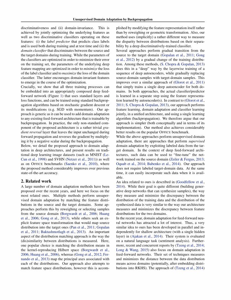
Figure 2. Examples of domain pairs (top – source domain, bot-tom – target domain) used in the small image experiments. SeeSection 4.1 for details.

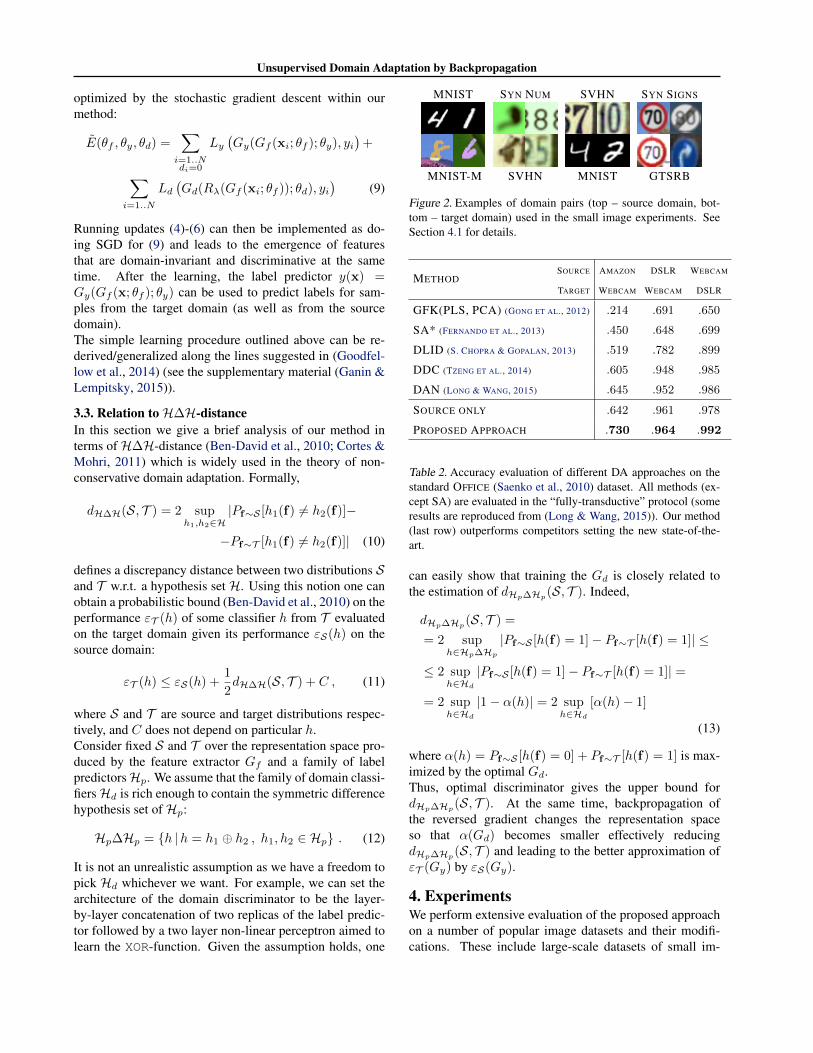
METHODSOURCE AMAZON DSLR WEBCAM

TARGET WEBCAM WEBCAM DSLR

GFK(PLS, PCA) (GONG ET AL., 2012) .214 .691 .650

SA* (FERNANDO ET AL., 2013) .450 .648 .699

DLID (S. CHOPRA & GOPALAN, 2013) .519 .782 .899

DDC (TZENG ET AL., 2014) .605 .948 .985

DAN (LONG & WANG, 2015) .645 .952 .986

SOURCE ONLY .642 .961 .978

PROPOSED APPROACH .730 .964 .992

Table 2. Accuracy evaluation of different DA approaches on thestandard OFFICE (Saenko et al., 2010) dataset. All methods (ex-cept SA) are evaluated in the “fully-transductive” protocol (someresults are reproduced from (Long & Wang, 2015)). Our method(last row) outperforms competitors setting the new state-of-the-art.

can easily show that training the Gd is closely related tothe estimation of dHp∆Hp

(S, T ). Indeed,

dHp∆Hp(S, T ) =

= 2 suph∈Hp∆Hp

|Pf∼S [h(f) = 1]− Pf∼T [h(f) = 1]| ≤

≤ 2 suph∈Hd

|Pf∼S [h(f) = 1]− Pf∼T [h(f) = 1]| =

= 2 suph∈Hd

|1− α(h)| = 2 suph∈Hd

[α(h)− 1]

(13)

where α(h) = Pf∼S [h(f) = 0] + Pf∼T [h(f) = 1] is max-imized by the optimal Gd.Thus, optimal discriminator gives the upper bound fordHp∆Hp

(S, T ). At the same time, backpropagation ofthe reversed gradient changes the representation spaceso that α(Gd) becomes smaller effectively reducingdHp∆Hp(S, T ) and leading to the better approximation ofεT (Gy) by εS(Gy).

4. ExperimentsWe perform extensive evaluation of the proposed approachon a number of popular image datasets and their modifi-cations. These include large-scale datasets of small im-


METHODSOURCE MNIST SYN NUMBERS SVHN SYN SIGNS

TARGET MNIST-M SVHN MNIST GTSRB

SOURCE ONLY .5225 .8674 .5490 .7900

SA (FERNANDO ET AL., 2013) .5690 (4.1%) .8644 (−5.5%) .5932 (9.9%) .8165 (12.7%)

PROPOSED APPROACH .7666 (52.9%) .9109 (79.7%) .7385 (42.6%) .8865 (46.4%)

TRAIN ON TARGET .9596 .9220 .9942 .9980

Table 1. Classification accuracies for digit image classifications for different source and target domains. MNIST-M corresponds todifference-blended digits over non-uniform background. The first row corresponds to the lower performance bound (i.e. if no adaptationis performed). The last row corresponds to training on the target domain data with known class labels (upper bound on the DA perfor-mance). For each of the two DA methods (ours and (Fernando et al., 2013)) we show how much of the gap between the lower and theupper bounds was covered (in brackets). For all five cases, our approach outperforms (Fernando et al., 2013) considerably, and covers abig portion of the gap.

ages popular with deep learning methods, and the OFFICEdatasets (Saenko et al., 2010), which are a de facto standardfor domain adaptation in computer vision, but have muchfewer images.

Baselines. For the bulk of experiments the following base-lines are evaluated. The source-only model is trained with-out consideration for target-domain data (no domain clas-sifier branch included into the network). The train-on-target model is trained on the target domain with classlabels revealed. This model serves as an upper bound onDA methods, assuming that target data are abundant andthe shift between the domains is considerable.In addition, we compare our approach against the recentlyproposed unsupervised DA method based on subspacealignment (SA) (Fernando et al., 2013), which is simpleto setup and test on new datasets, but has also been shownto perform very well in experimental comparisons withother “shallow” DA methods. To boost the performanceof this baseline, we pick its most important free parame-ter (the number of principal components) from the range{2, . . . , 60}, so that the test performance on the target do-main is maximized. To apply SA in our setting, we traina source-only model and then consider the activations ofthe last hidden layer in the label predictor (before the finallinear classifier) as descriptors/features, and learn the map-ping between the source and the target domains (Fernandoet al., 2013).Since the SA baseline requires to train a new classifier afteradapting the features, and in order to put all the comparedsettings on an equal footing, we retrain the last layer ofthe label predictor using a standard linear SVM (Fan et al.,2008) for all four considered methods (including ours; theperformance on the target domain remains approximatelythe same after the retraining).For the OFFICE dataset (Saenko et al., 2010), we directlycompare the performance of our full network (feature ex-tractor and label predictor) against recent DA approaches

using previously published results.

CNN architectures. In general, we compose feature ex-tractor from two or three convolutional layers, picking theirexact configurations from previous works. We give the ex-act architectures in the supplementary material (Ganin &Lempitsky, 2015).For the domain adaptator we stick to the three fully con-nected layers (x → 1024 → 1024 → 2), except forMNIST where we used a simpler (x → 100 → 2) ar-chitecture to speed up the experiments.For loss functions, we set Ly and Ld to be the logistic re-gression loss and the binomial cross-entropy respectively.

CNN training procedure. The model is trained on 128-sized batches. Images are preprocessed by the mean sub-traction. A half of each batch is populated by the sam-ples from the source domain (with known labels), the restis comprised of the target domain (with unknown labels).In order to suppress noisy signal from the domain classifierat the early stages of the training procedure instead of fixingthe adaptation factor λ, we gradually change it from 0 to 1using the following schedule:

λp =2

1 + exp(−γ · p)− 1, (14)

where γ was set to 10 in all experiments (the schedule wasnot optimized/tweaked). Further details on the CNN train-ing can be found in the supplementary material (Ganin &Lempitsky, 2015).

Visualizations. We use t-SNE (van der Maaten, 2013) pro-jection to visualize feature distributions at different pointsof the network, while color-coding the domains (Figure 3).We observe strong correspondence between the success ofthe adaptation in terms of the classification accuracy for thetarget domain, and the overlap between the domain distri-butions in such visualizations.

Choosing meta-parameters. Good unsupervised DA


methods should provide ways to set meta-parameters (suchas λ, the learning rate, the momentum rate, the networkarchitecture for our method) in an unsupervised way, i.e.without referring to labeled data in the target domain. Inour method, one can assess the performance of the wholesystem (and the effect of changing hyper-parameters) byobserving the test error on the source domain and the do-main classifier error. In general, we observed a good cor-respondence between the success of adaptation and theseerrors (adaptation is more successful when the source do-main test error is low, while the domain classifier error ishigh). In addition, the layer, where the the domain discrim-inator is attached can be picked by computing differencebetween means as suggested in (Tzeng et al., 2014).

4.1. ResultsWe now discuss the experimental settings and the results.In each case, we train on the source dataset and test ona different target domain dataset, with considerable shiftsbetween domains (see Figure 2).When MNIST and SVHNdatasets are used as target, standard training-test splits areconsidered, and all training images are used for unsuper-vised adaptation. The results are summarized in Table 1and Table 2.

MNIST → MNIST-M. Our first experiment deals withthe MNIST dataset (LeCun et al., 1998) (source). In or-der to obtain the target domain (MNIST-M) we blend dig-its from the original set over patches randomly extractedfrom color photos from BSDS500 (Arbelaez et al., 2011).This operation is formally defined for two images I1, I2 asIoutijk = |I1

ijk − I2ijk|, where i, j are the coordinates of a

pixel and k is a channel index. In other words, an outputsample is produced by taking a patch from a photo and in-verting its pixels at positions corresponding to the pixels ofa digit. For a human the classification task becomes onlyslightly harder compared to the original dataset (the digitsare still clearly distinguishable) whereas for a CNN trainedon MNIST this domain is quite distinct, as the backgroundand the strokes are no longer constant. Consequently, thesource-only model performs poorly. Our approach suc-ceeded at aligning feature distributions (Figure 3), whichled to successful adaptation results (considering that theadaptation is unsupervised). At the same time, the im-provement over source-only model achieved by subspacealignment (SA) (Fernando et al., 2013) is quite modest,thus highlighting the difficulty of the adaptation task.

Synthetic numbers→ SVHN. To address a common sce-nario of training on synthetic data and testing on real data,we use Street-View House Number dataset SVHN (Netzeret al., 2011) as the target domain and synthetic digits as thesource. The latter (SYN NUMBERS) consists of≈ 500,000images generated by ourselves from WindowsTM fonts byvarying the text (that includes different one-, two-, and

three-digit numbers), positioning, orientation, backgroundand stroke colors, and the amount of blur. The degrees ofvariation were chosen manually to simulate SVHN, how-ever the two datasets are still rather distinct, the biggestdifference being the structured clutter in the background ofSVHN images.The proposed backpropagation-based technique works wellcovering almost 80% of the gap between training withsource data only and training on target domain data withknown target labels. In contrast, SA (Fernando et al., 2013)results in a slight classification accuracy drop (probablydue to the information loss during the dimensionality re-duction), thus indicating that the adaptation task is evenmore challenging than in the case of the MNIST experi-ment.

MNIST↔ SVHN. In this experiment, we further increasethe gap between distributions, and test on MNIST andSVHN, which are significantly different in appearance.Training on SVHN even without adaptation is challeng-ing — classification error stays high during the first 150epochs. In order to avoid ending up in a poor local min-imum we, therefore, do not use learning rate annealinghere. Obviously, the two directions (MNIST → SVHNand SVHN → MNIST) are not equally difficult. AsSVHN is more diverse, a model trained on SVHN is ex-pected to be more generic and to perform reasonably onthe MNIST dataset. This, indeed, turns out to be the caseand is supported by the appearance of the feature distribu-tions. We observe a quite strong separation between thedomains when we feed them into the CNN trained solelyon MNIST, whereas for the SVHN-trained network thefeatures are much more intermixed. This difference prob-ably explains why our method succeeded in improving theperformance by adaptation in the SVHN → MNIST sce-nario (see Table 1) but not in the opposite direction (SA isnot able to perform adaptation in this case either). Unsu-pervised adaptation from MNIST to SVHN gives a failureexample for our approach (we are unaware of any unsuper-vised DA methods capable of performing such adaptation).

Synthetic Signs→GTSRB. Overall, this setting is similarto the SYN NUMBERS → SVHN experiment, except thedistribution of the features is more complex due to the sig-nificantly larger number of classes (43 instead of 10). Forthe source domain we obtained 100,000 synthetic images(which we call SYN SIGNS) simulating various imagingconditions. In the target domain, we use 31,367 randomtraining samples for unsupervised adaptation and the restfor evaluation. Once again, our method achieves a sensi-ble increase in performance proving its suitability for thesynthetic-to-real data adaptation.As an additional experiment, we also evaluate the proposedalgorithm for semi-supervised domain adaptation. Here,we reveal 430 labeled examples (10 samples per class) and


MNIST→ MNIST-M: top feature extractor layer

(a) Non-adapted (b) Adapted

SYN NUMBERS→ SVHN: last hidden layer of the label predictor

(a) Non-adapted (b) Adapted

Figure 3. The effect of adaptation on the distribution of the extracted features (best viewed in color). The figure shows t-SNE (van derMaaten, 2013) visualizations of the CNN’s activations (a) in case when no adaptation was performed and (b) in case when our adaptationprocedure was incorporated into training. Blue points correspond to the source domain examples, while red ones correspond to the targetdomain. In all cases, the adaptation in our method makes the two distributions of features much closer.

0 1 2 3 4 5

·105

0.1

0.15

0.2

Batches seen

Val

idat

ion

erro

r

RealSynSyn AdaptedSyn + RealSyn + Real Adapted

Figure 4. Results for the traffic signs classification in the semi-supervised setting. Syn and Real denote available labeled data(100,000 synthetic and 430 real images respectively); Adaptedmeans that ≈ 31,000 unlabeled target domain images were usedfor adaptation. The best performance is achieved by employingboth the labeled samples and the large unlabeled corpus in thetarget domain.

add them to the training set for the label predictor. Fig-ure 4 shows the change of the validation error through-out the training. While the graph clearly suggests that ourmethod can be beneficial in the semi-supervised setting,thorough verification of semi-supervised setting is left forfuture work.

Office dataset. We finally evaluate our method on OF-FICE dataset, which is a collection of three distinct do-mains: AMAZON, DSLR, and WEBCAM. Unlike previ-ously discussed datasets, OFFICE is rather small-scale withonly 2817 labeled images spread across 31 different cate-gories in the largest domain. The amount of available datais crucial for a successful training of a deep model, hencewe opted for the fine-tuning of the CNN pre-trained on theImageNet (AlexNet from the Caffe package (Jia et al.,2014)) as it is done in some recent DA works (Donahueet al., 2014; Tzeng et al., 2014; Hoffman et al., 2013; Long& Wang, 2015). We make our approach more compara-ble with (Tzeng et al., 2014) by using exactly the samenetwork architecture replacing domain mean-based regu-larization with the domain classifier.Following previous works, we assess the performance ofour method across three transfer tasks most commonlyused for evaluation. Our training protocol is adopted from

(Gong et al., 2013; S. Chopra & Gopalan, 2013; Long &Wang, 2015) as during adaptation we use all available la-beled source examples and unlabeled target examples (thepremise of our method is the abundance of unlabeled datain the target domain). Also, all source domain is usedfor training. Under this “fully-transductive” setting, ourmethod is able to improve previously-reported state-of-the-art accuracy for unsupervised adaptation very considerably(Table 2), especially in the most challenging AMAZON →WEBCAM scenario (the two domains with the largest do-main shift).Interestingly, in all three experiments we observe a slightover-fitting as training progresses, however, it doesn’t ruinthe validation accuracy. Moreover, switching off the do-main classifier branch makes this effect far more apparent,from which we conclude that our technique serves as a reg-ularizer.

5. DiscussionWe have proposed a new approach to unsupervised do-main adaptation of deep feed-forward architectures, whichallows large-scale training based on large amount of an-notated data in the source domain and large amount ofunannotated data in the target domain. Similarly to manyprevious shallow and deep DA techniques, the adaptationis achieved through aligning the distributions of featuresacross the two domains. However, unlike previous ap-proaches, the alignment is accomplished through standardbackpropagation training. The approach is therefore ratherscalable, and can be implemented using any deep learn-ing package. To this end we release the source code forthe Gradient Reversal layer along with the usage examplesas an extension to Caffe (Jia et al., 2014) (see (Ganin &Lempitsky, 2015)). Further evaluation on larger-scale tasksand in semi-supervised settings constitutes future work.Acknowledgements. This research is supported bythe Russian Ministry of Science and Education grantRFMEFI57914X0071. We also thank the Graphics & Me-dia Lab, Moscow State University for providing the syn-thetic road signs data.


ReferencesAjakan, Hana, Germain, Pascal, Larochelle, Hugo, Lavi-

olette, Francois, and Marchand, Mario. Domain-adversarial neural networks. CoRR, abs/1412.4446,2014.

Arbelaez, Pablo, Maire, Michael, Fowlkes, Charless, andMalik, Jitendra. Contour detection and hierarchical im-age segmentation. PAMI, 33, 2011.

Babenko, Artem, Slesarev, Anton, Chigorin, Alexander,and Lempitsky, Victor S. Neural codes for image re-trieval. In ECCV, pp. 584–599, 2014.

Baktashmotlagh, Mahsa, Harandi, Mehrtash Tafazzoli,Lovell, Brian C., and Salzmann, Mathieu. Unsuperviseddomain adaptation by domain invariant projection. InICCV, pp. 769–776, 2013.

Ben-David, Shai, Blitzer, John, Crammer, Koby, Kulesza,Alex, Pereira, Fernando, and Vaughan, Jennifer Wort-man. A theory of learning from different domains.JMLR, 79, 2010.

Borgwardt, Karsten M., Gretton, Arthur, Rasch, Malte J.,Kriegel, Hans-Peter, Scholkopf, Bernhard, and Smola,Alexander J. Integrating structured biological data bykernel maximum mean discrepancy. In ISMB, pp. 49–57, 2006.

Chen, Qiang, Huang, Junshi, Feris, Rogerio, Brown,Lisa M., Dong, Jian, and Yan, Shuicheng. Deep domainadaptation for describing people based on fine-grainedclothing attributes. June 2015.

Cortes, Corinna and Mohri, Mehryar. Domain adaptationin regression. In Algorithmic Learning Theory, 2011.

Donahue, Jeff, Jia, Yangqing, Vinyals, Oriol, Hoffman,Judy, Zhang, Ning, Tzeng, Eric, and Darrell, Trevor. De-caf: A deep convolutional activation feature for genericvisual recognition, 2014.

Fan, Rong-En, Chang, Kai-Wei, Hsieh, Cho-Jui, Wang,Xiang-Rui, and Lin, Chih-Jen. LIBLINEAR: A libraryfor large linear classification. Journal of Machine Learn-ing Research, 9:1871–1874, 2008.

Fernando, Basura, Habrard, Amaury, Sebban, Marc, andTuytelaars, Tinne. Unsupervised visual domain adapta-tion using subspace alignment. In ICCV, 2013.

Ganin, Yaroslav and Lempitsky, Victor. Project website.http://sites.skoltech.ru/compvision/projects/grl/, 2015. [Online; accessed 25-May-2015].

Glorot, Xavier, Bordes, Antoine, and Bengio, Yoshua. Do-main adaptation for large-scale sentiment classification:A deep learning approach. In ICML, pp. 513–520, 2011.

Gong, Boqing, Shi, Yuan, Sha, Fei, and Grauman, Kristen.Geodesic flow kernel for unsupervised domain adapta-tion. In CVPR, pp. 2066–2073, 2012.

Gong, Boqing, Grauman, Kristen, and Sha, Fei. Con-necting the dots with landmarks: Discriminatively learn-ing domain-invariant features for unsupervised domainadaptation. In ICML, pp. 222–230, 2013.

Goodfellow, Ian, Pouget-Abadie, Jean, Mirza, Mehdi, Xu,Bing, Warde-Farley, David, Ozair, Sherjil, Courville,Aaron, and Bengio, Yoshua. Generative adversarial nets.In NIPS, 2014.

Gopalan, Raghuraman, Li, Ruonan, and Chellappa, Rama.Domain adaptation for object recognition: An unsuper-vised approach. In ICCV, pp. 999–1006, 2011.

Hoffman, Judy, Tzeng, Eric, Donahue, Jeff, Jia, Yangqing,Saenko, Kate, and Darrell, Trevor. One-shot adapta-tion of supervised deep convolutional models. CoRR,abs/1312.6204, 2013.

Huang, Jiayuan, Smola, Alexander J., Gretton, Arthur,Borgwardt, Karsten M., and Scholkopf, Bernhard. Cor-recting sample selection bias by unlabeled data. In NIPS,pp. 601–608, 2006.

Jia, Yangqing, Shelhamer, Evan, Donahue, Jeff, Karayev,Sergey, Long, Jonathan, Girshick, Ross, Guadar-rama, Sergio, and Darrell, Trevor. Caffe: Convolu-tional architecture for fast feature embedding. CoRR,abs/1408.5093, 2014.

LeCun, Y., Bottou, L., Bengio, Y., and Haffner, P. Gradient-based learning applied to document recognition. Pro-ceedings of the IEEE, 86(11):2278–2324, November1998.

Liebelt, Joerg and Schmid, Cordelia. Multi-view objectclass detection with a 3d geometric model. In CVPR,2010.

Long, Mingsheng and Wang, Jianmin. Learning trans-ferable features with deep adaptation networks. CoRR,abs/1502.02791, 2015.

Netzer, Yuval, Wang, Tao, Coates, Adam, Bissacco,Alessandro, Wu, Bo, and Ng, Andrew Y. Reading dig-its in natural images with unsupervised feature learning.In NIPS Workshop on Deep Learning and UnsupervisedFeature Learning 2011, 2011.

http://sites.skoltech.ru/compvision/projects/grl/

http://sites.skoltech.ru/compvision/projects/grl/


Oquab, M., Bottou, L., Laptev, I., and Sivic, J. Learningand transferring mid-level image representations usingconvolutional neural networks. In CVPR, 2014.

Pan, Sinno Jialin, Tsang, Ivor W., Kwok, James T., andYang, Qiang. Domain adaptation via transfer componentanalysis. IEEE Transactions on Neural Networks, 22(2):199–210, 2011.

S. Chopra, S. Balakrishnan and Gopalan, R. Dlid: Deeplearning for domain adaptation by interpolating betweendomains. In ICML Workshop on Challenges in Repre-sentation Learning, 2013.

Saenko, Kate, Kulis, Brian, Fritz, Mario, and Darrell,Trevor. Adapting visual category models to new do-mains. In ECCV, pp. 213–226. 2010.

Shimodaira, Hidetoshi. Improving predictive inference un-der covariate shift by weighting the log-likelihood func-tion. Journal of Statistical Planning and Inference, 90(2):227–244, October 2000.

Stark, Michael, Goesele, Michael, and Schiele, Bernt. Backto the future: Learning shape models from 3d CAD data.In BMVC, pp. 1–11, 2010.

Sun, Baochen and Saenko, Kate. From virtual to reality:Fast adaptation of virtual object detectors to real do-mains. In BMVC, 2014.

Tzeng, Eric, Hoffman, Judy, Zhang, Ning, Saenko, Kate,and Darrell, Trevor. Deep domain confusion: Maximiz-ing for domain invariance. CoRR, abs/1412.3474, 2014.

van der Maaten, Laurens. Barnes-hut-sne. CoRR,abs/1301.3342, 2013.

Vazquez, David, Lopez, Antonio Manuel, Marın, Javier,Ponsa, Daniel, and Gomez, David Geronimo. Virtualand real world adaptationfor pedestrian detection. IEEETrans. Pattern Anal. Mach. Intell., 36(4):797–809, 2014.

Zeiler, Matthew D. and Fergus, Rob. Visualizingand understanding convolutional networks. CoRR,abs/1311.2901, 2013.

unsupervised domain adaptation by backpropagationproceedings.mlr.press/v37/ganin15.pdf ·...

Documents