a reflned deterministic linear program for the … reflned deterministic linear program for the...
TRANSCRIPT

A Refined Deterministic Linear Program for the Network RevenueManagement Problem with Customer Choice Behavior
Sumit KunnumkalIndian School of Business, Gachibowli, Hyderabad, 500032, India
sumit [email protected]
Huseyin TopalogluSchool of Operations Research and Information Engineering,
Cornell University, Ithaca, New York 14853, [email protected]
October 17, 2007
Abstract
We present a new deterministic linear program for the network revenue management problem withcustomer choice behavior. The novel aspect of our linear program is that it naturally generates bidprices that depend on how much time is left until the time of departure. Similar to the earlier linearprogram used by van Ryzin and Liu (2004), the optimal objective value of our linear program providesan upper bound on the optimal total expected revenue over the planning horizon. In addition, thepercent gap between the optimal objective value of our linear program and the optimal total expectedrevenue diminishes in an asymptotic regime where the leg capacities and the number of time periods inthe planning horizon increase linearly with the same rate. Computational experiments indicate thatwhen compared with the linear program that appears in the existing literature, our linear programcan provide tighter upper bounds and the control policies that are based on our linear program canobtain higher total expected revenues.
1

A prevalent assumption in the revenue management literature is that each customer arrives into thesystem with the intention of purchasing a particular itinerary. If its intended itinerary is available forpurchase, then the customer purchases this itinerary. Otherwise, it does not purchase anything at all.In reality, however, there may be many different itineraries that are acceptable to a particular customerand the customer makes a choice among the acceptable itineraries that are available for purchase. Thistype of customer choice behavior is especially true nowadays with the Internet bringing a variety ofitinerary choices to the customers.
Recently, van Ryzin and Liu (2004) utilize a deterministic linear program that was first proposedby Gallego, Iyengar, Phillips and Dubey (2004) to develop control policies for the network revenuemanagement problem with customer choice behavior. This linear program includes one constraint foreach flight leg and the right side of these constraints are the remaining leg capacities. Consequently,van Ryzin and Liu (2004) use the optimal values of the dual variables associated with these capacityconstraints to estimate the opportunity cost of a unit of capacity. They employ these opportunitycosts to extend the popular bid pricing and dynamic programming decomposition ideas to the networkrevenue management problem with customer choice behavior.
In this paper, we propose a new deterministic linear program for the network revenue managementproblem with customer choice behavior. Although one should intuitively expect the opportunity coststo decrease as the departure time of the flight legs approaches and fewer opportunities to utilize theleg capacities remain, the earlier linear program used by van Ryzin and Liu (2004) essentially assumesthat the opportunity costs of the leg capacities stay constant throughout the planning horizon. Ourmain objective in this paper is to remedy this shortcoming. In particular, we propose a linear programthat naturally generates opportunity costs that depend on the number of time periods left until thedeparture time. The hope is that our linear program captures the characteristics of the problem moreaccurately and obtains more refined opportunity costs.
The method that we use to construct our linear program is also of interest in and of itself. Thelinear program that appears in the existing literature is a deterministic and continuous approximationto the original problem. It is based on the a priori assumption that the random quantities take on theirexpected values and the itineraries can be sold in fractional amounts, in which case the network revenuemanagement problem can be formulated as a linear program. The usual approach is to analyze how thislinear program relates to the original problem through a posteriori analyses. On the other hand, weconstruct our linear program directly by using the dynamic programming formulation of the networkrevenue management problem. The fundamental idea is to relax the capacity availability constraints inthe dynamic programming formulation by associating Lagrange multipliers with them, in which case thedynamic programming formulation decomposes by the time periods and we obtain simple expressionsfor the value functions. A good set of values for the Lagrange multipliers can be obtained by minimizinga dual function. The linear program that we propose in this paper essentially solves the problem ofminimizing the dual function.
Our linear program shares the appealing features of the earlier linear program used by van Ryzin andLiu (2004). In particular, the optimal objective value of our linear program provides an upper bound
2

on the optimal total expected revenue over the planning horizon. In an asymptotic regime where theleg capacities and the number of time periods in the planning horizon increase linearly with the samerate, the percent gap between the optimal objective value of our linear program and the optimal totalexpected revenue diminishes. Our linear program also allows us to extend the popular bid pricing anddynamic programming decomposition ideas to the network revenue management problem with customerchoice behavior. On the other hand, when compared with the earlier linear program used by van Ryzinand Liu (2004), computational experiments indicate that our linear program provides tighter upperbounds on the optimal total expected revenues and the performances of the control policies that arebased on our linear program tend to be better. Furthermore, although we do not pursue here, it isstraightforward to generalize our approach to incorporate cancellations by using the approach followedby Topaloglu and Kunnumkal (2006). This strengthens the links between the dynamic programmingand linear programming formulations of the network revenue management problem.
Customer choice behavior is an active area of research. Belobaba and Weatherford (1996) extendthe expected marginal seat revenue heuristics of Belobaba (1987) to incorporate the possibility that acustomer buys a more expensive itinerary when the cheaper itinerary is closed. Talluri and van Ryzin(2004) give a careful analysis of the single-leg revenue management problem with customer choicebehavior and characterize the conditions under which protection level policies are optimal. Zhangand Cooper (2005) consider parallel flights and provide decomposition methods to compute upper andlower bounds on the optimal total expected revenue over the planning horizon. Gallego et al. (2004)analyze the benefits from selling flexible itineraries that allow the airlines to assign a customer to oneof the alternative itineraries right before the departure time. The authors develop a linear program toapproximate the optimal total expected revenue over the planning horizon. This linear program playsa crucial role in the network revenue management literature and it is subsequently used in van Ryzinand Liu (2004) to develop control policies for the network revenue management problem with customerchoice behavior. The particular focus of the latter paper is on using the linear program developed byGallego et al. (2004) to extend the bid pricing and dynamic programming decomposition ideas to dealwith the customer choice behavior. Zhang and Adelman (2006) develop control policies by using thelinear programming representation of the dynamic programming formulation of the network revenuemanagement problem. Their approach is related to our linear program in the sense that it generatesopportunity costs that depend on the number of time periods left until the departure time, but ourlinear program is considerably simpler. Finally, van Ryzin and Vulcano (2004) compute protection levelsby using a stochastic approximation method that avoids parametric assumptions about the model thatgoverns the choice behavior of the customers.
We make the following research contributions in this paper. 1) We present a new deterministiclinear program for the network revenue management problem with customer choice behavior. Thenovel aspect of our linear program is that it naturally generates opportunity costs that depend onhow much time is left until the time of departure. 2) We prove that the optimal objective value ofour linear program provides an upper bound on the optimal total expected revenue over the planninghorizon. In an asymptotic regime where the leg capacities and the number of time periods in theplanning horizon increase linearly with the same rate, we establish that the percent gap between the
3
optimal objective value of our linear program and the optimal total expected revenue diminishes. 3)The number of decision variables in our linear program increases exponentially with the number ofitineraries, but we show that it is possible to solve our linear program efficiently by using standardcolumn generation. 4) When compared with the deterministic linear program used by van Ryzin andLiu (2004), computational experiments indicate that our linear program provides tighter upper boundson the optimal total expected revenues and the performances of the control policies that are based onour linear program tend to be better.
The rest of the paper is organized as follows. Section 1 formulates the problem as a dynamicprogram. Section 2 presents the earlier linear program used by van Ryzin and Liu (2004). Section 3derives our linear program and shows that it provides an upper bound on the optimal total expectedrevenue. Section 4 compares the upper bounds provided by the two linear programs. This section alsoshows that the percent gap between the upper bound provided by our linear program and the optimaltotal expected revenue diminishes as the leg capacities and the number of time periods in the planninghorizon increase linearly with the same rate. Section 5 describes different control policies that are basedon the linear programs in Sections 2 and 3. Section 6 shows that our linear program can be solvedefficiently as long as the customer choice behavior is governed by the multinomial logit model withdisjoint consideration sets. Section 7 presents computational experiments.
1 Problem Formulation
We have a set of flight legs to serve the customers that arrive over time with the intention of purchasingitineraries. At each time period, we need to decide which itineraries to offer to the customers. Eachcustomer reviews the offered itineraries and purchases at most one of them according to a probabilitydistribution defined over the set of offered itineraries. A sold itinerary generates a revenue and consumesthe capacities on the relevant flight legs.
The set of flight legs in the airline network is L and the set of itineraries that can be offered tothe customers is J . The initial capacity on flight leg i is ci. If a customer purchases itinerary j,then we generate a revenue of rj and consume aij units of capacity on flight leg i. Naturally, we haveaij = 0 when itinerary j does not include flight leg i. The problem takes place over the planninghorizon T = {1, . . . , τ} and all flight legs depart at time period τ +1. We assume that the time periodscorrespond to small time intervals so that there is at most one customer arrival at each time period.The probability that there is a customer arrival at each time period is λ. If the set of itineraries thatwe offer to the customers is S, then a customer purchases itinerary j with probability Pj(S). Naturally,we have Pj(S) = 0 when j 6∈ S. We use Pφ(S) = 1 − ∑
j∈S Pj(S) to denote the probability that acustomer does not purchase an itinerary. We assume that the arrivals in different time periods andthe purchasing decisions of different customers are independent of each other. As evident from ournotation, we also assume that the probability that there is a customer arrival and the probability thata customer purchases a particular itinerary do not depend on the time period. This assumption is onlyfor notational brevity and it is straightforward to allow these probabilities to depend on the time period.The objective is to maximize the total expected revenue over the planning horizon.
4
Using xit to denote the remaining capacity on flight leg i at time period t, xt = {xit : i ∈ L}captures the state of the system. As a function of the remaining leg capacities, we need to decide whichitineraries to offer at each time period. Since it is feasible to offer an itinerary only if we have enoughcapacity on all of the flight legs that are included in this itinerary, the set of itineraries that we canoffer at time period t is
O(xt) = {S ⊂ J : 1(j ∈ S) aij ≤ xit ∀ i ∈ L, j ∈ J },where 1(·) is the indicator function. In this case, the optimal policy can be found by computing thevalue functions through the optimality equation
Vt(xt) = maxS∈O(xt)
{ ∑
j∈JλPj(S)
[rj + Vt+1(xt −
∑i∈L aij ei)
]+
[1− λ + λ Pφ(S)
]Vt+1(xt)
}
= maxS∈O(xt)
{ ∑
j∈JλPj(S)
[rj + Vt+1(xt −
∑i∈L aij ei)− Vt+1(xt)
]}+ Vt+1(xt), (1)
where ei is the |L|-dimensional unit vector with a one in the element corresponding to i ∈ L and thesecond equality follows from the fact that Pφ(S) = 1 − ∑
j∈S Pj(S); see van Ryzin and Liu (2004).Throughout the rest of the paper, we assume that λ = 1 for notational brevity. We note that this isequivalent to letting Pj(S) = λPj(S) and Pφ(S) = 1− λ + λPφ(S) and working with the probabilities{Pj(S) : j ∈ S, S ⊂ J } and {Pφ(S) : S ⊂ J }.
In the optimality equation above, the number of possible values for the state variable xt increasesexponentially with the number of flight legs and the number of possible values for the decision variableS increases exponentially with the number of itineraries. Therefore, it is quite difficult to solve thisoptimality equation. In the next two sections, we describe approximate methods that can be used todecide which itineraries to offer to the customers at each time period.
2 Deterministic Linear Program
An alternative to solving the optimality equation in (1) is to employ a deterministic and continuousapproximation to the problem. This approximation assumes that the random quantities take on theirexpected values and the itineraries can be sold in fractional amounts. As a result, we obtain the linearprogramming formulation used by van Ryzin and Liu (2004).
To formulate the linear program, we let ht(S) be the frequency with which we offer set S at timeperiod t. In this case, the expected revenue at time period t is
∑
S⊂J
∑
j∈SPj(S) rj ht(S) =
∑
S⊂JR(S) ht(S),
where R(S) =∑
j∈S Pj(S) rj is the expected revenue when we offer set S. Similarly, using Qi(S) =∑j∈S Pj(S) aij to denote the expected capacity consumption on flight leg i when we offer set S, the
expected capacity consumption on flight leg i at time period t is∑
S⊂J
∑
j∈SPj(S) aij ht(S) =
∑
S⊂JQi(S) ht(S).
5
Therefore, we can use the optimal objective value of the linear program
ZLP = max∑
t∈T
∑
S⊂JR(S) ht(S) (2)
subject to∑
t∈T
∑
S⊂JQi(S) ht(S) ≤ ci ∀ i ∈ L (3)
∑
S⊂Jht(S) = 1 ∀ t ∈ T (4)
ht(S) ≥ 0 ∀S ⊂ J , t ∈ T (5)
as an approximation to the optimal total expected revenue over the planning horizon; see van Ryzinand Liu (2004). The decision variables in problem (2)-(5) are {ht(S) : S ⊂ J , t ∈ T }. The first setof constraints ensure that the total expected capacity consumptions over the planning horizon do notexceed the leg capacities. The second set of constraints ensure that the total frequency with which weoffer the sets at each time period is equal to one. Since the empty set is a subset of J , the second setof constraints allow not offering an itinerary with a certain frequency.
We emphasize that by using the approach followed by van Ryzin and Liu (2004), it is possible toreduce the number of decision variables in problem (2)-(5) by a factor of |T |, but the way we presentthis problem is more useful for the subsequent development in the paper. In addition, problem (2)-(5)allows time dependent probabilities of the form {Pjt(S) : j ∈ S, S ⊂ J , t ∈ T } simply by usingRt(S) =
∑j∈S Pjt(S) rj and Qit(S) =
∑j∈S Pjt(S) aij instead of R(S) and Qi(S).
The number of decision variables in problem (2)-(5) increases exponentially with the number ofitineraries. However, the number of constraints is only |L| + |T | and this suggests solving problem(2)-(5) by using column generation. In Section 6, we briefly revisit solving problem (2)-(5) by usingcolumn generation under a particular choice of the probabilities {Pj(S) : j ∈ S, S ⊂ J }.
There are two primary uses of problem (2)-(5). First, this problem can be used to decide whichitineraries to offer. In particular, letting {πi : i ∈ L} be the optimal values of the dual variablesassociated with constraints (3), the idea is to use πi as the estimate of the opportunity cost of aunit of capacity on flight leg i. If the set of itineraries that we offer is S, then the expected revenuethat we obtain is
∑j∈S Pj(S) rj and the total expected opportunity cost of the consumed capacities is∑
j∈S∑
i∈L Pj(S) aij πi. Therefore, it is sensible to offer the feasible set of itineraries that maximizethe difference between the expected revenue and the total expected opportunity cost of the consumedcapacities. In other words, we can solve the problem
maxS∈O(xt)
{∑
j∈SPj(S)
[rj −
∑
i∈Laij πi
]}(6)
to decide which itineraries to offer at time period t. In revenue management language, these estimatesof the opportunity costs are called bid prices. Letting Vt(xt) =
∑i∈L πi xit for all t ∈ T and noting
that Vt+1(xt)− Vt+1(xt−∑
i∈L aij ei) =∑
i∈L aij πi, it is easy to see that solving problem (6) to decidewhich itineraries to offer is equivalent to approximating Vt+1(xt) on the right side of (1) by Vt+1(xt).
6

Second, Gallego et al. (2004) show that the optimal objective value of problem (2)-(5) provides anupper bound on the optimal total expected revenue. In other words, letting c = {ci : i ∈ L}, we haveV1(c) ≤ ZLP . This information can be useful when assessing the optimality gap of a suboptimal decisionrule such as the one in (6).
The decision rule in (6) implicitly assumes that the opportunity costs of the leg capacities stayconstant throughout the planning horizon. In reality, however, one should expect the opportunitycosts to decrease as the departure time approaches and fewer opportunities to utilize the leg capacitiesremain. In practical implementations, as the departure time approaches, the time dependent natureof the opportunity costs is “mimicked” by resolving problem (2)-(5) with the remaining number oftime periods in the planning horizon and the remaining leg capacities. In the next section, we developan alternative linear program that naturally generates bid prices that depend on the number of timeperiods left until the departure time. The hope is that this linear program captures the characteristicsof the problem more accurately and is able to obtain more refined bid prices.
3 An Alternative Deterministic Linear Program
In this section, we develop a new linear program that generates bid prices that depend on the numberof time periods left until the departure time. Noting the constraints captured by the set O(xt) inthe optimality equation in (1), the fundamental idea is to relax these constraints by associating theLagrange multipliers α = {αijt : i ∈ L, j ∈ J , t ∈ T } with them. In other words, this idea suggestssolving the optimality equation
V αt (xt) = max
S⊂J
{ ∑
j∈JPj(S)
[rj + V α
t+1(xt −∑
i∈L aij ei)− V αt+1(xt)
]
−∑
i∈L
∑
j∈Jαijt 1(j ∈ S) aij
}+
∑
i∈L
∑
j∈Jαijt xit + V α
t+1(xt), (7)
where the superscripts in the value functions emphasize that the solution to the optimality equationabove depends on the Lagrange multipliers. The next proposition shows that we obtain upper boundson the value functions by solving the optimality equation in (7).
Proposition 1 If the Lagrange multipliers are positive, then we have Vt(xt) ≤ V αt (xt).
Proof We show the result by induction over the time periods. It is easy to show the result for the lasttime period. Assuming that the result holds for time period t + 1 and letting S be an optimal solutionto problem (1), we have
V αt (xt) ≥
∑
j∈JPj(S)
[rj + V α
t+1(xt −∑
i∈L aij ei)]
+[1−
∑
j∈JPj(S)
]V α
t+1(xt)
−∑
i∈L
∑
j∈Jαijt 1(j ∈ S) aij +
∑
i∈L
∑
j∈Jαijt xit
≥∑
j∈JPj(S)
[rj + Vt+1(xt −
∑i∈L aij ei)
]+
[1−
∑
j∈JPj(S)
]Vt+1(xt),
7

where the first inequality follows from the fact that S is a feasible but not necessarily an optimalsolution to problem (7) and the second inequality follows from the induction assumption and the factthat S ∈ O(xt) and αijt ≥ 0 for all i ∈ L, j ∈ J . The result follows by noting that the last expressionabove is equal to Vt(xt). 2
The next proposition shows that there is a simple solution to the optimality equation in (7). Fornotational brevity, in this proposition and throughout the rest of the paper, we let
Lαit =
∑
j∈Jαijt + . . . +
∑
j∈Jαijτ (8)
Mαt = max
S⊂J
{ ∑
j∈JPj(S)
[rj −
∑
i∈Laij Lα
i,t+1
]−
∑
i∈L
∑
j∈Jαijt 1(j ∈ S) aij
}. (9)
We note that both Lαit and Mα
t are straightforward functions of the Lagrange multipliers as long as wecan solve problem (9) efficiently. We are now ready to show the next proposition.
Proposition 2 The solution to the optimality equation in (7) is given by
V αt (xt) = Mα
t + . . . + Mατ +
∑
i∈LLα
it xit.
Proof We show the result by induction over the time periods. It is easy to show the result for thelast time period. Assuming that the result holds for time period t + 1, we have V α
t+1(xt−∑
i∈L aij ei)−V α
t+1(xt) = −∑i∈L Lα
i,t+1 aij . Using this expression and the induction assumption in (7), we obtain
V αt (xt) = max
S⊂J
{ ∑
j∈JPj(S)
[rj −
∑
i∈LLα
i,t+1 aij
]−
∑
i∈L
∑
j∈Jαijt 1(j ∈ S) aij
}
+∑
i∈L
∑
j∈Jαijt xit + Mα
t+1 + . . . + Mατ +
∑
i∈LLα
i,t+1 xit.
The result follows by noting the definition of Mαt in (9) and the fact that Lα
it =∑
j∈J αijt + Lαi,t+1. 2
The optimal total expected revenue is V1(c). By Proposition 1, V1(c) is bounded from above byV α
1 (c) as long as the Lagrange multipliers are positive. Therefore, to obtain the tightest possible upperbound on V1(c), we can solve the problem
minα≥0
{V α
1 (c)}. (10)
It turns out that we can obtain an optimal solution to the problem above by solving a linear programthat very much resembles problem (2)-(5). To see this, we first note that
V α1 (c) =
∑
t∈TMα
t +∑
i∈LLα
i1 ci (11)
Mαt = max
S⊂J
{R(S)−
∑
i∈LQi(S) Lα
i,t+1 −∑
i∈L
∑
j∈Jαijt 1(j ∈ S) aij
}, (12)
8
where the first equality is by Proposition 2 and the second equality is by the definitions of Mαt , R(S)
and Qi(S). In this case, the next proposition shows that the linear program
ζLP = min∑
t∈Tµt +
∑
i∈Lci Λi1 (13)
subject to µt ≥ R(S)−∑
i∈LQi(S) Λi,t+1 −
∑
i∈L
∑
j∈J1(j ∈ S) aij αijt ∀S ⊂ J , t ∈ T \ {τ} (14)
µτ ≥ R(S)−∑
i∈L
∑
j∈J1(j ∈ S) aij αijτ ∀S ⊂ J (15)
Λit =∑
j∈Jαijt + . . . +
∑
j∈Jαijτ ∀ i ∈ L, t ∈ T (16)
µt and Λit are free, αijt ≥ 0 ∀ i ∈ L , j ∈ J , t ∈ T (17)
is equivalent to problem (10).
Proposition 3 We have ζLP = minα≥0{V α1 (c)}.
Proof If α = {αijt : i ∈ L, j ∈ J , t ∈ T } is an optimal solution to problem (10), then the definitionof Lα
it in (8) and the definition of Mαt in (12) imply that {M α
t : t ∈ T }, {Lαit : i ∈ L, t ∈ T },
{αijt : i ∈ L, j ∈ J , t ∈ T } is a feasible solution to problem (13)-(17) with the objective value∑t∈T M α
t +∑
i∈L ci Lαi1. Therefore, we have ζLP ≤
∑t∈T M α
t +∑
i∈L ci Lαi1 = V α
1 (c) = minα≥0{V α1 (c)},
where the first equality follows from (11).
On the other hand, if {µt : t ∈ T }, {Λit : i ∈ L, t ∈ T }, {αijt : i ∈ L, j ∈ J , t ∈ T } is anoptimal solution to problem (13)-(17), then we have Λit = Lα
it for all i ∈ L, t ∈ T by constraints(16). Noting the definition of Mα
t in (12), constraints (14)-(15) together with the fact that problem(13)-(17) is a minimization problem imply that µt = M α
t for all t ∈ T . Therefore, we have ζLP =∑t∈T M α
t +∑
i∈L Lαi1 ci = V α
1 (c) ≥ minα≥0{V α1 (c)}. 2
We emphasize that the discussion in the proof of Proposition 3 also shows that if {µt : t ∈ T },{Λit : i ∈ L, t ∈ T }, {αijt : i ∈ L, j ∈ J , t ∈ T } is an optimal solution to problem (13)-(17), then{αijt : i ∈ L, j ∈ J , t ∈ T } is an optimal solution to problem (10).
Associating the dual variables {yt(S) : S ⊂ J , t ∈ T } with constraints (14)-(15) and the dualvariables {zit : i ∈ L , t ∈ T } with constraints (16), the dual of problem (13)-(17) is
ζLP = max∑
t∈T
∑
S⊂JR(S) yt(S)
subject to∑
S⊂J1(j ∈ S) aij yt(S) ≤ zi1 + . . . + zit ∀ i ∈ L , j ∈ J , t ∈ T
zi1 = ci ∀ i ∈ Lzit = −
∑
S⊂JQi(S) yt−1(S) ∀ i ∈ L, t ∈ T \ {1}
∑
S⊂Jyt(S) = 1 ∀ t ∈ T
yt(S) ≥ 0, zit is free ∀S ⊂ J , i ∈ L, t ∈ T .
9

Substituting for the decision variables {zit : i ∈ L, t ∈ T } by using the second and third sets ofconstraints, we can drop these decision variables and the problem above becomes
ζLP = max∑
t∈T
∑
S⊂JR(S) yt(S) (18)
subject to∑
S⊂JQi(S) y1(S) + . . . +
∑
S⊂JQi(S) yt−1(S)
+∑
S⊂J1(j ∈ S) aij yt(S) ≤ ci ∀ i ∈ L, j ∈ J , t ∈ T (19)
∑
S⊂Jyt(S) = 1 ∀ t ∈ T (20)
yt(S) ≥ 0 ∀S ⊂ J , t ∈ T . (21)
Problem (18)-(21) is the deterministic linear program that we propose in this paper. We have ζLP =minα≥0{V α
1 (c)} by Proposition 3 and minα≥0{V α1 (c)} ≥ V1(c) by Proposition 1. Therefore, similar to
the optimal objective value of problem (2)-(5), the optimal objective value of problem (18)-(21) providesan upper bound on V1(c).
Problems (2)-(5) and (18)-(21) are similar to each other. As a matter of fact, the only differencebetween them is in the way in which they capture the capacity availabilities. Constraints (3) in problem(2)-(5) are relatively straightforward and they ensure that the total expected capacity consumptionsover the planning horizon do not exceed the leg capacities. The interpretation of constraints (19) inproblem (18)-(21) is a bit more intricate. We begin by noting that the right side of the constraints
1(j ∈ S) aij ≤ ci −∑
S′⊂JQi(S ′) y1(S ′)− . . .−
∑
S′⊂JQi(S ′) yt−1(S ′)
∀S ⊂ J , i ∈ L, j ∈ J , t ∈ T (22)
is the expected remaining capacity on flight leg i at time period t. Therefore, constraints (22) ensurethat if we offer a set that includes itinerary j at time period t, then the capacity consumed by itineraryj on flight leg i should not exceed the expected remaining capacity on flight leg i. Constraints (22) canbe interpreted as capacity constraints, but they apply to each time period, each itinerary, each flight legand each set. In contrast, constraints (3) are in aggregate form in the sense that they apply only to eachflight leg. If we multiply constraints (22) with yt(S), add over all S ⊂ J and note that
∑S⊂J yt(S) = 1,
then we obtain constraints (19) in problem (18)-(21). This discussion suggests that constraints (19)are in a more disaggregate form than constraints (3), and hence, they may be stronger. However, inthe next section, we give two examples to show that it is possible to find {yt(S) : S ⊂ J , t ∈ T }that satisfy constraints (19), but not constraints (3), and it is possible to find {ht(S) : S ⊂ J , t ∈ T }that satisfy constraints (3), but not constraints (19). Therefore, neither of constraints (3) and (19)are provably stronger. In practice, however, since constraints (19) operate at a more disaggregate levelthan constraints (3), the upper bounds obtained by problem (18)-(21) tend to be tighter than the upperbounds obtained by problem (2)-(5).
The number of decision variables in problem (18)-(21) increases exponentially with the number ofitineraries. However, the number of constraints is |L| |J | |T | + |T | and this suggests solving problem
10

(18)-(21) by using column generation. In Section 6, we discuss solving problem (18)-(21) by usingcolumn generation under a particular choice of the probabilities {Pj(S) : j ∈ S, S ⊂ J }.
4 Comparison of the Deterministic Linear Programs
The optimal objective values of problems (2)-(5) and (18)-(21) both provide upper bounds on theoptimal total expected revenue. In this section, we begin by presenting two examples that show thatneither of these upper bounds is provably tighter than the other one. After this inconclusive result, weconsider an asymptotic regime where the leg capacities and the number of time periods in the planninghorizon increase linearly with the same rate. In this asymptotic regime, we establish a result thatroughly shows that the upper bound obtained by problem (18)-(21) tends to be tighter than the upperbound obtained by problem (2)-(5).
Noting that ZLP and ζLP are respectively the optimal objective values of problems (2)-(5) and(18)-(21), we begin with an example that shows that it is possible to have ZLP < ζLP . We considera problem instance with T = {1}, L = {1}, J = {1, 2}, r1 = r2 = 10, c1 = 1 and a1j = 2 for allj ∈ {1, 2}. Letting S1, S2 and S3 respectively be the sets {1}, {2} and {1, 2}, we use the probabilitiesP1(S1) = 0.9, P2(S2) = 0.9, P1(S3) = 0.2 and P2(S3) = 0.6. Omitting the nonnegativity constraints,problem (2)-(5) for this problem instance becomes
ZLP = max 9h1(S1) + 9 h1(S2) + 8h1(S3)
subject to 1.8 h1(S1) + 1.8h1(S2) + 1.6 h1(S3) ≤ 1
h1(S1) + h1(S2) + h1(S3) + h1(∅) = 1.
It is easy to see that ZLP = 5. On the other hand, problem (18)-(21) is
ζLP = max 9 y1(S1) + 9 y1(S2) + 8 y1(S3)
subject to 2 y1(S1) + 2 y1(S3) ≤ 1
2 y1(S2) + 2 y1(S3) ≤ 1
y1(S1) + y1(S2) + y1(S3) + y1(∅) = 1.
We have ζLP = 9 so that ZLP < ζLP for this problem instance.
Our second example shows that it is possible to have ZLP > ζLP . We consider a problem instancewith T = {1}, L = {1}, J = {1}, r1 = 10, c1 = 1, a11 = 2 and P1({1}) = 0.5. Problem (2)-(5) for thisproblem instance becomes
ZLP = max 5h1({1})subject to h1({1}) ≤ 1 and h1({1}) + h1(∅) = 1
so that we have ZLP = 5. On the other hand, problem (18)-(21) is
ζLP = max 5 y1({1})subject to 2 y1({1}) ≤ 1 and y1({1}) + y1(∅) = 1.
11
We have ζLP = 5/2 so that ZLP > ζLP for this problem instance.
In the remainder of this section, we consider an asymptotic regime where the leg capacities and thenumber of time periods in the planning horizon increase linearly with the same rate. For this purpose,we consider a family of network revenue management problems {Pθ : θ ∈ Z+} parameterized by thescaling parameter θ. Problem Pθ takes place over the planning horizon T θ = {1, . . . , θτ} and the initialcapacity on flight leg i in this problem is θci. All other parameters of problem Pθ are the same asthose described in Section 1. This is a standard way of scaling the problem in the revenue managementliterature to obtain asymptotic results; see Talluri and van Ryzin (1998).
We let ZθLP and ζθ
LP respectively be the optimal objective values of problems (2)-(5) and (18)-(21)when these problems are solved with planning horizon T θ and leg capacities {θci : i ∈ L}. The nextproposition shows that limθ→∞ ζθ
LP /ZθLP ≤ 1.
Proposition 4 We have limθ→∞ ζθLP /Zθ
LP ≤ 1.
Proof The dual of problem (2)-(5) is
ZLP = min∑
i∈Lci πi +
∑
t∈Tσt
subject to∑
i∈LQi(S) πi + σt ≥ R(S) ∀S ⊂ J , t ∈ T
πi ≥ 0, σt is free ∀ i ∈ L, t ∈ T .
The decision variables {σt : t ∈ T } take the same value maxS⊂J {R(S)−∑i∈LQi(S) πi} in the optimal
solution to the problem above. Therefore, we can replace these decision variables with a single decisionvariable and write the problem above as
ZLP = min∑
i∈Lci πi + τ σ (23)
subject to∑
i∈LQi(S) πi + σ ≥ R(S) ∀S ⊂ J (24)
πi ≥ 0, σ is free ∀ i ∈ L. (25)
We let {πi : i ∈ L}, σ be an optimal solution to problem (23)-(25). We note that if we solve thisproblem with planning horizon T θ and leg capacities {θci : i ∈ L}, then an optimal solution to thisproblem is still {πi : i ∈ L}, σ. This implies that Zθ
LP = θZLP and if we let σt = σ for all t ∈ T θ,then {πi : i ∈ L}, {σt : t ∈ T θ} is still an optimal dual solution to problem (2)-(5) when we solve thisproblem with planning horizon T θ and leg capacities {θci : i ∈ L}. In this case, by using the dualitytheory on problem (2)-(5), we have
ZθLP = max
∑
t∈T θ
∑
S⊂JR(S) ht(S) +
∑
i∈Lπi
[θci −
∑
t∈T θ
∑
S⊂JQi(S) ht(S)
](26)
subject to (4), (5). (27)
12

We let Qi = maxS⊂J Qi(S) for all i ∈ L and {yt(S) : S ⊂ J , t ∈ T θ} be an optimal solution toproblem (18)-(21) when we solve this problem with planning horizon T θ and leg capacities {θci : i ∈ L}.Since
∑S⊂J yθτ (S) = 1 and yθτ (S) ≥ 0 for all S ⊂ J , we have
∑
t∈T θ
∑
S⊂JQi(S) yt(S)− Qi ≤
∑
t∈T θ
∑
S⊂JQi(S) yt(S)−
∑
S⊂JQi(S) yθτ (S)
≤∑
t∈T θ
∑
S⊂JQi(S) yt(S)−
∑
S⊂JQi(S) yθτ (S) +
∑
S⊂J1(j ∈ S) aij yθτ (S) ≤ θci (28)
for all i ∈ L, where the third inequality follows from constraints (19) for time period θτ and anyitinerary j. Since {yt(S) : S ⊂ J , t ∈ T θ} is a feasible but not necessarily an optimal solution toproblem (26)-(27), we obtain
θZLP = ZθLP ≥
∑
t∈T θ
∑
S⊂JR(S) yt(S) +
∑
i∈Lπi
[θci −
∑
t∈T θ
∑
S⊂JQi(S) yt(S)
]≥ ζθ
LP −∑
i∈Lπi Qi,
where the second inequality follows from (28) and the fact that πi ≥ 0 for all i ∈ L. The final resultfollows by dividing the expression above by θZLP and taking the limit. 2
Therefore, we have limθ→∞[ζθLP −Zθ
LP ]/ZθLP ≤ 0 and the percent gap between ζθ
LP and ZθLP becomes
negative as the leg capacities and the number of time periods in the planning horizon increase linearlywith the same rate.
Letting {Vt(· | θ) : t ∈ T θ} be the value functions obtained by solving the optimality equation in (1)with planning horizon T θ, Gallego et al. (2004) show that limθ→∞ Zθ
LP /V1(θc | θ) = 1. In other words,the percent gap between the optimal objective value of problem (2)-(5) and the optimal total expectedrevenue diminishes as the leg capacities and the number of time periods in the planning horizon increaselinearly with the same rate. An immediate corollary to Proposition 4 is that the same property holdsfor the optimal objective value of problem (18)-(21).
Corollary 5 We have limθ→∞ ζθLP /V1(θc | θ) = 1.
5 Control Policies from the Deterministic Linear Programs
In this section, we describe several ways in which the linear programs in Sections 2 and 3 can be usedto decide which itineraries to offer at each time period.
5.1 Bid Price Policy from the Deterministic Linear Program
This is the approach described in Section 2. Letting {πi : i ∈ L} be the optimal values of the dualvariables associated with constraints (3) in problem (2)-(5), we solve problem (6) to decide whichitineraries to offer at time period t; see van Ryzin and Liu (2004). As mentioned before, this approachis equivalent to approximating Vt+1(xt) on the right side of (1) by Vt+1(xt) =
∑i∈L πi xit.
13
5.2 Decomposition from the Deterministic Linear Program
This approach decomposes the network revenue management problem into a number of single-leg revenuemanagement problems. In particular, letting {πi : i ∈ L} be the optimal values of the dual variablesassociated with constraints (3) in problem (2)-(5), we consider the single-leg revenue managementproblem that takes place over flight leg i under the assumption that rj −
∑k∈L\{i} akj πk is the revenue
associated with itinerary j. We can obtain the optimal total expected revenue for this single-leg revenuemanagement problem by solving the optimality equation
vit(xit) = maxS∈Oi(xit)
{ ∑
j∈JPj(S)
[rj −
∑
k∈L\{i}akj πk + vi,t+1(xit − aij)− vi,t+1(xit)
]}+ vi,t+1(xit), (29)
where we let Oi(xit) = {S ⊂ J : 1(j ∈ S) aij ≤ xit ∀ j ∈ J } and use an optimality equation that issimilar to the one in (1), but focus only on flight leg i. Zhang and Adelman (2006) show that
V1(c) ≤ vi1(ci) +∑
k∈L\{i}πk ck ≤ ZLP . (30)
Therefore, we can solve the optimality equation in (29) to obtain an upper bound on the optimal totalexpected revenue that is tighter than the one provided by problem (2)-(5). In Appendix A, we give analternative proof for the second inequality above that provides additional insight.
Repeating this approach for all i ∈ L, the tightest possible upper bound on V1(c) is
mini∈L
{vi1(ci) +
∑
k∈L\{i}πk ck
}.
Furthermore, we can collect the one-dimensional value functions {vit(·) : i ∈ L, t ∈ T } together toconstruct the separable value function approximation Vt(xt) =
∑i∈L vit(xit) for all t ∈ T . In this case,
we can decide which itineraries to offer at time period t by replacing Vt+1(xt) on the right side of (1)with Vt+1(xt) and solving this problem.
5.3 Bid Price Policy from the Alternative Deterministic Linear Program
This approach is similar to the one in Section 5.1. Letting α be an optimal solution to problem (10),we replace Vt+1(xt) on the right side of (1) with V α
t+1(xt) = M αt+1 + . . .+M α
τ +∑
i∈L Lαi,t+1 xit and solve
this problem to decide which itineraries to offer at time period t.
5.4 Decomposition from the Alternative Deterministic Linear Program
The idea behind this approach is similar to the one in Section 5.2, but this approach uses the linearprogram that we propose in the current paper. We let {αijt : i ∈ L, j ∈ J , t ∈ T } be the optimalvalues of the dual variables associated with constraints (19) in problem (18)-(21). We choose a flightleg i and relax constraints (19) for all other flight legs by associating the dual multipliers {αkjt : k ∈
14

L \ {i}, j ∈ J , t ∈ T } with them. In this case, the objective function of problem (18)-(21) becomes∑
t∈T
∑
S⊂JR(S) yt(S)−
∑
t∈T
∑
j∈J
∑
k∈L\{i}αkjt
[ ∑
S⊂JQk(S) y1(S) + . . . +
∑
S⊂JQk(S) yt−1(S)
+∑
S⊂J1(j ∈ S) akj yt(S)− ck
].
In Appendix B, we show that simply by arranging the terms and using the definitions of R(S), Qi(S)and Lα
it, the expression above can be written as∑
t∈T
∑
S⊂J
∑
j∈SPj(S)
[rj −
∑
k∈L\{i}akj Lα
k,t+1 −∑
k∈L\{i}
[αkjt 1(j ∈ S) akj/Pj(S)
]]yt(S) +
∑
k∈L\{i}Lα
k1 ck,
where we use the convention that Pj(S)[1(j ∈ S)/Pj(S)] = 1(j ∈ S) when Pj(S) = 0. Therefore, the
duality theory implies that the linear program
ζLP = max∑
t∈T
∑
S⊂J
∑
j∈SPj(S)
[rj −
∑
k∈L\{i}akj Lα
k,t+1
−∑
k∈L\{i}
[αkjt 1(j ∈ S) akj/Pj(S)
]]yt(S) +
∑
k∈L\{i}Lα
k1 ck
subject to (20), (21)∑
S⊂JQi(S) y1(S) + . . . +
∑
S⊂JQi(S) yt−1(S)
+∑
S⊂J1(j ∈ S) aij yt(S) ≤ ci ∀ j ∈ J , t ∈ T
has the same optimal objective value as problem (18)-(21).
We consider the single-leg revenue management problem that takes place over flight leg i under theassumption that rj−
∑k∈L\{i} akj Lα
k,t+1−∑
k∈L\{i}[αkjt 1(j ∈ S) akj/Pj(S)
]is the revenue associated
with itinerary j when we offer set S at time period t. If we compare the last problem above withproblem (18)-(21) and ignore the constant term
∑k∈L\{i} Lα
k1 ck in the objective function, then it iseasy to see that the last problem above is the linear program for the single-leg revenue managementproblem that takes place over flight leg i. Therefore, ζLP −
∑k∈L\{i} Lα
k1 ck is an upper bound on theoptimal total expected revenue for this single-leg revenue management problem. On the other hand,we can obtain the optimal total expected revenue for the single-leg revenue management problem thattakes place over flight leg i by solving the optimality equation
ϑit(xit) = maxS⊂Oi(xit)
{∑
j∈SPj(S)
[rj −
∑
k∈L\{i}akj Lα
k,t+1 −∑
k∈L\{i}
[αkjt 1(j ∈ S) akj/Pj(S)
]
+ ϑi,t+1(xit − aij)− ϑi,t+1(xit)]}
+ ϑi,t+1(xit). (31)
We have ϑi1(ci) ≤ ζLP −∑
k∈L\{i} Lαk1 ck by the discussion above. Furthermore, the next proposition
shows that V1(c) ≤ ϑi1(ci) +∑
k∈L\{i} Lαk1 ck. Therefore, we have
V1(c) ≤ ϑi1(ci) +∑
k∈L\{i}Lα
k1 ck ≤ ζLP
15

and we can solve the optimality equation in (31) to obtain an upper bound that is tighter than the oneprovided by problem (18)-(21). We note that the inequality above is analogous to the one in (30).
Proposition 6 Letting α = {αijt : i ∈ L, j ∈ J , t ∈ T } be the optimal values of the dual variablesassociated with constraints (19) in problem (18)-(21), we have Vt(xt) ≤ ϑit(xit) +
∑k∈L\{i} Lα
kt xkt.
Proof We show the result by induction over the time periods. It is easy to show the result for the lasttime period. Assuming that the result holds for time period t + 1, we let S be an optimal solution toproblem (1). We have
Vt(xt) =∑
j∈SPj(S)
[rj + Vt+1(xt −
∑i∈L aij ei)
]+
[1−
∑
j∈JPj(S)
]Vt+1(xt)
≤∑
j∈SPj(S)
[rj + ϑi,t+1(xit − aij) +
∑
k∈L\{i}Lα
k,t+1
[xkt − akj
]]
+[1−
∑
j∈JPj(S)
][ϑi,t+1(xit) +
∑
k∈L\{i}Lα
k,t+1 xkt
]
=∑
j∈SPj(S)
[rj −
∑
k∈L\{i}akj Lα
k,t+1 + ϑi,t+1(xit − aij)− ϑi,t+1(xit)]
+ ϑi,t+1(xit) +∑
k∈L\{i}Lα
kt xkt −∑
k∈L\{i}
∑
j∈Jαkjt xkt
≤∑
j∈SPj(S)
[rj −
∑
k∈L\{i}akj Lα
k,t+1 + ϑi,t+1(xit − aij)− ϑi,t+1(xit)]
+ ϑi,t+1(xit) +∑
k∈L\{i}Lα
kt xkt −∑
k∈L\{i}
∑
j∈Jαkjt 1(j ∈ S) akj
≤ ϑit(xit) +∑
k∈L\{i}Lα
kt xkt,
where the first inequality follows from the induction assumption, the second equality follows fromarranging the terms and using the definition of Lα
it in (8), the second inequality follows from the factthat S ∈ O(xt) and αijt ≥ 0 for all i ∈ L, j ∈ J and the third inequality follows from the fact that Sis a feasible but not necessarily an optimal solution to problem (31). 2
Similar to Section 5.2, we can repeat this approach for all i ∈ L and construct the separable valuefunction approximation Vt(xt) =
∑i∈L ϑit(xit) for all t ∈ T .
6 Applications of the Logit Model
The essence of the four control policies described in Section 5 is to construct approximations to thevalue functions and to decide which itineraries to offer by plugging the value function approximationsinto the right side of the optimality equation in (1). However, the number of possible values forthe decision variable S in the optimality equation in (1) increases exponentially with the number ofitineraries, and it may not be easy to decide which itineraries to offer even if we have approximations
16

to the value functions. In this section, we begin by briefly reviewing a result shown by Gallego et al.(2004) that establishes that deciding which itineraries to offer is tractable as long as the probabilities{Pj(S) : j ∈ S, S ⊂ J } are characterized by the multinomial logit model with disjoint considerationsets. This result also implies that the column generation subproblem for problem (2)-(5) is tractable.After reviewing the result shown by Gallego et al. (2004), we establish that the column generationsubproblem for problem (18)-(21) can be formulated as an integer program under the multinomial logitmodel with disjoint consideration sets. Throughout the rest of the paper, we refer to the multinomiallogit model with disjoint consideration sets simply as the logit model.
The logit model assumes that there are multiple customer types and customers of different types areinterested in disjoint sets of itineraries. The set of customer types is C. At each time period, a customerof type l arrives with probability λl. The set of itineraries that a customer of type l is interested in isJl. In other words, a customer of type l either purchases an itinerary in Jl or does not purchase anitinerary at all. We assume that Jl ∩ Jl′ = ∅ for all l 6= l′ so that customers of different types areinterested in disjoint sets of itineraries. We use binary decision variables, rather than sets, to representwhich itineraries are offered and define
zj =
{1 if itinerary j is offered0 otherwise.
We let Pj(z) be the probability that a customer purchases itinerary j whenever the set of offereditineraries is given by z = {zj : j ∈ J }.
The logit model associates the preference weights {ρj : j ∈ J } with the itineraries. If the set ofoffered itineraries is given by z = {zj : j ∈ J } and a customer of type l arrives, then this customerpurchases itinerary j with probability 1(j ∈ Jl) ρj zj/
[∑m∈Jl
ρm zm + ρl0
], where ρl
0 is the strictlypositive preference weight associated with purchasing nothing for customer type l. Therefore, we have
Pj(z) = λlρj zj∑
m∈Jlρm zm + ρl
0
for all j ∈ Jl under the logit model.
6.1 Applications of the Logit Model to the Deterministic Linear Program
If we use the bid price policy described in Section 5.1, then we decide which itineraries to offer by solvingproblem (6). Under the logit model, this problem becomes
maxz∈Z(xt)
{∑
l∈C
∑
j∈Jl
λlρj zj∑
m∈Jlρm zm + ρl
0
[rj −
∑
i∈Laij πi
]}
=∑
l∈Cmax
zl∈Zl(xt)
{ ∑
j∈Jl
λl ρj zj
[rj −
∑i∈L aij πi
]∑
m∈Jlρm zm + ρl
0
}, (32)
where we let zl = {zj : j ∈ Jl} and capture the set of itineraries that we can offer at time period t byZ(xt) = {z ∈ {0, 1}|J | : aij zj ≤ xit ∀ i ∈ L, j ∈ J } and Z l(xt) = {zl ∈ {0, 1}|Jl| : aij zj ≤ xit ∀ i ∈
17
L, j ∈ Jl}. Gallego et al. (2004) show that it is possible to obtain an optimal solution to problem(32) simply by sorting {rj −
∑i∈L aij πi : j ∈ Jl} and checking the objective value obtained by |Jl|+ 1
possible solutions. Interestingly, the values of {ρj : j ∈ Jl} do not play a role in the sorting procedure.An alternative proof for this result is given in van Ryzin and Liu (2004). In Appendix C, we give asecond alternative proof and we feel that our proof clearly shows why the values of {ρj : j ∈ Jl} do notplay a role in the sorting procedure. We also note that the fact that customers of different types areinterested in disjoint sets of itineraries plays a crucial role in this result. Otherwise, Bront, Mendez-Diazand Vulcano (2007) show that problem (32) is NP-hard.
If we use the dynamic programming decomposition approach described in Section 5.2, then wereplace Vt+1(xt) on the right side of (1) with
∑i∈L vi,t+1(xit) and solve this problem to decide which
itineraries to offer at time period t. Under the logit model, this problem becomes
maxz∈Z(xt)
{ ∑
l∈C
∑
j∈Jl
λlρj zj∑
m∈Jlρm zm + ρl
0
[rj +
∑
i∈Lvi,t+1(xit − aij)−
∑
i∈Lvi,t+1(xit)
]}, (33)
which has the same structure as problem (32) and the sorting result shown by Gallego et al. (2004)continues to apply. Similarly, van Ryzin and Liu (2004) show that the column generation subproblemfor problem (2)-(5) has the same structure as problem (32).
6.2 Applications of the Logit Model to the Alternative DeterministicLinear Program
If we use the bid price policy described in Section 5.3, then we first need to find an optimal solutionto problem (10). By the discussion in Section 3, an optimal solution to problem (10) can be obtainedby solving problem (18)-(21) through column generation. Alternatively, since problem (13)-(17) is thedual of problem (18)-(21), we can solve problem (13)-(17) through constraint generation.
Constraint generation iteratively solves a master problem that has the same objective function anddecision variables as problem (13)-(17), but has only a few of constraints (14)-(15). After solving themaster problem, we check if any of constraints (14)-(15) is violated by the solution. If there is onesuch constraint, then we add this constraint to the master problem and resolve it. Specifically, letting{µt : t ∈ T }, {Λit : i ∈ L, t ∈ T }, {αijt : i ∈ L, j ∈ J , t ∈ T } be the solution to the current masterproblem, we solve the problem
maxS⊂J
{R(S)−
∑
i∈LQi(S) Λi,t+1 −
∑
i∈L
∑
j∈J1(j ∈ S) aij αijt
}(34)
for all t ∈ T \{τ} to check if any of constraints (14) is violated by this solution. Letting S be an optimalsolution to problem (34), if we have R(S)−∑
i∈LQi(S) Λi,t+1−∑
i∈L∑
j∈J 1(j ∈ S) aij αijt > µt, thenthe constraint
µt ≥ R(S)−∑
i∈LQi(S) Λi,t+1 −
∑
i∈L
∑
j∈J1(j ∈ S) aij αijt
18
is violated by the solution {µt : t ∈ T }, {Λit : i ∈ L, t ∈ T }, {αijt : i ∈ L, j ∈ J , t ∈ T }. We add thisconstraint to the master problem and resolve it. Similarly, we solve the problem
maxS⊂J
{R(S)−
∑
i∈L
∑
j∈J1(j ∈ S) aij αijτ
}. (35)
to check if any of constraints (15) is violated by the solution to the current master problem. Sinceproblem (35) is a special case of problem (34) with Λi,t+1 = 0 and αijt = αijτ for all i ∈ L, j ∈ J , weonly consider problem (34) here.
Under the logit model, problem (34) becomes
maxz∈{0,1}|J |
{ ∑
l∈C
∑
j∈Jl
λlρj zj∑
m∈Jlρm zm + ρl
0
[rj −
∑
i∈Laij Λi,t+1
]−
∑
l∈C
∑
j∈Jl
∑
i∈Laij αijt zj
}
=∑
l∈Cmax
zl∈{0,1}|Jl|
{ ∑
j∈Jl
λl ρj zj
[rj −
∑i∈L aij Λi,t+1
]∑
m∈Jlρm zm + ρl
0
−∑
j∈Jl
∑
i∈Laij αijt zj
}. (36)
We note that due to the term∑
j∈Jl
∑i∈L aij αijt zj , problem (36) does not have the same structure
as problem (32). Therefore, the sorting result shown by Gallego et al. (2004) does not apply and it isnot necessarily possible to solve this problem through a sorting procedure. However, we now show thatproblem (36) can be solved as a linear integer program.
The problem inside the summation on the right side of (36) is of the form
maxz∈{0,1}n
{ ∑nj=1 βj ρj zj∑n
m=1 ρm zm + ρl0
−n∑
j=1
γj zj
}(37)
for appropriately defined values of n, {βj : j = 1, . . . , n} and {γj : j = 1, . . . , n}. We make the changeof variables
wj =zj∑n
m=1 ρm zm + ρl0
and κ =1∑n
m=1 ρm zm + ρl0
so that we have∑n
j=1 ρj wj + ρl0 κ = 1 by definition. In this case, the next lemma shows that problem
(37) is equivalent to the nonlinear integer program
maxn∑
j=1
βj ρj wj −n∑
j=1
γj zj (38)
subject ton∑
j=1
ρj wj + ρl0 κ = 1 (39)
wj = κ zj ∀ j = 1, . . . , n (40)
zj ∈ {0, 1} ∀ j = 1, . . . , n (41)
wj ≥ 0, κ ≥ 0 ∀ j = 1, . . . , n. (42)
Lemma 7 Problems (37) and (38)-(42) have the same optimal objective value and an optimal solutionto one of these problems can be recovered by using an optimal solution to the other one.
19
Proof The proof follows from an argument similar to the one that is used to show Lemma 2 in Zhangand Adelman (2006). It is based on showing that given a feasible solution to one problem, we canconstruct a feasible solution to the other one that yields the same objective value. 2
Letting B be a large number, it is easy to see that problem (38)-(42) is equivalent to the linearinteger program
maxn∑
j=1
βj ρj wj −n∑
j=1
γj zj
subject to (39), (41), (42)
wj ≤ B zj ∀ j = 1, . . . , n
wj ≤ κ ∀ j = 1, . . . , n
wj ≥ κ−B [1− zj ] ∀ j = 1, . . . , n.
Noting (40), the largest value that wj can take is κ. Since we have κ ≤ 1/ρl0 by (39), letting B = 1/ρl
0
in the problem above suffices. Therefore, the column generation subproblem for problem (18)-(21) canbe solved as a linear integer program.
If we use the bid price policy described in Section 5.3, then after solving problem (18)-(21) to obtainan optimal solution α to problem (10), we compute Lα
it and M αt for all i ∈ L, t ∈ T . Noting (9),
computing M αt requires solving a problem that has the same structure as problem (34) and Lemma 7
continues to apply. To decide which itineraries to offer at time period t, we replace Vt+1(xt) on the rightside of (1) with V α
t+1(xt) = M αt+1 + . . . + M α
τ +∑
i∈L Lαi,t+1 xit and solve this problem. Since V α
t+1(xt) isa linear function of xt, it is easy to see that this problem has the same structure as problem (32) andthe sorting result shown by Gallego et al. (2004) continues to apply.
If we use the dynamic programming decomposition approach described in Section 5.4, then wereplace Vt+1(xt) on the right side of (1) with
∑i∈L ϑi,t+1(xit) and solve this problem to decide which
itineraries to offer at time period t. Since∑
i∈L ϑi,t+1(xit) is a separable function, this problem has thesame structure as problem (33) and the sorting result shown by Gallego et al. (2004) continues to apply.
7 Computational Experiments
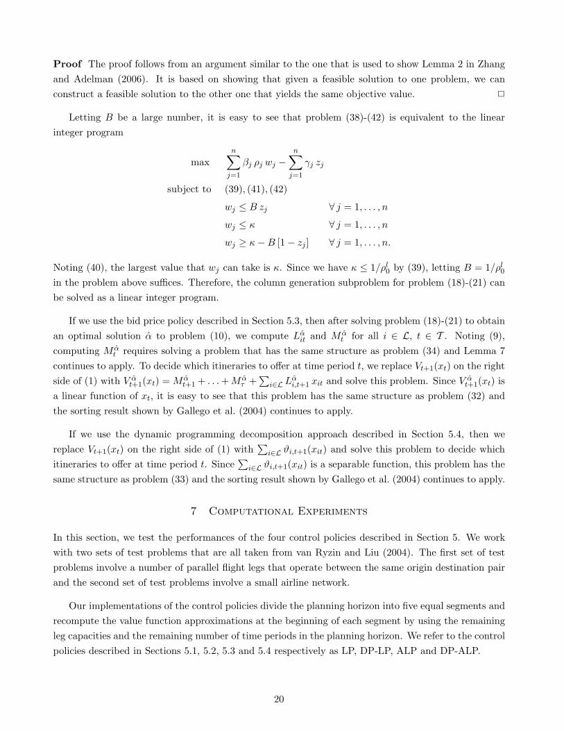
In this section, we test the performances of the four control policies described in Section 5. We workwith two sets of test problems that are all taken from van Ryzin and Liu (2004). The first set of testproblems involve a number of parallel flight legs that operate between the same origin destination pairand the second set of test problems involve a small airline network.
Our implementations of the control policies divide the planning horizon into five equal segments andrecompute the value function approximations at the beginning of each segment by using the remainingleg capacities and the remaining number of time periods in the planning horizon. We refer to the controlpolicies described in Sections 5.1, 5.2, 5.3 and 5.4 respectively as LP, DP-LP, ALP and DP-ALP.
20

Problem LP vs. DP-LP vs. CPU(q, ρ1
0, ρ20) LP DP-LP ALP DP-ALP ALP DP-ALP (secs.)
(0.6, 10−4, 10−4) 55,200 55,200 55,095 55,095 0.19 0.19 175(0.6, 1, 5) 53,400 53,378 53,281 53,276 0.22 0.19 126(0.6, 5, 10) 50,400 49,506 50,039 49,361 0.72 0.29 182(0.6, 10, 20) 45,138 44,628 44,990 44,298 0.33 0.74 124
(0.8, 10−4, 10−4) 67,200 67,200 67,060 67,060 0.21 0.21 156(0.8, 1, 5) 65,600 65,245 65,324 65,084 0.42 0.25 108(0.8, 5, 10) 59,446 59,239 59,251 58,639 0.33 1.02 86(0.8, 10, 20) 47,431 46,894 47,333 46,894 0.21 0.00 33
(1.0, 10−4, 10−4) 78,000 77,972 77,860 77,834 0.18 0.18 134(1.0, 1, 5) 76,000 75,599 75,721 75,441 0.37 0.21 100(1.0, 5, 10) 60,731 60,492 60,668 60,492 0.10 0.00 35(1.0, 10, 20) 47,442 47,368 47,442 47,368 0.00 0.00 25
(1.2, 10−4, 10−4) 88,800 88,467 88,611 88,341 0.21 0.14 123(1.2, 1, 5) 78,117 77,731 78,117 77,731 0.00 0.00 24(1.2, 5, 10) 61,038 60,905 61,038 60,905 0.00 0.00 25(1.2, 10, 20) 47,442 47,438 47,442 47,438 0.00 0.00 25
(1.4, 10−4, 10−4) 93,200 93,096 93,130 93,075 0.08 0.02 95(1.4, 1, 5) 78,117 78,084 78,117 78,084 0.00 0.00 25(1.4, 5, 10) 61,038 61,023 61,038 61,023 0.00 0.00 25(1.4, 10, 20) 47,442 47,442 47,442 47,442 0.00 0.00 25
Table 1: Comparison of the upper bounds obtained by the four control policies.
7.1 Test Problems with Parallel Flight Legs
We consider three flight legs that operate between the same origin destination pair. There is an expensiveand a cheap itinerary associated with each flight leg so that the number of itineraries is six. There aretwo customer types. The first customer type is interested only in the expensive itineraries, whereas thesecond customer type is interested only in the cheap itineraries. The capacities on the three flight legsare [30, 50, 40] and we scale these capacities by a scalar factor to obtain test problems with differentlevels of congestion. We also vary the preference weights associated with purchasing nothing. All otherproblem parameters are the same as those in van Ryzin and Liu (2004).
As described in Sections 2, 3, 5.2 and 5.4, we can obtain upper bounds on the optimal total expectedrevenue by using LP, DP-LP, ALP and DP-ALP. Table 1 shows the upper bounds obtained by thefour control policies for different test problems. In this table, the first column shows the problemcharacteristics by using the triplet (q, ρ1
0, ρ20), where q is the factor that we use to scale the leg capacities,
and ρ10 and ρ2
0 are the preference weights associated with purchasing nothing for the two customer types.The second, third, fourth and fifth columns respectively show the upper bounds obtained by LP, DP-LP,ALP and DP-ALP. The sixth column shows the percent gap between the upper bounds obtained by LPand ALP, whereas the seventh columns shows the percent gap between the upper bounds obtained byDP-LP and DP-ALP. The last column shows the CPU seconds required to solve problem (18)-(21) ona Pentium IV desktop PC with 2.4 GHz CPU and 1 GB RAM running Windows XP.
Although both LP and ALP provide upper bounds on the optimal total expected revenue, theexamples in Section 4 show that neither of these upper bounds is provably tighter than the other one.On the other hand, the empirical results in Table 1 indicate that the upper bounds obtained by ALP
21
Problem LP vs. DP-LP vs.(q, ρ1
0, ρ20) LP DP-LP ALP DP-ALP ALP DP-ALP
(0.6, 10−4, 10−4) 52,529 52,587 52,733 52,770 0.39 0.35(0.6, 1, 5) 48,836 52,315 51,720 52,593 5.58 0.53(0.6, 5, 10) 42,366 48,756 47,794 48,879 11.36 0.25(0.6, 10, 20) 37,282 43,106 42,426 43,341 12.12 0.54
(0.8, 10−4, 10−4) 63,225 63,163 63,322 63,360 0.15 0.31(0.8, 1, 5) 59,544 64,094 63,340 64,111 5.99 0.03(0.8, 5, 10) 49,706 57,568 56,478 57,658 11.99 0.16(0.8, 10, 20) 40,599 46,553 40,919 46,566 0.78 0.03
(1.0, 10−4, 10−4) 73,925 75,443 75,202 75,478 1.70 0.05(1.0, 1, 5) 65,428 74,137 71,704 74,095 8.75 -0.06(1.0, 5, 10) 54,026 60,535 55,753 60,539 3.10 0.01(1.0, 10, 20) 42,554 47,136 43,747 47,136 2.73 0.00
(1.2, 10−4, 10−4) 82,191 85,563 84,300 86,130 2.50 0.66(1.2, 1, 5) 72,921 77,823 74,591 77,842 2.24 0.02(1.2, 5, 10) 56,010 60,982 58,103 60,982 3.60 0.00(1.2, 10, 20) 43,438 47,275 45,639 47,275 4.82 0.00
(1.4, 10−4, 10−4) 86,373 89,088 86,851 89,182 0.55 0.11(1.4, 1, 5) 75,899 78,252 77,189 78,252 1.67 0.00(1.4, 5, 10) 57,470 61,220 59,819 61,220 3.93 0.00(1.4, 10, 20) 43,923 47,278 45,436 47,278 3.33 0.00
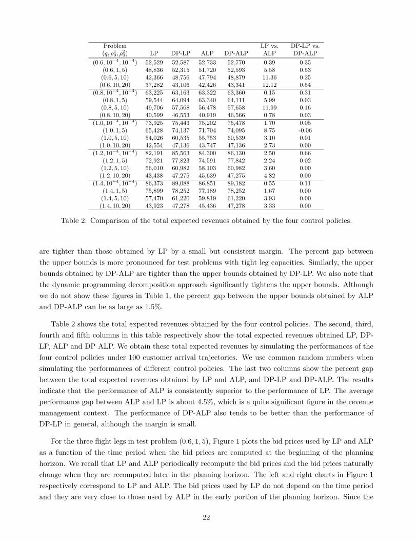
Table 2: Comparison of the total expected revenues obtained by the four control policies.
are tighter than those obtained by LP by a small but consistent margin. The percent gap betweenthe upper bounds is more pronounced for test problems with tight leg capacities. Similarly, the upperbounds obtained by DP-ALP are tighter than the upper bounds obtained by DP-LP. We also note thatthe dynamic programming decomposition approach significantly tightens the upper bounds. Althoughwe do not show these figures in Table 1, the percent gap between the upper bounds obtained by ALPand DP-ALP can be as large as 1.5%.
Table 2 shows the total expected revenues obtained by the four control policies. The second, third,fourth and fifth columns in this table respectively show the total expected revenues obtained LP, DP-LP, ALP and DP-ALP. We obtain these total expected revenues by simulating the performances of thefour control policies under 100 customer arrival trajectories. We use common random numbers whensimulating the performances of different control policies. The last two columns show the percent gapbetween the total expected revenues obtained by LP and ALP, and DP-LP and DP-ALP. The resultsindicate that the performance of ALP is consistently superior to the performance of LP. The averageperformance gap between ALP and LP is about 4.5%, which is a quite significant figure in the revenuemanagement context. The performance of DP-ALP also tends to be better than the performance ofDP-LP in general, although the margin is small.
For the three flight legs in test problem (0.6, 1, 5), Figure 1 plots the bid prices used by LP and ALPas a function of the time period when the bid prices are computed at the beginning of the planninghorizon. We recall that LP and ALP periodically recompute the bid prices and the bid prices naturallychange when they are recomputed later in the planning horizon. The left and right charts in Figure 1respectively correspond to LP and ALP. The bid prices used by LP do not depend on the time periodand they are very close to those used by ALP in the early portion of the planning horizon. Since the
22

0
300
600
900
1
250
255
260
265
270
275
280
285
290
295
300
time period
bid
pric
e
leg 1leg 2leg 3
0
300
600
900
1
250
255
260
265
270
275
280
285
290
295
300
time period
bid
pric
e
Figure 1: Bid prices used by LP and ALP as a function of the time period for test problem (0.6, 1, 5).We note that the time periods in the charts are compressed in the early portion of the planning horizon.
A H
B
C
Figure 2: Structure of the airline network.
capacities are abundant in the early portion of the planning horizon, the bid prices used by ALP tendto be constant during this period. However, as expected, the bid prices used by ALP decrease as thedeparture time approaches and fewer opportunities to utilize the leg capacities remain.
7.2 Test Problems with an Airline Network
In this set of test problems, we consider a small airline network that connects three spokes and a hub.There are 7 flight legs, 22 itineraries and 10 customer types. Half of the itineraries are expensive and theother half are cheap. Correspondingly, half of the customer types are interested only in the expensiveitineraries and the other half are interested only in the cheap itineraries. The structure of the airlinenetwork is shown in Figure 2. All problem parameters are the same as those in van Ryzin and Liu(2004) except for the number of time periods in the planning horizon and the leg capacities. We setτ = 300 and use the leg capacities shown in Table 3. Similar to Section 7.1, we obtain different testproblems by scaling the leg capacities by a scalar factor and varying the preference weights associatedwith purchasing nothing. We label our test problems by using the triplet (q, ρE
0 , ρC0 ), where q is the
scaling factor for the leg capacities, and ρE0 and ρC
0 are the preference weights associated with purchasingnothing for the customer types that are interested in the expensive and cheap itineraries.
Table 4 shows the upper bounds on the optimal total expected revenues, whereas Table 5 shows thetotal expected revenues obtained by the four control policies. The results essentially display the same
23

Flight Leg Origin Destination Capacity
1 AB 302 AH 453 AH 454 HB 455 HB 456 HC 247 HC 24
Table 3: Leg capacities for the test problems with an airline network.
Problem LP vs. DP-LP vs. CPU(q, ρE
0 , ρC0 ) LP DP-LP ALP DP-ALP ALP DP-ALP (secs.)
(0.6, 10−4, 10−4) 55,800 55,738 55,597 55,537 0.37 0.36 1,540(0.6, 1, 5) 54,430 54,201 54,097 53,942 0.62 0.48 3,065(0.6, 5, 10) 49,775 49,447 49,382 49,216 0.80 0.47 2,132(0.6, 10, 20) 44,939 44,441 44,525 44,237 0.93 0.46 2,237
(0.8, 10−4, 10−4) 68,100 67,546 67,753 67,347 0.51 0.30 1,080(0.8, 1, 5) 64,819 64,447 64,523 64,301 0.46 0.23 1,085(0.8, 5, 10) 58,350 58,065 58,010 57,881 0.59 0.32 1,167(0.8, 10, 20) 49,668 49,570 49,546 49,446 0.25 0.25 891
(1.0, 10−4, 10−4) 76,800 76,606 76,589 76,506 0.28 0.13 701(1.0, 1, 5) 73,233 72,955 72,944 72,813 0.40 0.20 859(1.0, 5, 10) 64,150 64,011 64,044 63,904 0.17 0.17 494(1.0, 10, 20) 51,321 51,125 51,321 51,125 0.00 0.00 115
(1.2, 10−4, 10−4) 85,200 85,036 84,989 84,935 0.25 0.12 585(1.2, 1, 5) 80,229 79,778 79,991 79,686 0.30 0.12 331(1.2, 5, 10) 65,321 65,212 65,321 65,212 0.00 0.00 114(1.2, 10, 20) 51,321 51,308 51,321 51,308 0.00 0.00 114
(1.4, 10−4, 10−4) 92,700 92,549 92,528 92,477 0.19 0.08 431(1.4, 1, 5) 80,876 80,825 80,876 80,825 0.00 0.00 115(1.4, 5, 10) 65,321 65,314 65,321 65,314 0.00 0.00 114(1.4, 10, 20) 51,321 51,321 51,321 51,321 0.00 0.00 114
Table 4: Comparison of the upper bounds obtained by the four control policies.
trends as those in Tables 1 and 2. For problems with tight leg capacities, the upper bounds obtainedby ALP and DP-ALP are respectively tighter than the upper bounds obtained by LP and DP-LP. Asthe leg capacities get larger, the percent gaps between the upper bounds diminish. Comparing the totalexpected revenues obtained by the different control policies, the performance gap between ALP and LPcan be as high as 4.1%. Furthermore, DP-ALP tends to perform better than DP-LP by a small butconsistent margin in general.
8 Conclusions
We presented a new deterministic linear program for the network revenue management problem withcustomer choice behavior. The novel aspect of our linear program is that it naturally generates bid pricesthat depend on the number of time periods left until the departure time. Our linear program inheritsmany features of the earlier linear program used by van Ryzin and Liu (2004). In particular, it providesan upper bound on the optimal total expected revenue, it allows using the dynamic programming
24

Problem LP vs. DP-LP vs.(q, ρE
0 , ρC0 ) LP DP-LP ALP DP-ALP ALP DP-ALP
(0.6, 10−4, 10−4) 50,187 52,239 52,350 52,871 4.13 1.20(0.6, 1, 5) 51,100 52,924 51,522 53,029 0.82 0.20(0.6, 5, 10) 46,198 48,307 46,728 48,338 1.13 0.06(0.6, 10, 20) 40,552 43,379 41,886 43,283 3.18 -0.22
(0.8, 10−4, 10−4) 61,853 64,884 63,053 65,659 1.90 1.18(0.8, 1, 5) 60,913 63,576 61,188 63,573 0.45 0.00(0.8, 5, 10) 55,098 57,003 55,670 57,074 1.03 0.12(0.8, 10, 20) 46,299 48,749 46,883 48,832 1.25 0.17
(1.0, 10−4, 10−4) 71,680 74,142 72,176 75,375 0.69 1.64(1.0, 1, 5) 70,511 72,145 70,911 72,167 0.56 0.03(1.0, 5, 10) 61,265 63,095 61,537 63,158 0.44 0.10(1.0, 10, 20) 50,486 51,057 50,583 51,049 0.19 -0.02
(1.2, 10−4, 10−4) 82,147 83,178 82,343 84,211 0.24 1.23(1.2, 1, 5) 77,220 78,952 77,918 79,098 0.90 0.18(1.2, 5, 10) 64,310 65,288 64,464 65,258 0.24 -0.05(1.2, 10, 20) 51,527 51,567 51,527 51,567 0.00 0.00
(1.4, 10−4, 10−4) 90,815 91,490 90,759 91,586 -0.06 0.10(1.4, 1, 5) 79,895 81,116 80,183 81,130 0.36 0.02(1.4, 5, 10) 65,331 65,531 65,383 65,531 0.08 0.00(1.4, 10, 20) 51,650 51,650 51,650 51,650 0.00 0.00
Table 5: Comparison of the total expected revenues obtained by the four control policies.
decomposition approach and the percent gap between its optimal objective value and the optimal totalexpected revenue diminishes as the leg capacities and the number of time periods in the planning horizonincrease linearly with the same rate. Computational experiments indicate that our linear program canprovide tighter upper bounds and the control policies that are based on our linear program can obtainhigher total expected revenues.
Unfortunately, the advantages come at a cost. In particular, the number of constraints in our linearprogram is significantly larger than the number of constraints in the linear program that appears inthe existing literature. Nevertheless, the size of our linear program is still within the capabilities of theexisting computing technology. It may also be possible to aggregate some of the constraints in problem(18)-(21) to obtain linear programs that are weaker than the linear program that we propose in thispaper, but still stronger than the earlier linear program used by van Ryzin and Liu (2004). This is anavenue of research worth pursuing.
We emphasize that the method that we use to construct our linear program can be of interest inand of itself. The idea of relaxing certain constraints in a dynamic program by associating Lagrangemultipliers with them and finding a good set of values for the Lagrange multipliers by minimizing adual function may find applications in many different problem settings. For example, Kunnumkal andTopaloglu (2006) present an application in an inventory distribution setting.
Acknowledgements
The authors acknowledge the suggestions of the associate editor and three anonymous referees. Theauthors were supported in part by the National Science Foundation grant DMI-0422133.
25
References
Belobaba, P. P. (1987), Air Travel Demand and Airline Seat Inventory Control, PhD thesis, MIT,Cambridge, MA.
Belobaba, P. P. and Weatherford, L. R. (1996), ‘Comparing decision rules that incorporate customerdiversion in perishable asset revenue management situations’, Decision Sciences 27, 343–363.
Bront, J. J. M., Mendez-Diaz, I. and Vulcano, G. (2007), A column generation algorithm for choice-basednetwork revenue management, Technical report, New York University, Stern School of Business.
Gallego, G., Iyengar, G., Phillips, R. and Dubey, A. (2004), Managing flexible products on a network,CORC Technical Report TR-2004-01, Columbia University.
Kunnumkal, S. and Topaloglu, H. (2006), An alternative to Clark and Scarf’s balance assumption forinventory distribution systems, Technical report, Cornell University, School of Operations Researchand Industrial Engineering.Available at http://legacy.orie.cornell.edu/∼huseyin/publications/publications.html.
Talluri, K. and van Ryzin, G. (1998), ‘An analysis of bid-price controls for network revenue management’,Management Science 44(11), 1577–1593.
Talluri, K. and van Ryzin, G. (2004), ‘Revenue management under a general discrete choice model ofconsumer behavior’, Management Science 50(1), 15–33.
Topaloglu, H. and Kunnumkal, S. (2006), Computing time-dependent bid-prices in network revenuemanagement problems, Technical report, Cornell University, School of Operations Research and In-dustrial Engineering.Available at http://legacy.orie.cornell.edu/∼huseyin/publications/publications.html.
van Ryzin, G. and Liu, Q. (2004), On the choice-based linear programming model for network revenuemanagement, Technical Report DRO-2004-04, Columbia Business School.
van Ryzin, G. and Vulcano, G. (2004), Computing virtual nesting controls for network revenue manage-ment under customer choice behavior, Technical Report DRO-2004-09, Columbia Business School.
Zhang, D. and Adelman, D. (2006), An approximate dynamic programming approach to network revenuemanagement with customer choice, Technical report, University of Chicago, Graduate School ofBusiness.
Zhang, D. and Cooper, W. L. (2005), ‘Revenue management for parallel flights with customer choicebehavior’, Operations Research 53(3), 415–431.
26

A Appendix: Upper Bound Obtained by the Decomposition from theDeterministic Linear Program
We let {πi : i ∈ L} be the optimal values of the dual variables associated with constraints (3) in problem(2)-(5). We choose a flight leg i and relax constraints (3) for all other flight legs by associating the dualmultipliers {πk : k ∈ L \ {i}} with them. Noting the definitions of R(S) and Qi(S), the duality theoryimplies that the linear program
ZLP = max∑
t∈T
∑
S⊂J
∑
j∈SPj(S)
[rj −
∑
k∈L\{i}akj πk
]ht(S) +
∑
k∈L\{i}πk ck
subject to (4), (5)∑
t∈T
∑
S⊂JQi(S) ht(S) ≤ ci
has the same optimal objective value as problem (2)-(5).
We consider the single-leg revenue management problem that takes place over flight leg i under theassumption that rj −
∑k∈L\{i} akj πk is the revenue associated with itinerary j. If we compare the
last problem above with problem (2)-(5) and ignore the constant term∑
k∈L\{i} πk ck in the objectivefunction, then it is easy to see that the last problem above is the linear program for the single-leg revenuemanagement problem that takes place over flight leg i. Therefore, ZLP −
∑k∈L\{i} πk ck is an upper
bound on the optimal total expected revenue for this single-leg revenue management problem. On theother hand, we can obtain the optimal total expected revenue for the single-leg revenue managementproblem that takes place over flight leg i by solving the optimality equation in (29). Therefore, wehave vi1(ci) ≤ ZLP − ∑
k∈L\{i} πk ck. This result is shown by Zhang and Adelman (2006), but ourinterpretation by using a relaxation of problem (2)-(5) appears to be new and it clearly shows why weassociate the revenue rj −
∑k∈L\{i} akj πk with itinerary j.
B Appendix: Manipulating the Objective Function of Problem (18)-(21)after Relaxing Constraints (19)
Interchanging the order of the summations, we have
∑
k∈L\{i}
∑
j∈J
∑
S⊂J
∑
t∈Tαkjt Qk(S)
[y1(S) + . . . + yt−1(S)
]
=∑
k∈L\{i}
∑
j∈J
∑
S⊂J
∑
t∈T
[αkj,t+1 + . . . + αkjτ
]Qk(S) yt(S)
=∑
t∈T
∑
S⊂J
∑
k∈L\{i}Lα
k,t+1 Qk(S) yt(S) =∑
t∈T
∑
S⊂J
∑
j∈S
∑
k∈L\{i}Pj(S) akj Lα
k,t+1 yt(S),
where the second equality follows from the definition of Lαit and the third equality follows from the
definition of Qi(S). On the other hand, the definition of Lαit implies that
∑
k∈L\{i}
∑
t∈T
∑
j∈Jαkjt ck =
∑
k∈L\{i}Lα
k1 ck.
27

Therefore, the expression∑
t∈T
∑
S⊂JR(S) yt(S)−
∑
t∈T
∑
j∈J
∑
k∈L\{i}αkjt
[ ∑
S⊂JQk(S) y1(S) + . . . +
∑
S⊂JQk(S) yt−1(S)
+∑
S⊂J1(j ∈ S) akj yt(S)− ck
]
can be written as
∑
t∈T
∑
S⊂J
∑
j∈SPj(S) rj yt(S)−
∑
t∈T
∑
S⊂J
∑
j∈S
∑
k∈L\{i}Pj(S) akj Lα
k,t+1 yt(S)
−∑
t∈T
∑
S⊂J
∑
j∈S
∑
k∈L\{i}αkjt 1(j ∈ S) akj yt(S) +
∑
k∈L\{i}Lα
k1 ck.
C Appendix: An Alternative Proof for the Sorting Result Shown byGallego et al. (2004)
In problem (32), we can immediately set zj to zero when aij > xit for some i ∈ L and we have zj ∈ {0, 1}when aij ≤ xit for all i ∈ L. Therefore, the problem inside the summation on the right side of (32) isof the form
maxz∈{0,1}n
{ ∑nj=1 βj ρj zj∑n
m=1 ρm zm + ρl0
}(43)
for appropriately defined values of n and {βj : j = 1, . . . , n}. The next proposition shows that problem(43) can be solved through a sorting procedure.
Proposition 8 Consider problem (43) and assume without loss of generality that β1 ≥ β2 ≥ . . . ≥ βn.There exists an optimal solution z = {zj : j = 1, . . . , n} to this problem that satisfies
zj =
{1 if j < K
0 if j ≥ K(44)
for an appropriately defined value of K ∈ {1, . . . , n + 1}.
Proof As a function of ε, we let g(ε) be the optimal objective value of the linear program
max1
ε + ρl0
n∑
j=1
βj ρj zj (45)
subject ton∑
j=1
ρj zj = ε (46)
0 ≤ zj ≤ 1 ∀ j = 1, . . . , n. (47)
It is easy to see that g(ε) is a continuous function of ε over the interval [0,∑n
j=1 ρj ] and the optimalobjective value of the problem maxε∈[0,
Pnj=1 ρj ]{g(ε)} is equal to the optimal objective value of the
28
continuous relaxation of problem (43). We show the final result in two steps. The first step shows thatif ε =
∑K−1j=1 ρj for some K ∈ {1, . . . , n + 1}, then there exists an optimal solution to problem (45)-(47)
that has the same form as (44). The second step shows that there exists an optimal solution ε to theproblem maxε∈[0,
Pnj=1 ρj ]{g(ε)} that satisfies ε =
∑K−1j=1 ρj for some K ∈ {1, . . . , n+1}. These two steps
show that the continuous relaxation of problem (43) has an integer optimal solution and this solutionhas the same form as (44).
The first step immediately follows from the fact that problem (45)-(47) is a continuous knapsackproblem and an optimal solution can be found by sorting the items according to their utility to spaceratios. For the second step, it is enough to show that the derivative of g(·) does not change sign overthe interval (
∑K−1j=1 ρj ,
∑Kj=1 ρj) for all K ∈ {1, . . . , n}. We note that if ε ∈ (
∑K−1j=1 ρj ,
∑Kj=1 ρj), then
an optimal solution to problem (45)-(47) can be obtained by letting zj = 1 for all j = 1, . . . , K − 1,zK = ε/ρK −∑K−1
j=1 ρj/ρK and zj = 0 for all j = K + 1, . . . , n. Therefore, we have
g(ε) =1
ε + ρl0
{K−1∑
j=1
βj ρj + βK
[ε−
K−1∑
j=1
ρj
]}.
The derivative of g(·) is
1[ε + ρl
0
]2
{βK ρl
0 −K−1∑
k=1
βj ρj + βK
K−1∑
j=1
ρj
}
and its sign does not depend on the value of ε. 2
Therefore, we can find an optimal solution to problem (43) by sorting {βj : j = 1, . . . , n} andchecking n + 1 possible solutions. The values of {ρj : j = 1, . . . , n} do not play a role in the sortingprocedure and our proof clearly shows why this is the case.
29