a resample-based sva algorithm for sidelobe …core.ecu.edu/geog/wangy/papers_in_pdfs/2015_a...

1016 IEEE TRANSACTIONS ON GEOSCIENCE AND REMOTE SENSING, VOL. 53, NO. 2, FEBRUARY 2015

A Resample-Based SVA Algorithm for SidelobeReduction of SAR/ISAR Imagery With

Noninteger Nyquist Sampling RateTao Xiong, Associate Member, IEEE, Shuang Wang, Biao Hou, Member, IEEE, Yong Wang, and Hongying Liu

Abstract—A resample-based spatial variant apodization (SVA)algorithm for sidelobe reduction was studied for synthetic aper-ture radar (SAR) and inverse SAR (ISAR) imagery with a noninte-ger Nyquist sampling rate. The weighting function of every samplein the image domain was calculated with the sample and two ad-jacent noninteger samples. The noninteger samples were obtainedby interpolation in the image domain using sinc function. Withthe proper selection of two noninteger samples, the monotonicproperty of the weighting function on each side of the samplingpoint was preserved. The unequivocal determination of sidelobesuppression was achieved for noninteger Nyquist sampled (NINS)SAR and ISAR imagery. In addition, the lower and upper bound-aries of the weighting function under the cosine-on-pedestal con-dition were extended for further sidelobe suppression and mainlobe sharpening. The algorithm was implemented and applied toNINS imagery that is simulated. The algorithm was then assessedfor acquired SAR and ISAR images. Improved results have beenqualitatively and quantitatively achieved in sidelobe suppressionand main lobe sharping in comparison with an existing algorithm.

Index Terms—Inverse synthetic aperture radar (ISAR), nonin-teger Nyquist sampled (NINS) imagery, SAR, sidelobe reductionalgorithm.

I. INTRODUCTION

THE quality of high-resolution synthetic aperture radar(SAR) and inverse SAR (ISAR) [1]–[7] images may be

negatively affected when radar signals are collected from anarea where numerous targets of strong radar return exist. Thetargets, for example, can be corner reflectors formed by build-ings and streets, as well as metallic objects such as air condi-tioning units on rooftops and vehicles on surface roads in urbanarea. The targets are not only of strong main lobes but also ofhigh sidelobes in radar returns. Visually, they are no longerany points on an image. Instead, they are brightand starlike

Manuscript received August 30, 2013; revised March 8, 2014; acceptedMay 7, 2014. This work was supported in part by Xidian University underGrant JB140230 and Grant K5051399058 and in part by the Program forCheung Kong Scholars and Innovative Research Team in University underGrant IRT1170.

T. Xiong, S. Wang, and B. Hou are with the Key Laboratory of IntelligentPerception and Image Understanding of the Ministry of Education, Interna-tional Research Center for Intelligent Perception and Computation, XidianUniversity, Xi’an 710071, China (e-mail: [email protected]).

Y. Wang is with the Department of Geography, Planning and Environment,East Carolina University, Greenville, NC 27858 USA.

H. Liu with the School of Electronic Engineering and the Key Laboratory ofIntelligent Perception and Image Understanding of the Ministry of Education,Xidian University, Xi’an 710071, China.

Digital Object Identifier 10.1109/TGRS.2014.2332252

crosses. In such cases, linear segments off the cross centerscould overlap or shadow other targets, particularly weak targetsspatially. Therefore, the entire imagery might be degradedbecause of the negative influence of the sidelobes of the strongtargets. Sidelobe at low levels or sidelobe reduction is explicitlyrequired in the application of SAR and ISAR imagery.

There are two types of widely used methods to reducesidelobes. One is the linear technique and is applied in thefrequency domain before a final formation of a SAR or anISAR image [1], [2]. With weights in the frequency domainsuch as Hanning and Hamming weights, the sidelobes can besuppressed to a very low level. Unfortunately, due to a constantweight used, the main lobe is usually widened. The imageresolution becomes coarse [1]. Thus, the linear technique maynot applicable for high-resolution imaging. The other is thenonlinear technique that is typically called as the spatial variantapodization (SVA) [8]–[16]. Of the SVA technique, differentweighting functions for individual samples of the SAR or ISARimage are generated in the image domain. For each sample, theweight is calculated from the values of the sample itself andof two adjacent sample points. Under the cosine-on-pedestalcondition, the lower and upper limits of the weighting functionare typically from 0 to 1/2 [8]. The output is obtained fromthe combination of weight and three samples. The SVA of [8]is developed for integer Nyquist sampled (INS) SAR or ISARdata. Satisfactory results in sidelobe suppression are obtainedin image processing of INS data. The algorithm [8] becomesa benchmark in sidelobe suppression (for INS radar imagery)because numerous derivative algorithms are studied [10]–[12]and all are assessed by the algorithm [8]. To increase theapplicability of the INS SVA algorithm, Smith [13] successfullyextends the algorithm to process noninteger Nyquist sampled(NINS) SAR or ISAR image. Promising results in sidelobesuppression have been achieved for most of the NINS images.Since then, Smith’s algorithm [13] becomes a representative forthe NINS SVA algorithm, and is widely used in the processingof NINS images. Several derivatives from Smith’s algorithmare developed [14]–[16]. However, as one closely examinesimagery output from Smith’s algorithm, some sidelobe effectscould not be minimized.

Analytically, the success of sidelobe suppression in INSSAR and ISAR data using the INS SVA algorithms [8]–[12] isattributed to the weighting function that is monotonic on eitherside of a sample point. In other words, the monotonic attributeof the two-side function helps unequivocally determine whether

0196-2892 © 2014 IEEE. Personal use is permitted, but republication/redistribution requires IEEE permission.See http://www.ieee.org/publications_standards/publications/rights/index.html for more information.

XIONG et al.: SVA FOR SIDELOBE REDUCTION OF SAR/ISAR IMAGERY WITH NYQUIST SAMPLING RATE 1017

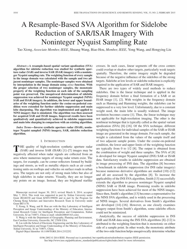
Fig. 1. (a) Impulse response of I(n). (b) Weighting function for one target.

sidelobe suppression is needed or not. Unfortunately, after theextension of the INS SVA algorithms [8]–[12] to the NINS SVAones [13]–[16], the monotonic feature is not preserved. Thus,the unequivocal determination of sidelobe suppression cannotbe accomplished for NINS SAR or ISAR data. Sidelobes atunacceptably high level could remain. The quality of SAR andISAR data can be adversely affected. Therefore, the impetusis to develop a NINS SVA algorithm in which the monotonicproperty of weighting function should not be altered. Indeed,the property is kept in the proposed resample-based NINS SVAalgorithm that consists of the following major steps. First, twovalues of adjacent noninteger samples of each related sampleare selected and calculated using sinc interpolation. Then, theweight function for the sample is derived through minimization.Next, ranges of lower and upper limits of the weighting functionare studied and expanded with the understanding of their rolesplayed in suppressing sidelobes and sharpening main lobes.Then, the algorithm is implemented and applied in analyses ofsimulated and acquired SAR and ISAR data. Finally, in the per-formance assessment of the algorithm, benchmark algorithmsof the INS SVA [8] and the NINS SVA [13] are implemented aswell. Results from three algorithms are evaluated.

II. SVA ALGORITHM

A. Algorithm for INS SAR and ISAR Images

For simplicity, the SVA [8] is discussed along 1-D data ofone Nyquist sampled SAR/ISAR image. Let gSVA(n) be the nthsample of complex value of one row data after the processingof SVA with N elements or pixels and gSVA(n) = ISVA(n) +jQSVA(n). ISVA(n) and QSVA(n) are the real and imaginarycomponents of gSVA(n), respectively. One way to reduce side-lobes is to minimize ISVA(n) and QSVA(n) separately [8]. Asan example, the output of the real part can be written as

ISVA(n) = I(n) + w(n) [I(n− 1) + I(n+ 1)] (1)

where I(n) is the input of the real part. Therefore, the aim is tofind w(n) such that |ISVA(n)|2 is minimized. Mathematically,with d|ISVA(n)|2/dw(n) = 0, w(n) is solved as

w(n) = − I(n)

I(n− 1) + I(n+ 1). (2)

Then, the output of the real part is [8]

ISVA(n)=

⎧⎨⎩

I(n), w(n) < 00, 0 ≤ w(n) ≤ 1

2I(n)+ 1

2 [I(n−1)+I(n+ 1)] , w(n) > 12 .

(3)

(It should be noted that QSVA(n) output of the imaginary partcan be similarly obtained.)

In the image domain, the discussed SVA can be understoodusing an INS sinc function. Under the INS case or one Nyquistsampled case as the simplest example, a single sinc function isinitially considered. If there is only one target in the scene, I(n)can be expressed as

I(n) = sinc(n− n0) =sin π(n− n0)

π(n− n0). (4)

In addition

sin π(n− n0 ± 1) = − sin π(n− n0). (5)

Substituting (4) into (2), one obtains

w(n) =− I(n)

I(n− 1) + I(n+ 1)

=− sinc(n− n0)

sinc(n−1−n0)+sinc(n+1−n0)=

(n−n0)2−1

2(n− n0)2.

(6)

Graphically, the impulse response and the weighting functionunder the INS from one target are illustrated (see Fig. 1).Clearly, on either side of n− n0, I(n) and w(n) are monotonic.When |n− n0| ≤ 1, the sample is within the interval of themain lobe [see Fig. 1(a)] [8] and w(n) ≤ 0 [see Fig. 1(b)].Hence, with ISVA(n) = I(n) in (3), the main lobe is notwidened. When |n− n0| > 1, 0 ≤ w(n) ≤ 1/2 [see Fig. 1(b)].Thus, the sample falls inside sidelobes [see Fig. 1(a)]. LetISVA(n) = 0; therefore, the sidelobes are removed. From (6),one also has {

limn−n0→+∞

w(n) = 12

w(n)|n−n0=±1 = 0.(7)

Thus, w(n) cannot be greater than 1/2 when there is a singletarget. In the case of multiple targets, w(n) may be greater than1/2. The SVA still works, and the sidelobes are reduced to avery low level [8].


Fig. 2. (a) Impulse response of I(n). Weighting function for one target under a NINS case. Ws = 0.67.

B. Algorithm for NINS SAR and ISAR Images

The SVA can suppress sidelobes well for the INS case [8],[9]. However, the algorithm might not be able to suppress thesidelobes completely under the NINS case although there isonly one single sinc function. Under such case, the real partof the signal is

I(n) = sinc [Ws(n− n0)] =sin πWs(n− n0)

πWs(n− n0)(8)

with 0 < Ws < 1. In (8), 1/Ws is the noninteger Nyquistsampling rate and is also called as the oversampling ratio [20].Therefore

sin πWs(n− n0 ± 1) = sin [πWs(n− n0)± πWs]

�= − sin [πWs(n− n0)] . (9)

Similar to (2), the weighting function can be computed as

w(n)

=− I(n)

I(n−1)+I(n+1)

=− sinc [Ws(n−n0)]

sinc [Ws(n−n0−1)]+sinc [Ws(n−n0+1)]

=−[(n−n0)

2−1]tanπ[Ws(n−n0)]

2(n−n0)2tanπ[Ws(n−n0)]cosπWs−2(n−n0)sinπWs.

(10)

Equivalently to Fig. 1, I(n)(8) and w(n) (10) are illustratedin Fig. 2. Different from the INS case, I(n) and w(n) are notmonotonic on either side of n− n0 [see Fig. 2(a) cf., Fig. 1(a);and Fig. 2(b) cf., Fig. 1(b)]. In the example, the main lobecan be preserved without widening using (1)–(3). However,the sidelobes may not be suppressed because some samplessuch as P at (nx − n0)can be located inside the sidelobes [seeFig. 2(a)] and their related w(n) is less than zero. Therefore,when w(n) < 0 [see the first condition in (3)], ISVA(n) =I(n). Values related to the sidelobes are unchanged, or thereduction of sidelobes is not done.

III. RESAMPLE-BASED SVA ALGORITHM

UNDER NINS CONDITION

The monotonic property of w(n) is not held for a NINSSAR image as discussed above. Therefore, a new algorithm is

proposed in which the weighting function is monotonic at eitherside of the sample point, and the algorithm should be applicableto the NINS case.

A. Derivation for the Resample-Based SVA Algorithm

Let n be the sample of interest. (n− 1/Ws) and (n+ 1/Ws)are two adjacent noninteger sample locations of n. Mathemat-ically, the values of noninteger samples at (n− 1/Ws) and(n+ 1/Ws) for the single sinc function are{

I(n− 1/Ws) =sin[πWs(n−n0−1/Ws)]

πWs(n−n0−1/Ws)

I(n+ 1/Ws) =sin[πWs(n−n0+1/Ws)]

πWs(n−n0+1/Ws).

(11)

To be concise, we only present one sinc function in thederivation. The developed algorithm works for multiple sincfunctions, as shown in the analyses of simulated and acquiredSAR and ISAR data. Numerators on the right side of (11) canbe simplified as

sin [πWs(n− n0 ± 1/Ws)] = sin [πWs(n− n0)± π]

= −sin [πWs(n−n0)] . (12)

At sample locations (n− 1/Ws) and (n+ 1/Ws), clearly,(12) is equivalent to (5). Similar to the SVA, w(n) in theproposed SVA algorithm is

w(n) = − I(n)

I(n− 1/Ws) + I(n+ 1/Ws)

= −sin πWs(n−n0)πWs(n−n0)

− sin πWs(n−n0)π[Ws(n−n0)−1] + − sin πWs(n−n0)

π[Ws(n−n0)+1]

=W 2

s (n− n0)2 − 1

2W 2s (n− n0)2

. (13)

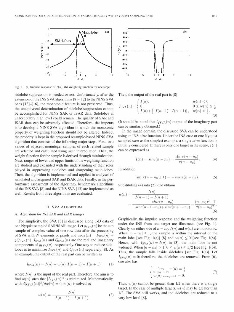
As shown in Fig. 3, w(n) is monotonic in either left or rightside of n− n0. In short, (13) is very similar to the weightfunction in the INS case (6). The monotonic feature of theweighting function is preserved.

B. Resampling Operation for the Proposed SVA Algorithm

Since values of I(n− 1/Ws) and I(n+ 1/Ws) cannot beobtained directly from radar signal parameters of SAR or ISAR,


Fig. 3. Weight function for the proposed resample-based SVA algorithm.

a resampling or an interpolation operation is alternatively used.Interpolation can be implemented using convolution [1]⎧⎪⎪⎨

⎪⎪⎩I(n− 1/Ws) =

+∞∑p=−∞

[I(n− p)δ(−1/Ws − p)]

I(n+ 1/Ws) =+∞∑

p=−∞[I(n− p)δ(1/Ws − p)]

(14)

where δ(·) is an interpolation function [1]. Although manyinterpolation (e.g., polynomial and cubic spline) functions exist[17], [18], a special and widely used interpolation function fora radar signal [1] is used. The function is based on a sincfunction. In particular, if a radar signal is sampled at discreteand evenly spaced intervals, the signal can be reconstructedwithout loss or error if the following conditions of Nyquist’ssampling theorem are met [1].

• The signal is band limited.• The sampling satisfies Nyquist’s sampling rule.A sinc function

δ(n) = sinc(n) =sin(πn)

πn(15)

for the SAR or ISAR system always meets above two condi-tions. In addition, as a tradeoff between accuracy and computa-tional efficiency, (14) is often approximated as [1], [2]⎧⎪⎪⎪⎨⎪⎪⎪⎩

I(n− 1/Ws) ≈P∑

p=−P

[I(n− p)sinc(−1/Ws − p)]

I(n+ 1/Ws) ≈P∑

p=−P

[I(n− p)sinc(1/Ws − p)]

(16)

and only (2P + 1) samples are used to calculate I(n− 1/Ws)and I(n+ 1/Ws), respectively. Then, w(n) is derived as

w(n) = − I(n)

I(n− 1/Ws) + I(n− 1/Ws). (17)

Furthermore, two parameters, i.e., γmin and γmax (see Fig. 3),are introduced to help expand the range of cosine-on-pedestalcondition. The output of the real part IRSVA(n) is exampled as

IRSVA(n)

=

⎧⎪⎨⎪⎩I(n), w(n)<γmin

0, γmin≤w(n)≤γmax

I(n)+γmax [I(n−1/Ws)+ I(n+1/Ws)] , w(n)>γmax.

(18)

The imaginary part QRSVA(n) can be obtained in the same way.Therefore, the output using the resample-based SVA algorithmunder the NINS condition is obtained.

When γmin = 0 and γmax = 1/2, the range for the weightingfunction is the same as that of the weight function in [8]. Asshown in Fig. 3, γmin is set to be less than zero. A negativeγmin helps sharpen the main lobe because at the edge of themain lobe and with (13), one has

w(n) =W 2

s (n− n0)2 − 1

2W 2s (n− n0)2

= γmin. (19)

Solving (n− n0), one obtains

n− n0 = ± 1

Ws

√1− 2γmin

. (20)

The width of the main lobe after the proposed algorithm is

L=1

Ws

√1−2γmin

−(− 1

Ws

√1−2γmin

)=

2

Ws

√1−2γmin

.

(21)

L decreases as γmin varies from 0 to a negative value. Thus,the main lobe is narrowed, or the resolution of the image isimproved. Theoretically, the smaller the value of γmin is, thehigher the resolution of the image could be. However, whenγmin becomes too small, some energy within the main lobefrom a target can be lost. As a result, the signal from the mainlobe can be low. The signal-to-noise ratio is adversely impacted.

If w(n) > γmax, γmax is used to replace w(n) in (18). Asobserved in the analysis of simulated and acquired images,w(n) > γmax occurs when multiple targets in the same sceneexist. In such cases, a target or targets with the weak radarreturns are covered by echoes of the sidelobes from one ormultiple strong radar targets. The real part of the sample is

I(n) =

R∑r=1

δrsinc [Ws(n− nr)] +N(n)

=

R∑r=1

δrsin πWs(n− nr)

πWs(n− nr)+N(n) (22)

where there are R targets in the scene. δr and nr are themagnitude and location for each target; N(n) is the possibleunsystemic error. The output becomes

IRSVA(n) = I(n) + γmax [I(n− 1/Ws) + I(n+ 1/Ws)]

=R∑

r=1

δrsinc [Ws(n− nr)] +N(n)

+ γmax

[R∑

r=1

δrsinc [Ws(n− nr − 1/Ws)]

+

R∑r=1

δrsinc [Ws(n− nr + 1/Ws)]

+N(n− 1/Ws) +N(n+ 1/Ws)

]

=

R∑r=1

δr

⟨sinc [Ws(n− nr)]

+1

2{sinc [Ws(n− nr − 1/Ws)]

+sinc [Ws(n− nr + 1/Ws)]}⟩

+ΔE(n) (23)


with

ΔE(n) =

(γmax −

1

2

){R∑

r=1

δrsinc [Ws(n− nr − 1)]

+R∑

r=1

δrsinc [Ws(n− nr + 1)]

}

+

(γmax−

1

2

)[N(n−1)+N(n+1)]+N(n). (24)

In addition

sinc [Ws(n− nr)] +1

2{sinc [Ws(n− nr − 1/Ws)]

+ sinc [Ws(n− nr + 1/Ws)]}

=sin πWs(n− nr)

πWs(n− nr)+

1

2

[sin πWs(n− nr − 1/Ws)

πWs(n− nr − 1/Ws)

+sin πWs(n− nr + 1/Ws)

πWs(n− nr + 1/Ws)

]

=sin πWs(n− nr)

πWs(n− nr)− 1

2

sin πWs(n− nr)

πWs

×[

1

(n− nr − 1/Ws)+

1

(n− nr + 1/Ws)

]

=sin πWs(n− nr)

πWs(n− nr)

1/W 2s

(n− nr)2 − 1/W 2s

. (25)

With substitution of (25) into (23), the output of the real part is

IRSVA(n)=R∑

r=1

δrsinc [Ws(n− nr)]

W 2s [(n− nr)2−1/W 2

s ]+ΔE(n). (26)

From (26), one also has (27), shown at the bottom of thepage. Therefore, the output of (26) consists of two parts. In thefirst part, the impulse response becomes sinc[Ws(n− nr)]/[(n− nr)

2 − 1/W 2s ]. The magnitude is nearly unchanged

when n− nr → 0. Most of the main lobes are preserved.When n− nr is far away from zero, the related magnitude israpidly decreasing by dividing (n− nr)

2 − 1/W 2s . Thus, the

sidelobes are suppressed. The second term in (26) is relatedto the noise of I(n− 1/Ws), I(n), and I(n+ 1/Ws). Withappropriate selection of γmax, the term can be minimized orthe noise decreases to some extent. Unfortunately, the optimalparameter cannot be analytically obtained. Furthermore, energyfrom scatterers within the scene could be severely suppressed orbecome undetectable when γmax is too large.

C. Implementation and Assessment of an Image Before andAfter Processing

The resample-based SVA algorithm is implemented along therange direction first and then the azimuth direction. In addition,in the assessment of image quality after this algorithm, animage contrast is used. It is defined as

C =1

αmax

αmax∑α=1

σα

μα(28)

with⎧⎪⎪⎪⎪⎨⎪⎪⎪⎪⎩

μα = 1βmax

βmax∑β=1

gnormalized(α, β)

σα =

√√√√ 1βmax

[βmax∑β=1

(gnormalized(α, β)− μα)2

] (29)

where g(α, β) is the image of the number of rows αmax and thenumber of columns βmax. 1 ≤ α ≤ αmax and 1 ≤ β ≤ βmax.gnormalized(α, β) is |g(α, β)| after normalization. Normaliza-tion is needed in order to intercompare among the input imageand output images from this algorithm and others used incomparison. Finally, the higher the contrast value is, the betterthe image quality is quantitatively.

IV. RESULTS

A. Analysis of Simulated Data

The proposed algorithm was first assessed using simulated1-D SAR data [real part, Fig. 4(a)]. The expression of thedata was ⎧⎨

⎩I(n) = I1(n) + I2(n)I1(n) = sinc [Ws(n− n1)]I2(n) = a · sinc [Ws(n− n2)]

(30)

where −8 ≤ n ≤ 8, Ws = 0.67, n1 = 2.35, n2 = 4.85, anda = 1.56. There were two targets of strong radar return or twoNINS sinc functions I1(n) and I2(n). They were located atn1 = 2.35 and n2 = 4.85, individually. The width of each mainlobe was 1.5 sample widths. Due to the sidelobe interferenceamong targets, the main lobe of the first strong target was nowcentered at n1 = 2.00, and the main lobe of the second strongtarget at n2 = 5.00. Thus, two centers were 3.00 samples apart.Peaks of sinc functions, as circled in Fig. 4(a), representedintensities of two main lobes, respectively. The main lobesmight overlap that could lead to the ambiguity of two targets.

⎧⎪⎪⎪⎪⎪⎪⎪⎪⎨⎪⎪⎪⎪⎪⎪⎪⎪⎩

limn−nr→1/Ws

sinc [Ws(n− nr)]

(n− nr)2 − 1/W 2s

= limn−nr→1/Ws

− sin [πWs(n− nr − 1/Ws)]

[πWs(n− nr)] [(n− nr)− 1/Ws] [(n− nr) + 1/Ws]

= limn−nr→1/Ws

−1

(n− nr) [(n− nr) + 1/Ws]= −W 2

s

2

limn−nr→0

sinc [Ws(n− nr)]

W 2s · [(n− nr)2 − 1/W 2

s ]= − 1

(27)


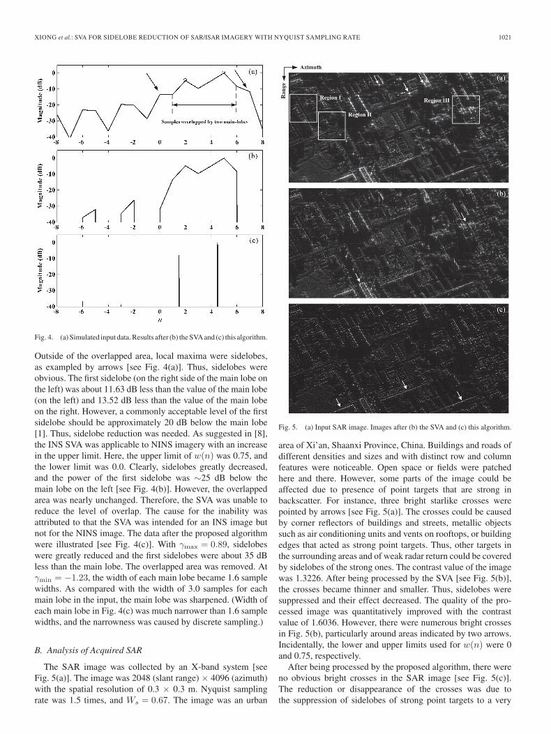
Fig. 4. (a) Simulated input data. Results after (b) the SVA and (c) this algorithm.

Outside of the overlapped area, local maxima were sidelobes,as exampled by arrows [see Fig. 4(a)]. Thus, sidelobes wereobvious. The first sidelobe (on the right side of the main lobe onthe left) was about 11.63 dB less than the value of the main lobe(on the left) and 13.52 dB less than the value of the main lobeon the right. However, a commonly acceptable level of the firstsidelobe should be approximately 20 dB below the main lobe[1]. Thus, sidelobe reduction was needed. As suggested in [8],the INS SVA was applicable to NINS imagery with an increasein the upper limit. Here, the upper limit of w(n) was 0.75, andthe lower limit was 0.0. Clearly, sidelobes greatly decreased,and the power of the first sidelobe was ∼25 dB below themain lobe on the left [see Fig. 4(b)]. However, the overlappedarea was nearly unchanged. Therefore, the SVA was unable toreduce the level of overlap. The cause for the inability wasattributed to that the SVA was intended for an INS image butnot for the NINS image. The data after the proposed algorithmwere illustrated [see Fig. 4(c)]. With γmax = 0.89, sidelobeswere greatly reduced and the first sidelobes were about 35 dBless than the main lobe. The overlapped area was removed. Atγmin = −1.23, the width of each main lobe became 1.6 samplewidths. As compared with the width of 3.0 samples for eachmain lobe in the input, the main lobe was sharpened. (Width ofeach main lobe in Fig. 4(c) was much narrower than 1.6 samplewidths, and the narrowness was caused by discrete sampling.)

B. Analysis of Acquired SAR

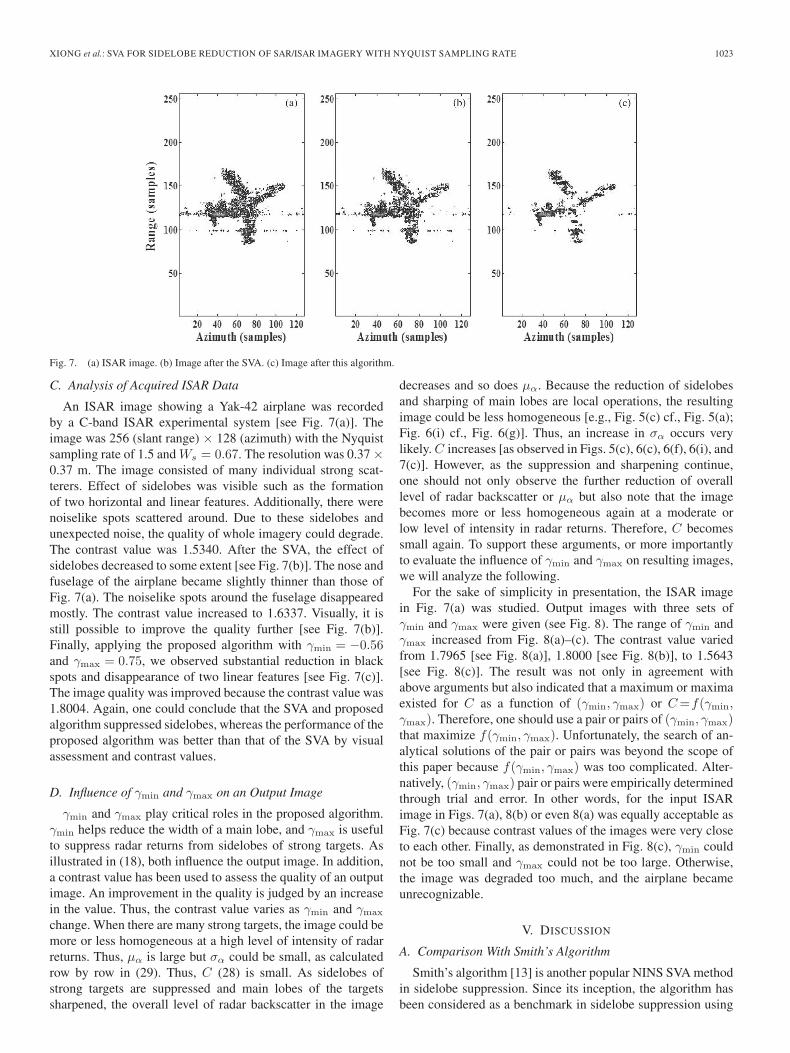
The SAR image was collected by an X-band system [seeFig. 5(a)]. The image was 2048 (slant range) × 4096 (azimuth)with the spatial resolution of 0.3 × 0.3 m. Nyquist samplingrate was 1.5 times, and Ws = 0.67. The image was an urban

Fig. 5. (a) Input SAR image. Images after (b) the SVA and (c) this algorithm.

area of Xi’an, Shaanxi Province, China. Buildings and roads ofdifferent densities and sizes and with distinct row and columnfeatures were noticeable. Open space or fields were patchedhere and there. However, some parts of the image could beaffected due to presence of point targets that are strong inbackscatter. For instance, three bright starlike crosses werepointed by arrows [see Fig. 5(a)]. The crosses could be causedby corner reflectors of buildings and streets, metallic objectssuch as air conditioning units and vents on rooftops, or buildingedges that acted as strong point targets. Thus, other targets inthe surrounding areas and of weak radar return could be coveredby sidelobes of the strong ones. The contrast value of the imagewas 1.3226. After being processed by the SVA [see Fig. 5(b)],the crosses became thinner and smaller. Thus, sidelobes weresuppressed and their effect decreased. The quality of the pro-cessed image was quantitatively improved with the contrastvalue of 1.6036. However, there were numerous bright crossesin Fig. 5(b), particularly around areas indicated by two arrows.Incidentally, the lower and upper limits used for w(n) were 0and 0.75, respectively.

After being processed by the proposed algorithm, there wereno obvious bright crosses in the SAR image [see Fig. 5(c)].The reduction or disappearance of the crosses was due tothe suppression of sidelobes of strong point targets to a very


Fig. 6. Close-view images of three regions (by row). By column, SAR images as input, images after the SVA, and images after the proposed algorithm.

low level. Furthermore, metallic edges of buildings becamenarrower (as exampled by three arrows) in Fig. 5(c) than thosein Fig. 5(a) or (b). The contrast value was 3.2572. It shouldbe noted that γmin = −1.23 and γmax = 0.89 were used. Aspreviously discussed, the lower limit less than 0 and the upperlimit greater than 0.75 for w(n) could not only further suppresssidelobes but could also sharpen main lobes. Because of thesharping in main lobes and sidelobe suppression, the equivalentsignal strength in Fig. 5(c) decreased. Thus, Fig. 5(c) lookedvisually darker than Fig. 5(a) or (b). In short, there should bea tradeoff of image quality measured by the signal-to-noiseratio, as well as the sharping of main lobes and suppressionof sidelobes. Therefore, γmin should not be too small, and γmax

should not be too big. The determinations of both parameterswere further studied later.

To further discuss the performance of the proposed algo-rithm, three small areas were identified as regions I, II, andIII [see Fig. 5(a)]. Each region is 512 (slant range) × 512(azimuth). In Region I, there was nearly lack of targets (orscatterers) that are of strong radar returns. Thus, effects fromsidelobes of the strong targets could be minimal. No brightcrosses were obviously noted in Fig. 6(a)–(c). Their contrastvalues were given in Table I. Thus, the quality of images afterthe SVA and proposed algorithm was improved due to theincrease in contrast values. In Region II, there was an increasein the number of strong targets shown as bright crosses [seeFig. 6(d)]. Most strong targets were far apart spatially except fortwo clusters (of strong ones). Although some crosses were con-verted as bright spots using the SVA, there were several crossesremained [see Fig. 6(e)]. Thus, the effectiveness of the SVA in

TABLE ICONTRAST VALUES OF IMAGES IN THREE REGIONS

sidelobe suppression decreased. After being processed by theproposed algorithm, all the crosses were nearly converted asbright spots [see Fig. 6(f)]. As quantified by contrast values (seeTable I), the proposed algorithm performed the best in sidelobesuppression in Region II. Finally, there were significantly morestrong scatterers or targets in Region III [see Fig. 6(g)], as com-pared with those in Region I [see Fig. 6(a)] and Region II [seeFig. 6(d)]. In addition, the targets were clustered and overlappedby each other [see Fig. 6(g)]. Areas of targets that are of lowradar returns were severely contaminated by sidelobes of strongtargets. The contrast value was 1.1005 (see Table I). Fig. 6(h)was processed with the SVA. A majority of all crosses existedand were scattered around the image although the contrast valueincreased (see Table I). Thus, one could argue that the SVAdid not suppress sidelobes well. Finally, using the proposedalgorithm, there was significant reduction in the number ofcrosses [see Fig. 6(i)]. The contrast value became 2.9028 (seeTable I). In summary, the proposed algorithm and SVA wereable to suppress sidelobes of strong targets and to increasecontrast values. The proposed algorithm outperformed the SVA.


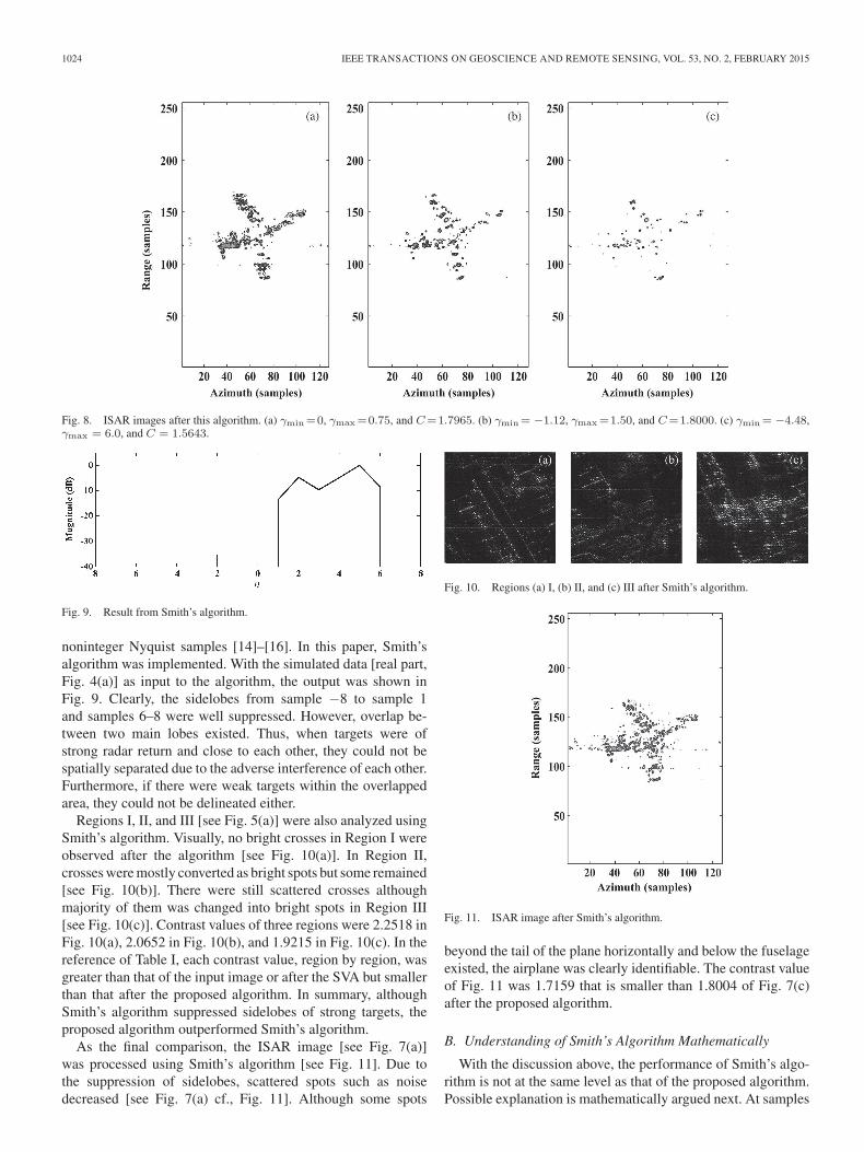
Fig. 7. (a) ISAR image. (b) Image after the SVA. (c) Image after this algorithm.

C. Analysis of Acquired ISAR Data

An ISAR image showing a Yak-42 airplane was recordedby a C-band ISAR experimental system [see Fig. 7(a)]. Theimage was 256 (slant range) × 128 (azimuth) with the Nyquistsampling rate of 1.5 and Ws = 0.67. The resolution was 0.37 ×0.37 m. The image consisted of many individual strong scat-terers. Effect of sidelobes was visible such as the formationof two horizontal and linear features. Additionally, there werenoiselike spots scattered around. Due to these sidelobes andunexpected noise, the quality of whole imagery could degrade.The contrast value was 1.5340. After the SVA, the effect ofsidelobes decreased to some extent [see Fig. 7(b)]. The nose andfuselage of the airplane became slightly thinner than those ofFig. 7(a). The noiselike spots around the fuselage disappearedmostly. The contrast value increased to 1.6337. Visually, it isstill possible to improve the quality further [see Fig. 7(b)].Finally, applying the proposed algorithm with γmin = −0.56and γmax = 0.75, we observed substantial reduction in blackspots and disappearance of two linear features [see Fig. 7(c)].The image quality was improved because the contrast value was1.8004. Again, one could conclude that the SVA and proposedalgorithm suppressed sidelobes, whereas the performance of theproposed algorithm was better than that of the SVA by visualassessment and contrast values.

D. Influence of γmin and γmax on an Output Image

γmin and γmax play critical roles in the proposed algorithm.γmin helps reduce the width of a main lobe, and γmax is usefulto suppress radar returns from sidelobes of strong targets. Asillustrated in (18), both influence the output image. In addition,a contrast value has been used to assess the quality of an outputimage. An improvement in the quality is judged by an increasein the value. Thus, the contrast value varies as γmin and γmax

change. When there are many strong targets, the image could bemore or less homogeneous at a high level of intensity of radarreturns. Thus, μα is large but σα could be small, as calculatedrow by row in (29). Thus, C (28) is small. As sidelobes ofstrong targets are suppressed and main lobes of the targetssharpened, the overall level of radar backscatter in the image

decreases and so does μα. Because the reduction of sidelobesand sharping of main lobes are local operations, the resultingimage could be less homogeneous [e.g., Fig. 5(c) cf., Fig. 5(a);Fig. 6(i) cf., Fig. 6(g)]. Thus, an increase in σα occurs verylikely. C increases [as observed in Figs. 5(c), 6(c), 6(f), 6(i), and7(c)]. However, as the suppression and sharpening continue,one should not only observe the further reduction of overalllevel of radar backscatter or μα but also note that the imagebecomes more or less homogeneous again at a moderate orlow level of intensity in radar returns. Therefore, C becomessmall again. To support these arguments, or more importantlyto evaluate the influence of γmin and γmax on resulting images,we will analyze the following.

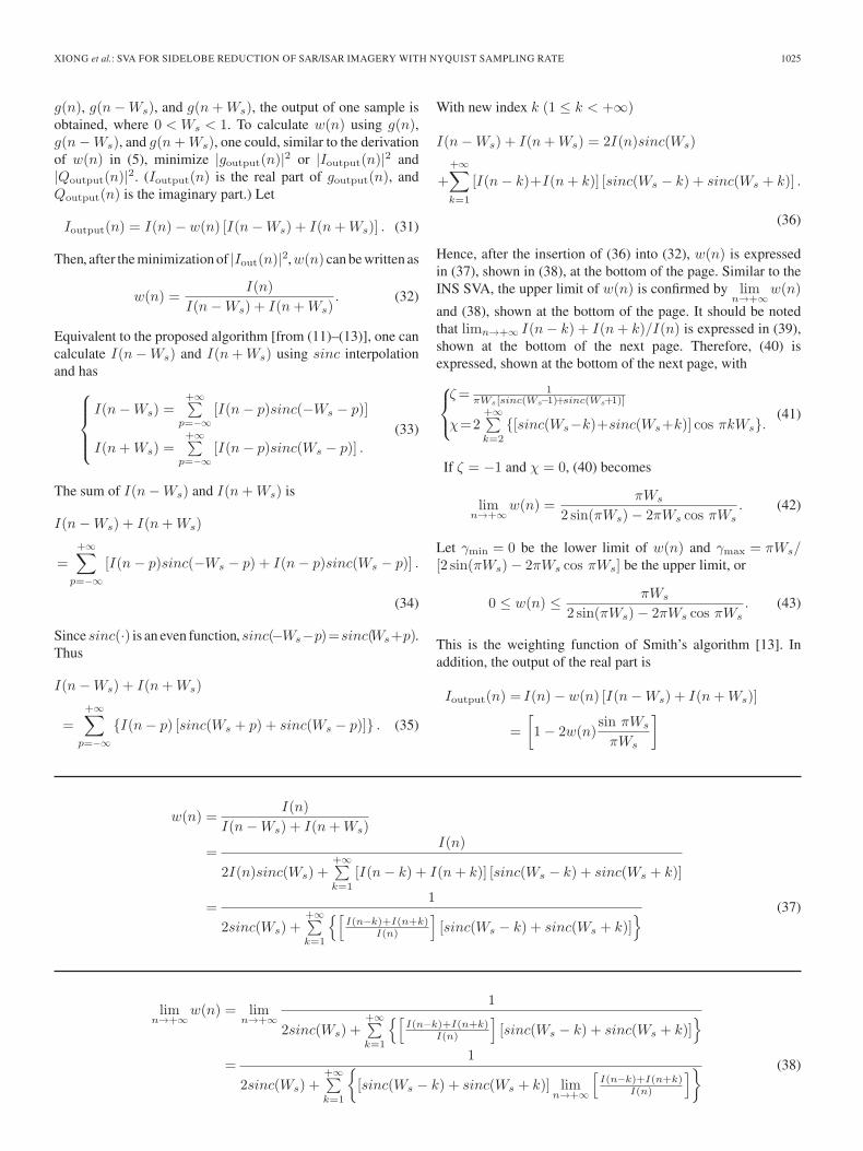
For the sake of simplicity in presentation, the ISAR imagein Fig. 7(a) was studied. Output images with three sets ofγmin and γmax were given (see Fig. 8). The range of γmin andγmax increased from Fig. 8(a)–(c). The contrast value variedfrom 1.7965 [see Fig. 8(a)], 1.8000 [see Fig. 8(b)], to 1.5643[see Fig. 8(c)]. The result was not only in agreement withabove arguments but also indicated that a maximum or maximaexisted for C as a function of (γmin, γmax) or C=f(γmin,γmax). Therefore, one should use a pair or pairs of (γmin, γmax)that maximize f(γmin, γmax). Unfortunately, the search of an-alytical solutions of the pair or pairs was beyond the scope ofthis paper because f(γmin, γmax) was too complicated. Alter-natively, (γmin, γmax) pair or pairs were empirically determinedthrough trial and error. In other words, for the input ISARimage in Figs. 7(a), 8(b) or even 8(a) was equally acceptable asFig. 7(c) because contrast values of the images were very closeto each other. Finally, as demonstrated in Fig. 8(c), γmin couldnot be too small and γmax could not be too large. Otherwise,the image was degraded too much, and the airplane becameunrecognizable.

V. DISCUSSION

A. Comparison With Smith’s Algorithm

Smith’s algorithm [13] is another popular NINS SVA methodin sidelobe suppression. Since its inception, the algorithm hasbeen considered as a benchmark in sidelobe suppression using


Fig. 8. ISAR images after this algorithm. (a) γmin=0, γmax=0.75, and C=1.7965. (b) γmin= −1.12, γmax=1.50, and C=1.8000. (c) γmin= −4.48,γmax = 6.0, and C = 1.5643.

Fig. 9. Result from Smith’s algorithm.

noninteger Nyquist samples [14]–[16]. In this paper, Smith’salgorithm was implemented. With the simulated data [real part,Fig. 4(a)] as input to the algorithm, the output was shown inFig. 9. Clearly, the sidelobes from sample −8 to sample 1and samples 6–8 were well suppressed. However, overlap be-tween two main lobes existed. Thus, when targets were ofstrong radar return and close to each other, they could not bespatially separated due to the adverse interference of each other.Furthermore, if there were weak targets within the overlappedarea, they could not be delineated either.

Regions I, II, and III [see Fig. 5(a)] were also analyzed usingSmith’s algorithm. Visually, no bright crosses in Region I wereobserved after the algorithm [see Fig. 10(a)]. In Region II,crosses were mostly converted as bright spots but some remained[see Fig. 10(b)]. There were still scattered crosses althoughmajority of them was changed into bright spots in Region III[see Fig. 10(c)]. Contrast values of three regions were 2.2518 inFig. 10(a), 2.0652 in Fig. 10(b), and 1.9215 in Fig. 10(c). In thereference of Table I, each contrast value, region by region, wasgreater than that of the input image or after the SVA but smallerthan that after the proposed algorithm. In summary, althoughSmith’s algorithm suppressed sidelobes of strong targets, theproposed algorithm outperformed Smith’s algorithm.

As the final comparison, the ISAR image [see Fig. 7(a)]was processed using Smith’s algorithm [see Fig. 11]. Due tothe suppression of sidelobes, scattered spots such as noisedecreased [see Fig. 7(a) cf., Fig. 11]. Although some spots

Fig. 10. Regions (a) I, (b) II, and (c) III after Smith’s algorithm.

Fig. 11. ISAR image after Smith’s algorithm.

beyond the tail of the plane horizontally and below the fuselageexisted, the airplane was clearly identifiable. The contrast valueof Fig. 11 was 1.7159 that is smaller than 1.8004 of Fig. 7(c)after the proposed algorithm.

B. Understanding of Smith’s Algorithm Mathematically

With the discussion above, the performance of Smith’s algo-rithm is not at the same level as that of the proposed algorithm.Possible explanation is mathematically argued next. At samples


g(n), g(n−Ws), and g(n+Ws), the output of one sample isobtained, where 0 < Ws < 1. To calculate w(n) using g(n),g(n−Ws), and g(n+Ws), one could, similar to the derivationof w(n) in (5), minimize |goutput(n)|2 or |Ioutput(n)|2 and|Qoutput(n)|2. (Ioutput(n) is the real part of goutput(n), andQoutput(n) is the imaginary part.) Let

Ioutput(n) = I(n)− w(n) [I(n−Ws) + I(n+Ws)] . (31)

Then, after the minimization of |Iout(n)|2,w(n) can be written as

w(n) =I(n)

I(n−Ws) + I(n+Ws). (32)

Equivalent to the proposed algorithm [from (11)–(13)], one cancalculate I(n−Ws) and I(n+Ws) using sinc interpolationand has⎧⎪⎪⎨

⎪⎪⎩I(n−Ws) =

+∞∑p=−∞

[I(n− p)sinc(−Ws − p)]

I(n+Ws) =+∞∑

p=−∞[I(n− p)sinc(Ws − p)] .

(33)

The sum of I(n−Ws) and I(n+Ws) is

I(n−Ws) + I(n+Ws)

=

+∞∑p=−∞

[I(n− p)sinc(−Ws − p) + I(n− p)sinc(Ws − p)] .

(34)

Since sinc(·) is an even function, sinc(−Ws−p)=sinc(Ws+p).Thus

I(n−Ws) + I(n+Ws)

=

+∞∑p=−∞

{I(n− p) [sinc(Ws + p) + sinc(Ws − p)]} . (35)

With new index k (1 ≤ k < +∞)

I(n−Ws) + I(n+Ws) = 2I(n)sinc(Ws)

+

+∞∑k=1

[I(n− k)+I(n+ k)] [sinc(Ws − k) + sinc(Ws + k)] .

(36)

Hence, after the insertion of (36) into (32), w(n) is expressedin (37), shown in (38), at the bottom of the page. Similar to theINS SVA, the upper limit of w(n) is confirmed by lim

n→+∞w(n)

and (38), shown at the bottom of the page. It should be notedthat limn→+∞ I(n− k) + I(n+ k)/I(n) is expressed in (39),shown at the bottom of the next page. Therefore, (40) isexpressed, shown at the bottom of the next page, with⎧⎨⎩ζ= 1

πWs[sinc(Ws−1)+sinc(Ws+1)]

χ=2+∞∑k=2

{[sinc(Ws−k)+sinc(Ws+k)] cos πkWs}.(41)

If ζ = −1 and χ = 0, (40) becomes

limn→+∞

w(n) =πWs

2 sin(πWs)− 2πWs cos πWs. (42)

Let γmin = 0 be the lower limit of w(n) and γmax = πWs/[2 sin(πWs)− 2πWs cos πWs] be the upper limit, or

0 ≤ w(n) ≤ πWs

2 sin(πWs)− 2πWs cos πWs. (43)

This is the weighting function of Smith’s algorithm [13]. Inaddition, the output of the real part is

Ioutput(n) = I(n)− w(n) [I(n−Ws) + I(n+Ws)]

=

[1− 2w(n)

sin πWs

πWs

]

w(n) =I(n)

I(n−Ws) + I(n+Ws)

=I(n)

2I(n)sinc(Ws) ++∞∑k=1

[I(n− k) + I(n+ k)] [sinc(Ws − k) + sinc(Ws + k)]

=1

2sinc(Ws) ++∞∑k=1

{[I(n−k)+I(n+k)

I(n)

][sinc(Ws − k) + sinc(Ws + k)]

} (37)

limn→+∞

w(n) = limn→+∞

1


{[I(n−k)+I(n+k)

I(n)

][sinc(Ws − k) + sinc(Ws + k)]

}=

1


{[sinc(Ws − k) + sinc(Ws + k)] lim

n→+∞

[I(n−k)+I(n+k)

I(n)

]} (38)


× I(n)− w(n)+∞∑k=1

[I(n− k) + I(n+ k)]

× [sinc(Ws − k) + sinc(Ws + k)]

=

[1− 2w(n)

sin πWs

πWs

]

× I(n)− κw(n) [I(n− 1) + I(n+ 1)] + Δε

(44)

with {κ = sinc(Ws − 1) + sinc(Ws + 1)Δε = −χw(n)/2.

(45)

If κ = −1 and Δε = 0, (44) is simplified as

Ioutput(n) =

[1− 2w(n)

sin πWs

πWs

]I(n)

+ w(n) [I(n− 1) + I(n+ 1)] . (46)

This is Smith’s algorithm [13]. Thus, extending the derivationscheme in the development of the proposed algorithm forsidelobe suppression, we have shown that Smith’s algorithmcan be derived as a special case here. Because ζ = −1, χ = 0,κ = −1, and Δε = 0 cannot be always valid at locations wheremultiple strong targets are highly and locally concentrated[e.g., Fig. 7(g)], some sidelobes that are at unacceptably highlevel of intensity could still exist after Smith’s algorithm. Theinvalidation was attributed as one of possible causes of thedeficiency in Smith’s algorithm.

C. Comparison With Two Other Approaches

In addition to Smith’s method, Castillo-Rubio et al. [19]and Yocky et al. [20] proposed two modified NINS SVAs tosuppress sidelobes. The output of the real part of the method ofCastillo-Rubio et al. was

IC(m,n)= aWsmWsnI(m,n)

+ wmWsmWsn [I(m− 1, n) + I(m+ 1, n)]

+ wmmWsmWsn [I(m− 2, n) + I(m+ 2, n)]

+ wnWsmWsn [I(m,n− 1) + I(m,n+ 1)]

+ wnnWsmWsn [I(m,n− 2) + I(m,n+ 2)]

+ wmnWsmWsn

∑p={−1,1}q={−1,1}

[I(m+p,n)+I(m,n+q)]

(47)

with

a=1−2wmsinc(Wsm)−2wmmsinc(2Wsm)−2wnsinc(Wsn)

−2wnnsinc(2Wsn)− 4wmnsinc(Wsm)sinc(Wsn) (48)

where m and p are indices in the m-direction, and n and qare in the n-direction of an image. Wsm and Wsn are knownconstants. wm, wn, wmn, wnn, and wmm are weights unknown.Five weights are solved using a linear function in a 5-D spacesuch that IC(m,n) is minimized [19]. This method could be gen-erally interpreted as an extension of Smith’s method from 1-Dinto 2-D. In [20], the output of the real part as an example was

IY (m,n) = I(m,n) + wmQm + wnQn + wmwnP (49)

with (50), shown at the bottom of the page. Qm, Qn, and P areobtained by interpolation. wm is within interval [0, 1/2], and sois wn. Together, the intervals form a square with four corners

limn→+∞

I(n− k) + I(n+ k)

I(n)= lim

n→+∞

sin πWs(n−n0−k)πWs(n−n0−k) + sin πWs(n−n0+k)

πWs(n−n0+k)

sin πWs(n−n0)πWs(n−n0)

= limn→+∞

2(n− n0)2 sin πWs(n− n0) cos πkWs − 2(n− n0) cos πWs(n− n0) sin πkWs

[(n− n0)2 − 1] sin πWs(n− n0)= 2 cos πkWs (39)

limn→+∞

w(n) =1

2sinc(Ws) + 2+∞∑k=1

{[sinc(Ws − k) + sinc(Ws + k)] · cos πkWs}

=πWs

2 sin(πWs) + 2ζπWs cos(πWs) + χ(40)

⎧⎪⎨⎪⎩

Qm = I(m− 1/Wsm, n) + I(m+ 1/Wsm, n)Qn = I(m,n− 1/Wsn) + I(m,n+ 1/Wsn)P = I(m− 1/Wsm, n− 1/Wsn) + I(m+ 1/Wsm, n− 1/Wsn)

+I(m− 1/Wsm, n+ 1/Wsn) + I(m+ 1/Wsm, n+ 1/Wsn)

(50)


of (0,0), (1/2,0), (1/2,1/2), and (0,1/2). To minimize IY (m,n),Yocky et al. calculate IY (m,n) at four corners. If one of thefour IY (m,n)’s has the opposite sign with that of I(m,n),IY (m,n) is set to zero. For all IY (m,n)’s of the same sign(positive or negative), the one of the smallest absolute value ischosen as the output. Thus, the sidelobe is suppressed. Differentfrom Smith’s algorithm and ours, two 2-D filters are used [19],[20]. As Stankwitz et al. [8] previously stated, the 1-D approachwas fast in sidelobe suppression (in comparison with a 2-Dapproach in general).

VI. CONCLUSION

A novel SVA algorithm to handle INS SAR and ISAR imageshas been studied. With the appropriate selection of two adjacentnoninteger samples, the weighting function became monotonicin both sides of the sample point or away from peak again.Whether sidelobe suppression was needed or not, it has beenunequivocally determined for NINS SAR and ISAR imagery. Inaddition, the range of lower and upper limits of the weightingfunction was expanded to suppress sidelobes and to sharpenmain lobes further. The algorithm was implemented in analysesof simulated and acquired data sets.

In simulation studies, sidelobes were well suppressed, andwidths of two main lobes narrowed after applying the proposedmethod. In addition, the overlapped area between two mainlobes was removed. Thus, the two-side monotonic feature ofthe weighting function was invaluable in sidelobe reduction forNINS imagery through resampling operation. Then, acquiredSAR and ISAR images were then processed using this algo-rithm. Overall, there was a significant reduction in sidelobesof strong targets because various bright starlike crosses wereconverted as points. The contrast value increased. To furtherassess the performance of the algorithm, we evaluated out-puts from three closed-view areas where strong radar targetschanged from a minimum number to a high number, and fromspatially apart to highly concentrate. Since sidelobes weregreatly suppressed, one actually could identify and count thenumber of bright crosses that are converted as bright points.In addition, metallic edges of buildings became narrower incomparison with those of the input image. Thus, the resultswere very promising quantitatively and quantitatively. Similarperformance in sidelobe suppression and main lobe sharpeningwas achieved in the analysis of an ISAR image showing anairplane. The nose, wings, fuselage, and tail were clearly identi-fied. As case-by-case comparisons, the proposed algorithm out-performed the INS SVA visually and quantitatively as measuredby contrast values of imagery.

As discussed, values of the lower limit γmin and upper limitγmax of the weighting function played critical role in the studiedalgorithm. The main lobe width has been analytically derivedas a function of γmin. As γmin decreases, the width decreases.Thus, γmin was invaluable in narrowing main lobe. γmax wasuseful in sidelobe reduction. Due to the complicity, the deriva-tion of the analytic relationship of the sidelobe suppressionand γmax was believed to be beyond the scope of this paper.Alternatively, pairs of (γmin, γmax) that can maximize contrastvalues were determined as empirically solutions, alternatively.

Smith’s algorithm has been popular in processing NINS im-agery. The algorithm has been implemented. Outputs from thisalgorithm and Smith’s one were assessed. Again, case by case,this algorithm outperformed Smith’s algorithm. Finally, havingdeveloped this algorithm, we proved that Smith’s algorithm wasderivable as a special case using the derivation scheme for thisalgorithm and analytically explored possible cause or causes forthe deficiency of Smith’s algorithm in processing some NINSimagery. It was attributed that if ζ = −1, χ = 0, κ = −1, andΔε = 0 were not valid simultaneously, Smith’s algorithm couldnot suppress some sidelobes to a very low level.

REFERENCES

[1] I. G. Cumming and F. H. Wong, Digital Processing of Synthetic Aper-ture Radar Data: Algorithms and Implementation. Norwood, MA, USA:Artech House, 2005.

[2] W. G. Carrara, R. S. Goodman, and R. M. Majewski, Spotlight SyntheticAperture Radar: Signal Processing Algorithm. Boston, MA: ArtechHouse, 1995.

[3] M. Soumtkh, “Reconnaissance with ultra wideband UHF synthetic aper-ture radar,” IEEE Signal Process. Mag., vol. 12, no. 4, pp. 21–40,Jul. 1995.

[4] G. C. Sun et al., “A unified focusing algorithm for several modes ofSAR based on FrFT,” IEEE Trans. Geosci. Remote Sens., vol. 51, no. 5,pp. 3139–3455, May 2013.

[5] A. Ferro, D. Brunner, and L. Bruzzone, “Automatic detection and recon-struction of building radar footprints from single VHR SAR images,”IEEE Trans. Geosci. Remote Sens., vol. 51, no. 2, pp. 935–952, Feb. 2013.

[6] B. Zhang et al., “Ocean vector winds retrieval from C-band fully polari-metric SAR measurements,” IEEE Trans. Geosci. Remote Sens., vol. 50,no. 11, pp. 4252–4261, Nov. 2012.

[7] G. O. Glentis, K. X. Zhao, A. Jakobsson, and J. Li, “Non-parametric high-resolution SAR imaging,” IEEE Trans. Signal Process., vol. 61, no. 7,pp. 1614–1624, Apr. 2013.

[8] H. C. Stankwitz, R. J. Dallaire, and J. R. Fienup, “Nonlinear apodizationfor side lobe control in SAR imagery,” IEEE Trans. Aerosp. Electron.Syst., vol. 31, no. 1, pp. 267–279, Jan. 1995.

[9] S. R. DeGraaf, “SAR imaging via modern 2-D spectral estimation meth-ods,” IEEE Trans. Image Process., vol. 7, no. 5, pp. 729–761, May 1998.

[10] C. H. Seo and J. T. Yen, “Side lobe suppression in ultrasound imagingusing dual apodization with cross-correlation,” IEEE Trans. Ultrason.,Ferroelectr., Freq. Control, vol. 55, no. 10, pp. 2498–2210, Oct. 2008.

[11] C. H. Seo and J. T. Yen, “Evaluating the robustness of dual apodiza-tion with cross-correlation,” IEEE Trans. Ultrason„ Ferroelectr., Freq.Control, vol. 56, no. 2, pp. 291–303, Feb. 2009.

[12] R. Iglesias and J. J. Mallorqui, “Side-lobe cancelation in DInSAR pixelselection with SVA,” IEEE Geosci. Remote Sens. Lett., vol. 10, no. 4,pp. 667–671, Jul. 2013.

[13] B. H. Smith, “Generalization of spatially variant apodization to noninte-ger Nyquist sampling rates,” IEEE Trans. Image Process., vol. 9, no. 6,pp. 1088–1093, Jun. 2000.

[14] X. J. Xu and R. M. Narayanan, “Enhanced resolution in SAR/ISAR imag-ing using iterative side lobe apodization,” IEEE Trans. Image Process.,vol. 14, no. 4, pp. 537–547, Apr. 2005.

[15] C. F. Castillo-Rubio, S. Llorente-Romano, and M. Burgos-García, “Spa-tially variant apodization for squinted synthetic aperture radar images,”IEEE Trans. Image Process., vol. 16, no. 8, pp. 2023–2027, Aug. 2007.

[16] B. G. Lim, J. C. Woo, and Y. S. Kim, “Noniterative super-resolutiontechnique combining SVA with modified geometric mean filter,” IEEEGeosci. Remote Sens. Lett., vol. 7, no. 4, pp. 713–717, Oct. 2010.

[17] W. H. Press, S. A. Teukolsky, W. T. Vetterling, and B. P. Flannery, Nu-merical Recipes in C: The Art of Scientific Computing. New York, NY,USA: Cambridge Univ. Press, 1992.

[18] W. Y. Yang, W. Cao, T.-S. Chung, and J. Morris, Applied NumericalMethods Using MATLAB. New York, NY, USA: Wiley, 2005.

[19] C. F. Castillo-Rubio, S. Llorente-Romano, and M. Burgos-García, “Ro-bust SVA method for every sampling rate condition,” IEEE Trans. Aerosp.Electron. Syst., vol. 43, no. 2, pp. 571–580, Apr. 2007.

[20] D. A. Yocky, C. V. Jakowats, Jr., and P. H. Eichel, “Interpolated spa-tially variant apodization in synthetic aperture radar imagery,” Appl. Opt.,vol. 39, no. 14, pp. 2310–2312, May 2000.


Tao Xiong (A’13) was born in Hubei, China, inJanuary 1984. He received the Master’s degree incontrol technology and instrument from Xidian Uni-versity, Xi’an, China, in 2006.

He is currently with the Key Laboratory of Intel-ligent Perception and Image Understanding of theMinistry of Education of China, Xidian University.His research interests include imaging of severalsynthetic aperture radar modes and autofocus.

Shuang Wang was born in Shaanxi, China, in 1978.She received the B.S. and M.S. degrees and thePh.D. degree in circuits and systems from XidianUniversity, Xi’an, China, in 2000, 2003, and 2007,respectively.

Currently, she is a Professor with the Key Lab-oratory of Intelligent Perception and Image Under-standing of the Ministry of Education of China,Xidian University. Her main research interests aresparse representation, image processing, and high-resolution synthetic aperture radar image processing.

Biao Hou (M’07) was born in China in 1974. He re-ceived the B.S. and M.S. degrees in mathematics fromNorthwest University, Xi’an, China, in 1996 and1999, respectively, and the Ph.D. degree in circuitsand systems from Xidian University, Xi’an, in 2003.

Since 2003, he has been with the Key Laboratoryof Intelligent Perception and Image Understandingof the Ministry of Education of China, Xidian Univer-sity, where he is currently a Professor. His researchinterests include multiscale geometric analysis andsynthetic aperture radar image processing.

Yong Wang received the Ph.D. degree from theUniversity of California, Santa Barbara, CA, USA,in 1992, with focus on synthetic aperture radar andits application in forested environments.

He is currently a Faculty Member with EastCarolina University, Greenville, NC, USA. His gen-eral research area is the application of remotelysensed and geospatial data sets to environments, nat-ural hazards, and air pollution and is firmly couchedwithin coastal areas of the USA.

Hongying Liu received the B.E. and M.S. degreesin computer science and technology from Xi’AnUniversity of Technology, Xi’An, China, in 2002 and2006, respectively, and the Ph.D. degree in engineer-ing from Waseda University, Tokyo, Japan, in 2012.

Currently, she is a Faculty Member with theSchool of Electronic Engineering and the Key Lab-oratory of Intelligent Perception and Image Un-derstanding of the Ministry of Education, XidianUniversity, Xi’An, China. Her major research inter-ests include intelligent signal processing, machine

learning, compressive sampling, etc.

a resample-based sva algorithm for sidelobe …core.ecu.edu/geog/wangy/papers_in_pdfs/2015_a...

Documents