a robust asset–liability management framework for
TRANSCRIPT
OR Spectrum (2016) 38:1007–1041DOI 10.1007/s00291-016-0437-z
REGULAR ARTICLE
A robust asset–liability management framework forinvestment products with guarantees
Nalan Gülpınar1 · Dessislava Pachamanova2 ·Ethem Çanakoglu3
Received: 6 September 2014 / Accepted: 12 February 2016 / Published online: 28 March 2016© The Author(s) 2016. This article is published with open access at Springerlink.com
Abstract This paper suggests a robust asset–liability management framework forinvestment products with guarantees, such as guaranteed investment contracts andequity-linked notes. Stochastic programming and robust optimization approaches areintroduced to deal with data uncertainty in asset returns and interest rates. The statisti-cal properties of the probability distributions of uncertain parameters are incorporatedin the model through appropriately selected symmetric and asymmetric uncertaintysets. Practical data-driven approaches for implementation of the robust models arealso discussed. Numerical results using generated and real market data are presentedto illustrate the performance of the robust asset–liability management strategies.The robust investment strategies show better performance in unfavorable marketregimes than traditional stochastic programming approaches. The effectiveness ofrobust investment strategies can be improved by calibrating carefully the shape andthe size of the uncertainty sets for asset returns.
Keywords Uncertainty modeling · Investment contracts with guarantees ·Asset–liability management · Robust optimization · Stochastic programming
B Nalan Gülpı[email protected]
Dessislava [email protected]
Ethem Ç[email protected]
1 Warwick Business School, The University of Warwick, Coventry CV4 7AL, UK
2 Mathematics and Sciences Division, Babson College, Wellesley, MA 02457, USA
3 Industrial Engineering Department, Bahcesehir University, Istanbul, Turkey
123

1008 N. Gulpinar et al.
1 Introduction
Investment products with guarantees offer policyholders a guaranteed stream of pay-ments and a portion of the potential gains on an underlying asset over a fixed periodof time. Examples of such products include Guaranteed Investment Contracts (GICs),issued by insurance companies, and Equity-Linked Notes (ELNs), issued by invest-ment banks. Investment products with guarantees provide a smoothing of portfolioreturns to the policy (note) holders, so that the latter do not experience the full volatil-ity of the underlying portfolio (Consiglio et al. 2006).
The basic structure of a typical GIC is as follows. The investor pays the “principal”upfront, and then receives a guaranteed rate of return over the life of the contract (Stiefel1984). The last payment includes the value of the principal. Guaranteed investmentcontracts are popular investment vehicles—AIG notoriously used US$9 billion ofthe government bailout after the crisis in the late 2000s to pay out on guaranteedinvestment contracts it had sold to investors (Walsh 2008). ELNs have similar termsto GICs. However, the payment stream is linked to the value of an equity security suchas an equity index or a portfolio of assets. A portion of the returns generated by theequity index or the portfolio of assets over a specified period is paid to the policyholder(Ramaswami et al. 2001; Miltersen and Persson 2003; Toy and Ryan 2000). Theprincipal is typically guaranteed, and hence the investor obtains fixed-income-likeprincipal protection of his investment with an equity market upside exposure (Hardy2003). At maturity, the guaranteed return and added bonuses along with the originalcapital invested are returned to the noteholder.
Firms issuing investment products with guarantees face an asset–liability man-agement (ALM) problem. On the one hand, they need to invest the available capital(assets) collected from the principal payments profitably. On the other hand, they needto manage their obligations (liabilities) to policy holders. Insurance companies issuingGICs typically take a different approach from banks issuing ELNs. The former poolthe premiums from the policy holders and invest them in a portfolio with a substantialequity component (see Consiglio et al. 2006) or a fixed income component (see Chap-ter 15 in Pachamanova and Fabozzi 2016). The latter typically hedge their exposureby purchasing exotic options or combinations of financial derivatives.
In this paper, we focus on the particular problem faced by an issuer of an invest-ment product with guarantees that would like to determine the optimal structure ofan underlying equity portfolio so as to maximize net portfolio return while meet-ing liabilities. This problem has not been addressed much in the literature. At thesame time, a substantial amount of research has been directed at solving the pric-ing problem for investment contracts with guarantees—namely, determining the bestguaranteed rate of return and optimal values for other contract features. In solvingthe pricing problem, the underlying portfolio is assumed to be given exogenouslyrather than structured optimally. For example, going as far back as the 1970s, Brennanand Schwartz (1976) determine the equilibrium pricing of equity-linked life insur-ance policies with an asset value guarantee. Brennan and Schwartz (1979) discussinvestment strategies for equity-linked life insurance policies with an asset valueguarantee. Mallier and Alobaidi (2002) develop a Vasicek model to price equity-linked notes where the holder receives both interest payments and payments linked to
123

A robust asset–liability management framework 1009
the performance of an equity index. Bacinello (2003) studies the problem of pric-ing a participating policy sold in the Italian market using guaranteed investmentcontracts. Nietert (2003) investigates option based portfolio insurance and modeluncertainty. As shown by Consiglio et al. (2001), however, firms can substantiallyincrease their profits and offer higher guarantees by investing a higher proportion oftheir assets in an optimally structured equity portfolio. Consiglio et al. (2006) applystochastic programming to find the optimal structure of the portfolio underlying aninsurance company’s fund. Consiglio et al. (2008) discuss various issues with assetand liability modeling for participating policies with guarantees. Valle et al. (2014)develop a mixed integer optimization model for a portfolio of assets that is designedto deliver a constant return per time period irrespective of how the underlying marketperforms.
We propose a robust optimization approach to structuring the optimal portfoliofor investment products with guarantees. The approach addresses two issues withpreviously suggested computational approaches to managing the underlying portfoliofor GICs and ELNs: tractability and representation of the underlying uncertainties.Whilewe are concernedwith optimal allocation, the proposed approach can potentiallyhave applications in the pricing of such contracts as well. As wementioned, the currentliterature on pricing assumes that the structure of the portfolio is given exogenously.Because this approach is computationally efficient and tractable, acceptable valuesfor the parameters of the contract can be derived by solving the optimal structuringproblemmultiple times to determine the parameters that will result in the highest profitfor the issuer of the contract.
Robust optimization was first introduced by Ben-Tal and Nemirovski (1998) andEl Ghaoui and Lebret (1997). Since then, it has been applied for solving variouspractical problems in different areas. The robust optimization approach assumes thatthe uncertain parameters in an optimization problem belong to uncertainty sets thatcan be constructed from the probability distributions of uncertain factors. A robustcounterpart of the original problem requires that the optimal solution to the opti-mization problem remain feasible for all realizations of the stochastic data within thepre-specified uncertainty sets, including the worst-case values if they can be found.Depending on the specification of the uncertainty sets, the robust counterparts of theoriginal optimization problems can be formulated as tractable optimization problemswith no random parameters. For further information on robust optimization and recentdevelopments, the reader is referred to Ben-Tal et al. (2009).
Robust optimization applications in finance have been primarily in asset man-agement (for a comprehensive overview, see Fabozzi et al. 2007). The robustmean-variance portfolio selection framework has been widely studied; see, forinstance, Goldfarb and Iyengar (2003), Gulpinar and Rustem (2007), Oguzsoy andGuven (2007), andSoyster andMurphy (2013).Robust investment strategies in amulti-period setting are studied in Ben-Tal et al. (2000) and Bertsimas and Pachamanova(2008). Pinar (2007) studies a robust scenario-optimization-based downside risk mea-sure for multi-period portfolio selection. Pae and Sabbaghi (2014) consider log-robustportfolios after transaction costs. Gulpinar and Pachamanova (2013) develop a robustALMmodel for a pension fundwith time-varying asset returns using ellipsoidal uncer-tainty sets mapped from a time series model for asset returns. The ALM model for a
123

1010 N. Gulpinar et al.
typical pension fund involves contributions from wages over the life of the contract,and the liabilities are paid from the fund.
This paper makes three main contributions to the literature. First, we show how themulti-period allocation problem for equity portfolios underlying investment productswith guarantees can be cast in a robust multi-period optimization framework. Sec-ond, we are able to incorporate asymmetries in the distribution of asset returns in thisframework. The latter is important for practical implementation because there is sub-stantial empirical evidence that asset returns are not symmetrically distributed (see, forexample, the discussion in Natarajan et al. 2008). Third, we suggest a scenario-baseddata-driven approach for estimating the input parameters in the robust formulations.We design numerical experiments to illustrate the performance of the robust ALMmodels under different assumptions on the behavior of the underlying uncertainties.We also compare the performance of robustALM investment strategieswith the perfor-mance of expected value optimization using generated and real market data. By takinga worst-case view, the robust optimization approach to asset-liability management ofinvestment products with guarantees allows for incorporating newways to analyze theperformance of investment policies that is even more important in the aftermath ofthe financial crisis of 2007–2008. At the same time, computational tractability and theability to incorporate the asymmetry in asset returns in the models make robust opti-mization formulations to multi-period asset management of the underlying portfoliosfor investment products with guarantees an attractive and useful tool in the investmentmanager’s toolbox.
The paper is organized as follows. In Sect. 2, we introduce the ALM problemfor investment products with guarantees. Section 3 presents a scenario-based sto-chastic programming model. Robust formulations of ALM models using symmetricand asymmetric uncertainty sets are developed in Sect. 4. Practical suggestions onimplementation and input estimation from data are provided in Sect. 5. Results fromcomputational experiments are presented inSect. 6. Section 7 summarizes our findings.
Notation: We use tilde (∗) to denote randomness; e.g., z denotes random variable z.Boldface is used to denote vectors; boldface and capital letters are used to denotematrices. For example, a is a vector and A is a matrix. A description of the notationused in the paper is provided in Table 1.
2 Problem statement
We are concerned with the following ALM problem for a company that issues invest-ment products with guarantees. The company has certain obligations to policyholdersand the liabilities of the company are determined by the underlying investment prod-ucts. The holder of a policy gets a fixed guaranteed return and, in addition, a variablereversionary bonus. A bonus allows the policyholder to participate in the investmentreturns of the company. The issuer of the product needs to ensure that the asset allo-cation is capable of generating a surplus wealth at the end of the planning horizon tocover the liabilities.
We assume that the investment portfolio is constructed from M risky assets over aplanning horizon T . Securities are denoted by m = 1, 2, . . . , M , and m = 0 identifies
123

A robust asset–liability management framework 1011
Table 1 Description of notation
Parameters
ψ Target funding (asset/liability) ratio
cb, cs Transaction costs for buying and selling, respectively
lt Amount (liabilities) paid out at time t
g Guaranteed rate of return per period
Ct Coupon payment at t
P Capital (principal) paid
Decision variables
hmt Holding in asset m at time t
smt Amount sold of asset m at time t
bmt Amount bought of asset m at time t
Random variables
rmt Return on asset m between time t − 1 and t
L t Present value of the total amount of future outstanding liabilities at time t
Rmt Cumulative gross return on asset m at t
the risk-free asset.After an initial investment at t = 0, the portfoliomay be restructuredat discrete times t = 1, . . . , T − 1 and redeemed at the end of the investment horizon(at t = T ). Let hm
t , smt and bm
t denote decision variables representing the amount ofasset m to be held, sold and bought at time t , respectively.
The ALM formulation contains two sets of uncertain parameters: the asset returnsr t (including the return on the riskless asset r0t ) and the value of the future liabilitiesL t at each point in time t . The latter depends on the realized changes in interest ratesbetween time 0 and time t .
Modeling liabilities: Let g denote the guaranteed minimum rate of return and Pbe the principal. The bonus payment is determined according to a participation rateκ , which indicates the percentage of the portfolio return paid to policyholders. Theparticipation rate is determined as a percentage of appreciation of the underlying equitythat the policyholder receives. In addition to the guaranteed minimum rate of return,we consider a coupon payment Ct at each time period t . The issuer aims to pay theirliabilities at each time period in the future. The future liabilities at t consist of thecoupon payment as well as the fixed rate of the capital payment and are calculated as
lt = Ct + g P, t = 1, . . . , T − 1.
The issuer’s liability at the final time period under a no-bonus scheme islT = CT + g P + P .
The bonus is paid atmaturity as a percentage of the excess returns over the promisedrate (if the terminal wealth of the portfolio exceeds the guaranteed principal P). Atmaturity, the guaranteed return and added bonuses along with the original capital
123

1012 N. Gulpinar et al.
invested are returned to the holder of the product. Therefore, the liability of the com-pany at maturity, lT , is calculated as
lT = max
{κ
(M∑
m=1
hmT + h0
T − P
), g P
}+ P
where κ is a constant. When κ = 0, as is the case with classical GICs, the liability atmaturity is obtained as lT = P + g P . In any case, one can think of the true liability tothe company at time T as lT = P + g P . The added bonuses κ(
∑Mm=1 hm
T + h0T − P)
are paid out to policy holders only if the portfolio performs well. The bonuses do notneed to be taken into consideration for the purposes of determining a safety marginwhen planning on meeting future liabilities.
The liabilities lt to be paid out at each stage t are therefore known at time 0; however,the total present value at time t of all future liabilities between t and T is unknownbecause changes in the discount rates over time affect the present value of the cashflows. The present value of the total amount of future outstanding liabilities at time t is
L t =T∑
j=t+1
l j
(1 + r0t+1) × · · · × (1 + r0j ), t = 1, . . . , T − 1.
Asset–liability ratio: The asset–liability ratio, also called the funding ratio, is definedas the ratio of assets to liabilities. Firms typically have internal funding ratio constraintsthat inject a safety margin to enable the meeting of future liabilities. The funding ratioconstraint can be formulated as
M∑m=0
hmt ≥ ψ L t , t = 1, . . . , T − 1
where ψ denotes the target funding ratio, typically around 0.9 or 1. Substituting thevalue of future liabilities at time t , the funding ratio constraint becomes
M∑m=0
hmt ≥ ψ
⎛⎝ T∑
j=t+1
C j + g P
(1 + r0t+1) × · · · × (1 + r0j )+ P
(1 + r0t+1) × · · · × (1 + r0T )
⎞⎠ ,
t = 1, . . . , T − 1. (1)
Asset and cash holdings: The holdings in each asset m at time t are computed in termsof the holdings and gains from trading in the previous time period t − 1 as well as thetrading at the current time period t as follows:
hmt = (1 + rm
t )hmt−1 − sm
t + bmt , t = 1, . . . , T, m = 1, . . . , M. (2)
At time t = 0, the initial holding of risky asset m is hm0 ≥ 0, and h0
0 = P denotesthe cash holdings. The amount of cash at t consists of value of investment at t − 1
123

A robust asset–liability management framework 1013
plus cash received from position changes and deposits (or bonus) payments minus thecurrent liabilities paid out at time t ,
h0t = (1 + r0t )h0
t−1 +M∑
m=1
(1 − cs)smt −
M∑m=1
(1 + cb)bmt − lt , t = 1, . . . , T . (3)
We assume that there is no borrowing and short sales at any time period. The holdingsof asset m at time t are thus restricted to be nonnegative:
hmt ≥ 0, t = 1, . . . , T, m = 0, . . . , M. (4)
There is no transaction at the final time period t = T (smT = bm
T = 0) as well as atinitial time period t = 0 (sm
0 = bm0 = 0). For transactions at intermediate time periods
1 ≤ t ≤ T − 1, the decision variables corresponding to the amount of asset m to bebought or sold cannot be negative:
smt ≥ 0, bm
t ≥ 0, t = 1, . . . , T − 1, m = 1, . . . , M. (5)
The portfolio profit in terms of possible bonus payment at the end of investmenthorizon can be calculated as the total wealth gained from each asset minus the liabilityincluding the bonus payment at the final time period T .
The stochastic ALM model for investment products with guarantees maximizesthe expected net profit at the end of investment horizon subject to the funding ratio,balance and non-negativity constraints, and can be formulated as follows:
(Pstoc) :
maxh,b,s
E
[M∑
m=0
hmT − max
{κ
(M∑
m=0
hmT − P
), g P
}− P
]
s.t.M∑
m=1
hmt + h0
t ≥ ψ
⎛⎝ T∑
j=t+1
C j + g P
(1 + r0t+1) × · · · × (1 + r0j )+ P
(1 + r0t+1) × · · · × (1 + r0T )
⎞⎠,
t = 1, . . . , T − 1
hmt = (1 + rm
t )hmt−1 − sm
t + bmt , t = 1, . . . , T, m = 1, . . . , M
h0t = (1 + r0t )h0
t−1 +M∑
m=1
(1 − cs)smt −
M∑m=1
(1 + cb)bmt − (Ct + g P), t = 1, . . . , T
hmt ≥ 0, t = 1, . . . , T, m = 0, . . . , M
smt ≥ 0, bm
t ≥ 0, t = 1, . . . , T − 1, m = 1, . . . , M.
The general formulation Pstoc can be thought of as a formulation that represents thetypical optimal portfolio structure problem for ELNs. When κ = 0 and the couponpayments are fixed as Ct = 0 for t = 1, . . . , T , one obtains the ALM formulation fora standard GIC without bonus provisions.
123

1014 N. Gulpinar et al.
Next, we present stochastic programming and robust optimization formulations ofthe ALM problem for investment products with guarantees. We contrast those formu-lations with traditional expected value optimization, and compare all three approachesin the computational experiments in Sect. 6.
3 Scenario-based asset–liability management model
Stochastic programming models describe underlying uncertainties in optimizationproblems in view of expected value decision criteria. It assumes that the uncer-tain parameters in the optimization problems follow a known distribution. Thereare different methods to deal with uncertain data such as scenario-based stochasticprogramming and chance-constrained optimization. A scenario-based stochastic pro-gramming approach takes into account a finite number of realizations of the randomvariables and specifies the optimal decisions in view of these scenarios (Dantzig andInfanger 1993). Chance-constrained stochastic programming involves probabilisticconstraints to control risk in decision making under uncertainty.
There is an extensive literature on allocation strategies for ALM based on sto-chastic programming techniques that optimize investment strategies over a set ofgenerated scenarios for future asset returns and liabilities (see, for example, Klaassen1998; Ziemba andMulvey 1998; Kouwenberg 2001; Gondzio and Kouwenberg 2001;Consigli and Dempster 1998; Boender et al. 2005; Escudero et al. 2009; Ferstl andWeissensteiner 2011).Gerstner et al. (2008) propose a simulation approach to theALMproblem of life insurance products in particular. As we mentioned earlier, Consiglioet al. (2006) develop a scenario-based model for insurance products with guarantees.
Let us consider a finite number of realizations, ωt = 1, . . . , St , of uncertain para-meters rm
t for m = 0, . . . , M at time t = 1, . . . , T . The probability �ωT of a scenarioωT ∈ ST at time T is called path probability and computed as multiplication of prob-abilities of scenarios arising on the path from t = 0 to t = T . The scenarios do notanticipate the future. In other words, all possible scenarios rm
ωt ′ for t ′ = 1, . . . , t − 1are known by the investor at time t .
An expected value optimization (Paverage) would inject average values rmt of the
random variables at time t into theALMmodel. Then the underlying problem is solvedas a deterministic problem.
More generally, a scenario-basedALM stochastic optimization problem optimizingthe expected value of the objective function also becomes a deterministic model inview of the predefined scenarios for rm
ωtand can be stated as follows:
(Pscen) :
maxh,b,s
∑ωT ∈ST
�ωT
[M∑
m=0
hmωT
− max
{κ
(M∑
m=0
hmωT
− P
), g P
}− P
]
s.t.M∑
m=0
hmωt
≥ ψ
⎛⎝ T∑
j=t+1
C j + g P
(1 + r0ωt+1) × · · · × (1 + r0ω j
)+ P
(1 + r0ωt+1) × · · · × (1 + r0ωT
)
⎞⎠,
ωt ∈ St , t = 1, . . . , T − 1
123

A robust asset–liability management framework 1015
hmωt
= (1 + rmωt
)hmp(ωt )
− smωt
+ bmωt
, m = 1, . . . , M, ωt ∈ St , t = 1, . . . , T
h0ωt
= (1 + r0ωt)h0
p(ωt )+
M∑m=1
(1 − cs)smωt
−M∑
m=1
(1 + cb)bmωt
− (Ct + g P),
ωt ∈ St , t = 1, . . . , T
hmωt
≥ 0, ωt ∈ St , t = 1, . . . , T, m = 0, . . . , M
smωt
≥ 0, bmωt
≥ 0, ωt ∈ St , t = 1, . . . , T − 1, m = 1, . . . , M
where p(ωt ) ∈ St−1 denotes the parent node of scenario ωt ∈ St . Notice that inthe asset-funding ratio constraints, the liabilities at each time period are discountedthrough a path between the parent node p(ωt ) and ω j for j = t + 1, ..., T of thescenario tree.
The problem of finding optimal ALM policies using scenario-based optimizationcan be computationally challenging to implement in practice. While computationaladvances and smart implementation can make the problem manageable (for example,IBM’s Algorithmics software splits ALM scenario calculations so that some parts ofthem can be pre-calculated and the calculations are done in the cloud), the performanceof scenario-based ALM models heavily depends on the number of scenarios, andscenario generation inherently involves estimation errors (see, for instance Gulpinaret al. 2004).
It is worthwhile to mention that there are alternative stochastic optimization tech-niques based on dynamic programming algorithms that require specific modellingskills using states and actions that correspond to random paths and decisions in themulti-stage stochastic programming setting. However, these models also suffer fromthe curse of dimensionality in the state and action spaces. To deal with this, simulation-based dynamic programming approaches have been developed to solve the underlyingproblem approximately using forward dynamic programming algorithms. They havealso been successfully applied to real life applications. The reader is referred to Powell(2011) for an overview and various applications of approximate dynamic program-ming.
4 Robust ALM for investment products with guarantees
Stochastic programming enables the calculation of optimal policies under complexconditions. However, as mentioned in the previous section, there are two main issueswith its application. One is the curse of dimensionality, which affects the computa-tional tractability of the optimization problem formulations. The other is the difficultyof knowing the exact distributions of the uncertainties in the optimization model.To address these issues, in this section we introduce a robust approach to ALM forinvestment products with guarantees and derive the robust counterparts of the ALMproblemwith symmetric (ellipsoidal) and asymmetric uncertainty sets. The latter weresuggested by Chen et al. (2007); see also Natarajan et al. (2008). The results of compu-tational experiments designed to evaluate the performance of the robust formulationsderived here are presented in Sect. 6.
123

1016 N. Gulpinar et al.
The robust counterpart of the problem (Pstoc) is a formulation in which everyconstraint with uncertain coefficients is replaced with a constraint requiring that theinequality is satisfied for all values of the uncertain coefficients within pre-specifieduncertainty sets. In particular, it is satisfied for the worst-case value of the expressionin the constraint over the possible values for the uncertain coefficients. We will showhow the robust counterpart is formulated in detail but first, we make a convenientchange of variables.
We adopt a variable transformation suggested by Ben-Tal et al. (2000) and use thecumulative returns. Representing the decision variables in terms of cumulative returnsreduces the number of constraints in which the uncertain returns appear in the ALMproblem (Pstoc). For example, the uncertain returns currently appear in all balanceconstraints. Introducing cumulative returns, we have a particular uncertain parameterin only one as opposed to multiple constraints. This helps us not only to avoid cross-constraint correlations of uncertain parameters, which are more difficult to model, butalso to reduce the conservativeness of the robust counterpart solution.
Let us define cumulative gross returns, Rmt for asset m = 1, . . . , M at time
t = 1, . . . , T as
Rm0 = 1, Rm1 = (1 + rm
1 ), . . . , Rmt = (1 + rm
1 )(1 + rm2 ) · · · (1 + rm
t ).
Introducing new decision variables for assets m = 1, . . . , M and time periodst = 1, . . . , T ,
ξmt = hm
t
Rmt
, ηmt = sm
t
Rmt
, ζmt = bm
t
Rmt
,
and a free variable ν for the objective function, we can rewrite the ALM problem(Pstoc) for investment products with guarantees in terms of cumulative returns asfollows:
(Pstoc(R)) :maxξ,η,ζ
R′T ξ T + R0
T ξ0T − max{κ
(R
′T ξ T + R0
T ξ0T − P)
, g P}
− P
s.t.M∑
m=1
ξmt Rm
t + R0t ξ0t ≥ ψ
⎛⎝ T∑
j=t+1
(C j + g P
)R0
t
R0j
+ P R0t
R0T
⎞⎠ , t = 1, . . . , T − 1
ξmt = ξm
t−1 − ηmt + ζm
t , t = 1, . . . , T, m = 1, . . . , M
ξ0t = ξ0t−1 +M∑
m=1
(1− cs)Rm
t
R0t
ηmt −
M∑m=1
(1+cb)Rm
t
R0t
ζmt − Ct
R0t
− g P
R0t
, t = 1, . . . , T
ξmt ≥ 0, t = 1, . . . , T, m = 0, . . . , M
ηmt ≥ 0, ζm
t ≥ 0, t = 1, . . . , T − 1, m = 1, . . . , M
123

A robust asset–liability management framework 1017
Notice that after the transformation of the decision variables, the uncertain (cumu-lative) returns appear only in the cash constraints, as opposed to all balance constraints.They also appear in the objective function and the funding ratio constraint, as they didbefore the transformation.
To formulate the robust counterpart of problem (Pstoc(R)), we first need to defineappropriate uncertainty sets for the uncertain parameters in the problem, which areall terms involving the asset returns Rm
t and the risk-free returns R0t . We then find
the robust counterpart of the original optimization problem, which is an optimizationproblem in which all constraints with uncertain coefficients are required to be satisfiedfor any value of the uncertain coefficients in the specified uncertainty sets.
When solving optimization problems with uncertain parameters using the robustoptimization approach, the size of the specified uncertainty set is often related to guar-antees on the probability that the constraint with uncertain coefficients will not beviolated (see, for example, Bertsimas et al. 2004). The shape of the uncertainty setdefines a risk measure on the constraints with uncertain coefficients (Natarajan et al.2009). In practice, the shape is selected to reflect themodeler’s knowledge of the proba-bility distributions of the uncertain parameters, keeping inmind that, ideally, the robustcounterpart problem should be efficiently solvable if the uncertainties are assumed tobelong to that uncertainty set. The ellipsoidal uncertainty set, for example, definesa standard-deviation-like risk measure on the constraint with uncertain parameters,and in the case of linear optimization, results in a robust counterpart to the originalproblem that is a second order cone problem—a tractable optimization problem.
Next, we derive the robust counterparts of the ALMmodel for investment productswith guarantees using symmetric and asymmetric uncertainty sets. The symmetricand asymmetric shapes of the uncertainty sets should allow us to map the uncertaintysets better to uncertain parameters with symmetric and skewed distributions. In orderto simplify the problem statement, we use the following notation for the vectors ofrandom variables in the objective function, the balance constraints, and the fundingratio constraints, respectively:
α = (R0T , . . . , RM
T ) ∈ �M+1,
ρt =(
(1 − cs)R1
t
R0t
, . . . , (1 − cs)RM
t
R0t
,−(1 + cb)R1
t
R0t
, . . . ,−(1 + cb)RM
t
R0t
,
− (Ct + g P)1
R0t
)∈ �(2M+1),
μt =(
R0t , . . . , RM
t ,−ψ(Ct + g P)R0
t
R0t+1
, . . . ,−ψ(Ct + g P)R0
t
R0T
,
− ψ PR0
t
R0T
)∈ �(M+T −t+2).
Let vectors α, ρt , and μt denote the expected values of the random vectors α, ρt , andμt , respectively. For instance, α = (E[R0
T ], . . . , E[RMT ]).Similarly, we define vectors
123
1018 N. Gulpinar et al.
of decision variables ε = (ξ0T , . . . , ξ MT )′, π t = (η1t , . . . , η
Mt , ζ 1
t , . . . , ζ Mt , 1)′, and
τ t = (ξ0t , . . . , ξ Mt , 1, . . . , 1, 1)′. Using the new notation, the robust counterpart of
problem (Pstoc(R)) can be written in a compact form as follows:
(P rob(R)) :max
ε,π t ,τ t ,ν,φν
s.t. ν ≤ minα∈Uo
{α · ε} − φ − P
φ ≥ minα∈Uo
{κ(α · ε − P)}φ ≥ g P
ξmt = ξm
t−1 − ηmt + ζm
t , t = 1, . . . , T, m = 1, . . . , M
ξ0t ≤ ξ0t−1 + minρt ∈Uh
t
{ρt · π t }, t = 1, . . . , T
0 ≤ minμt ∈U f
t
{μt · τ t } t = 1, . . . , T − 1
ξmt ≥ 0, t = 1, . . . , T, m = 0, . . . , M
ηmt ≥ 0, ζm
t ≥ 0, t = 1, . . . , T − 1, m = 1, . . . , M
where Uo, Uht and U f
t are the uncertainty sets associated with the uncertain para-meters in the objective function, balance constraints and funding ratio constraints,respectively. The computational tractability of P rob(R) depends on the type of theuncertainty sets. Once the uncertainty sets are specified, the inner minimization prob-lems are solved to derive the corresponding robust counterpart.
4.1 Symmetric uncertainty sets
Consider symmetric (ellipsoidal) uncertainty sets involving the uncertain futureasset returns Rm
t , m = 1, . . . , M , and riskless returns R0t at each point in time t ,
t = 1, . . . , T . The uncertainty sets are specified in terms of themeans vectors α, ρt , μtand the covariance matrices �α , �ρ
t and �μt of the vectors of random variables α, ρt ,
μt in the sets of constraints with uncertain coefficients as follows:
SUo ={α |
∥∥∥∥(�α
)− 12(α − α
)∥∥∥∥2
≤ θo}
,
SUht =
{ρt |
∥∥∥∥(�
ρt)− 1
2(ρt − ρt
)∥∥∥∥2
≤ θht
}, t = 1, . . . , T
SU ft =
{μt |
∥∥∥∥(�
μt)− 1
2(μt − μt
)∥∥∥∥2
≤ θf
t
}, t = 1, . . . , T − 1,
where θo, θht and θ
ft determine the size of the corresponding uncertainty sets, and
are referred to as the “robustness budget” or the “price of robustness”. The size ofthe uncertainty set corresponds to the amount of protection against uncertainty thedecisionmaker desires, and can often be linked to guarantees on the probability that the
123

A robust asset–liability management framework 1019
constraint with uncertain coefficients will not be violated. There is a tradeoff betweenthe size of the uncertainty set and optimality—the larger the degree of protectionagainst uncertainty desired, the worse the optimal value of the objective function ofthe robust counterpart.
In order to find the robust counterpart of (P rob(R)) using uncertainty setsSUo,SUht ,
and SU ft , we first separate the expressions in the constraints into expressions with
uncertain coefficients and expressions with certain coefficients. We solve the innerminimization problems (taking place in the constraints) to find the worst-case valuesof the terms involving uncertain coefficients when these uncertain coefficients vary inthe given uncertainty sets.
Let us illustrate how one would derive the robust counterpart of the first constraint.The constraint
ν − α · ε + φ + P ≤ 0
should be satisfied even if the vector of uncertain parameters takes their worst-casevalues within the uncertainty set. The worst-case value of uncertain expression isattained when α · ε is at its minimum value for any α selected from the set SUo.Therefore, the robust formulation of the first constraint,
ν − minα∈SUo
{α · ε} + φ + P ≤ 0,
is obtained by solving the inner minimization problem
minα
α · ε
s.t.
∥∥∥∥(�α
)− 12(α − α
)∥∥∥∥2
≤ θo
and by reinjecting the optimal solution,
(α∗)′ · ε = α
′ε − θo
√ε′�αε,
into the constraint. The robust counterparts of the remaining constraints in (P rob(R))
are derived in the samemanner. They all include the expected values of the expressionswith uncertain coefficients, aswell as penalty-like terms that are related to the uncertaincoefficients’ standard deviations.
Based on the discussion so far, we can obtain the robust counterpart of (P rob(R))
under uncertainty sets SUo, SUht and SU f
t for the uncertain parameters α, ρt , μt asfollows:
(Psym) :max
ε,π t ,τ t ,ν,φν
s.t. ν ≤ α′ε − θo
√ε′�αε − φ − P
123

1020 N. Gulpinar et al.
φ ≥ κ(α
′ε − θo
√ε′�αε − φ − P
)φ ≥ g · P
ξmt = ξm
t−1 − ηmt + ζm
t , t = 1, . . . , T, m = 1, . . . , M
ξ0t ≤ ξ0t−1 + ρ′tπ t − θh
t
√π t
′�ρt π t , t = 1, . . . , T
0 ≤ μ′tτ t − θ
ft
√τ t
′�μt τ t , t = 1, . . . , T − 1
ξmt ≥ 0, t = 1, . . . , T, m = 0, . . . , M
ηmt ≥ 0, ζm
t ≥ 0, t = 1, . . . , T − 1, m = 1, . . . , M
Note that for the ellipsoidal uncertainty sets that are described in terms of the meansand the covariance matrices of the uncertain coefficients, the robust counterparts of theconstraints include the expected values of the expressions with uncertain coefficients,as well as penalty-like terms that are related to their standard deviations. Therefore,the robust counterpart to the original ALM problem (Psym) becomes a second ordercone program that is a tractable optimization problem.
4.2 Asymmetric uncertainty sets
Symmetric uncertainty sets can represent uncertainties well when these uncertaintiesfollow symmetric probability distributions such as the normal distribution. As it hasbeen shown empirically, however, both short- and long-horizon stock returns can beskewed and highly leptokurtic (see, for example, Duffee 2002). Chen et al. (2007)define measures of backward and forward deviation of probability distributions toallow for representing possible asymmetries in the uncertain cumulative returns better.
The forward and the backward deviation measures for a random variable z aredefined as p(z) = inf{P(z)} and q(z) = inf{Q(z)}, where (see Chen et al. 2007):
P(z) ={γ : γ > 0,E
(exp
(φ
γz
))≤ exp
(φ2
2
)∀φ > 0
}, (6)
and
Q(z) ={β : β > 0,E
(exp
(−φ
βz
))≤ exp
(φ2
2
)∀φ > 0
}. (7)
It can be shown (Chen et al. 2007) that for a random variable z with zero mean, p(z)and q(z) are always greater than or equal to the standard deviation of the distribution.In general, p(z) and q(z) are finite if the support [−z, z] of the distribution for z isfinite. If the support is infinite, p(z) and q(z) are not guaranteed to be finite. However,in the important case of a normally distributed random variable z, p(z) and q(z) arefinite, and equal the standard deviation.
In order to apply the framework from Chen et al. (2007), we first representthe uncertain parameters in each set of constraints in terms of independent factors
123

A robust asset–liability management framework 1021
zα ∈ �Gα, zρt ∈ �Gρ
t and zμt ∈ �Gμt with zero means. Let �α , �
ρt , and �
μt be the
covariancematrices for the vectors α, ρt , and μt , respectively.We assume that the vec-tors of uncertain coefficients α, ρt , and μt can be defined in terms of the independentfactors zα , zρt and zμt as follows:
α = α + (�α
) 12 · zα,
ρt = ρt + (�
ρt) 12 · zρt ,
μt = μt + (�
μt) 12 · zμt .
Let Po, Pht , and P f
t be the diagonal matrices with backward deviations and Qo, Qht ,
and Q ft be the diagonal matrices with forward deviations for factors zα , zρt and zμt ,
respectively. The asymmetric uncertainty sets for the uncertain factors zα , zρt and zμtfor t = 1, . . . , T are specified as
AUo ={zα : ∃vo, wo ∈ RM+1+ , zα = vo − wo,
∥∥∥(Po)−1vo + (Qo)
−1wo∥∥∥2
≤ �o,
zα ≤ zα ≤ zα}
,
AUht =
{zρt : ∃vh
t , wht ∈ R2M+1+ , zρt = vh
t − wht ,
∥∥∥(Pht )
−1vh
t + (Qft )
−1wh
t
∥∥∥2
≤ �ht ,
zρt ≤ zρ
t ≤ zρt
}, for t = 1, . . . , T ; and
AU ft =
{zμt : ∃vf
t , wft ∈ RM+T −t+2+ , zμt = vf
t − wft ,
∥∥∥(Pft )
−1vf
t + (Qft )
−1wf
t
∥∥∥2
≤ �ft ,
zμt ≤ zμ
t ≤ zμt
}, for t = 1, . . . , T − 1.
Given the representation of the uncertain coefficients as linear combinations of factors,the constraints can be written in bilinear form. For example, the constraint
α′ε − φ − P − ν ≥ 0
can be written in terms of the uncertain factors zα as
α′ε − φ − P − ν = α′ε − φ − P − ν +
M+1∑j=1
e′j
((�α
) 12
)′ε · zα
j ,
where e j is a vector of zeros of appropriate dimension with 1 in the j-th position. Therobust counterpart of the constraint α′ε − φ − P − ν ≥ 0 when the uncertain factorszα vary in uncertainty set AUo is
minzα∈AUo
{α′ε} − φ − P − ν ≥ 0.
123

1022 N. Gulpinar et al.
Applying Proposition 3 from Chen et al. (2007), the robust counterpart of the corre-sponding constraint can be represented by the following set of constraints:
α′ε − φ − P − ν ≥ �o
∥∥uα∥∥2 + (
rα)′ (zα) + (
sα)′ (zα)
uαj ≥ −po
j
(e′
j
((�α
) 12
)′ε + rα
j − sαj
), j = 1, . . . , M + 1
uαj ≥ qo
j
(e′
j
((�α
) 12
)′ε + rα
j − sαj
), j = 1, . . . , M + 1
rα, sα ≥ 0
The robust counterpart of the constraint
φ − minzα∈AUo
{κ(α′ε − P)} ≥ 0
involves the same type of constraints plus
φ − κ(α′ε − P) ≥ κ
(�o
∥∥uα∥∥2 + (
rα)′ zα + (
sα)′ zα
)
Next, we extend the same derivation to the set of constraints
ξ0t ≤ ξ0t−1 + minρt ∈AUh
t
{ρt · π t },
for t = 1, . . . , T to find their robust counterparts. The following constraints arereinjected into the robust model:
ξ0t ≤ ξ0t−1 + ρ′tπ t − �h
t
∥∥∥uht
∥∥∥2− (
rρt)′ zρt − (
sρt)′ zρt , t = 1, . . . , T
uρt, j ≥ −pρ
j
(e′
j
((�
ρt) 12
)′π t + rρ
t, j − sρt, j
), t = 1, . . . , T, j = 1, . . . , 2M + 1
uρt, j ≥ qρ
j
(e′
j
((�
ρt) 12
)′π t + rρ
t, j − sρt, j
), t = 1, . . . , T, j = 1, . . . , 2M + 1
rρt , sρt ≥ 0
Finally, we apply the same procedure to the set of constraints
minμt ∈AU f
t
{μt · τ t } ≥ 0, for t = 1, . . . , T − 1.
The robust counterpart of (P rob(R)) under asymmetric uncertainty setsAUo,AUht and
AU ft , can be written in a compact form as follows:
123
A robust asset–liability management framework 1023
(Pasym) :max
ε,π t ,τ t ,ν,φ,wν
s.t.
α′ε − φ − P − ν ≥ �o∥∥∥uα
∥∥∥2
+ (rα
)′ zα + (sα
)′ zαuα
j ≥ −pαj
(e′j
((�α
) 12
)′ε + rα
j − sαj
), j = 1, . . . , M + 1
uαj ≥ qα
j
(e′j
((�α
) 12
)′ε + rα
j − sαj
), j = 1, . . . , M + 1
α′ε + φ + κ P ≥ κ(�o
∥∥∥uα∥∥∥2
+ (rα
)′ zα + (sα
)′ zα)rα, sα ≥ 0
ξmt = ξm
t−1 − ηmt + ζm
t , t = 1, . . . , T, m = 1, . . . , M
ξ0t ≤ ξ0t−1 + ρ′tπ t − �h
t
∥∥∥uht
∥∥∥2
− (rρt
)′zρt − (
sρt)′zρt , t = 1, . . . , T
uρt, j ≥ −pρ
j
(e′j
((�
ρt) 12
)′π t + rρ
t, j − sρt, j
), t = 1, . . . , T, j = 1, . . . , 2M + 1
uρt, j ≥ qρ
j
(e′j
((�
ρt) 12
)′π t + rρ
t, j − sρt, j
), t = 1, . . . , T, j = 1, . . . , 2M + 1
0 ≤ μ′tτ t − �
ft
∥∥∥uμt
∥∥∥2
− (rμt
)′zμt − (
sμt)′zμt , t = 1, . . . , T − 1
uμt, j ≥ −pμ
j
(e′j
((�
μt) 12
)′τ t + rμ
t, j −sμt, j
), t =1, . . . , T, j = 1, . . . , M + T − t+2
uμt, j ≥ qμ
j
(e′j
((�
μt) 12
)′τ t + rμ
t, j − sμt, j
), t = 1, . . . , T, j = 1, . . . , M + T − t + 2
rρt , sρt , rμt , sμt ≥ 0 t = 1, . . . , T
ξmt ≥ 0, t = 1, . . . , T, m = 0, . . . , M
ηmt ≥ 0, ζm
t ≥ 0, t = 1, . . . , T − 1, m = 1, . . . , M
where w consists of all the new variables (uα, rα, sα, uρt , rρ
t , sρt , uμt , rμ
t , sμt fort = 1, . . . , T ) that are introduced for the robust counterpart to the original ALMproblem (Pasym). This is also a tractable optimization problem; however, the numberof decision variables and constraints is larger due to the nature of the asymmetricuncertainty set.
5 Implementation
This section discusses practical aspects of the implementation of the robust ALMmodels for investment products with guarantees. We also explain the design of aseries of computational experiments in Sect. 6 to study the performance of the optimalstrategies from the robust formulations. These experiments aim to show how themodelparameters and the choice of uncertainty sets affect the robust investment strategy.
The robust optimization strategy, abbreviated as R, is obtained by solving the robustcounterpart of (P rob(R)) for symmetric and asymmetric uncertainty sets for different
123

1024 N. Gulpinar et al.
values of the price of robustness. For this strategy, the robustness budget parameters(i.e., θo, θh
t , θf
t for symmetric uncertainty sets and �o,�ht ,�
ft for the asymmetric
uncertainty sets at time t) associated with the objective function and the constraintscontaining uncertain coefficients are fixed.
The computational performance of the robust optimization strategy is comparedwith the performance of a nominal (expected value) strategy and a stochastic pro-gramming investment strategy. The nominal strategy, abbreviated as N , calculates theoptimal investment strategy assuming that all uncertain coefficients in the optimizationproblem (P rob(R)) are at their expected values. This strategy is equivalent to the robuststrategy when the price of robustness is zero. In this case, the optimization problemformulation is a deterministic problem solved by a risk-neutral investor, and is onlyused as a benchmark.
The stochastic programming strategy, abbreviated as S, maximizes the expectedvalue of the objective function over the generated scenarios.
The simulation experiments use a rolling horizon optimization procedure thatinvolves T iterations. At each iteration, a set of S scenarios for each length of timeperiod is generated and the input parameters for the multi-period optimization prob-lems are estimated. The optimization problem with new input parameters is solvedand the first step recommended by the optimal strategy is taken. Actual realizations ofthe returns with respect to the predefined market structure are simulated again. Thesegenerated returns are used to compute the realized performance of the strategy andthe first time period holdings are updated. The next iteration follows the same stepswith reduced time horizon for the optimization models. This procedure is repeated inthe same manner until the last time period. The portfolio positions at the last periodrepresent the final realized wealth. We also consider an alternative approach, calledfixed-horizon strategy, for the simulation experiments. This procedure applies thesame investment strategy (obtained by solving the ALM optimization model) at thebeginning of the planning horizon to evaluate with a number of future realisations.
All models are implemented in Matlab and solved with YALMIP (Löfberg 2004).The computational experiments are run on a Macbook pro 2.6 GHz CPU and 16 Gbof RAM.
5.1 Data
We consider generated and real market data for the computational experiments. Forall experiments, investment decisions for the portfolio allocation are made at discretetime periods t = 0, 1, 2, 3. The portfolio is redeemed at the end of the investmenthorizon, T = 4.
The generated data set is simulated for 10, 20 and 30 risky assets and one risk-freeasset using the factor model described in Ben-Tal et al. (2000). Specifically, the returnsof the risky assets and the risk-free asset are computed as
ln(1 + rmt ) = β ′
m[δ · e + σ · vt ], t = 0, 1, . . . , N − 1, m = 1, . . . , M (8)
ln(1 + r0t ) = δ, t = 0, 1, . . . , N − 1
123

A robust asset–liability management framework 1025
Table 2 Statistical summary ofthe historical data (returns foreach period)
t = 0 t = 1 t = 2 t = 3
Mean return
Risky asset 0.029 0.051 −0.003 0.005
Risk-free asset 0.014 0.012 0.007 0.005
Standard deviation
Risky asset 0.054 0.069 0.082 0.095
Risk-free asset 0.005 0.001 0.004 0.005
p: Forward deviation
Risky asset 0.054 0.070 0.082 0.095
Risk-free asset 0.005 0.001 0.005 0.005
q: Backward deviation
Risky asset 0.070 0.069 0.085 0.101
Risk-free asset 0.005 0.002 0.004 0.005
where v0, v1, . . . , vN−1 are independent k-dimensional Gaussian random vectorswith zero mean and the unit covariance matrix (the identity matrix). In addition,e ∈ �K = (1, . . . , 1)′; βm ∈ �K+ are fixed vectors; and δ, σ > 0 are fixed reals.Using this model, the expected values and the covariances of the cumulative returnsat time t can be computed in closed form. All simulation parameters are selected asin Ben-Tal et al. (2000).
The real market data set is obtained from Goyal and Welch (2008) and consists oftwo assets: the S&P 500 index and a Treasury bill. The only reason for selecting asmall number of assets for investment and a short investment horizon is to illustratespecific characteristics of various investment strategies. A sample period of 24 yearsof quarterly data between 1987 and 2010 is considered to generate the scenarios forRt as well as the cumulative risk-free rate R0
t at each time period t . The historicaldata with quarterly prices over 24 years is divided into four time periods. The meancumulative return of each asset at each time period is estimated using the correspondingdata set. The estimated expected values of the returns and the factors, as well as otherdescriptive statistics, such as standarddeviations andbackward and forwarddeviations,are presented in Table 2.
The descriptive statistics of the factors zα , zρt and zμt extracted from the real marketdata set are summarized in Table 3. The estimation procedure is described in moredetail next.
5.2 Parameter estimation for the robust formulations
While the input parameters to the robust formulations can be calculated in closedform for certain types of processes followed by the uncertain parameters, a practical
123

1026 N. Gulpinar et al.
Table 3 Descriptive statistics for the entries of the vectors of factors zα , zρt and zμt extracted from realdata
zα : Factors 1 2
Std dev 0.99906 0.97472
p: Forward dev 1.02573 0.99454
q: Backward dev 0.99906 0.97472
zρt : Factors 1 2 3
t = 1 Std dev 1.03192 1.05277 0.95624
p: Forward dev 1.03192 1.05277 0.95626
q: Backward dev 1.03398 1.05487 0.95624
t = 2 Std dev 0.96412 0.98360 0.95167
p: Forward dev 0.96428 0.98376 0.95169
q: Backward dev 0.96412 0.98360 0.95167
t = 3 Std dev 0.93665 0.95557 0.95059
p: Forward dev 0.93718 0.95611 0.95061
q: Backward dev 0.93665 0.95557 0.95059
t = 4 Std dev 0.91791 0.93646 0.95750
p: Forward dev 0.91843 0.93699 0.95752
q: Backward dev 0.91791 0.93646 0.95750
zμt : Factors 1 2 3 4 5 6
t = 1 Std dev 0.99852 0.96851 1.01065 1.10211 1.14325 1.15469
p: Forward dev 0.99852 0.96880 1.01324 1.10368 1.14500 1.15645
q: Backward dev 1.00034 0.96851 1.01065 1.10211 1.14325 1.15469
t = 2 Std dev 0.99897 0.98629 1.09494 1.13022 1.14152
p: Forward dev 0.99914 0.98708 1.09646 1.13222 1.14354
q: Backward dev 0.99897 0.98629 1.09494 1.13022 1.14152
t = 3 Std dev 0.99868 0.97976 1.13039 1.14170
p: Forward dev 0.99923 0.98068 1.13155 1.14286
q: Backward dev 1.01170 0.99253 1.14512 1.15657
approach to estimating them for any assumptions on their dynamics is to generatescenarios for the realizations of the uncertain vectors α, ρt and μt . These scenarios canthen be used to extract the necessary information. In our computational experiments,the latter scenario approach is used for generating the inputs in both the symmetricand the asymmetric uncertainty set formulation, and with both the generated and thereal data set.
Symmetric uncertainty set: Suppose we have scenarios for the vectors of cumulativereturns Rt at each time period t and the cumulative risk-free rate R0
t for t = 1, . . . , T .They are used to create scenarios for the uncertain vectors (α, ρt and μt ) in eachconstraint of the optimization problem. These scenarios in turn are used to estimatethe expected value vectors α, ρt and μt , as well as the covariance matrices �α , �ρ
t
123

A robust asset–liability management framework 1027
and �μt that are input parameters to the robust optimization models with symmetric
uncertainty sets (Psym).
Asymmetric uncertainty set: In the case of asymmetric uncertainty set, we need esti-mates of the forward and backward deviations of the factors zα , zρt , and zμt . Similarlyto the case of symmetric uncertainty set, we use generated scenarios for vectors ofcumulative returns Rt at each time period t and the cumulative risk-free rate R0
t fort = 1, . . . , T to create scenarios for the uncertain vectors α, ρt and μt in each con-straint of the optimization problem. A set of scenarios for the uncorrelated factors zα ,zρt , and z
μt for each constraint can then be derived from the scenarios for α, ρt and μt as
zα = (�α
)− 12 · (
α − α),
zρt = (�
ρt)− 1
2 · (ρt − ρt
),
zμt = (�
μt)− 1
2 · (μt − μt
).
The scenarios for zα , zρt , and zμt are used to estimate the factors’ backward and for-ward deviations, which are then plugged into the robust ALM formulation (Pasym).For example, the backward and forward deviations for the i th factor of zα can becomputed by solving the optimization problems
pi (zα)= sup
ϕ>0
{√2ln(E(exp(ϕ.zα))))
ϕ2
}and qi (z
α)= supϕ>0
{√2ln(E(exp(−ϕ.zα)))
ϕ2
}
The reader is referred to Natarajan et al. (2008) for a proof of this relationship. Ifthe forward and backward deviation matrices are equal (i.e., pi (z) = qi (z) for all i),then the asymmetric uncertainty set robust formulation produces the same portfoliocomposition as the ellipsoidal uncertainty set does.
6 Computational results
In this section, we discuss the results of the computational experiments to illustrate theperformance of the ALM investment strategies obtained with the nominal, robust opti-mization, and scenario-based stochastic programming models under different marketconditions. Due to length constraints, we only present representative sets of com-putational results. In a normal market regime, we assume that the market behavesas expected. In other words, future return scenarios for evaluating performance aregenerated with the originally estimated mean (μ) and variance (σ 2). For an unfavor-able market regime, we assume that the investor invests optimally given a particularexpected return, but in actuality asset returns follow a distribution that is worse thanexpected on average. Specifically, the future return scenarios are generated with amean value of (μ−kσ) and the same estimated variance (σ 2) as in the normal marketconditions. The factor k = 0, 25, 0.5, 0.75, 1.0 denotes the level of unfavorable mar-ket. Note that k = 0 refers to the normal market regime. We evaluate the performanceof the robust strategies in several ways:
123

1028 N. Gulpinar et al.
• relative to the performance of the nominal and the stochastic programmingmodelsin terms of summary statistics for the realized final wealth;
• in terms of the optimal asset allocation at the first step of the multi-period opti-mization problem as well as the CPU time taken to obtain an investment strategy;
• in terms of the effect of using asymmetric versus a symmetric uncertainty set inthe robust formulation; and
• in terms of the effect of the magnitude of different parameters associated with therobust formulation, such as the budget of robustness.
For the numerical experiments, other inputs to the robust ALM models are selectedas follows. We assume that there is no initial investment in the fund. The principalamount is P = $1000. The guaranteed rate of return is g = 1 % per period for thereal market data and g = 5 % per period for the generated data set. The principal plussome return accumulated over time are withdrawn at the end of investment horizon.We keep track only of the excess return. The participation rate (κ) is selected as 0.5. Itis assumed that there is no coupon payment at any time period. Transactions costs forbuying (cb) and selling (cs) are both fixed at 1 %. The funding ratio (ψ) is set at 0.9.The values selected for the budget of robustness for the symmetric and asymmetricuncertainty sets associated with the funding ratio and balance constraints as well asthe objective function are between 0.1 and 1.
For the stochastic programming models, a scenario tree with a fan of individualscenarios is considered. More precisely, the scenario tree consists of 100 scenar-ios branching in the first time period and no branching at further stages over 4 and10 time periods. It should be emphasized that the scenario-based stochastic opti-mization formulation in this case is a deterministic problem, and is only used asa benchmark. On average, the investment strategy obtained by the scenario-basedstochastic model will always outperform the robust decisions given the fact thatit optimizes the expected wealth, while the robust strategy focuses on worst-caseoutcomes.
In the rolling horizon and fixed horizon simulation procedures, the optimal invest-ment strategies are evaluated for 1000 realized future asset returns to compute thefinal wealth. The statistical analysis of simulated values of the final wealth is pre-sented in terms of mean, variance, minimum and maximum out of 1000 simulations.We also compute tail risk measures reminiscent of Value-at-Risk (VaR) and Condi-tional Value-at-Risk (CVaR). The “VaR” at 5 % is found by taking the 50th smallestrealized portfolio value whereas the “CVaR” is calculated as the average of the 50smallest portfolio values in all simulations.
With a slight abuse of terminology but for simplicity’s sake, when we discusscomputational results in the rest of this section we will refer to products with the moregeneral structure defined in Sect. 2 as ELN, and to products with the more simplestructure with κ = 0 and fixed coupon payments as GIC.
Problem structure and asset allocation: We first illustrate the problem structure andperformance characteristics of the different ALMmodels for ELN products in Table 4.It is worthwhile to mention that all types of ALM models for GIC and ELN showsimilar characteristics. The sizes of problems for the nominal, stochastic and robustoptimizationmodels are defined in terms of the number of variables and constraints. As
123

A robust asset–liability management framework 1029
Table 4 Problem structure and performance of the ALM models
ALMmodels
Problem structure Solutiontime
Finalwealth
Transactioncost
# Assetsinvested
(T, M) Variables Constraints
N (4, 2) 30 46 0.020 7.560 9.800 1
Sym-R(1) (4, 2) 62 70 0.030 4.011 9.540 2
Asym-R(1) (4, 2) 78 102 0.050 4.010 9.540 2
SP (4, 2) 3029 13,934 0.120 7.340 10.030 1
N (4, 11) 126 174 0.030 74.645 10.176 1
Sym-R(1) (4, 11) 222 262 0.040 −44.046 7.768 11
Asym-R(1) (4, 11) 302 422 0.060 −44.744 7.568 11
SP (4, 11) 12,725 26,038 0.340 68.546 9.870 2
N (4, 21) 246 334 0.054 76.106 10.161 1
Sym-R(1) (4, 21) 422 502 0.120 −24.230 8.528 17
Asym-R(1) (4, 21) 582 822 0.491 8.519 8.519 17
SP (4, 21) 24,845 41,168 0.410 69.540 9.177 3
N (4, 31) 366 494 0.101 80.869 10.122 1
Sym-R(1) (4, 31) 622 742 0.233 −15.767 8.526 24
Asym-R(1) (4, 31) 862 1222 0.751 −18.417 8.520 24
SP (4, 31) 36,965 56,298 1.707 75.392 10.320 4
N (10, 11) 222 432 0.512 260.832 17.681 1
Sym-R(1) (10, 11) 462 652 0.860 −17.359 9.554 7
Asym-R(1) (10, 11) 617 1052 1.342 −30.201 8.393 8
SP (10, 11) 22,421 52,024 2.084 217.452 15.790 2
N (10, 21) 612 832 0.609 318.852 17.687 1
Sym-R(1) (10, 21) 1052 1252 0.910 128.918 16.060 17
Asym-R(1) (10, 21) 1452 2052 1.913 125.504 16.010 17
SP (10, 21) 61,811 91,334 2.365 295.459 14.054 2
N (10, 31) 1512 2432 1.342 332.553 11.650 1
Sym-R(1) (10, 31) 1552 1852 1.456 151.101 8.776 14
Asym-R(1) (10, 31) 2152 3052 2.726 134.322 8.541 14
SP (10, 31) 92,111 130,644 2.908 296.953 12.948 2
mentioned before, the size of scenario based stochastic programming models dependson the investment horizon (T ), the number of assets (M) and the branching structureof the scenario tree.
In our experiments, the stochastic programming problems can be classified as largesize linear programming whereas the robust models are medium size nonlinear pro-gramming problems. The performance of the ALM models is displayed in terms offinal wealth and the CPU time (in seconds) taken to solve the underlying optimizationproblem. It is not quite appropriate to compare the efficiency of the stochastic and
123

1030 N. Gulpinar et al.
robust optimization models because different solution algorithms are used; however,one can see that the CPU time increases when the size of the problem increases.
The nominal approach (expected value optimization) always results in the highestexpected wealth compared to the stochastic programming and robust optimizationmodels (Table 4). Table 4 also summarizes the total transaction cost paid over theinvestment horizon as well as the number of assets invested in the first time period. Therealized transaction costs tend to be the lowest for the robust optimization approaches.This is consistent with previous observations in the literature that robust optimizationportfolio allocation schemes reduce portfolio turnover (Fabozzi et al. 2007).
From the results in Table 4, we observe that the robust strategies prefer to invest in asmaller number of risky assets as the length of the investment horizon is increased from4 to 10 time periods. The financial intuition for this behaviour could be that when theinvestment horizon gets longer, by virtue of being more inert and conservative robustoptimization strategies are better at compensating for possible losses in some periodsby not trading, so diversification is less important as a way to achieve a goal. Thestochastic programming and nominal strategies do not change as much as the numberof time periods changes. They also prefer to invest in fewer assets than the robuststrategies, resulting in worse diversification. We should note that the topology of thescenario tree plays an important role for diversification strategies suggested by thestochastic optimization model.
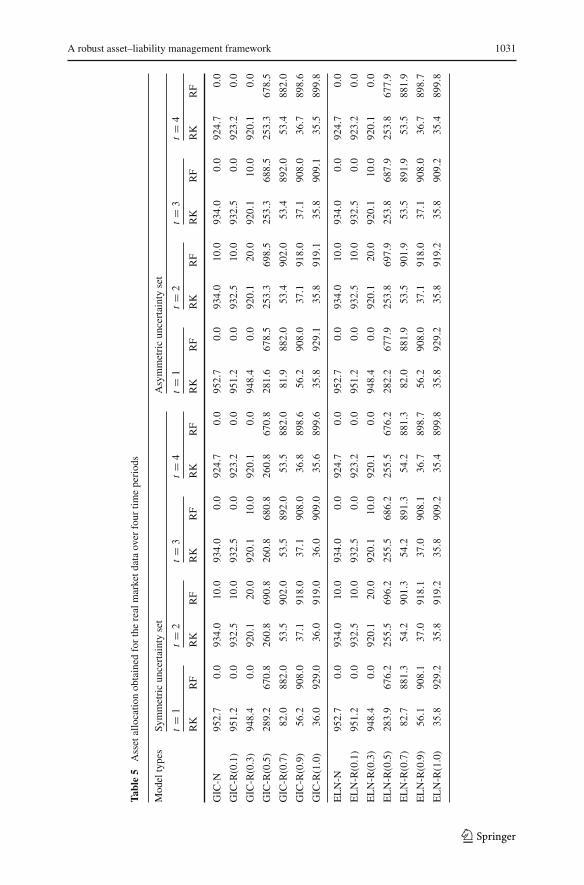
Table 5 presents the optimal asset allocations (in a risky asset and a risk-free assetabbreviated as RK and RF, respectively) obtained by solving the nominal and robustmodels under the normal market regime for the real market data for various values ofthe budget of robustness. We look at the first step of the rolling horizon simulationapproach (the step that is actually implemented). Note that the initial allocation of thecapital between risk-free and risky assets does not remain the same at the followingstages of the investment process due to updates for the future realizations of returns.The scenario-based stochastic programming ALM models for both types of productssuggests investing the whole capital (952.7) in the risky asset in the first time period.The asset allocation at the next stagesmay be different because it depends on the futurereturn realizations.
Based on the results in Table 5, it appears that the optimal asset allocation strategyobtained with the nominal model prefers to invest heavily in the risky asset rather thanthe risk-free asset at each time period. With regard to the robust strategy, the choice ofuncertainty sets and the structure of the guaranteed investment contract do not have anysubstantial impact on diversification (i.e., the relative magnitude of investments in therisky versus the risk-free asset). The level of diversification of the robust investmentstrategy depends on the pre-specified price of robustness. If the price of robustnessis low, the capital is invested mainly in the risky asset. As the price of robustnessincreases, the robust strategies become more risk-averse. Investment in the risky assetdecreases while investment in the risk-free asset increases to hedge for the increase inrisk associated with investing in the index. There appears to be a threshold (0.5) for
123
A robust asset–liability management framework 1031
Tabl
e5
Assetallocatio
nobtained
fortherealmarketd
ataover
four
timeperiods
Modeltypes
Symmetricuncertaintyset
Asymmetricuncertaintyset
t=
1t=
2t=
3t=
4t=
1t=
2t=
3t=
4
RK
RF
RK
RF
RK
RF
RK
RF
RK
RF
RK
RF
RK
RF
RK
RF
GIC
-N95
2.7
0.0
934.0
10.0
934.0
0.0
924.7
0.0
952.7
0.0
934.0
10.0
934.0
0.0
924.7
0.0
GIC
-R(0.1)
951.2
0.0
932.5
10.0
932.5
0.0
923.2
0.0
951.2
0.0
932.5
10.0
932.5
0.0
923.2
0.0
GIC
-R(0.3)
948.4
0.0
920.1
20.0
920.1
10.0
920.1
0.0
948.4
0.0
920.1
20.0
920.1
10.0
920.1
0.0
GIC
-R(0.5)
289.2
670.8
260.8
690.8
260.8
680.8
260.8
670.8
281.6
678.5
253.3
698.5
253.3
688.5
253.3
678.5
GIC
-R(0.7)
82.0
882.0
53.5
902.0
53.5
892.0
53.5
882.0
81.9
882.0
53.4
902.0
53.4
892.0
53.4
882.0
GIC
-R(0.9)
56.2
908.0
37.1
918.0
37.1
908.0
36.8
898.6
56.2
908.0
37.1
918.0
37.1
908.0
36.7
898.6
GIC
-R(1.0)
36.0
929.0
36.0
919.0
36.0
909.0
35.6
899.6
35.8
929.1
35.8
919.1
35.8
909.1
35.5
899.8
ELN-N
952.7
0.0
934.0
10.0
934.0
0.0
924.7
0.0
952.7
0.0
934.0
10.0
934.0
0.0
924.7
0.0
ELN-R
(0.1)
951.2
0.0
932.5
10.0
932.5
0.0
923.2
0.0
951.2
0.0
932.5
10.0
932.5
0.0
923.2
0.0
ELN-R
(0.3)
948.4
0.0
920.1
20.0
920.1
10.0
920.1
0.0
948.4
0.0
920.1
20.0
920.1
10.0
920.1
0.0
ELN-R
(0.5)
283.9
676.2
255.5
696.2
255.5
686.2
255.5
676.2
282.2
677.9
253.8
697.9
253.8
687.9
253.8
677.9
ELN-R
(0.7)
82.7
881.3
54.2
901.3
54.2
891.3
54.2
881.3
82.0
881.9
53.5
901.9
53.5
891.9
53.5
881.9
ELN-R
(0.9)
56.1
908.1
37.0
918.1
37.0
908.1
36.7
898.7
56.2
908.0
37.1
918.0
37.1
908.0
36.7
898.7
ELN-R
(1.0)
35.8
929.2
35.8
919.2
35.8
909.2
35.4
899.8
35.8
929.2
35.8
919.2
35.8
909.2
35.4
899.8
123

1032 N. Gulpinar et al.
the budget of robustness. As the budget of robustness gets higher than the threshold,the weight of the risky (risk-free) asset rapidly decreases (increases).
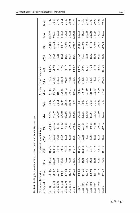
Simulation results: We are now concerned with performance comparison of the nom-inal, robust and stochastic approaches under normal and unfavorable market regimes.Table 6 presents the results of the rolling horizon simulation approach using generateddata with 10 risky assets and one risk-free asset within the normal (top) and unfavor-able with k = 1.0 (bottom) market regimes. In addition to the simulation statistics, wealso display the average realized transaction cost (T-cost) in Table 6. From the resultsin Table 6 we observe that
• The investment strategies obtained from the stochastic and nominal ALM modelsprovide higher expected wealth (as well as higher average transaction costs) thanthe investment strategies obtained from the robust ALM models using symmetricand asymmetric uncertainty sets under the normal market regime. This is not sur-prising because stochastic programmingmaximizes the expected profit over knowndiscrete scenarios whereas robust optimization uses a worst-case decision-makingcriterion. Moreover, under normal market regime, the future return scenarios arerealized as expected.
• If the future asset returns follow the same distribution as the distribution used asinput to the robust formulation, then the expected terminal wealth and the varianceof terminal wealth obtained by all robust models decrease when the robustnessbudget increases (see, for example, the results under normal market regime). Inother words, there is a trade-off between the average performance and the amountof protection desired. The nominal and stochastic investment strategies providehigher average wealth than the robust strategy for a high budget of robustness.
• On the other hand, the robust investment strategies at (high) budget of robustnessappear to perform better than those obtained with the stochastic and nominalformulations in unfavorable market regimes. Recall that in the unfavorable marketregime, the future return realizations are generated by the expected value μ − kσ
(that is k standard deviation lower than the estimated expected value from thedata) and the standard deviation (σ ). As shown in Table 6, the terminal wealthobtained by all robust models when future realized asset returns are worse thanexpected increases as the robustness budget increases, and the variance of finalwealth decreases. Both the nominal and the stochastic investment strategies resultin lower expected wealth than the robust strategy for symmetric and asymmetricuncertainty sets at high value of the price of robustness. This argues for usingrobust optimization in unfavorable market scenarios.
• The robust strategies with asymmetric uncertainty sets result in slightly higherwealth (and/or lower variance) than the wealth obtained for robust strategies gen-eratedwith the symmetric uncertainty sets formulation for any degree of robustness(apart from the lowest value 0.1) under unfavorablemarket regimes. This is becausethe future return realizations for the generated data have asymmetric characteris-tics. It appears that the distribution of various price realizations and the choice ofuncertainty set impact the performance of the robust investment strategy.
• In both market regimes, the robust GIC models result in a slightly higher expectedvalue and variance of wealth than the robust ELN models regardless of the type
123
A robust asset–liability management framework 1033
Tabl
e6
Rollin
ghorizonsimulationstatisticsobtained
forthe10-assetcase
Normalmarketregim
eSy
mmetricuncertaintyset
Asymmetricuncertaintyset
ALM
models
Mean
Sdev
VaR
CVaR
Min
Max
T-cost
Mean
Sdev
VaR
CVaR
Min
Max
T-cost
GIC
-N28
7.05
345.82
−166
.95
−166
.95
−258
.80
1265
.55
41.87
287.05
345.82
−166
.95
−166
.95
−258
.80
1265
.55
41.87
GIC
-R(0.1)
264.87
259.55
−102
.70
−102
.70
−235
.59
943.39
38.79
263.92
257.59
−98.98
−98.98
−235
.24
932.01
38.33
GIC
-R(0.3)
221.99
168.88
−14.18
−14.18
−85.46
624.39
32.61
218.41
161.89
−8.15
−8.15
−71.31
607.08
31.75
GIC
-R(0.5)
198.51
126.40
30.75
30.75
−61.39
525.80
29.25
195.55
121.86
41.96
41.96
−62.17
511.78
28.61
GIC
-R(0.7)
174.82
99.22
43.35
43.35
−48.63
432.86
25.36
168.72
92.64
48.77
48.77
−45.05
408.96
24.87
GIC
-R(0.9)
152.88
78.56
42.18
42.18
−29.10
352 .88
22.71
149.34
75.10
45.74
45.74
−29.14
339.15
22.01
GIC
-S28
9.23
331.83
−146
.87
−146
.87
−240
.87
1235
.66
41.78
289.23
331.83
−146
.87
−146
.87
−240
.87
1235
.66
41.78
ELN-N
148.83
199.52
−166
.95
−166
.95
−258
.80
657.78
41.80
148.83
199.52
−166
.95
−166
.95
−258
.80
657.78
41.80
ELN-R
(0.1)
147.20
145.65
−102
.66
−102
.66
−235
.63
491.18
41.09
146.79
144.47
−99.01
−99.01
−235
.06
485.39
41.50
ELN-R
(0.3)
122.80
68.42
5.39
5.39
−72.53
261.42
34.73
121.59
65.64
12.35
12.35
−74.82
257.66
33.84
ELN-R
(0.5)
116.92
55.76
33.59
33.59
−60.63
230.54
32.63
115.99
54.31
41.32
41.32
−61.42
227.56
33.00
ELN-R
(0.7)
108.12
46.38
43.35
43.35
−48.65
193.42
30.89
105.85
44.00
48.76
48.76
−45.05
184.54
29.99
ELN-R
(0.9)
99.77
39.10
42.26
42.26
−29.12
172.60
28.28
98.30
37.90
45.80
45.80
−29.20
170.00
28.26
ELN-S
144.35
190.79
−161
.30
−161
.30
−269
.32
627.93
40.69
144.35
190.79
−161
.30
−161
.30
−269
.32
627.93
40.69
123

1034 N. Gulpinar et al.
Tabl
e6
continued
Unfavorablemarketregim
eSy
mmetricuncertaintyset
Asymmetricuncertaintyset
ALM
models
Mean
Sdev
VaR
CVaR
Min
Max
T-cost
Mean
Sdev
VaR
CVaR
Min
Max
T-cost
GIC
-N−2
53.13
206.11
−524
.47
−524
.47
−583
.74
327.78
43.58
−253
.13
206.11
−524
.47
−524
.47
−583
.74
327.78
43.58
GIC
-R(0.1)
−257
.41
155.94
−479
.71
−479
.71
−556
.02
147.31
39.94
−257
.53
154.80
−477
.06
−477
.06
−555
.51
141.02
38.95
GIC
-R(0.3)
−254
.90
102.88
−400
.04
−400
.04
−442
.71
−10.71
34.33
−254
.84
98.84
−394
.13
−394
.13
−434
.53
−18.20
32.41
GIC
-R(0.5)
−253
.14
77.89
−353
.38
−353
.38
−416
.06
−51.29
30.71
−252
.99
75.27
−347
.40
−347
.40
−414
.82
−57.44
28.81
GIC
-R(0.7)
−241
.37
62.03
−322
.99
−322
. 99
−383
.29
−80.42
26.29
−230
.14
57.88
−304
.58
−304
.58
−365
.67
−80.46
26.34
GIC
-R(0.9)
−215
.53
49.40
−285
.26
−285
.26
−331
.43
−90.76
23.14
−214
.92
47.37
−280
.26
−280
.26
−328
.92
−96.25
22.10
GIC
-S−2
52.25
197.04
−515
.81
−515
.81
−582
.69
329.92
42.01
−252
.25
197.04
−515
.81
−515
.81
−582
.69
329.92
42.01
ELN-N
−259
.09
191.76
−524
.47
−524
.47
−583
.74
188.89
42.37
−259
.09
191.76
−524
.47
−524
.47
−583
.74
188.89
42.37
ELN-R
(0.1)
−258
.30
153.41
−479
.65
−479
.65
−556
.04
98.32
42.36
−258
.39
152.30
−477
.01
−477
.01
−555
.39
95.11
42.25
ELN-R
(0.3)
−254
.53
93.84
−382
.82
−382
.82
−432
.85
−23.02
35.27
−254
.43
90.36
−376
.33
−376
.33
−432
.46
−30.17
34.88
ELN-R
(0.5)
−253
.09
77.17
−351
.51
−351
.51
−415
.01
−52.89
33.16
−252
.96
74.63
−347
.41
−347
.41
−413
.78
−59.02
33.64
ELN-R
(0.7)
−241
.37
62.03
−322
.99
−322
. 99
−383
.30
−80.46
32.76
−230
.16
57.89
−304
.61
−304
.61
−365
.70
−80.47
30.61
ELN-R
(0.9)
−215
.53
49.36
−285
.16
−285
.16
−331
.40
−90.86
29.56
−214
.92
47.37
−280
.20
−280
.20
−328
.95
−96.21
29.40
ELN-S
−258
.68
187.35
−517
.76
−517
.76
−569
.56
175.43
42.22
−258
.68
187.35
−517
.76
−517
.76
−569
.56
175.43
42.22
123

A robust asset–liability management framework 1035
Fig. 1 Distribution of final wealth for the ALM models using ELN (top) and GIC (bottom) productsin the normal (left) and unfavorable (right) market regimes. Clockwise from top left: an ELN stochasticformulation under a normal market regime; an ELN stochastic formulation under a unfavorable marketregime; a GIC stochastic formulation under a unfavorable market regime; a GIC stochastic formulationunder a normal market regime
of uncertainty sets. This is because the extra return on the terminal wealth is paidto the holder of ELNs. On the other hand, we observe that the ALM models forGIC products produce lower expected transaction cost than those provided by theALM models using ELN regardless the market conditions.
Figure 1 displays the distribution of the final wealth computed from the simulationexperiments using data for 10 assets with 4 time periods. In the unfavorable marketregime, the future return realizations are generated with a lower mean (μ − σ). Thehistograms of final wealth outcomes for the robust optimization models with price ofrobustness of 0.5 and 1.0 are plotted with solid lines.
Interestingly, the relative advantage of the robust strategies increases as the mar-ket worsens - the position of the distribution of wealth under the robust strategiesrelative to the other two types of strategies is farther to the right. Hence, the robustapproaches represent effective hedging strategies with respect to the given risk expo-sures (uncertainties). This can be viewed as a strong argument for adopting them inpractice.
Sensitivity analysis: We also run a sensitivity analysis to determine the possible effectof the selection of model parameters on the performance of the investment strategies.We consider differentmarket conditionswhere future realizations of uncertain parame-
123

1036 N. Gulpinar et al.
Fig. 2 Average wealth obtained for the ALM strategies for ELN (left) and GIC (right) products using 2,10, 20 and 30 (top to bottom panels) assets in various market regimes
ters are generated with different expected value (μ−kσ) and the same variance (σ ) asestimated from the data. As k varies from 0 (normal market regime) to 1, the expectedvalues of the returns in future scenarios decrease. Next, we summarize observationsabout the effect of various parameters and factors on the ALM investment strategiesobtained with the nominal, stochastic and robust optimization models.
• Number of risky assets and diversification: We first extend the simulation exper-iments conducted for the 2-asset real market case to a set of generated data witha larger number of assets (10, 20 and 30). The average wealth obtained with thestochastic, nominal and robust (at fixed budget of robustness of 0.3, 0.7 and 1.0)strategies is displayed in Fig. 2. As the market conditions deteriorate, the robuststrategies with high budget of robustness outperform both the nominal and the
123

A robust asset–liability management framework 1037
Fig. 3 Performance comparison of the ALM strategies for ELN (top) and GIC (bottom) products in variousmarket regimes obtained by different simulation methods using 10 (left) and 30 (right) assets
stochastic ones. However, the gap between the expected wealth obtained with thestochastic programming and the robust optimization models diminishes as thenumber of assets increases due to the impact of diversification. Diversificationappears to help the stochastic programming strategies do well even in unfavorablemarket conditions. For instance, while the deteriorating point for stochastic pro-gramming strategies is at k ≈ 0.15 for the 2-asset case, it is at k ≈ 0.5 for the10-asset case.
• Performance evaluation approaches:Weconsider static and dynamic performanceevaluation approaches using cases with 10 and 30 assets. As explained before, therolling horizon method updates the strategy as more info is received whereas thefixed horizon applies the prior strategy over time. Their results are shown in Fig. 3.We see that the average wealth obtained by the robust models is higher than theone obtained by the nominal model for smaller values of k (at lower levels of theunfavorable regime) if the number of assets is large. This is because diversificationhas a stronger effect when there are more investment alternatives.
• Uncertainty sets: In order to understand how the size and the shape of the sym-metric and asymmetric uncertainty sets affect the robust investment strategies, wevary the budget of robustness for the uncertainty sets associated with the uncertaincoefficients in the objective function and the balance constraints. The numericalexperiments indicate that the budget of robustness for the funding ratio constraintsdoes not have a substantial effect on the investment decisions; hence those resultson are not included here.
123
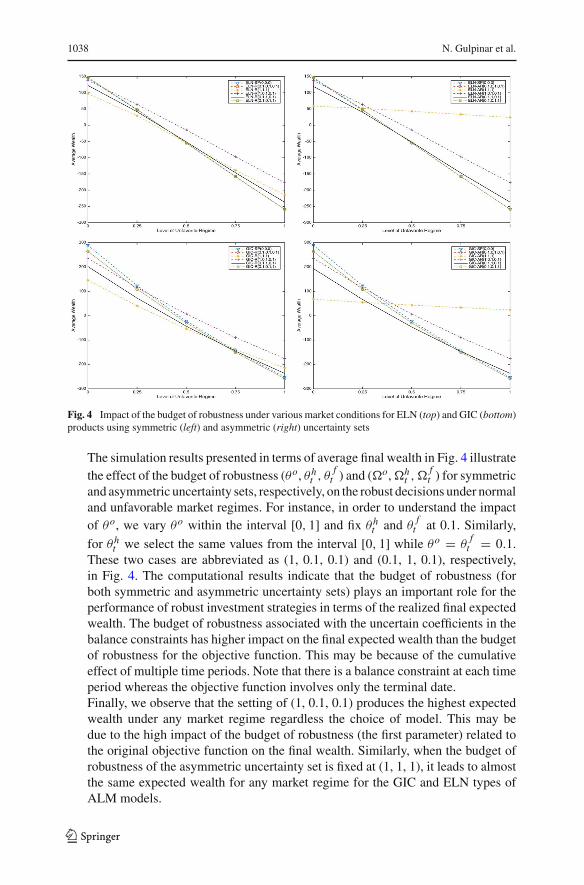
1038 N. Gulpinar et al.
Fig. 4 Impact of the budget of robustness under various market conditions for ELN (top) and GIC (bottom)products using symmetric (left) and asymmetric (right) uncertainty sets
The simulation results presented in terms of average final wealth in Fig. 4 illustratethe effect of the budget of robustness (θo, θh
t , θf
t ) and (�o,�ht ,�
ft ) for symmetric
and asymmetric uncertainty sets, respectively, on the robust decisions under normaland unfavorable market regimes. For instance, in order to understand the impactof θo, we vary θo within the interval [0, 1] and fix θh
t and θf
t at 0.1. Similarly,
for θht we select the same values from the interval [0, 1] while θo = θ
ft = 0.1.
These two cases are abbreviated as (1, 0.1, 0.1) and (0.1, 1, 0.1), respectively,in Fig. 4. The computational results indicate that the budget of robustness (forboth symmetric and asymmetric uncertainty sets) plays an important role for theperformance of robust investment strategies in terms of the realized final expectedwealth. The budget of robustness associated with the uncertain coefficients in thebalance constraints has higher impact on the final expected wealth than the budgetof robustness for the objective function. This may be because of the cumulativeeffect of multiple time periods. Note that there is a balance constraint at each timeperiod whereas the objective function involves only the terminal date.Finally, we observe that the setting of (1, 0.1, 0.1) produces the highest expectedwealth under any market regime regardless the choice of model. This may bedue to the high impact of the budget of robustness (the first parameter) related tothe original objective function on the final wealth. Similarly, when the budget ofrobustness of the asymmetric uncertainty set is fixed at (1, 1, 1), it leads to almostthe same expected wealth for any market regime for the GIC and ELN types ofALM models.
123

A robust asset–liability management framework 1039
7 Concluding remarks
In this paper, we considered the asset–liability management problem for investmentproducts with guarantees where the optimal structure of the underlying fund is deter-mined and exogenous uncertainties in asset returns and interest rates are incorporatedin the model using a multi-period robust optimization framework. We introduceda tractable robust approach to solving the problem using symmetric and asymmet-ric uncertainty sets, and described practical approaches for estimating the inputs.The performance of the robust formulations of ALM models for investment productswith guarantees were evaluated in computational experiments with simulated and realmarket data, contrasted with the performance of strategies based on stochastic pro-gramming, and benchmarked against the performance of expected value optimization.The robust investment strategies have better performance in terms of variability andrelative return under unfavorable market regimes where the future realizations followprobability distributions with lower means than expected. The numerical results alsoshow that the robust model parameters and the size of the uncertainty sets play animportant role for the performance of robust optimization models.
When deciding on the approach for determining the optimal structure of portfoliosunderlying investment products with guarantees, one should note that there are philo-sophical differences between the application of the robust optimization approach andthe stochastic programming approach. First, the representation of the uncertainties isdone differently. In the stochastic programming approach, one solves the optimiza-tion problem to come up with an exact strategy to be followed for each scenario.One expects that if nature behaves very similarly to the scenarios one has generated,the optimal strategy will perform well on average. The robust optimization approachattempts to find a more general strategy (one not tied to specific scenarios) that workswell in terms of worst-case performance. This is effective in practice, as demonstratedin the computational experiments. Second, the sizes of the resulting optimization prob-lems are very different. Generally, robust optimization formulations based on summarymeasures of the probability distributions of the uncertainties have a much smaller sizethan stochastic programming formulations. This allows for the calculations to be runmultiple times with little additional computational effort for a range of design parame-ters for investment products with guarantees, and addresses the problem of the optimalpricing of such contracts as well.
Open Access This article is distributed under the terms of the Creative Commons Attribution 4.0 Interna-tional License (http://creativecommons.org/licenses/by/4.0/), which permits unrestricted use, distribution,and reproduction in any medium, provided you give appropriate credit to the original author(s) and thesource, provide a link to the Creative Commons license, and indicate if changes were made.
References
Bacinello AR (2003) Fair valuation of a guaranteed life insurance participating contract embedding asurrender option. J Risk Insur 70:461–487
Ben-Tal A, Nemirovski A (1998) Robust convex optimization. Math Oper Res 23(4):769–805
123

1040 N. Gulpinar et al.
Ben-Tal A, Margalit T, Nemirovski A (2000) Robust modeling of multi-stage portfolio problems. In: FrenkH, Roos K, Terlaky T, Zhang S (eds) High-performance optimization. Kluwer Academic Publishers,Dordrecht, pp 303–328
Ben-Tal A, El Ghaoui L, Nemirovski A (2009) Robust optimization. Princeton University Press, PrincetonBertsimas D, Pachamanova D (2008) Robust multiperiod portfolio management in the presence of transac-
tion costs. Comput Oper Res 35:3–17Bertsimas D, Pachamanova D, Sim M (2004) Robust linear optimization under general norms. Oper Res
Lett 32:510–516Boender G, Dert C, Heemskerk F, Hoek H (2005) A scenario approach of ALM. In: Zenios SA, Ziemba
WT (eds) Handbook of asset and liability management. North-Holland, AmsterdamBrennan MJ, Schwartz ES (1976) The pricing of equity-linked life insurance policies with an asset value
guarantee. J Financ Econ 3(3):195–213Brennan MJ, Schwartz ES (1979) Alternative investment strategies for the issuers of equity linked life
insurance policies with an asset value guarantee. J Bus 52(1):63–93Chen X, Sim M, Sun P (2007) A robust optimization perspective on stochastic programming. Oper Res
55(6):1058–1071Consigli G, Dempster MAH (1998) Dynamic stochastic programming for asset-liability management. Ann
Oper Res 81:131–162Consiglio A, Cocco F, Zenios SA (2001) The value of integrative risk management for insurance products
with guarantees. J Risk Financ 2(3):6–16Consiglio A, Saunders D, Zenios SA (2006) Asset and liability management for insurance products with
minimum guarantees: the UK case. J Bank Financ 30:645–667Consiglio A, Cocco F, Zenios SA (2008) Asset and liability modeling for participating policies with guar-
antees. Eur J Oper Res 186(1):380–404Dantzig GB, Infanger G (1993)Multi-stage stochastic linear programs for portfolio optimization. Ann Oper
Res 45:59–76Duffee G (2002) The long-run behavior of firms stock returns: evidence and interpretations. Working paper,
Haas School of Business, University of California at Berkeley, Berkeley, CAEl Ghaoui L, Lebret H (1997) Robust solutions to least-squares problems with uncertain data. SIAM J
Matrix Anal Appl 18(4):1035–1064Escudero LF, Garín A, Merino M, Pérez G (2009) On multistage stochastic integer programming for
incorporating logical constraints in asset and liability management under uncertainty. Comput ManagSci 6:307–327
Fabozzi F, Kolm P, Pachamanova D, Focardi S (2007) Robust portfolio optimization and management.Wiley, Hoboken
Ferstl R,Weissensteiner A (2011) Asset-liability management under time varying investment opportunities.J Bank Financ 35(1):182–192
Gerstner T, Griebel M, Holtz M, Goschnick R, Haep M (2008) A general asset-liability management modelfor the efficient simulation of portfolios of life insurance policies. Insur Math Econ 42:704–716
Goldfarb D, Iyengar G (2003) Robust portfolio selection problem. Math Oper Res 28(1):1–37Gondzio J, Kouwenberg R (2001) High performance computing for asset-liability management. Oper Res
49(6):879–891Goyal A,Welch I (2008) A comprehensive look at the empirical performance of equity premium prediction.
Rev Financ Stud 21:1455–1508Gulpinar N, Pachamanova D (2013) A robust optimization approach to asset-liability management under
time-varying investment opportunities. J Bank Financ 37(6):2031–2041Gulpinar N, Rustem B (2007) Worst-case optimal robust decisions for multi-period portfolio optimization.
Eur J Oper Res 183(3):981–1000Gulpinar N, RustemB, Settergren R (2004) Simulation and optimization approaches to scenario generation.
J Econ Dyn Control 28:1291–1315Hardy M (2003) Investment guarantees: modeling and risk management for equity-linked life insurance.
Wiley, New YorkKlaassen P (1998) Financial asset-pricing theory and stochastic programming models for asset-liability
management. Manag Sci 44(1):31–48Kouwenberg R (2001) Scenario generation and stochastic programming models for asset liability manage-
ment. Eur J Oper Res 134(2):279–292
123

A robust asset–liability management framework 1041
Löfberg J (2004) YALMIP: a toolbox for modeling and optimization in MATLAB. In: Proceedings of theCACSD conference, Taipei, Taiwan
Mallier R, Alobaidi G (2002) Pricing equity-linked debt using the Vasicek model. Acta Math Univ Comen71(2):211–220
Miltersen KR, Persson SA (2003) Guaranteed investment contracts: distributed and undistributed excessreturn. Scand Actuar J 4:257–279
Natarajan K, Pachamanova D, SimM (2008) Incorporating asymmetric distributional information in robustvalue-at-risk optimization. Manag Sci 54(3):573–585
Natarajan K, Pachamanova D, Sim M (2009) Constructing risk measures from uncertainty sets. Oper Res57(5):1129–1141
Nietert B (2003) Portfolio insurance and model uncertainty. OR Spectr 25:295–316Oguzsoy CB, Guven S (2007) Robust portfolio planning in the presence of market anomalies. OMEGA:
Int J Manag Sci 35(1):1–6Pachamanova DA, Fabozzi FJ (2016) Portfolio construction and analytics. Wiley, HobokenPae Y, Sabbaghi N (2014) Log-robust portfolio management after transaction costs. OR Spectr 36:95–112Pinar M (2007) Robust scenario optimization based on downside-risk measure for multi-period portfolio
selection. OR Spectr 29(2):295–309Powell WB (2011) Approximate dynamic programming. Wiley, New YorkRamaswami M, Lieberman PK, Baez G (2001) Equity-linked notes. Global Equity Derivatives, Lehman
BrothersSoyster AL, Murphy FH (2013) A unifying framework for duality and modeling in robust linear programs.
OMEGA: Int J Manag Sci 41(6):984–997Stiefel JD (1984) The guaranteed investment contract (GIC). Soc Actuar 36:265–285Toy WW, Ryan MD (2000) Public equity-linked debt. In: Francis JC, Toy WW, Whittaker JG (eds) The
handbook of equity derivatives. Wiley, New York, pp 329–342Valle CA, Meade N, Beasley JE (2014) Absolute return portfolios. OMEGA: Int J Manag Sci 45:20–41Walsh MW (2008) Where did AIG’s cash go? The New York Times, October 30Ziemba WT, Mulvey JM (1998) Worldwide asset and liability modeling. Cambridge University Press,
Cambridge
123