a role of humic matter and ore oxidation in - circle
TRANSCRIPT

A ROLE OF HUMIC MATTER AND ORE OXIDATION IN RHEOLOGY
OF OIL SAND SLURRIES AND IN BITUMEN EXTRACTION
by
LEOPOLDO GUTIERREZ
B.Sc., University of Concepcion, 2001
A THESIS SUBMITTED IN PARTIAL FULFILLMENT OF
THE REQUIREMENTS FOR THE DEGREE OF
DOCTOR OF PHILOSOPHY
in
THE FACULTY OF GRADUATE STUDIES
(Mining Engineering)
THE UNIVERSITY OF BRITISH COLUMBIA
(Vancouver)
April 2013
© Leopoldo Gutierrez, 2013
ii
ABSTRACT
Eight oil sands ores were tested in order to quantify the levels of humic acids in these
samples through the alkali extraction test originally developed to determine the oxidation of
bituminous metallurgical coals. The test gives a concentration of humic acids released from ores,
which in combination with the measurement of the total organic carbon content in the alkali
extracts provides a measure of ore/bitumen weathering. It was found that poor ores exhibited the
highest tendency to leach large amounts of humic acids per gram of bitumen in the samples which
was quantified using the absorbance at 520 nm obtained from the UV/visible spectra.
The results of contact angle measurements of water on bitumen showed that bitumen
became more hydrophilic as pH increased, and that the hydrophobicity of bitumen drastically
decreased when the sample was artificially oxidized. Additionally, the results suggested that humic
acids make bitumen hydrophilic only if they are part of the internal/surface bitumen structure.
Slurries of good ores displayed higher yield stresses than slurries of poor ores. This result is
explained by the higher bitumen concentration existing in slurries of good ores which leads to more
aggregation. Additionally, it was shown that bitumen oxidation/hydrophobicity also affected the
rheology of oil sands slurries which also explains that slurries of poor ores displayed lower
cohesion/aggregation than slurries of good ores. Yield stress data agreed with data obtained from
power draw measurements that showed that good processing ores required more power for mixing.
Extraction data obtained from flotation experiments indicated that the role of humic acids naturally
present in the ores was basically that of a depressant of bitumen since poor ores contained the
highest proportion of humic acids per gram of bitumen.
Overall, it is possible to assess the processability of oil sand ores by quantifying the
occurrence of humic acids in the ores, and to correlate ore processability with the rheology of oil
sands slurries. Although poor ores are characterized by lower viscosities and lower power
requirements during mixing, the presence of humic acids in these ores and their depressing action
also contribute to lower bitumen recoveries.

iii
PREFACE
The definition and design of the research program, the analysis of the experimental data and
the preparation of the thesis manuscript were carried out by the author in consultation with the
research supervisor Dr. Marek Pawlik. Apart from the Dean-Stark analyses of the oil sands samples
that were done by a commercial Lab, all the experimental work involved was carried out 100% by
the author of this thesis.

iv
TABLE OF CONTENTS
ABSTRACT ........................................................................................................................................... ii
PREFACE ............................................................................................................................................. iii
TABLE OF CONTENTS .................................................................................................................... iv
LIST OF TABLES .............................................................................................................................. vii
LIST OF FIGURES ........................................................................................................................... viii
ACKNOWLEDGEMENTS ............................................................................................................. xiii
1 Introduction .................................................................................................................................. 1
1.1 Importance of this study .......................................................................................................... 1
1.2 Research objectives .................................................................................................................. 3
2 Literature review .......................................................................................................................... 5
2.1 Composition of oil sand ores ................................................................................................... 5
2.1.1 General properties ..................................................................................................................... 5
2.1.2 Sand fraction .............................................................................................................................. 6
2.1.3 Bitumen ...................................................................................................................................... 6
2.2 Processing of oil sand ores ....................................................................................................... 8
2.2.1 Process description .................................................................................................................... 8
2.2.2 Bitumen liberation and aeration .............................................................................................. 10
2.2.3 Research methods used in oil sands processing ..................................................................... 11
2.3 Effect of different variables on oil sands processing .......................................................... 13
2.3.1 Effect of ore properties ............................................................................................................ 14
2.3.2 Effect of water chemistry ........................................................................................................ 15
2.3.3 Effect of operating conditions ................................................................................................. 18
2.4 Oxidation of oil sands............................................................................................................. 20
2.5 Interactions of humic acids and their effect on rheology of suspensions ........................ 22
2.6 Hydrophobic interactions ...................................................................................................... 25
2.7 Rheology .................................................................................................................................. 27
2.7.1 General definitions .................................................................................................................. 27
2.7.2 Typical rheological responses ................................................................................................. 29
2.7.3 Flow curve modeling ............................................................................................................... 32
2.7.4 Rheometry ................................................................................................................................ 37
2.7.4.1 Concentric cylinder rheometers ....................................................................................... 38

v
2.7.4.2 Errors of measurements in concentric cylinder rheometers ............................................ 41
2.7.4.3 Infinite gap approach........................................................................................................ 43
2.7.5 Micro-rheology of suspensions ............................................................................................... 44
2.7.6 Effect of particle size and particle size distribution on rheology of suspensions .................. 45
2.7.7 Yield stress determination ....................................................................................................... 47
2.7.7.1 General considerations ..................................................................................................... 47
2.7.7.2 Methods for determining yield stress .............................................................................. 48
2.7.8 Surface chemistry and rheology of quartz suspensions .......................................................... 55
3 Experimental program .............................................................................................................. 58
3.1 Samples and reagents ............................................................................................................. 61
3.1.1 Oil sands ores ........................................................................................................................... 61
3.1.2 Quartz and kaolinite samples .................................................................................................. 65
3.1.3 Reagents ................................................................................................................................... 65
3.2 Procedures, methods and equipment ................................................................................... 66
3.2.1 Alkali-extraction tests .............................................................................................................. 66
3.2.2 Extraction tests at milder conditions ....................................................................................... 68
3.2.3 Contact angle measurements ................................................................................................... 69
3.2.4 Fourier transform infrared spectroscopy (FTIR) .................................................................... 70
3.2.5 Effect of humic acids on rheology .......................................................................................... 71
3.2.6 Effect of humic acids on bitumen extraction .......................................................................... 73
3.2.7 Yield stress measurements ...................................................................................................... 73
3.2.8 Power draw measurements ...................................................................................................... 77
3.2.9 Evaluation of the extractability of bitumen from different ores ............................................ 78
4 Results and discussion ................................................................................................................ 80
4.1 Study of the occurrence of humic acids in oil sands ores .................................................. 80
4.1.1 Applicability of the alkali extraction tests to oil sand ores .................................................... 80
4.1.2 Extractions of humic acids at pH values of 8.5 and 10 .......................................................... 88
4.1.3 Association of humic acids with ore components .................................................................. 89
4.1.4 Bitumen contact angles and their connection to oxidation of oil sands ................................. 96
4.1.5 Effect of humic acids on rheology of oil sand suspensions ................................................. 104
4.1.6 Effect of humic acids on bitumen extraction ........................................................................ 107
4.2 Rheological characterization .............................................................................................. 110
4.2.1 Theoretical framework on rheology of oil sands slurries ..................................................... 110

vi
4.2.2 Effect of bitumen on the yield stress of concentrated slurries (64-73 wt.% solids) ............ 112
4.2.2.1 Vane tests........................................................................................................................ 113
4.2.2.2 Slump tests ..................................................................................................................... 125
4.2.2.3 Relaxation method ......................................................................................................... 127
4.2.2.4 Flow curve extrapolation (equilibrium flow curves from stress decay tests) ............... 128
4.2.2.5 Comparison of the yield stress values obtained using the vane, slump, relaxation, and flow curve extrapolation methods .............................................................................................. 132
4.2.3 Effect of ore oxidation on the cohesiveness of oil sands slurries ........................................ 138
4.2.4 Effect of ore quality on the yield stress ................................................................................ 140
4.2.5 Power draw measurements on oil sands slurries (45 wt.% solids) ...................................... 141
4.3 Evaluation of the extractability of bitumen from different ores .................................... 147
4.3.1 Modeling of flotation experiments of bitumen ..................................................................... 147
4.3.2 Flotation experiments with actual oil sands ores .................................................................. 150
4.3.2.1 Reproducibility of flotation experiments ....................................................................... 150
4.3.2.2 Bitumen extraction ......................................................................................................... 152
4.3.3 A method for assessing processability/quality of oil sands ores based on the alkali extraction test .................................................................................................................................. 160
5 Conclusions ............................................................................................................................... 164
6 Recommendations for future work ........................................................................................ 169
Bibliography ...................................................................................................................................... 170
Appendices ......................................................................................................................................... 187
Appendix A: Calibration curves of Abs520 and TOC versus Aldrich humic acid concentration. .................................................................................................................................. 187
Appendix B: Procedure followed to determine the Tdl values from the torque versus time curves obtained from vane tests. ................................................................................................... 188
Appendix C: Torque versus vane rotation curves obtained from vane tests on slurries of ores 3, 5, and 6 tested at 70 wt.% solids. .............................................................................................. 190
Appendix D: Method used to calculate the standard deviation of yield stresses calculated from vane data. ............................................................................................................................... 191

vii
LIST OF TABLES
Table 2.1. Variables that affect the efficiency of the process of bitumen extraction from oil sands
ores. ...................................................................................................................................... 14
Table 3.1. Structure of the experimental program followed in this thesis.=solids content. ............ 60
Table 3.2. Composition of the oil sands samples tested. ..................................................................... 61
Table 3.3. Characterization of the sand fraction of the oil sands samples tested. (*) Calculated based
on particle size distribution assuming spherical particles. ................................................. 63
Table 3.4. Mineralogy of the sand fraction of oil sands samples tested. These results were obtained
by XRD. ............................................................................................................................... 64
Table 4.1. Results obtained from alkali extraction tests on samples of toluene-separated sand (TSS)
and toluene-extracted bitumen (TEB). ................................................................................ 92
Table 4.2. Numerical data of the results presented in Figures 4.29 to 4.31. is the standard
deviation obtained from triplicates measurements. .......................................................... 135
Table 4.3. Numerical data of the results presented in Figures 4.32 and 4.33. is the standard
deviation obtained from triplicates measurements. .......................................................... 138
Table 4.4. Parameters of flotation model. .......................................................................................... 155

viii
LIST OF FIGURES
Figure 2.1. Structural model of Athabasca oil sands (Takamura, 1982. With permission). ................ 6
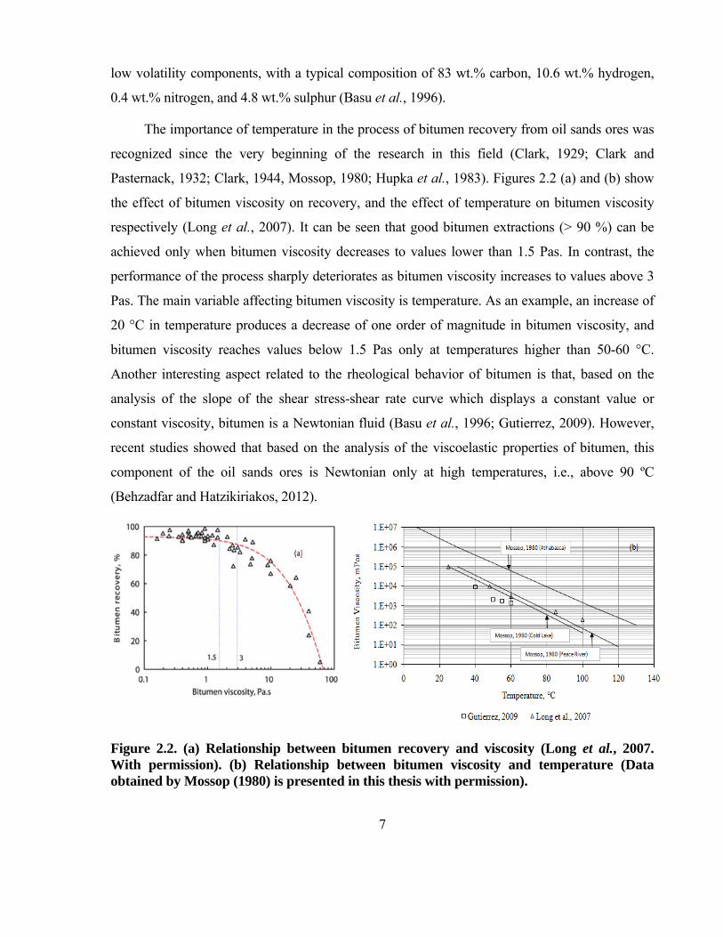
Figure 2.2. (a) Relationship between bitumen recovery and viscosity (Long et al., 2007. With
permission). (b) Relationship between bitumen viscosity and temperature (Data obtained
by Mossop (1980) is presented in this thesis with permission). .......................................... 7
Figure 2.3. Typical flow diagram of oil sands processing. .................................................................... 9
Figure 2.4. Typical ways of bitumen-air attachments at different temperatures. ............................... 11
Figure 2.5. Repulsive (positive values) and adhesive forces (insert) between bitumen-silica surfaces
as a function of separation distance and pH (Liu et al., 2003. With permission). ............. 17
Figure 2.6. Schematic of simple shear strain. v=velocity (m/s), y=vertical position (m), l=gap
between parallel plates (m), =shear stress (Pa). ................................................................ 28
Figure 2.7. Common relationships between shear stress and shear rate. ............................................ 32
Figure 2.8. (a) Cross-section, and (b) a fluid element in a concentric cylinder viscometer. .............. 39
Figure 2.9. Dynamic and static yield stresses (Cheng, 1986. With permission). ............................... 48
Figure 2.10. (a) Diagram of the vane and (b) the vane inserted into the sample. ............................... 50
Figure 2.11. Typical torque-time curve obtained from the vane test. ................................................. 51
Figure 2.12. Schematic of the slump test. (a) Cylinder filled with slurry, (b) slurry after slumping. 54
Figure 3.1. Particle size distributions of the sand fractions of the tested oil sands ores. .................... 62
Figure 3.2. Particle size distributions of pure samples of fine quartz, coarse quartz, and fine
kaolinite................................................................................................................................ 66
Figure 3.3. (a) Illustration of contact angle measurements. (b) Example of the determination of
contact angle by the software of the FTA 1000 Drop Shape Instrument. Air bubble
profiles and contact angles for (c) a very hydrophobic bitumen and for (d) a slightly
hydrophobic bitumen. .......................................................................................................... 70
Figure 3.4. Schematic of attenuated total reflection spectroscopy (ATR). ......................................... 71
Figure 3.5. Pictures of the vanes used in the experiments. .................................................................. 74

ix
Figure 3.6. Cylinder used in slump tests and a slumped slurry of ore 2 at 68 wt.% solids. ............... 75
Figure 3.7. Representation of the elongated fixture used in rheological measurements and the Haake
Rotovisco VT550. r1= 16.5 mm, r2= 19.0 mm, r3= 20.0 mm, r4= 23.03 mm. ................... 76
Figure 3.8. Schematic of the turn-table setup. ..................................................................................... 79
Figure 4.1. Images of the alkali extracts obtained from alkali extraction tests on ores 1 through 8. . 81
Figure 4.2. (a) UV-Visible spectra and (b) total organic carbon of extracts obtained from alkali-
extraction tests on the ore samples. ..................................................................................... 83
Figure 4.3. (a) Correlation between TOC and Absorbance at 520 nm (Abs520) of solutions obtained
from alkali-extraction tests on the 8 oil sands samples. (b) Correlation between
Absorbance at 520 nm (Abs520) and the ratio of the fines content (-44 m size fraction)
to bitumen content. .............................................................................................................. 84
Figure 4.4. (a) Equivalent content of Aldrich humic acids in the tested ores in wt.% and (b) in grams
per ton of bitumen................................................................................................................ 85
Figure 4.5. Comparison between the UV/Visible spectra of solutions obtained from alkali-extraction
tests and spectra of solutions of Aldrich Humic Acids. Solutions of Aldrich HA were
prepared at the same TOC values as those of the alkali-extracted solutions. .................... 87
Figure 4.6. Abs520 of solutions obtained after contacting a given amount of each ore containing 1 g
of bitumen with 0.01 M NaCl solutions at pH 8.5 and 10.0, and at 50 °C. ....................... 88
Figure 4.7. Surface tension and its correlation with the TOC values of solutions obtained at 50 °C
and pH values of 8.5 and 10. ............................................................................................... 90
Figure 4.8. FTIR spectra of the oil sands samples. Band assignments were made according to
Socrates (1980). ................................................................................................................... 94
Figure 4.9. Comparison of the FTIR spectra of ore samples 2, 3, 4, 5, 7, and 8 with the spectra
obtained for toluene extracted bitumen (TEB) from the corresponding ores. ................... 95
Figure 4.10. Contact angles on fresh and artificially oxidized bitumen at different pH values using a
background solution of 0.01 M NaCl. Maximum experimental error (standard deviation)
of contact angles measurements was 6 %. .......................................................................... 99

x
Figure 4.11. UV/Visible spectra of solutions obtained from the alkali extraction tests on fresh and
artificially oxidized bitumen (obtained from ore 1). ........................................................ 100
Figure 4.12. FTIR spectra of fresh and oxidized bitumen extracted from ore 1............................... 101
Figure 4.13. Contact angles of water on samples of fresh and oxidized bitumen extracted from ore 1
at different pH values (3.0, natural ~7.0, and 10.5). The effect of the addition of Aldrich
humic acids on the contact angles measured on samples of toluene extracted bitumen
from ores 2 and 7 at natural pH is presented. Maximum experimental error was 8%.
Background solution 0.01M NaCl. AHA: Aldrich humic acids. ..................................... 103
Figure 4.14. (a) Flow curves for suspensions of fine quartz and (b) mixtures of fine quartz and
kaolinite obtained at pH 3 and 8.5, with and without the addition of Aldrich humic acids.
Solids content was 45 wt.%. The standard deviations of the experiments are given in
the legends. AHA: Aldrich humic acids. .......................................................................... 106
Figure 4.15. Flow curves of suspensions of a synthetic ore at pH 3, 8.5, and 10.0, with and without
Aldrich humic acids, at 45 wt.% solids. The standard deviations of the experiments are
given in the legends. AHA: Aldrich humic acids. ............................................................ 108
Figure 4.16. Bitumen extraction results for the synthetic ore with a bitumen content of 10% (wt.).
The sand fraction of this ore was prepared using a mixture of 95 wt.% coarse quartz and 5
wt.% kaolinite. AHA: Aldrich humic acids. ..................................................................... 109
Figure 4.17. Schematic of the different components in oil sands slurries, indicating different types of
bonds expected to exist as a result of interactions between these components. .............. 110
Figure 4.18. Effect of vane rotational speed on the maximum torque (Tm), and on the torque of
departure from linearity (Tdl) for (a) slurries of ore 2 at 68 wt.% solids, and (b) of ore 7 at
72 wt% solids. A single vane of 1.9 cm diameter and 2.9 cm height was used in these
tests. .................................................................................................................................... 114
Figure 4.19. (a) Torque-time curves for slurries of ore 7 (poor ore) at 72 wt.% solids, (b) ore 2 (good
ore) at 68 wt.% solids (b), and (c) sand of ore 2 at 76 wt.% solids. ................................. 117
xi
Figure 4.20. (a) Maximum torque (Tm) versus vane height (Hv), and (b) torque of departure from
linearity (Tdl) versus vane height (Hv). These curves were obtained from experiments on
slurries of ore 2 at different solids contents. ..................................................................... 118
Figure 4.21. (a) Maximum torque (Tm) versus vane height (Hv) and (b) torque of departure from
linearity (Tdl) versus vane height (Hv). These curves were obtained from experiments on
slurries of ore 7 at different solids contents. ..................................................................... 119
Figure 4.22. Vane yield stresses of slurries of ores 2, 7, and the sand fractions of ores 2, and 7. ... 121
Figure 4.23. (a) Vane tests carried out inserting the vane a half of its height into slurries of ore 2,
and (b) ore 7. The deformation of the white line was measured as a function of time, and
compared with the reference line representing the time zero position. ........................... 124
Figure 4.24. Schematic of extension of the deformation of the time zero line for high and low
bitumen ores. ...................................................................................................................... 125
Figure 4.25. Pictures of slumped slurries of ores (a) 2, and (b) 7. .................................................... 126
Figure 4.26. Comparison of yield stresses determined from slump tests for slurries of ores 2, and 7,
as well as for slurries prepared with solids from ores 2 and 7. ........................................ 127
Figure 4.27. Stress relaxation curves of slurries of ore 7. The data were obtained using the elongated
fixture designed by Klein (1992). ..................................................................................... 129
Figure 4.28. (a-c) Stress decay results for slurries prepared with ore 7 at solids contents of 64, 66,
and 68 wt.%. (d-f) Equilibrium flow curves generated from stress decay data These
results were obtained using the elongated fixture. ........................................................... 131
Figure 4.29. Yield stresses estimated using the slump, vane, flow curve extrapolation, and relaxation
method for slurries of ore 7 prepared at solids concentrations between 64 and 68 wt.%.
............................................................................................................................................ 132
Figure 4.30. Yield stresses estimated using the slump, and vane methods for slurries of ore 7
prepared at solids concentrations between 66 and 73 wt.%. ............................................ 133
Figure 4.31. Yield stresses estimated using the slump and vane methods for slurries of ore 2
prepared at solids concentrations between 64 and 70 wt.%. ............................................ 134
Figure 4.32. Yield stresses estimated using the slump and vane tests for slurries of sand of ore 2. 136

xii
Figure 4.33. Yield stresses estimated using the slump and vane tests for slurries of sand of ore 7. 137
Figure 4.34. The slump behavior of slurries of ore 2, and of oxidized ore 2. ................................... 139
Figure 4.35. Yield stresses of slurries of ores 2, 3, 5, 6, and 7 at 70 wt.% solids. pH varied between
6.7 and 7.3. ......................................................................................................................... 141
Figure 4.36. Reproducibility of power draw measurements for slurries of ores 2, 3, 5, and 7 at 45
wt.% solids, pH 8.5, and 50 ºC. The average difference of these duplicates experiments
was 0.28, 0.21, 0.24, and 0.35 kW/m3 for ores 2, 3, 5, and 7, respectively. .................... 143
Figure 4.37. Power draw measurements on slurries of ores 2, 3, 5, and 7 at pH 8.5 and 10, and
temperatures of 20 and 50 ºC. Solids content was constant at 45 wt.%. ......................... 145
Figure 4.38. Energy consumption after 25 minutes obtained from the area under the power draw
curves for slurries of ores 2,3, 5, and 7, at pH values of 8.5 and 10, and temperatures of
20 and 50 ºC. ...................................................................................................................... 147
Figure 4.39. Reproducibility of flotation experiments for ores 2 and 5. ........................................... 151
Figure 4.40. Bitumen recovery from ores 2, 3, 5 and 7 with the corresponding values of energy
consumption after 25 minutes of feed conditioning during power draw measurements. 153
Figure 4.41. (a) Bitumen recovery after 8 min of flotation, and (b) energy consumption after 25 min
of conditioning of the feed as determined with the turn-table set-up. ............................. 156
Figure 4.42. Correlation between bitumen recovery after 8 minutes and Abs520 for ores 2, 3, 5, and
7 under different conditions of pH and temperature. ....................................................... 158
Figure 4.43. Solids recovery after 8 min of flotation under different pH and temperature conditions.
............................................................................................................................................ 159
Figure 4.44. TOC versus Abs520 from alkali extraction tests on for ore masses of 5.5, 10, and 33.3
g. ......................................................................................................................................... 162
Figure 4.45. Area under the curve of TOC versus Abs520 shown in Figure 4.44. .......................... 163

xiii
ACKNOWLEDGEMENTS
First of all, I would like to thank Dr. Marek Pawlik for supporting my stay in the mining
Engineering Department at the University of British Columbia during my studies towards my PhD
and Master of Applied Science. His professionalism and competence were deeply appreciated by
the author and greatly contributed to the completion of this thesis. Without Dr. Pawlik’s supervision
and expertise this document would never have reached completion.
This study was made possible through the financial assistance provided by a collaborative
research and development grant from the Natural Sciences and Engineering Research Council
(NSERC) and Canada Natural Resources Limited (CNRL). I also want to thank the government of
Chile for the “BecasChile” scholarship that supported my studies.
I am particularly thankful to Professors Maria Holuzsko and Bern Klein for their
considerable help in several of the activities that I had to undertake during my studies. I want to
give special recognition to Sally Finora. Her generous help was significant in allowing me to
complete the experimental sections of this thesis. I would like to express my appreciation to my
friends in the surface chemistry group led by Dr. Pawlik, i.e., Esau Arinaitwe, Jophat Engwayu,
Avishan Atrafi, Vivian Ferrera, and Claudio Garcia. They made every day of my stay at UBC more
enjoyable.
I also want to mention my friends Andre Solymosi and Julie Nishi. Their noble friendship
and attention to every single detail of my life since I arrived in Canada deserve special recognition
in this text. Without their company during these years life would have been much more
complicated.
I would like to thank my mother Dina, and my sister Dina for their love and devotion to my
family and I. I would also like to thank my father (RIP), the most amazing person I have ever
known. He taught me to value the important things in life, i.e., goodness, transparency, respect and
responsibility. Thank you, father. You will always be in my heart.
I am forever thankful to my beloved wife Stefania, and my little princesses Emilia and
Camila. Their presence is the driving force in every step of my life.
I am grateful to God for helping me in all I have accomplished in my life.

1
1 Introduction
1.1 Importance of this study
The extraction of bitumen from oil sand ores is a feasible non-conventional way to fulfil
the increasing world demand for oil. These types of ores can be described as mixtures of three
components, i.e., the sand (85 %), a viscous hydrophobic form of petroleum called bitumen (10
%) which is the valuable component, and finally intrinsic water (5 %). It has to be pointed out
that in this thesis the word sand will take into account the whole amount of solids in the ore,
including the clays. It is generally accepted that in the ore matrix these three components are
spatially organized in such a way that the hydrophobic bitumen is not in direct contact with the
hydrophilic grains of sand, with a film of water existing between these two components (Mossop,
1980; Takamura, 1982). The application of the hot water extraction process to recover bitumen
from oil sand ores is based on the existence of this film of water (Clark, 1929; Clark and
Pasternack, 1932; Clark, 1944).
There are basically two types of methods for extracting bitumen from oil sands deposits,
i.e., mining and in-situ. The mining method is applied in deposits where oil sands formations are
covered by a layer of overburden of less than 50 m (20 % of Athabasca deposit) and the in-situ
technology is used for deposits deeper than 50 m. This thesis is focused in studying the behavior
of the oil sands slurries as those existing in the process of bitumen extraction through the mining
based method.
The mining based method consists of several inter-related unit operations, i.e., ore
extraction from the pit, ore conditioning with warm/hot water typically in hydrotransport
pipelines, recovery of hydrophobic bitumen by flotation, bitumen froth treatment and upgrading,
and finally water management (Kasongo et al., 2000). A typical overall bitumen recovery using
the surface mining based extraction process ranges between 87 to 90 % with operating costs
ranging between 8-12 CAD/barrel (Alberta Chamber of Resources, 2004; National Energy
Board, 2006). Among the unit operations participating in this process, the ore conditioning stage
is one of the most relevant. This stage is usually carried out using hydrotransport pipelines where
the ore is mixed with warm/hot water and some pH modifiers to produce slurries of solids
concentrations varying between 60 and 70 wt.%. The slurry flows 4-5 km through the pipelines
2
at velocities of around 3 m/s. The main objective of the conditioning stage is to achieve bitumen
detachment/liberation from the surfaces of sand particles, creating free bitumen droplets which
are afterward recovered by flotation in gravity separation vessels. A typical composition of the
bitumen-froth from a good processing ore is 60 wt.% bitumen, 30 wt.% water and 10 wt.% solids
(Hepler and Smith, 1994). The bitumen froth is then upgraded and refined so that useful by-
products such as gasoline and diesel are obtained.
The presence of insoluble organic matter (IOM) in oil sands ores was reported by several
authors (Charrie-Duhaut et al., 2000; Majid et al., 2000a; Majid et al., 2000b; Majid and Sparks,
1996; Kotlyar et al., 1988; Kessick, 1979; Majid and Ripmeester, 1990; Majid et al., 1991; Majid
et al., 1992; Ignasiak et al., 1985; Kotlyar et al., 1990; Kotlyar et al., 1985). The IOM is known
to consist mainly of humic matter, primarily humic acids (Kotlyar et al., 1988), and of lower
amounts of non-humic matter primarily organometallic compounds (Majid et al., 2000a). A very
important characteristic of the humic acids extracted from oil sands ores or tailings is their
similarity to those extracted from coal, specifically to those obtained from coals of ranks higher
than lignite (Kotlyar et al., 1988; Majid and Ripmeester, 1990; Majid et al., 1991; Majid et al.,
1992; Kotlyar et al., 1990). The presence of IOM was related to poor processability of oil sands
ores, and its concentration is in direct relationship with the degree of aging/oxidation/weathering
of these ores (Ignasiak et al., 1985). Although, the presence of these types of organic compounds
was reported, and their effect on bitumen extraction was also suggested, a method is needed to
quantify their concentrations in oil sands ores.
The process of bitumen extraction from oil sands ores is mainly controlled by
physicochemical and hydrodynamic variables, with the interfacial properties of the phases
involved in the process being identified as the most important factors in achieving successful
bitumen recovery (Masliyah et al., 2004). Unit operations in mineral processing are affected by
the rheology of treated suspensions, and in the processing of oil sands ores the hydrotransport
stage is expected to be one of the most affected by the rheological behavior of the slurries. It is
because of this expected relevance of rheology in the processing of oil sands ores that a deeper
understanding of the factors that affect the aggregation/dispersion of the components of the oil
sand slurries is needed. Most of the available rheological studies in the field of oil sands have
been conducted in order to understand the rheological behavior of bitumen itself at different

3
conditions (Mossop, 1980; Clark and Pasternack, 1932; Basu et al., 1996; Long et al., 2007) and
of some oil-in-water emulsions with additions of solids (Pal and Masliyah, 1990; Yan et al.,
1991). However, only some studies have been done in order to understand the rheology of the
system bitumen/water/sand. Maybe the first attempt to fill this lack of knowledge was made by
Gutierrez (2009) who used synthetic mixtures of bitumen and fine quartz as well as actual oil
sands ores, and studied the effect of variables such as temperature, pH, and presence of cations
on the rheological behavior of these synthetic mixtures. Investigations on the factors that affect
the rheological behavior of oil sand slurries, and its correlation with processability of the ores
have never been researched. Furthermore, the relationship between the concentration of IOM,
rheological behavior of oil sands slurries, and bitumen extraction has not been systematically
researched.
This thesis is aimed firstly at obtaining a method for quantifying the amount of IOM in oil
sand ores, and secondly at studying the correlation between the IOM concentration, rheological
behavior, and bitumen extraction from oil sands ores.
1.2 Research objectives
The general objective of this thesis is to quantify IOM, and establish a correlation between
IOM concentration, rheology, and extractability of bitumen from oil sands ores. The
experimental program is split into three main sections, i.e., study of the occurrence of humic
acids in oil sands ores, rheological characterization of oil sands slurries prepared from different
ore types, and evaluation of the extractability of bitumen from the different ores. The specific
objectives associated with these sections are as follows.
Study of the occurrence of humic acids in oil sands ores:
-To assess the applicability of the alkali extraction test previously developed for evaluating the
degree of oxidation of bituminous coal (Lowenhaupt and Gray, 1980) to determine the degree of
oxidation of oil sand ores.
-To study the association of humic acids with the components of the oil sands ores (sand,
bitumen).

4
-To demonstrate the effect of humic acids on the wettability of bitumen, and on the rheology and
bitumen extraction from oil sand slurries.
Rheological characterization:
-To determine the applicability of some rheological techniques to measure the yield stress of
concentrated oil sands slurries.
-To investigate the effect of bitumen concentration and ore oxidation on the yield stress of oil
sands slurries.
-To study the changes in the viscosity of oil sands slurries due to changes in pH, temperature, and
the quality of the ores using power draw measurements.
Evaluation of the extractability of bitumen from different ores:
-To analyze the extractability of bitumen from oil sands ores of different quality under different
conditions of pH and temperature.
-To establish a correlation between the results of bitumen recovery, yield stress/power draw
measurements and humic acids concentrations in the oil sands samples.
-To develop a method for assessing the quality/processability of oil sands ores based on
measurements of the concentration of humic substances in the ores.

5
2 Literature review
2.1 Composition of oil sand ores
2.1.1 General properties
In a simple way, oil sands ores can be described as mixtures of three main components, i.e.,
sand (including clays), bitumen (valuable component), and intrinsic water. A typical ore from the
Athabasca deposits in Alberta usually displays 4-14 wt.% bitumen, 80-85 wt.% sand, and 2-15
wt.% of water (Takamura, 1982; Liu et al., 2004b; Hooshiar et al., 2010). For practical purposes
oil sands ores are usually considered as “good processing ores” when the bitumen concentration
is higher than 10 wt.%, and the fraction of sand particles below 44 m is lower than 20 vol.%
(Zhou et al., 2000). In contrast, a “poor processing ore” has less than 10 wt.% bitumen, and more
than 20 vol.% of sand particles finer than 44 m.
Due to the hydrophilicity of the sand fraction, it is widely accepted that the sand grains are
surrounded by a water film which is at the same time engulfed by a layer of bitumen (Mossop,
1980). Takamura (1982, 1985) developed a model (Figure 2.1) of the microscopic structure of
the oil sands ores that quantitatively explains the water concentration in these ores, predicts the
thickness and stability of the water film existing in between the sand and bitumen layer, and
provides an explanation for the correlation between the contents of water and fines in poor
processing ores. The model revealed that the water film is held in place due to the double layer
repulsive force acting between the negatively charged sand and bitumen surfaces, and that the
thickness of the water film is around 10 nm (Takamura, 1985). For high fines ores, clusters of
fine particles saturated with water are present within the skeleton formed by coarse grains. This
explains the general observation that the concentration of inherent water in oil sands ores is
proportional to the fines content in the sand fraction.

6
Figure 2.1. Structural model of Athabasca oil sands (Takamura, 1982. With permission).
2.1.2 Sand fraction
The sand fraction of oil sands ores contains large amounts of quartz, and lower quantities
of clays. A typical mineralogical composition of the sand fraction shows that between 90 to 95
wt.% of the sand is quartz, and that between 5 to10 wt.% are clays such as kaolinite, illite, and
minor amounts of montmorillonite (Mossop, 1980; Takamura, 1982; Takamura 1985). Other
authors (Gutierrez, 2009; Kaminsky et al., 2008) also found some valuable minerals of titanium
and zircon, and that montmorillonite usually reports to the finest fraction (- 44 m) of the sand.
Low fines ores usually display particle size distributions in which more than 90 vol.% of the
particles are contained in the size range between 100 and 250 m (Takamura, 1982) with less
than 3 vol.% in the fine fraction (– 44 m). In contrast, the fines content of the sand fraction of
poor processing ores is usually much higher than 15 vol.%.
2.1.3 Bitumen
Bitumen is a very viscous organic mixture of high molecular weight hydrocarbons, and is
the valuable component of the oil sands ores. Clark (1929) defined bitumen as a colloid solution
of asphalt bodies in hydrocarbon oil. Bitumen from oil sands contains high molecular weight and
7
low volatility components, with a typical composition of 83 wt.% carbon, 10.6 wt.% hydrogen,
0.4 wt.% nitrogen, and 4.8 wt.% sulphur (Basu et al., 1996).
The importance of temperature in the process of bitumen recovery from oil sands ores was
recognized since the very beginning of the research in this field (Clark, 1929; Clark and
Pasternack, 1932; Clark, 1944, Mossop, 1980; Hupka et al., 1983). Figures 2.2 (a) and (b) show
the effect of bitumen viscosity on recovery, and the effect of temperature on bitumen viscosity
respectively (Long et al., 2007). It can be seen that good bitumen extractions (> 90 %) can be
achieved only when bitumen viscosity decreases to values lower than 1.5 Pas. In contrast, the
performance of the process sharply deteriorates as bitumen viscosity increases to values above 3
Pas. The main variable affecting bitumen viscosity is temperature. As an example, an increase of
20 °C in temperature produces a decrease of one order of magnitude in bitumen viscosity, and
bitumen viscosity reaches values below 1.5 Pas only at temperatures higher than 50-60 °C.
Another interesting aspect related to the rheological behavior of bitumen is that, based on the
analysis of the slope of the shear stress-shear rate curve which displays a constant value or
constant viscosity, bitumen is a Newtonian fluid (Basu et al., 1996; Gutierrez, 2009). However,
recent studies showed that based on the analysis of the viscoelastic properties of bitumen, this
component of the oil sands ores is Newtonian only at high temperatures, i.e., above 90 ºC
(Behzadfar and Hatzikiriakos, 2012).
Figure 2.2. (a) Relationship between bitumen recovery and viscosity (Long et al., 2007. With permission). (b) Relationship between bitumen viscosity and temperature (Data obtained by Mossop (1980) is presented in this thesis with permission).

8
The selective separation of bitumen from sand in oil sands processing is essentially a froth
flotation stage. Because of this, the process of separation between these two components of the
ores is promoted by the density difference between bitumen and water. Basu et al., (1996) and
Long et al. (2007) showed that the bitumen density is lower than the density of water at
temperatures higher than 40-50 °C, but this difference was still very small, on the order of 0.1
g/cm3. For this reason the generation of bitumen-air aggregates is critical in the process of
bitumen flotation.
2.2 Processing of oil sand ores
2.2.1 Process description
The Hot Water Extraction Process (HWEP) developed by Clark (1929) was the first
technology used to extract bitumen from oil sands ores. In this process, the ore is mixed with hot
water (80 °C) and caustic in a tumbler, so that bitumen liberation and slurry aeration are
achieved. In order to improve bitumen recovery Clark (1929) also suggested performing a pre-
treatment of the oil sands slurries with silicate of soda (2 %) at high solids contents, and high
temperature (85 °C).
Nowadays, the extraction of bitumen from the Athabasca ores is obtained applying a
variation of the HWEP (Gu et al., 2003). Figure 2.3 shows a flow diagram of a typical oil sands
processing operation. The first stage consists of mining the ore from the pit. An interesting
characteristic of oil sands processing is the absence of crushing and grinding stages, and there is
only a lump digestion stage in which large ore lumps are broken down (Kasongo, 2006). After
the ore is extracted from the pit, it is subjected to a conditioning stage in order to achieve bitumen
liberation from the sand matrix. Ore conditioning is accomplished by mixing the ore with warm
water (~50 °C), and small additions of sodium hydroxide (Gu et al., 2003; Masliyah et al., 2004).
Conditioning is usually done in hydrotransport pipelines where slurries flow for 4-5 km at
velocities of around 3 m/s. Once the conditioned slurries leave the pipeline, they are fed to
gravity separation vessels where the dispersed bitumen-air bubbles aggregates float to the top of
these vessels forming a bitumen froth (Masliyah et al., 1981). The resulting bitumen froth is then
subjected to further processing (cleaning, upgrading, and refining), while the sand particles that
settle to the bottom of the gravity separation vessel are sent to tailings ponds. A middlings stream

9
carrying clays, sand, and non-aerated bitumen droplets, is usually withdrawn from the middle of
the vessel for further processing in flotation machines. Bitumen recovery in this process reaches
values over 93 % for good processing ores, with average bitumen droplet sizes up to several
hundred microns. On the other hand, bitumen recovery can be as low as 30 % with average
bitumen droplet sizes of less than 100 microns for poor processing ores (Kasongo, 2006; Liu et
al., 2004a; Liu et al., 2005).
The recovered bitumen froth usually contains 60 wt.% bitumen, 30 wt.% water and 10
wt.% solids (Kasongo, 2006). Because of the presence of high amounts of solids and water in the
bitumen froth, a stage of cleaning is required before the bitumen product is subjected to
upgrading and refining. In order to reduce the viscosity and facilitate froth cleaning, the froth is
diluted with recycled naphtha from the upgrading process, resulting in diluted bitumen
containing about 3 wt.% water and 0.4 wt.% solids (Sparks et al., 2003). Then, bitumen is
upgraded and refined. The tailings slurry, containing coarse sand and fine clays is treated in
tailings ponds where it settles forming a bed with a maximum solids content of about 30 wt.%.
This persistent non-settling material is known in the industry as Mature Fine Tailings (MFT)
(Sparks et al., 2003).
Figure 2.3. Typical flow diagram of oil sands processing.
Middlings Flotation
Mining
Froth treatment Tailings pond
Upgrading and refining
Utilities
Primary separation
Hydrotransport Pipeline
Warm water, air, reagents
Primary tailingsPrimary froth
Middlings froth
Middling tailings
Recycled water
Solids, water
Middlings
Diluted bitumen

10
2.2.2 Bitumen liberation and aeration
Bitumen liberation is the process of detachment of bitumen from the surfaces of the sand
grains, which in combination with the process of slurry aeration creates the conditions necessary
to obtain high recoveries and clean bitumen froths. Bitumen liberation and slurry aeration have
been recognized as some of the most important factors in determining the final bitumen recovery
in the gravity separation/flotation stages (Liu et al., 2004b).
Wallwork (2003) described the process of bitumen liberation as a sequence of related
interfacial phenomena. According to this model, the first stage of bitumen liberation involves
breaking down oil sands lumps “glued” together by bitumen. Portions of these layers of bitumen-
particle aggregates are subsequently sheared away, and dispersed in the slurry. At the high
temperature of the extraction process, the viscosity of bitumen decrease and consequently
bitumen starts receding from the sand surface and forming free droplets. These liberated bitumen
droplets can freely attach themselves to air bubbles and report to the froth product. All these
stages strongly depend on temperature as well as on the amount of energy supplied for slurry
mixing, which suggests an important role of rheology in oil sands processing. The successful
performance of the process of bitumen liberation depends on the interfacial forces existing
between the components of the oil sands ores as well as on the physical and chemical properties
of the aqueous solution used to produce oil sands slurries. A factor that strongly affects bitumen
liberation is the presence of humic-like matter adsorbed on the sand grains. As will be explained
later, the presence of humic acids was detected in oil sands ores (Kotlyar et al., 1988). Because
of the presence of these types of organic compounds, the sand grains may become hydrophobic.
As a result, the hydrophobic bitumen would tend to adhere to the surfaces of the hydrophobic
sand grains and bitumen liberation from the solids would be poor. Under such conditions, the
selectivity of the extraction process also deteriorates.
As the densities of bitumen and water are similar, the process of slurry aeration plays a
very important role in order to obtain high bitumen recoveries from oil sands ores. As bitumen is
highly hydrophobic, it tends to attach to air bubbles generating bitumen-bubble aggregates of
relatively low density which allows them to be floated to the top of the separation vessels. The
way in which air bubbles attach to the bitumen droplets depends on temperature. At high
temperatures, bitumen behaves like a low viscosity fluid and tends to engulf the bubbles (Figure
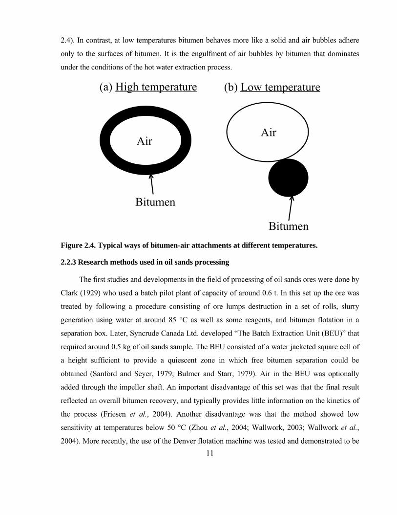
11
2.4). In contrast, at low temperatures bitumen behaves more like a solid and air bubbles adhere
only to the surfaces of bitumen. It is the engulfment of air bubbles by bitumen that dominates
under the conditions of the hot water extraction process.
Figure 2.4. Typical ways of bitumen-air attachments at different temperatures.
2.2.3 Research methods used in oil sands processing
The first studies and developments in the field of processing of oil sands ores were done by
Clark (1929) who used a batch pilot plant of capacity of around 0.6 t. In this set up the ore was
treated by following a procedure consisting of ore lumps destruction in a set of rolls, slurry
generation using water at around 85 °C as well as some reagents, and bitumen flotation in a
separation box. Later, Syncrude Canada Ltd. developed “The Batch Extraction Unit (BEU)” that
required around 0.5 kg of oil sands sample. The BEU consisted of a water jacketed square cell of
a height sufficient to provide a quiescent zone in which free bitumen separation could be
obtained (Sanford and Seyer, 1979; Bulmer and Starr, 1979). Air in the BEU was optionally
added through the impeller shaft. An important disadvantage of this set was that the final result
reflected an overall bitumen recovery, and typically provides little information on the kinetics of
the process (Friesen et al., 2004). Another disadvantage was that the method showed low
sensitivity at temperatures below 50 °C (Zhou et al., 2004; Wallwork, 2003; Wallwork et al.,
2004). More recently, the use of the Denver flotation machine was tested and demonstrated to be
Air
Bitumen
Air
Bitumen
(a) High temperature (b) Low temperature

12
a reliable way to obtain information on the kinetics of bitumen extraction (Kasongo et al., 2000;
Wallwork, 2003; Zhou et al., 2004). Nowadays, conditioning and bitumen liberation in
commercial operations are generally achieved using hydrotransport pipelines. With pipelining in
mind, Wallwork (2003) developed the so called “Laboratory Hydrotransport Extraction System
(LHES)”. This system was built using a heavy wall glass pipe of 17 mm internal diameter, and
25 mm external diameter. It included a 3 m pipe holding 4 L of slurry with the amount of oil
sands sample ranging between 1 to 3 kg (Wallwork et al., 2004). Some interesting features of this
system were the application of visualization techniques using high-speed cameras, and the
possibility of slurry aeration.
Several techniques and methodologies were also developed to study the fundamentals of
the surface chemistry phenomena occurring in oil sands processing. Dai and Chung (1995)
studied the bitumen-sand interaction using a very simple “bitumen pick up test”. In this test, a
bitumen-coated teflon plate (6 mm x 6 mm) was submerged into a solution containing a bed of
silica particles, and it was forced to move down against the sand bed allowing a contact time of 2
seconds. Afterward, the plate was removed from the solution and the amount of particles that
adhered to the bitumen layer was used as a parameter to evaluate the bitumen-sand interactions.
A high surface coverage with sand particles was interpreted as the result of high attractive forces
between bitumen and sand. Basu et al. (1996, 1998a, 1998b, 1998c, 2004) developed a technique
to measure the dynamic and static contact angles of bitumen on a glass surface under different
conditions of temperature and pH. This technique simulated the process of bitumen liberation
from sand surfaces, with the dynamic contact angle representing the bitumen liberation kinetics,
and the static contact angle the equilibrium conditions.
The bitumen extraction process is mainly controlled by the interfacial phenomena taking
place between bitumen, solid, and air bubble surfaces (Masliyah et al., 2004). For this reason, the
correct measurement and understanding of the electrokinetic properties of the components of the
oil sands ores is essential. The use of zeta potential measurements in this field has been widely
documented (Schramm and Smith, 1985; Dai and Chung, 1995; Veeramasuneni et al., 1996;
Zhou et al., 1999; Kasongo et al., 2000; Liu et al., 2002; Liu et al., 2003; Schramm et al., 2003;
Liu et al., 2004a; Liu et al., 2004b; Kasongo, 2006; Long et al., 2007). Liu et al. (2002)
developed a technique to investigate the bitumen-clay interactions by using measurements of zeta

13
potential distributions. This technique was based on the fact that for a suspension of a single
component (e.g., clay or bitumen), the zeta potential distributions displayed a single modal
pattern. However, for a suspension of two components the zeta potential distributions showed
either one or two distribution peaks, depending on whether the components interact with each
other or not. Another technique that was used to study the interaction forces existing between two
surfaces was the Atomic Force Microscopy (AFM) (Ravinovich and Yoon, 1994;
Veeramasuneni et al., 1996). This method was successfully applied to study the characteristics of
the repulsive and adhesive forces existing between bitumen and silica, and bitumen and clays
under different physicochemical conditions (Liu et al., 2003; Liu et al., 2004a; Liu et al., 2004b;
Liu et al., 2005; Kasongo, 2006; Drelich et al., 2007).
Some advances were also made in order to measure the rheology of oil sands slurries.
Gutierrez and Pawlik (2012) studied the rheology of artificial mixtures of bitumen with fine
quartz under different physicochemical conditions using a Haake Rotovisco VT550 rotational
viscometer. One important result obtained from that work suggested that there was a correlation
bitumen liberation and slurry rheology.
2.3 Effect of different variables on oil sands processing
The performance of the process of bitumen extraction from oil sands ores depends on
different process variables that can be classified into three main groups, i.e., ore properties, water
chemistry, and operating conditions (Table 2.1). Extensive research was done in order to
recognize and clarify the involved mechanisms (Clark, 1929, 1944, 1950, 1966; Clark and
Pasternack, 1932; Sanford and Seyer, 1979; Basu et al., 1996, 1998a, 1998b, 1998c, 2004; Dai
and Chung, 1995, 1996; Wallwork, 2003; Wallwork et al., 2003; Wallwork et al. 2004; Masliyah
et al., 2004; Long et al., 2007). It is noteworthy that almost all the variables presented in Table
2.1 affect the rheological behavior of the oil sands slurries in some way. For example, it was
shown that the combined action of pH and temperature governs the rheological behavior of
slurries prepared with artificial quartz-bitumen mixtures (Gutierrez and Pawlik, 2012). Moreover
the presence of monovalent and especially divalent cations was also shown to affect the surface
chemistry and rheology of these slurries (Gutierrez, 2009).

14
Table 2.1. Variables that affect the efficiency of the process of bitumen extraction from oil sands ores.
Ore Properties Water Chemistry Operating Conditions
Bitumen grade pH Temperature
Fines content Presence, valence and concentrations of ions
Mechanical mixing and residence time
Type of fines Presence and concentrations of
surfactants Slurry density
Mineralogy of sand and fines Presence and concentrations of
carbonates Aeration
Weathering of ores Presence and concentrations of
dispersants and polymers Bubble size
2.3.1 Effect of ore properties
Oil sands ores can be classified as “good processing ores” or “poor processing ores”
depending on their bitumen and fines contents (Zhou et al., 2000). The negative effect of high
levels of fines (-44 m) in the sand fraction on the process of bitumen extraction was previously
reported by several authors (Clark, 1944; Clark, 1950; Clark 1966; Liu et al., 2002; Liu et al.,
2004a; Tu et al., 2004; Kasongo 2006). It was found that the presence of high amounts of fines,
and ultra-fines (- 3 m) was in general associated with low bitumen grade ores (Tu et al., 2004;
Clark, 1950; Clark 1966), and that there was a direct relationship between the fines and ultra-
fines contents (Sanford, 1983). Other studies showed that fines extracted from poor processing
ores were more hydrophobic than those from good processing ores, which was associated with
the presence of products of degradation and weathering of the ores (Bensebaa et al., 2000; Sparks
et al., 2003; Liu et al., 2004a; Dang-Vu et al., 2009). These results were supported by
measurements of carbon contents in the ultra-fine fractions with higher carbon levels in fines
from poor processing ores (Tu et al., 2004). If fines are hydrophobic, they tend to adsorb on the
bitumen droplets reducing their hydrophobicity, and consequently lowering bitumen extraction as
well as bitumen liberation. These results are in agreement with those obtained by Liu et al.
(2004a) who studied the interactions between bitumen and fines extracted from good and poor
processing ores through AFM. These researchers found that the measured long range forces
between bitumen and fines from good ores could be described by the classical DLVO theory,
indicating that the electric double layer forces controlled the interfacial interactions between

15
these two components. In contrast, the study of interactions between bitumen and fines from poor
processing revealed that the DLVO theory required the introduction of an expression for
attractive hydrophobic forces to reasonably explain the experimental data. The effect of the ores
properties on the bitumen extraction from oil sands ores was also studied by Zhou et al. (2000)
using a Denver flotation machine. These researchers found that the kinetics of bitumen extraction
was significantly faster for good processing ores compared to that for poor processing ores. They
showed that for good processing ores more than 90 % of the bitumen could be floated within the
first 5 min, with the flotation rate constants being around 0.57 min–1. In contrast, flotation
experiments on poor processing ores showed that bitumen recovery was only around 20 % after
10 min with flotation rate constants being around 0.02 min–1. These differences in the bitumen
extractabilities between good and poor processing ores were also well documented by other
authors using the BEU and LHES methodologies (Sanford, 1983; Wallwork et al., 2003;
Wallwork et al., 2004).
2.3.2 Effect of water chemistry
The physicochemical characteristics of the water used in the process of bitumen extraction
are recognized as key for achieving good process performance. Specifically, the alkalinity and
presence of polyvalent cations were identified since the beginning of the research in this field
(Clark, 1929; Clark and Pasternack, 1932; Clark, 1944, Sanford and Seyer, 1979).
Dai and Chung (1995) showed that the zeta potential of bitumen and silica displayed
similar profiles with negative values over a wide range of pH (2-10), and isoelectric points of 3
and 2, respectively. Takamura (1985) proposed that the surface charge existing at the
bitumen/water interface could be explained by the dissociation of carboxyl and other acidic
groups naturally present in the bitumen component. This researcher based his conclusions on
experimental results of the predicted, and measured electrophoretic mobilities of bitumen drops
in aqueous electrolyte solutions. The theory offered by Takamura (1985) predicted that the
dissociation of carboxyl groups at the bitumen/water interface strongly depended on the
electrolyte concentration and pH of the aqueous solution according to Equation 2.1.
⇔ 2.1
16
The conclusions drawn by Takamura (1985) agreed with the results obtained by Sanford
and Seyer (1979) who showed a reduction of the surface tension and an increase of the organics
content in the secondary tailings as the pH of that stream increased. These results indicated a
relationship between the concentration of surfactants released from the bitumen phase to the
water phase, and the addition of NaOH. Accordingly, if the concentration of surfactants in the
water phase increases the bitumen/water interfacial tension decreases, and the process of
displacement of bitumen from the sand surfaces is enhanced (Basu et al., 1996; Schramm and
Smith, 1985, 1987a, 1987b, 1987c). It has to be noted that the beneficial effect of NaOH depends
on the stage of the process at which this reagent is added. Sanford (1983), Dai and Chung (1996),
and Kasongo (2006) showed that the positive effect of NaOH was only achieved when it was
added in the conditioning stage, before bitumen flotation, so that some reaction time was
allowed.
Dai and Chung (1995) reported strong adhesive interactions between bitumen and silica at
pH values below 7.0. Basu et al. (1996) found that the static contact angle of bitumen on glass
(measured across the bitumen phase) increased with pH supporting the idea that the bitumen
liberation from sand grains surfaces could be enhanced at high pH. However, these researchers
showed that the effect of pH on the kinetics response of the dynamic contact angle was minor
which suggested that bitumen liberation was not strongly affected by pH. Basu et al. (1998b)
reported that the changes in dynamic and static contact angles obtained as a result of the increase
in pH were minor when bitumen was extracted from poor processing ores, which correlated with
the difficulties in treating poor processing ores even at high pH values. Liu et al. (2003) used
AFM to study the interactions between bitumen and silica. These researchers showed that
repulsive forces between these components increased with pH, while the adhesive forces
decreased. This pH dependence was explained by the dissociation of cationic/anionic surfactants
at the bitumen/water interface. At low pH, cationic surfactants on the bitumen surface are
protonated to generate cationic sites (RNH3+) that interact with the OH- groups existing on the
silica surface, generating strong adhesive forces. In contrast, at high pH anionic surfactants
(RCOO- and ROSO3-) dominate the bitumen surface charge and forces between bitumen and
silica are repulsive. Figure 2.5 shows the results of AFM measurements obtained by Liu et al.,
2005 for the bitumen-silica system.

17
Figure 2.5. Repulsive (positive values) and adhesive forces (insert) between bitumen-silica surfaces as a function of separation distance and pH (Liu et al., 2003. With permission).
Liu et al. (2005) reported a Hamaker constant of attractive van der Waals interactions
between two bitumen surfaces in water of 2.8x10⁻²¹ J. This value is actually lower than the
Hamaker constant for quartz particles of 5x10-21 J (Franks, 2002). AFM results obtained by the
same researchers showed that the coagulation-dispersion of the bitumen-silica system could only
be properly described if the additional attractive hydrophobic forces were included in the total
force balance. These researchers characterized the hydrophobic forces using a constant of the
order of 10-19 J for the attractive forces between bitumen surfaces. According to this result the
hydrophobic forces existing between bitumen surfaces are much stronger than those explained by
the van der Waals forces. In other words, if pure particles of sand were coated with bitumen,
attractive forces between bitumen-coated particles should be stronger compared to interactions
between the pure quartz particles free of bitumen. Bitumen is also strongly hydrophobic under
neutral and weakly alkaline conditions with contact angles of water sessile drops on the order of
90 degrees, while silica is highly hydrophilic, a fact that certainly aids in bitumen-air attachment
and bitumen extraction from oil sands ores. The viscosity of oil sands slurries should be reduced

18
as bitumen is liberated from the surfaces of the sand grains. Gutierrez and Pawlik (2012) reported
a direct correlation between the bitumen content and the viscosity of synthetic oil sands slurries.
The viscosity of such slurries significantly increased as the amount of bitumen increased. These
researchers also found that the viscosity of these slurries significantly decreased with the increase
of pH which was explained by the increase of bitumen liberation achieved at high pH. This result
was confirmed by visual observations showing a higher amount of free bitumen on the slurry
surface as the pH was increased.
The presence of dissolved ions in the aqueous phase has a detrimental effect on bitumen
extractability. Specifically, the effects of sodium and potassium have been documented
(Takamura and Wallace, 1988; Kasongo, 2006; Basu et al., 1998c; Wallace et al., 2004; Liu et
al., 2003, 2004a, 2004b, 2005). Bivalent cations such as calcium and magnesium are also known
to have a negative effect on oil sands processing (Masliyah et al., 2004; Liu et al., 2002; Liu et
al., 2003; Kasongo, 2006; Liu et al., 2004b; Basu et al., 2004; Liu et al., 2005).
2.3.3 Effect of operating conditions
The control of temperature in oil sands processing was recognized as a very important
factor since early stages of development in this field (Clark, 1929, 1932, 1950, 1966). The use of
high temperature is critical to achieving high bitumen liberation (Wallwork, 2003; Wallwork et
al., 2004). In addition, it was also reported that the repulsive forces existing between bitumen and
silica increase with temperature, and at the same time the adhesive forces decrease which
improves bitumen extraction (Liu et al., 2002; Dai and Chung, 1995). As was previously
explained, temperature also affects the mode of bitumen-air contact. Zhou et al. (2004) found
that for good processing ores the kinetics of bitumen extraction strongly improved when
temperature was increased up to 50 °C, with no additional improvements obtained at higher
temperatures. Basu et al. (1996, 2004) showed that the rate of change of the dynamic contact
angle was much higher at high temperature and proposed that this result could be explained by
the reduction in bitumen viscosity. Wallwork (2003) also mentioned some undesired effects of
using high temperatures such as high levels of water and solids contents in the bitumen froth due
to the reduction of the overall viscosity.
19
Regarding to the effect of mechanical energy on oil sands processing, Kasongo (2006)
showed that bitumen recovery increased with agitation. Sanford (1983) showed that slime
coatings could also be reduced at high mixing energies, and that the effects of some surfactants
could be improved in this case as well. Sanders et al. (2007) found improvements in bitumen
extractability when the slurries were transported at high velocities. Some negatives effects were
also observed, especially in the treatment of poor processing ores for which excessive
mechanical agitation could lead to high levels of clays dispersion which may be detrimental to
bitumen extractability.
Slurry density has also been reported as a variable that affects bitumen extraction (Sanford,
1983; Wallace et al., 2004). Zhou et al. (2004) for example showed that bitumen recovery due to
true bitumen-air attachment increased with the reduction of the ore-to-water ratio. These authors
proposed that suitable dilution of oil sands slurries could be a viable way to improve the
efficiency of bitumen-air attachment, although excessive dilution also limits the capacity of
process equipment.
Oil sands slurries are aerated in order to generate aggregates of liberated bitumen droplets
and air bubbles (Liu et al., 2004b). However, it is becoming more common that additional air is
supplied into the hydrotransport pipeline in order to improve bitumen extraction (Wallwork et
al., 2004). Zhou et al. (2004) showed that at the same volume of air supplied to the system
bitumen recovery was much higher using continuous aeration than using staged-aeration.
Wallwork et al. (2004) showed for processing of poor ores that the final bitumen recovery
increased from 15 to 60 %, and the kinetics of bitumen liberation improved when external air
was supplied to the slurry.
Clark (1944) correlated the size of the bitumen droplets generated during the stage of ore
conditioning, and bitumen extraction showing that high recoveries could be obtained at droplet
sizes of around 200 m. Liu et al. (2005) argued that the process of aeration of bitumen and
bitumen flotation are affected by the size of bitumen droplets in the context of attachment
efficiency, with the size of bitumen droplets depending on coagulation and coalescence
phenomena.

20
2.4 Oxidation of oil sands
The dissociation of carboxyl groups at the bitumen-water interface depends on the
electrolyte concentration and pH with more dissociation at higher pH. Sanford and Seyer (1979)
found that at high pH the surface tension of the secondary tailings decreases, and the organics
content increases indicating a connection between the amounts of surfactants released into water
and the addition of NaOH. Extensive work was carried out by Schramm et al. (1984a, 1984b)
and Schramm and Smith (1985, 1987a, 1987b, 1987c) in order to quantify the free concentration
of surfactants in the liquid phase of oil sand slurries, and to study the effects of these surfactants
on the performance of the hot water extraction process. Schramm et al. (1984b) showed that
there was a single equilibrium concentration of free carboxylate surfactants, on the order of 1.2 x
10-4 N, at which bitumen recovery reached a maximum. The role of these natural surfactants is to
increase the negative charges at the oil-solution, and solid-solution interfaces with the oil/solution
interface displaying maximum electrophoretic mobility at the point of maximum efficiency of the
hot-water extraction process as explained by Schramm and Smith (1985). In this case these
researchers proposed that dispersion of air bubbles in the bitumen droplets is stabilized by the
action of the surfactants which enhances bitumen flotation. Schramm and Smith (1987a)
distinguished two types of surfactants, i.e., carboxylate surfactants and sulfate/sulfonate
surfactants. Carboxylate surfactants promote high bitumen recoveries near the optimum
concentration regardless of the concentration of sulfate/sulfonate surfactants. On the other hand
sulfate/sulfonate surfactants improve bitumen flotation when their solution concentrations are
near the optimum, and only if the carboxylate surfactant concentrations in solutions are very low
or zero.
The presence of surfactants in solution is affected by the degree of aging of the oil sands
ores (Mikula et al., 2008). Aging is a phenomenon that is known to deteriorate the extractability
of bitumen from oil sands (Mikula et al., 2003; Schramm and Smith, 1987b; Schramm and
Smith, 1987c; Charrie-Duhaut et al., 2000; Ignasiak et al., 1985). Aging in oil sands occurs when
bitumen suffers different types of alteration/degradation processes, such as dehydration,
oxidation of inorganics, oxidation of bitumen, loss of light hydrocarbons, water washing,
evaporation, biodegradation, and abiotic oxidation (Schramm and Smith, 1987b; Charrie-Duhaut
et al., 2000). Mikula et al. (2008) proposed that there was a partition of surfactants between the

21
aqueous and bitumen phase, and that achieving optimum recovery was not a result of the amount
of surfactants in the water phase but a consequence of the process of removal of surfactants from
the bitumen phase. These researchers showed that aged ores were rich in surfactants concentrated
in the bitumen phase, contributing to low bitumen recovery and poor froth quality. The addition
of NaOH promotes the transfer of surfactants from bitumen to water. These observations agreed
with observations made by other authors (Schramm and Smith, 1987b; Schramm and Smith,
1987c; Schramm and Smith, 1985) who found that the free concentration of surfactants in
solution decreased with ore aging, increasing the consumption of NaOH necessary to reach the
optimum surfactant concentration in the water phase. Free concentration of surfactants also
decreases as the ore grade decreases (Schramm and Smith, 1985). It was shown that during aging
there are chemical reactions that affect the source of carboxylate surfactants and/or that aging
generates species that consume NaOH (Schramm and Smith, 1987b).
Several authors detected, isolated and characterized what was called
toluene/dichloromethane insoluble organic matter (IOM) present in oil sands ores and tailings
(Charrie-Duhaut et al., 2000; Majid et al., 2000a; Majid et al., 2000b; Majid and Sparks, 1996;
Kotlyar et al., 1988; Kessick, 1979; Majid and Ripmeester, 1990; Majid et al., 1991; Majid et al.,
1992; Ignasiak et al., 1985; Kotlyar et al., 1990; Kotlyar et al., 1985). Most of the IOM consists
of humic matter, mainly humic acids (Kotlyar et al., 1988), and non-humic matter formed
primarily by organometallic compounds (Majid et al., 2000a). The presence of this IOM is
related to poor bitumen extraction, and it is in direct relationship with the degree of aging of the
ores (Ignasiak et al., 1985). The incorporation of oxygen functionalities takes place during the
process of aging, transforming organic molecules of bitumen into more hydrophilic humic-like
substances (Charrie-Duhaut et al., 2000). It was shown that most of the toluene/dichloromethane
insoluble organic matter concentrates in the fines fraction of the solids (Ignasiak et al., 1985;
Majid and Sparks, 1996; Majid et al., 1991). An important characteristic of the humic acids
extracted from oil sand ores or tailings is their similarity to those extracted from coal, specifically
to those obtained from coals of ranks higher than lignite. This characteristic was verified by
different authors (Kotlyar et al., 1988; Majid and Ripmeester, 1990; Majid et al., 1991; Majid et
al., 1992; Kotlyar et al., 1990) based on data of aromaticity, elemental analysis, and FTIR spectra
of the humic acids samples.

22
2.5 Interactions of humic acids and their effect on rheology of suspensions
Jones and Bryan (1998) explained that the organic matter in the environment (soils,
sediments and natural waters) can be classified into non-humic and humic substances. Proteins,
polysaccharides, nucleic acids, sugars, and amino acids can be listed among the non-humic
material. Humic substances are naturally occurring organic colloidal particles composed by
complex anionic macromolecules, yellow to black in appearance, acidic, consisting of carbon,
oxygen, hydrogen and lower amounts of nitrogen, phosphorous and sulphur. Humic substances
are very widespread in the environment representing a high percentage (70%) of the soil
composition, and can be categorized into fulvic acids, humic acids and humins (Jones and Bryan,
1998). Fulvic acids are soluble in water under all pH conditions, humic acids are soluble at pH
values above 2, and humins are always insoluble. Of these three types of humic substances,
humic acids are the most relevant products of the process of degradation of oil sands ores
(Kotlyar et al., 1988), and the analysis presented in the following paragraphs is focused on these
types of molecules.
As was previously explained humic acids are insoluble at pH below 2, and can be
precipitated from such strongly acidic solutions. When they are extracted using alkali solutions
they are dark brown to black in color. Under the pH conditions of most natural waters, they are
negatively charged (Wong and Laskowski, 1984), exhibiting properties characteristic of colloidal
particles in acidic conditions (Jones and Bryan, 1998). The alkali soluble humic acids can also be
precipitated by charge neutralization using cationic surfactants (Zouboulis et al., 2003; Gamboa
and Olea, 2006). They are also capable of complexing with metal ions (Jones and Bryan, 1998).
The most popular techniques used to extract humic acids from aquatic systems are coagulation
and precipitation (Zouboulis et al., 2003).
During the formation of humic acids some polymer segments generate carboxylic acid
groups, while other segments remain unaltered with the latter displaying more hydrophobicity
than the carboxylated segments (Gamboa and Olea, 2006). As a result, humic acid molecules
display hydrophilic and hydrophobic moieties in their chemical structure. Because of this
characteristic, humic acids have the ability to interact with other molecules by electrostatic and/or
hydrophobic interactions (Gamboa and Olea, 2006). This dual hydrophilic-hydrophobic structure
also imparts weak surface activity to these anionic polyelectrolytes. Terashimaa et al. (2004)

23
studied the influence of pH on the surface activity of humic acids using surface tension
measurement, and found that micelle-like aggregation of the humic acids molecules and
interfacial adsorption of humic acids were significantly enhanced in the acidic region. Gamboa
and Olea (2006) studied the surface properties of aqueous solutions of humic acids mixed with
some cationic surfactants, and found that the addition of small quantities of cationic surfactants
induced significant changes on the surface properties of humic acids resulting from the
generation of micelle-like structures produced below the respective critical micelle
concentrations.
Due to their complex and heterogenous nature and the presence of various types of
functional groups, humic acids are capable of interacting with a wide range minerals (Fairhurst
and Warwick, 1998; Jones and Bryan, 1998). Adsorption of humic acids to kaolinite, which is the
main component of the fines fraction in the oil sands ores, depends on pH, ionic strength as well
as on humic acids concentration. The anisotropic nature of kaolinite with negatively charged
faces and positively charged edges at pH values below 6-7 enhances the humic acids adsorption
through adsorption on the kaolinite edges at low pH, cationic bridging in the presence of cations,
and hydrophobic adsorption of uncharged parts of humic molecules. Elfarissi and Pefferkorn
(2000) studied the interactions between kaolinite and humic acids in the presence of aluminium
ions, and showed that the adsorption of non complexed humic acids was well explained by the
interactions between positive sites of the kaolinite, and negative groups of the humic acids.
Fairhurst and Warwick (1998) studied the adsorption of humic acids on minerals such as
boehmite and goethite and found that humic acids readily adsorbed onto the minerals with the
extent of adsorption decreasing with increasing pH. Furthermore, they found that humic acids
made more negative the zeta potential of the minerals at all concentrations and pH values.
Tipping and Higgins (1982) studied the stability of hematite in the presence of humic acids and
showed that humic acids enhanced the colloid stability of the haematite particles due to steric
stabilisation.
Wong and Laskowski (1984) investigated the effect of humic acids on the surface
properties of graphite. They found that adsorption of humic acids on graphite made the graphite
particles more negatively charged and more hydrophilic. Laskowski et al. (1986) studied the
effect of humic acids on coal flotation, and found that the addition of humic acids considerably
24
reduced the floatability of coal. These researchers also showed that both coal particles, and
kerosene droplets become more negatively charged in the presence of humic acids, and that this
effect was stronger in acidic pH. These authors observed that the depression of coal floatability
could be reversed by a second addition of oily collector and frother after some time of
conditioning. Liu and Laskowski (1988) studied the effect of humic acids on coal flotation at
different pH values showing that humic acids added to hydrophobic coal slurries depressed
floatability only at low values of pH, and that there was no effect in the alkaline range. They also
showed from contact angle measurements that humic acids rendered coal surfaces hydrophilic
only in the acidic pH range. This result agreed with their measurements of humic acids
adsorption that showed that humic acids adsorbed on coal predominantly in the acidic pH range.
Another point of view was given by Firth and Nicol (1981) who proposed that the depression of
floatability of hydrophobic coal could be explained by the adsorption of humic acids on clays
that reduced the availability of collector for coal particles, inhibiting coal flotation.
Pawlik et al. (1997) studied the effect of humic acids on the rheology of coal-water slurries
and found that coal-water slurries of hydrophobic coals exhibited high yield stresses and apparent
viscosities. On the other hand, slurries of hydrophilic coal displayed much lower yield stresses,
and viscosities. These authors attributed the high aggregation observed for slurries of
hydrophobic coal to the hydrophobic forces involved, concluding that the yield stress of these
slurries was proportional to the wettability of the coal. The low viscosities and yield stresses
found for slurries of hydrophilic coals were explained by the high repulsive forces due to the
negative surfaces charges of these hydrophilic coal particles. These researchers also showed that
the addition of humic acids changed the surface properties of the hydrophobic bituminous coals.
Hydrophobic bituminous coals became hydrophilic and more negatively charged when humic
acids were added resembling the surface properties of a lower rank or oxidized coal. The addition
of humic acids to slurries prepared with bituminous coals reduced the yield stresses, and apparent
viscosities. This effect was not observed in experiments with slurries of hydrophilic coal, because
in this situation the coal surfaces were already oxidized and any additional increase of the
negative charge of coal was insignificant. Pawlik et al. (2004) studied the effect of
hydrophobicity of coal on the aggregation of fine particles in concentrated coal-water
suspensions using steady-state rheological measurements. They observed that hydrophobic coal

25
particles aggregated over a wide pH range producing slurries with high yield stresses. As the
degree of coal oxidation increased, the coal particles became more hydrophilic, and the yield
stress values decreased to much lower values. Their results showed that coal aggregation and the
rheological behavior of coal-water slurries were strongly affected by wettability of coal particles.
It has to be noted that the degree of oxidation of coal can be measured using the alkali
extraction test developed by Lowenhaupt and Gray (1980). In this test, a given amount of ground
coal is boiled in a solution of NaOH so that the oxidized coal components, predominantly acidic
in nature (including humic acids) dissolve in the alkaline solution producing a tea-like color.
Then the extract solution is tested for light transmittance using a spectrophotometer. The
transmittance of the tested solution decreases with increasing coal oxidation. These authors found
that the alkali-extraction test correlated very well with the degree of coal oxidation determined
independently by coal petrography.
2.6 Hydrophobic interactions
From the previous discussion it is quite evident that hydrophobic interactions play an
important role in the surface chemistry and rheological behavior of suspensions of hydrophobic
particles. Hydrophobic attractive interactions are in general stronger than van der Waals forces
(Israelachvili and Pashley, 1984). Liu et al. (2005) reported the importance of these types of
interactions in the aggregation of bitumen and silica. Israelachvili and Pashley (1984) studied
hydrophobic interactions existing between two hydrophobic surfaces of mica coated with a
cationic surfactant. These authors found that for separation distances between these two surfaces
of 0-10 nm the hydrophobic forces could be described by the exponential function illustrated in
Equation 2.2.
= 2.2
Where FH is the magnitude of the hydrophobic force, R is the curvature of the mica
surfaces, C is a constant equal to 0.14±0.02 Nm-1, D0 is the decay length equal to 1.0±0.1 nm,
and D is the distance between the two mica surfaces. These authors found that van der Waals

26
attractions forces became comparable to hydrophobic interactions only at separation distances
above 10 nm, and that hydrophobic interactions acted over a longer range. Similar results were
obtained from measurements on the surfaces of artificially hydrophobicized mica performed by
Claesson et al. (1986). These researchers showed that an additional force was observed at
distances below 25 nm. These researchers also proposed a mechanism that explained the long
range hydrophobic forces based on surface-induced perturbations of the dynamic solvent
structure. Yoon et al. (1997) observed long-range hydrophobic forces with decay lengths of the
order of 2-32 nm, and proposed a double exponential function to describe the decay of
hydrophobic forces over large separation distances as shown in Equation 2.3
= 2.3
Where C1 and C2 are related to the interfacial tensions at the solid/liquid interface, and D1
and D2 are the decay lengths. Claesson et al. (1986) proposed a power law equation to quantify
hydrophobic forces as illustrated in Equation 2.4.
= 2.4
Where K is the hydrophobic force constant. Yoon et al. (1997) proposed the model
expressed by Equation 2.5 to correlate the contact angle and the hydrophobic force constant K.
This correlation was developed using data obtained from results on hydrophobicized silica for
which the constant K was determined from direct force measurements using AFM.
cos Θ 2.5
Where a and b are constant, and is the contact angle.

27
Parker et al. (1994) suggested that the long-ranged hydrophobic attractions are created due
to the presence of submicroscopic gas bubbles creating bridges between the hydrophobic
surfaces. These authors supported this idea arguing that the observed insensitivity of their results
to salt concentrations up to 1 M was related to the fact that surface tension did not change
significantly in this range and that electrostatic forces do not play a role in the long range forces.
Besides, they found that the range of attraction increased with temperature, and explained that
this effect was due to the growth of bubbles size. Zhou et al. (1996) studied the effect of
degassing on the coagulation of fine hydrophobic coal, and artificially hydrophobicized silica.
Their results showed that after degassing attractive forces existing between these types of
particles decreased which agreed with the conclusions presented by Parker et al. (1994) and the
work published by Ishida et al. (2000). A very important fundamental conclusion presented by
Zhou et al. (1996) was that if the true hydrophobic forces between surfaces were to be evaluated,
the system should be degassed before the experiments.
2.7 Rheology
2.7.1 General definitions
Rheology is defined as the science of study of deformation and flow of matter (British
Standard Glossary of Rheological Terms, BS 5168: 1975, British Standards Institution, 1975). It
is also recognized as the branch of physics that deals with the mechanics of deformable bodies
(Van Wazer et al., 1963). Every time a material is subjected to a stress, it will deform and flow
according to some rheological pattern which is characterized by a relationship between the
applied stress and the degree of deformation resulting from the stress application.
Two types of materials can be distinguished based on the deformation characteristics, i.e.,
fluids and solids materials. A fluid can be defined as a material that displays a measurable
magnitude of deformation after the applied stress is removed from the body, while for an ideal
elastic solid no deformation is observed (Whorlow, 1980). Therefore, the deformation of a body
can be divided into reversible elastic deformation and irreversible deformation referred to as
flow. In the first case, the energy required to generate elastic deformation is recovered when the
material returns to its original shape, while in the second situation the energy is dissipated as

28
heat. As this thesis deals with the rheology of oil sands slurries (suspensions), the subsequent
analysis will be focused on the rheology of fluids.
Shear is a very important type of deformation as several rheological techniques rely on it in
order to obtain rheological data. Figure 2.6 shows a situation in which a given fluid deforms
under conditions of simple shear strain. This type of deformation is characterized by the
movement of successive layers of fluid in parallel planes relative to a reference layer, in such a
way that the displacement of a layer is proportional to its distance from the reference layer
(Whorlow, 1980). The reference layer in Figure 2.6 is the plane at zero velocity and the ratio dl/l
is called the shear strain ( ). The shear rate ( ) is the rate of change of shear strain (dl/l/dt)
established as a result of the applied shear stress, and is expressed in units of reciprocal seconds
(s-1). In the case of fluids the share rate is used to describe flow. The shear stress ( is expressed
in units of force per unit area (Pa-Pascal).
Figure 2.6. Schematic of simple shear strain. v=velocity (m/s), y=vertical position (m), l=gap between parallel plates (m), =shear stress (Pa).
A convenient and widely used way to represent the behavior of fluids is through a flow
curve which is the functional relationship between shear stress and shear rate (Whorlow, 1980;
Krieger and Maron, 1951). In the case of Newtonian fluids, the relationship between shear stress
and shear rate is linear from zero, with the slope of this straight-line referred to as the “viscosity
coefficient”. For non-Newtonian fluids this relationship is not a straight-line. The “apparent

29
viscosity” is defined as the ratio of the shear stress to the shear rate (Equation 2.6) with units of
Pascal-second (Pas). Apparent viscosity represents the viscosity at a given shear rate.
2.6
Experimental data of the shear stress and shear rate are obtained from rheological
measurements that are carried out using rheometers. Walters (1975) distinguished two main
objectives of rheological measurements. The first objective is to determine the behavior of non-
Newtonian fluids using simple rheometrical geometries so that a correlation between the fluid
properties and its rheological behavior can be obtained. The second objective is the prediction of
the flow behavior in complex flow situations using results from simple rheological tests, and with
the assistance of sophisticated mathematical methods. Three types of rheological measurements
can be distinguished (Whorlow, 1980; Utracki, 1988). In the first type, the fluid to be tested
flows steadily in the rheometer and measurements of the corresponding shear stress and shear
rates are done. In the second category, the shear rate is measured as a function of time under the
action of a constant shear stress, or changes in the shear stress (decay/growth) are measured
under a constant shear rate. The third type of rheological measurement deals with tests in which
oscillatory forces are applied, and the dynamic response of the system is obtained.
It is important to remark that the shear rate values obtained from typical rheological
measurements (concentric cylinders) are usually values corresponding to an apparent shear rate.
This situation arises from the fact that the shear rate values can be different depending on the
type of rheological technique utilized. Consequently, the experimental value of shear rate has to
be viewed as an approximation to its actual value. However, for simplicity in the rest of this
thesis the expression “shear rate” will be used.
2.7.2 Typical rheological responses
The most common relationships between shear stress and shear rate for mineral
suspensions are summarized in Figure 2.7. They can be categorized into two main groups, i.e.,

30
those flow curves displaying an initial shear stress, referred to as the yield stress, that have to be
overcome to produce deformation, and those without a yield stress.
The simplest type of behavior is described by the Newton’s law of viscosity. In this case
the relationship between shear stress and shear rate is a straight-line starting from zero, with the
slope of this line being the viscosity coefficient. Newtonian fluids are characterized by this sole
parameter which is independent of the shear rate and time. Examples of Newtonian behavior are
organic liquids of low molecular weight, water, aqueous solutions, liquid metals, and diluted
suspensions of spherical and non-interacting particles (Whorlow, 1980; Van Wazer et al., 1963;
Tadros, 1980).
Fluids that display a non-linear relationship between shear stress and shear rate are
collectively referred as non-Newtonian fluids. This is for example the case of shear thinning or
pseudoplastic fluids for which a time-independent decrease of viscosity is observed as the shear
rate increases. These fluids are the most common examples of solid-liquid suspensions exhibiting
non-Newtonian behavior (Cross, 1965; Boger, 1977). It was also observed that in general the
flow curve for pseudoplastic fluids is characterized by an initial region of constant viscosity at
very low shear rates, followed by an intermediate section where the apparent viscosity decreases
with shear rate, and ending with a second segment of constant viscosity values at very high shear
rates (Boger, 1977; Van Wazer et al., 1963). It is because of this distinctive profile that
pseudoplastic fluids are said to display a lower and upper part of Newtonian behavior (Boger,
1977). In contrast, shear thickening or dilatant materials are characterized by a time-independent
increase in apparent viscosity as shear rate is increased.
The second category of rheological response is typical of fluids for which a continuous
deformation is only observed after the applied shear stress exceeds a minimum stress value, i.e.,
the yield stress (Bingham, 1930; Lang and Rha, 1981; Nguyen and Boger, 1983). Among these
fluids the plastic or Bingham fluids can be distinguished for which a linear flow curve is
observed after yielding. In contrast, those fluids that display a non-linear flow curve after the
yield stress is overcome are called pseudoplastic with yield stress or shear thickening with yield
value (Van Wazer et al., 1963).

31
There are also several fluids that exhibit time-dependent effects, either reversible or
irreversible (Van Wazer et al., 1963; Cheng, 1986). One example is thixotropy that can be
defined as the continuous decrease of stress with time at steady shear rate, with a recovery of the
structure when flow stops (Utracki, 1988; Mewis, 1979). The phenomenon opposite to thixotropy
is called rheopexy. In the case of suspensions containing interacting solids particles, thixotropy is
in general explained by the rupture of interparticle bonds resulting from the shearing action
(Morgan, 1968), with the rate of rupture of these bonds being a time-dependent variable. Van
Wazer et al.(1963) suggested two methods for measuring thixotropy. The first method consisted
of measuring the up and down branches of the flow curve, while the second method involved the
measurement of the stress decay as a function of time at a given shear rate. Saunders (1961) used
the first method and measured the area of hysteresis of the flow curve of thixotropic fluids to
study the effect of thickening organic polymers on latex suspensions. This author showed that
thixotropy and plastic viscosity slightly increased with the increase of the thickener concentration
which could be related to the presence of interparticle bonds and agglomerates of particles. This
study also showed that a decrease of the latex particle size at constant thickener concentration
increased thixotropy, plastic viscosity, and yield stress. Mewis (1979) explained that thixotropy
could appear in a variety of systems and that its occurrence depends on the presence of a
reversibly variable structure. Cheng (1986) showed that the magnitude of the yield stress
depended on the time interval between consecutive measurements, revealing that the yield stress
can also be a time-dependent property. Cheng explained that in thixotropic fluids the yield stress
depends on the fluid structure, and as this structure changes with time the yield stress also
changes with time. Perhaps the most significant conclusion of the work by Cheng (1986) is that
the yield stress obtained from the equilibrium flow curve is the same as that for the fully built-up
structure only after a prolonged rest of the sample, and that in general, the static yield stress
measured after a long rest is much higher than the yield stress obtained from the equilibrium flow
curve.

32
Figure 2.7. Common relationships between shear stress and shear rate.
2.7.3 Flow curve modeling
Flow equations are mathematical models used to fit experimental rheological data obtained
from measurements on fluids displaying rheological patterns such as those described in the
previous section. Analysis and interpretation of the parameters and constants of these models can
be used to correlate the rheological behavior with the physical and chemical properties of the
studied fluids (Krieger and Maron, 1951; Green and Griskey, 1968a; Cross, 1965; Quemada,
1978). The correct selection of a flow equation should match the following criteria (Whorlow,
1980; Cross, 1965):
(a) The mathematical expression of the flow equation should be simple.
(b) The fitting to the experimental data should be accurate over a wide range of shear rate.
(c) The number of model parameters should be minimum.
(d) The parameters of the flow equation should be easily obtained, preferably through graphical
methods.
(e) The parameters should have a physical meaning.

33
(f) The flow equation should be generalized into a tensor form.
The flow of Newtonian fluids can be modeled by the Newton’s law of viscosity (Equation
2.7).
2.7
Where is the coefficient of viscosity. In the case of suspensions, Newtonian behavior is
in general observed at lower solids concentrations of the dispersed phase of less than 20 vol.%
(Krieger and Dougherty, 1959; Rutgers, 1962a; Rutgers, 1962b). Krieger and Maron (1951),
Maron et al. (1951), Maron and Madow (1953), Maron and Fok (1955), Maron and Levy-Pascal
(1955), and Saunders (1961) for example showed that suspensions of latex particles displayed
Newtonian behavior up to solids concentrations of 20-25 vol.%. Maron and Madow (1953) found
that in the range of 25 to 47 vol.% latex suspensions displayed Newtonian behavior only at low
shear rates, and non-Newtonian behavior at high shear rates, results that tend to agree with those
by Lewis and Nielsen (1968) who found that suspensions of glass particles of sizes ranging
between 5 and 105 m displayed Newtonian behavior up to solids concentrations of 45 vol.%.
Maron and Madow (1953) found that when the solids contents of latex suspensions were higher
than 47 vol.%, non-Newtonian behavior was observed over the whole range of shear rate.
The power-law or Ostwald-de Waele flow equation can be mathematically expressed by
Equation 2.8.
2.8
Where K is called the consistency parameter and n the power-law index. The constant K in
this model has units of Pasn and the power-law index n is dimensionless with its deviation from 1
being a measure of the degree of non-Newtonian behavior. For n equal 1, the model becomes the
Newton’s law of viscosity, for n greater than 1 the model describes a shear thickening behavior,
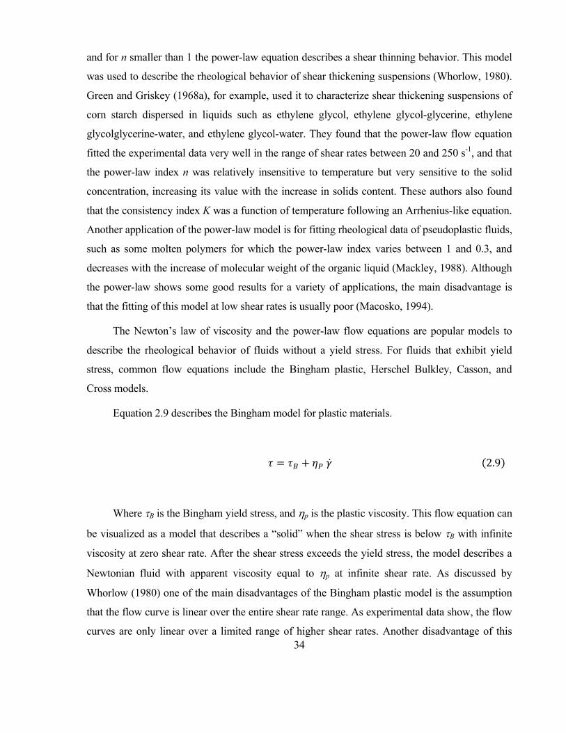
34
and for n smaller than 1 the power-law equation describes a shear thinning behavior. This model
was used to describe the rheological behavior of shear thickening suspensions (Whorlow, 1980).
Green and Griskey (1968a), for example, used it to characterize shear thickening suspensions of
corn starch dispersed in liquids such as ethylene glycol, ethylene glycol-glycerine, ethylene
glycolglycerine-water, and ethylene glycol-water. They found that the power-law flow equation
fitted the experimental data very well in the range of shear rates between 20 and 250 s-1, and that
the power-law index n was relatively insensitive to temperature but very sensitive to the solid
concentration, increasing its value with the increase in solids content. These authors also found
that the consistency index K was a function of temperature following an Arrhenius-like equation.
Another application of the power-law model is for fitting rheological data of pseudoplastic fluids,
such as some molten polymers for which the power-law index varies between 1 and 0.3, and
decreases with the increase of molecular weight of the organic liquid (Mackley, 1988). Although
the power-law shows some good results for a variety of applications, the main disadvantage is
that the fitting of this model at low shear rates is usually poor (Macosko, 1994).
The Newton’s law of viscosity and the power-law flow equations are popular models to
describe the rheological behavior of fluids without a yield stress. For fluids that exhibit yield
stress, common flow equations include the Bingham plastic, Herschel Bulkley, Casson, and
Cross models.
Equation 2.9 describes the Bingham model for plastic materials.
2.9
Where B is the Bingham yield stress, and p is the plastic viscosity. This flow equation can
be visualized as a model that describes a “solid” when the shear stress is below B with infinite
viscosity at zero shear rate. After the shear stress exceeds the yield stress, the model describes a
Newtonian fluid with apparent viscosity equal to p at infinite shear rate. As discussed by
Whorlow (1980) one of the main disadvantages of the Bingham plastic model is the assumption
that the flow curve is linear over the entire shear rate range. As experimental data show, the flow
curves are only linear over a limited range of higher shear rates. Another disadvantage of this

35
model is that when suspensions show time-dependency the yield stress cannot be clearly
identified which makes it difficult to fit the data using Equation 2.9. Regarding the determination
of the yield stress using the Bingham model, Nguyen and Boger (1983) showed that this
extrapolation procedure has to be taken with precautions, and that the value B should be taken
just as a model parameter but never as a material property. These authors proposed that the
Bingham model is more appropriate for high shear rates.
The Herschel-Bulkley flow equation (Herschel and Bulkley, 1926) illustrated in Equation
2.10 is a combination of the power-law and the Bingham plastic models. If the yield stress is zero
the equation assumes the expression of the power-law model and if the value of n is one, the
equation assumes the form of the Bingham plastic model.
2.10
Where B is the Herschel-Bulkley yield stress, and KHB and n are as described for the
power-law model. The presence of the parameter n in this flow equation provides one more
degree of freedom with respect to the Bingham model which is very helpful in obtaining a good
fitting of the rheological data in the low range of shear rates. Because of this characteristic, the
estimation of the yield stress using this model is considered to be more accurate than that with
the Bingham model. It was reported that the Bingham yield stress (B) can be up to 4-5 times
higher than that obtained from the Herschel-Bulkley model (Nguyen and Boger, 1983).
Casson (1959) proposed a two parameter flow equation that was developed assuming a
degree of particle aggregation in suspensions. This author assumed that particles in suspension
aggregate due to action of interparticle forces, forming linear chains of certain dimensions that
can be visualized as rigid rods. According to this theory, energy is dissipated as a result of the
motion of these rigid rods, and this energy dissipation is proportional to the dimensions of the
rods. Equation 2.11 shows the Casson model.
/ / / 2.11

36
Where 0 is the Casson yield stress and pl is the limiting viscosity at high shear rates. This
model has a more gradual transition in the low shear rate region than the Herschel-Bulkley model
and it was shown to be successful when fitting rheological data of blood and food products
(Macosko, 1994). The Casson model has some important advantages, i.e., the number of
parameters of this model is less than that for other flow equations, and every parameter has a
physical meaning.
Cross (1965) developed a flow equation assuming that the process of
aggregation/flocculation in suspensions involves groups of linked particles that create chains of
aggregates, with the size of these groups depending on the applied shear rate. At very high shear
rates the suspension becomes completely deflocculated. In this model, the rate of links rupture is
attributed to the shearing action and Brownian movement, while the rate of links creation is a
result of Brownian movement only. Considering all the previously mentioned assumption Cross
(1965) obtained Equation 2.12.
1 2.12
Where is the apparent viscosity, 0 is the apparent viscosity at zero shear rate,∞ is the
apparent viscosity at infinitely high shear rate, is the ratio of the kinetics constant of links
rupture by shearing (k1) to the kinetics constant related to rupture due to Brownian movement
(k0), and m is an empirical constant on the order of 2/3 for many pseudoplastic materials. A high
value of implies a relatively large shear dependent contribution to structural breakdown.
Barnes et al. (1989) analyzed the results of the applicability of the Cross model to rheological
data for polyacrylamide solutions (Boger, 1977), blood (Mills et al., 1980), aqueous latex
(Quemada, 1978), and aqueous solutions of xantham gum (Whitcomb and Macosko, 1978).
Macosko (1994) also gave some examples of the fitting of this model to experimental data
obtained from yogurt (De Kee et al, 1980), polystyrene-ethylacrylate latex spheres (Laun, 1988),
and polymer melt (Cox and Macosko, 1974).

37
Several other flow equations have been proposed to fit rheological data (Papanastasiou,
1987; Yasuda et al., 1981; Carreau 1972; Carreau, 1979a; Carreau, 1979b; Ree and Eyring 1955a
and 1955b; Ellis, 1929; Parzonka and Vocadlo, 1968) but they are less common in analyzing the
rheology of suspensions.
2.7.4 Rheometry
Rheometry is the science of measuring stress and deformation history on a fluid for which
the constitutive relation is unknown (Macosko, 1994). As was previously explained, rheological
measurements are done using rheometers. In the case of fluids, rheometers usually use the
concept of simple shear previously explained. Macosko (1994) classified shear rheometers into
two groups. The first group contains those rheometers for which the shearing action results from
the motion of two solid surfaces, one moving and one fixed (drag flow). Concentric cylinders,
cone and plate, sliding plates, and parallel disks are examples of these types of rheometers. The
second category is characterized by the use of pressure gradients in order to produce flow
(pressure driven flow). In this case the shearing action is generated by a pressure difference
between the entrance and the exit of the device, as in for example tube or capillary rheometers,
slit flow, and axial annulus devices.
Among the previously mentioned examples, tube/capillary and concentric cylinders
rheometers are the most popular (Krieger and Maron, 1951). In tube rheometers the flowrate (Q)
is measured as a function of the pressure gradient P/L along the tube. In concentric cylinder
rheometers one of the cylinders rotates at a given angular velocity , and the required torque T
needed to generate this angular velocity is determined. Then, from the corresponding
relationships between Q and P/L, and and T, and considering the geometrical dimensions of
the devices, the corresponding values of shear rate and shear stress can be calculated. Perhaps the
most important limitation of these two types of rheometers is the poor capability to study the
response of materials to large transient deformations, for which sliding surfaces were found to be
more advantageous (Dealy and Giacomin, 1988). A variety of other different types of
rheometers are described in the literature and very good reviews respect to this topic can be
found in Whorlow (1980), Van Wazer et al. (1963), Walters (1975), and Macosko (1994).

38
A description of the general assumptions and mathematical expressions necessary to
interpret the experimental rheological data obtained from measurements using concentric
cylinders rheometers as well as an explanation of the possible errors of measurements is given in
sections 2.7.4.1 and 2.7.4.2. The determination of flow curves using the infinite gap approach is
analyzed in section 2.7.4.3.
2.7.4.1 Concentric cylinder rheometers
Concentric cylinder rheometers are the most widely used commercial instruments to
measure the rheological properties of fluids (Macosko, 1994). One important advantage of this
type of device is that the rheological measurements can be followed for long periods of time
which allows gathering data to analyze time dependent effects (Van Wazer et al., 1963). In
addition to this, the use of concentric cylinders for which the gap existing between the two
cylinders is very small compared to the radius of the inner cylinder, makes it possible to
approximate the conditions of uniform shear rate across the gap, which is difficult to achieve
using other geometries. Some disadvantages of concentric cylinders were also brought out, such
as the presence of the Weissenberg (rod climbing) effect (Dealy and Giacomin, 1988) for high
viscosity liquids, sample loading and cleaning of the components of these rheometers can be
problematic too. Obtaining concentricity of the cylinders can also be complicated especially for
tests done at high temperature using cylinders of small gap. Viscous heating is also an issue for
high viscosity liquids and reproducibility of the tests may be worse than for tests with tube
rheometers (Whorlow, 1980).
Figure 2.8 (a) shows a horizontal section of a concentric cylinder rheometer consisting of
two solid surfaces, i.e., an inner cylinder of radius r1, and an outer cylinder of radius r2. The inner
cylinder is fixed, and the outer cylinder rotates at an angular velocity . The development of the
equations that correlate shear stress and shear rate requires some general assumptions (Whorlow,
1980; Van Wazer et al., 1963). The first assumption is that the flow is steady and laminar in the
annular section existing between the cylinders, with the fluid elements moving in circular
streamlines around a common axis at angular velocities r. The second assumption is that end
effects are negligible, condition that can be approximated by using cylinders of large height to
diameter ratios. Finally, inertia effects, and wall slip are also assumed to be negligible.

39
Considering all these assumptions, the torque T generated by the shearing action of a
cylindrical surface of height H, at a radius r from the axis of the cylinder is given by Equation
2.13.
2 2.13
Then, the shear stress on the inner and outer cylindrical surfaces can be calculated from
Equations 2.14 and 2.15.
2 2.14
2 2.15
Figure 2.8. (a) Cross-section, and (b) a fluid element in a concentric cylinder viscometer.
To fully describe rheological data, it is necessary to develop an expression for the shear
rate. The shear strain in a concentric cylinder rheometer can be obtained by analyzing the
schematic of the fluid element shown in Figure 2.8 (b). From the definition of simple shear strain
given in section 2.7.1 (Figure 2.6), the shear strain for the situation presented in Figure 2.8 (b) is
given by Equation 2.16 (Whorlow, 1980).

40
2.16
In the limit as dr tends to zero the shear rate can be expressed as in Equation 2.17.
2.17
The proper mathematical handling of Equations 2.13 and 2.17 leads to expressions for the
shear rate as a function of the geometrical constants, and the flow equations parameters for
different types of fluids.
The simplest case is when the gap existing in annular section between the inner and outer
cylinders (r2-r1) is very small compared to the radius of the inner cylinder (r1). In this condition
the shear stress and shear rate can be approximated using Equations 2.18 and 2.19 respectively.
2 2.18
Ω 2.19
Where ra is the average radius between r1 and r2.
For Newtonian suspensions, the expressions for the shear rate at both, the inner and outer
cylinders as a function of the angular velocity of the outer cylinder can be obtained by
manipulating Equations 2.7, 2.13, and 2.17. The resulting mathematical expressions are
illustrated in Equations 2.20 and 2.21.
2
Ω 2.20 2
Ω 2.21

41
In the case of power-law suspensions, the shear rates evaluated at the inner and outer
cylinders can be calculated using Equations 2.22 and 2.23 respectively.
2Ω
1
2.22 2Ω
1
2.23
Similar expressions can be developed for suspensions that follow the Bingham (Whorlow,
1980; Toorman, 1994), Casson (Joye, 2003), and Herschel-Bulkley flow equations (Kelessidis
and Maglione, 2008). Additional work was done by Krieger and Elrod (1953), Krieger and
Maron (1954), and Krieger (1968) in order to obtain general methods to estimate the correlation
between the shear rate and shear stress in concentric cylinder rheometers.
2.7.4.2 Errors of measurements in concentric cylinder rheometers
Whorlow (1980), Walters (1975), Van Wazer et al., (1963), and Klein (1992) mentioned
some important factors that can lead to erroneous results of rheological measurements in
concentric cylinder rheometers, i.e., end effects, turbulence, viscous heating, wall effects, particle
settling, and gap length to maximum particle size ratio.
End effects arise from the fact that the rheometers dimensions are finite, and also from the
difference between the shear stress exerted on the end of the bob and the shear stress on the
shearing surface. Some ways that are usually followed to reduce the influence of the end effects
are as follows (Van Wazer et al., 1963):
(a) To use a high bob length to bob diameter, or to reduce the area at the ends of the bob.
(b) To add a conical section to both ends of the bob, so that the contributions of the ends to
the total shear stress can be calculated and accounted.
(c) To create a space in the bottom of the bob so that air can be trapped into that space and
the torque can be minimized due to the fact that air displays a very low resistance to flow.
As was previously explained, the condition of laminar flow is assumed in order to obtain
expressions for the shear rate in concentric cylinder rheometers. Therefore, it is important to

42
make sure that this condition can actually be held during the rheological measurements. The
onset of turbulence in concentric cylinder rheometers can be estimated using the analysis
proposed by Taylor (1923). If the inner cylinder rotates, the critical Reynolds number at which
the onset of turbulence occurs can be determined by Equation 2.24 (Van Wazer et al., 1963).
41.3 2.24
Where vb is the tangential velocity of the moving part, is the slurry viscosity, and is the
density of the suspension. In contrast, if the outer cylinder rotates, the onset of turbulence occurs
at Reynolds numbers as high as 50,000. This increase in flow stability can be explained by the
stabilising action of the centrifugal forces in Couette flow that happens if the outer cylinder is
rotated (Van Wazer et al., 1963). Experimentally, the onset of turbulence can be detected from
the presence of a sharp and sudden increase in the shear stress which is a result of the increase in
energy dissipation resulting from turbulence flow.
For high viscosity fluids, a significant increase in the temperature of the sample can occur
during rheological measurements in concentric cylinders. This phenomenon arises from the fact
that the energy supplied to produce shearing results in heat dissipation, increasing the
temperature of the sample. This phenomenon may be significant and in some cases erroneous
conclusions can be drawn if it is not taken into account (Whorlow, 1980). For example, if the
increase in temperature is not considered as a factor during the experiments, a decrease in
viscosity with time could be interpreted as thixotropic behavior, while what actually caused the
decrease in viscosity was the increase in temperature.
In general, it is assumed that the tangential velocity of the bob is equal to that of the fluid
contacting it. However, in some cases such as concentrated suspensions, gels, and polymer
solutions, a low viscosity layer can develop near the cylindrical surface. In this case, a velocity
difference is observed between the bob and the fluid and a phenomenon called wall slip is
observed (Macosko, 1994; Whorlow, 1980). One method that is usually used to reduce this

43
slippage is to use grooved shearing surfaces. However, in some cases the size of the annular gap
becomes uncertain, especially for small gaps, when the surfaces of the inner and outer cylinders
are grooved.
Settling is another very important effect that has to be taken into account during the
experimental design of rheological experiments (Klein, 1992; Klein et al., 1995). For particles of
high specific gravity suspended in low viscosity suspensions, the rate of gravitational settling is
significant. In this situation, if the suspension is placed in the annular gap existing in between the
two concentric cylinders, settling will take place, and the solids concentration of the suspension
will vary along the vertical axis of the concentric cylinder rheometer. Consequently, the torque
measured on the moving cylinder will not represent the behavior of the overall suspension and
results will be erroneous. Klein (1992) designed an elongated concentric cylinder rheometer that
is based on the zone settling properties of mineral suspensions. As a low solids zone develops in
the top layers of the tested suspension as a result of particle settling, the rotating bob is positioned
at some depth within the suspension, in a zone of constant solids content. In this way, reliable
data can be collected before the low solids zone reaches the rotating bob.
Another factor that can affect the results is the dimensional relation between the gap length
and the size of the coarsest particle in the suspension. Van Wazer et al. (1963) proposed that the
gap of the annulus between the concentric cylinders should be at least 10 times larger than the
diameter of the largest particle in suspension so that particle trapping across the gap can be
avoided.
2.7.4.3 Infinite gap approach
Krieger and Maron (1952, 1953, 1954) and Krieger and Woods (1966) solved the basic
equation for coaxial rotational rheometers presented in Equation 2.25 for various sets of
boundary conditions.
Ω12 2.25

44
Where is the shear rate at the same point of measurement of the shear stress ,
and 1 and 2 are the shear stresses exerted on the inner and outer cylinders respectively. This is
a general expression valid for steady flow in rotational rheometers (Jacobsen, 1974). This
expression can be solved for the special case where a cylindrical bob rotates in an infinite cup
(Jacobsen, 1974). In this situation the shear stress on the cup () becomes zero in Equation 2.25
and the expression can be differentiated with respect to the shear stress on the bob (τ1) obtaining
Equation 2.26.
2 2.26
According to this expression the shear rate values can be obtained by evaluating the slope
of a graph of Ln() versus Ln(1). This equation assumes that there is complete shearing
occurring across the infinite gap between the bob and cup. This assumption apparently excludes
suspensions that display a yield stress for which volumes of fluids of zero shearing exist in the
gap. However, it can be shown (Jacobsen, 1974) that Equation 2.26 is still valid for suspensions
with a yield stress. In this situation the integration limits in the right hand of the Equation 2.25
are τ1 and 0 with the latter value being the yield stress. As the yield stress is a constant, the
derivative of the right hand of Equation 2.25 related to the upper limit of the integral is still zero,
and the result for fluids with and without yield stress is the same.
2.7.5 Micro-rheology of suspensions
The rheological behavior of suspensions of particles dispersed in a continuous medium
depends on the phenomena occurring at an inter-particle level which are called micro-rheological
effects. The prediction of the macroscopic suspension rheology from the description of the
behavior of the microscopic elements is the subject of micro-rheology (Goldsmith and Mason,
1962, 1967). Four types of micro-rheological effects can be distinguished, i.e., hydrodynamic,
granulo-viscous, electro-viscous, and aggregation (Klein, 1992). The hydrodynamic effects arise
firstly from the flow resistance generated as fluid moves around a particle, and secondly from the

45
squeezing of liquid that takes place as particles approach each other. The granulo-viscous effects
are related to physical interactions between particles such as particle impacts, inter-particle
friction, and particle packing. The electro-viscous effects arise from mutual interactions between
electrical double layers generated around the particles that form the suspension, with these
interactions affecting the magnitude of energy dissipation. Finally, the aggregation effects are
created by the action of attractive interparticle forces (van der Waals forces).
It is important to note that the electro-viscous and aggregation effects are important for
small particle sizes (< 20 m) with both effects being more significant at high solid contents.
However, when particles are suspended in very high viscosity liquids, particle-particle
interactions will be minimal and no long-range "structures" will be created (Metzner, 1985). The
relative importance of these micro-rheological effects depends on various properties of the
suspension that can be classified as physico-mechanical, i.e., solid content, density, shape, size
and size distribution of the particles, and physico-chemical variables, pH, ions, surfactants, other
chemicals (Klein, 1992).
2.7.6 Effect of particle size and particle size distribution on rheology of suspensions
Utraki (1988) summarized three reasons that explain the effect of particle size on rheology,
i.e., low mobility of liquid molecules adsorbed on the surface of small particles, contribution of
Brownian motion at small sizes, and effects of colloidal aggregation. Sweeny and Geckler (1954)
also mentioned the importance of electro-viscous effects. Brandenburg and Lagaly (1988)
studied the rheology of montmorillonite suspensions finding that the viscosity increased sharply
as particle size decreased below 0.6 m. Sweeny and Geckler (1954) found that the apparent
fluidity of suspensions of glass spheres dispersed in aqueous liquids decreased as the particle size
decreased. The same authors found that when the aqueous medium was replaced by a non-
aqueous ethylene tetrabromidediethylene glycol medium, no effect particle size effect was found
which can be explained by the lower extension or absence of the electrical double layer in
organic liquids. These researchers proposed that the effect of particle size on rheology arises
from electro-viscous effects, and from the presence of an adsorbed layer of fluid attached to the
particles surfaces, both effects being more relevant for small particle sizes, and promoting an
increase in the effective volume concentration.
46
Regarding the effect of particle size distribution, Sweeny and Geckler (1954) proposed that
the viscosity of suspensions for a given solids content decreases if blends of particles of varying
sizes are used instead of a single narrow size fraction. Similar results were reported by other
researchers (Luckham and Ukeje , 1999; Sweeny and Geckler, 1954; Boylu et al., 2004;
Rodriguez et al., 1992; Sengun and Probstein, 1989a-1989b; Probstein et al., 1994; Hoffman,
1992; Farris, 1968; Parkinson et al., 1970). Sweeny and Geckler (1954) explained that this
phenomenon is a result of the increase in the maximum packing fraction when polydisperse
systems are used. If particles of different sizes form a suspension, those of small sizes occupy the
void spaces created in between the larger particles increasing the maximum packing. Suspensions
of high maximum packing fractions display low viscosities (Utraki, 1988; Poslinski et al., 1988;
Wildemuth and Williams, 1984, 1985; Lewis and Nielsen, 1968; Hoffman, 1992). Metzner
(1985) also proposed an additional mechanism to explain the effect of particle size and particle
size distribution on the rheology of concentrated suspensions which has to do with the fact that
the presence of small particles in suspension improves the sliding of layers of particles of fast
motion against layers of particles of slow motion. The result is a reduction of viscosity.
Fidleris and Whitmore (1961) showed that when the size ratio of small to large particles
was 0.1 or less the large sphere moved through the suspension of fines as if it was moving
through a liquid of the same viscosity and density as the suspension of fine particles. On the other
hand, when the size ratio was higher than 0.1 the motion of the sphere followed a zig-zag random
path indicating some interactions between coarse and small particles. Using this concept Farris
(1968) developed a theory in which the viscosity of a multimodal suspension can be calculated
from the uni-modal viscosity data. The theory considers that when solid particles or fillers are
added to a liquid of viscosity 0, the viscosity of the liquid is increased to a new value f. This
author defined a stiffening factor H() as the relative viscosity of an uni-modal system to that of
the liquid alone as expressed in Equation 2.27.
∙∙∙ 2.27

47
Farris (1968) used this theory to calculate the viscosity of multimodal suspensions
obtaining a very good fitting to the experimental data.
2.7.7 Yield stress determination
2.7.7.1 General considerations
Several definitions of the yield stress were proposed with some significant physical
differences. Some authors (Bingham, 1930; Lang and Rha, 1981; Nguyen and Boger, 1983)
defined the yield stress as the minimum shear stress at which continuous deformation is
observed, marking the transition from elastic to viscous behavior (Keentok, 1982; Bingham,
1922). Other authors (Scott Blair, 1933), who showed that plastic deformation could be detected
and measured at shear stresses below the yield stress, preferred to define the yield stress as the
value below which no flow can be detected under the experimental conditions, particularly over
the time scale of the test. This last definition also led to suggestions that the yield stress may even
not exist (Barnes and Walters, 1985).
One common methodology to determine the yield stress of a suspension is to fit
experimental rheological data with some of the flow equations described in section 2.7.3, and to
extrapolate the model to zero shear rate. Although this methodology has been used for decades,
the interpretation of the yield stress obtained in this way should be carried out with caution. For
example, the yield stress can display time-dependent behavior, and extrapolation of data obtained
under stationary conditions can introduce some errors, a situation that may be particularly
significant if the shearing history of the sample to be tested is not properly controlled (Cheng,
1986). In addition to this, direct extrapolation of flow equations to zero shear rate can introduce
significant errors due to the usual lack of reliable data points in the low range of shear rate
(Barnes and Walters, 1985). Moreover, some materials such as bentonite, waxy crude, and fuel
oil display a minimum in the shear stress in the low range of shear rate, with the shear stress
increasing at lower values of the shear rate (Cheng, 1986; Sestak et al., 1982). This phenomenon
is outlined in Figure 2.9 that shows that two different yield stress values can be obtained, i.e., the
dynamic yield stress corresponding to the value obtained from extrapolation of the equilibrium
flow curve to zero shear rate, and the static yield stress corresponding to the value at very low
shear rate. Cheng (1986), based on the analysis of experimental data obtained from oil samples,

48
proposed an explanation for this phenomenon considering the existence of two structures in the
thixotropic fluid, i.e., one weak structure that can be broken-down at very low shear rates, and a
second strong structure that can exist at moderate to high shear rates. This author assumed that
the weak structure builds-up only at very low shear rates, which explains the presence of the
static yield stress. The strong structure depends on the shear rate determining the equilibrium
flow curve. All these types of experimental responses have to be considered in order to reach a
proper interpretation of the rheological data (Keentok, 1982).
Figure 2.9. Dynamic and static yield stresses (Cheng, 1986. With permission).
2.7.7.2 Methods for determining yield stress
Several methods and procedures have been proposed to estimate the yield stress of
concentrated suspensions with good results for a variety of applications (Lang and Rha, 1981;
Nguyen and Boger, 1983; Keentok, 1982; Nguyen and Boger, 1985; Scott Blair, 1935; De Kee et
al., 1980; Cokelet et al., 1963; Magnin and Piau, 1987; Pashias et al., 1996). However, as this
thesis deals with oil sands slurries, their applicability to measure the yield stress has to be
carefully analyzed. Oil sands ores are mixtures of bitumen, sand, and intrinsic water with the
bitumen content ranging between 4 and 14 wt.%. The presence of bitumen creates some
conditions that have to be taken into account when doing rheological measurements on oil sands
slurries. A first characteristic to consider is the potential adhesion of bitumen to solid surfaces

49
such as bobs, cups, metal parts, etc. Bitumen adheres to steel surfaces with the degree of this
adhesion fluctuating depending on the experimental conditions, i.e., temperature, ore grade, and
clays content (Xu et al., 2004). Consequently, the use of steel as constructing material of the
rheological devices should be avoided, particularly when testing concentrated slurries of high
bitumen ores. Another characteristic is the phenomenon of water migration in a sample that is
confined in a container. In concentrated slurries, water will tend to migrate from the center of the
container to the top surface of the slurry. This phenomenon produces an increase in the solids
concentration of the sample in the center of the container leading to non-homogeneous
conditions, producing rheological results that can be misinterpreted. A third feature to consider is
the existence of some degree of thixotropy of the oil sands slurries to be tested. Experimental
rheological data obtained from experiments on slurries of artificial mixtures of quartz and
bitumen showed a significant degree of thixotrophy, particularly at conditions of high bitumen-
quartz aggregation, i.e., low pH, low temperature, and high bitumen content (Gutierrez and
Pawlik, 2012). According to these results all rheological measurements on oil sand systems
should be carried out under strictly controlled shearing history.
Four rheological methods were used in this thesis to determine the yield stress of
concentrated oil sand slurries, i.e., the vane method, the slump test using a cylindrical geometry,
the relaxation method, and determination of yield stress from extrapolation of equilibrium flow
curves.
The vane method uses an arrangement of thin blades (4-8) attached at identical angles on a
small cylindrical shaft as shown in Figure 2.10 (a), which is connected to a rheometer capable of
measuring the variation of torque with time. The experiment starts by gently introducing the vane
into the study sample Figure 2.10 (b). Then, the vane is rotated at a constant speed, usually less
than 8 rpm (Nguyen and Boger, 1983), and the torque required to keep a constant rotational
speed is recorded as a function of time.

50
Figure 2.10. (a) Diagram of the vane and (b) the vane inserted into the sample.
Figure 2.11 shows a typical torque-time curve obtained from the vane test. In this example
the torque initially increases linearly with time until an inflection point corresponding to the
torque of departure from linearity, Tdl, is reached. After Tdl the relationship is non-linear and
torque continues increasing until a maximum torque, Tm, is obtained. At Tm the interparticle
network breaks down completely and the energy needed to keep the rotational speed constant
decreases. There are different opinions about which point on the torque-time curve corresponds
with the yielding of the sample. Some authors (Nguyen and Boger, 1983; Nguyen and Boger,
1985) assumed that yielding occurs at Tm, claiming that it is there where all the tridimensional
bonds and networks existing in the slurry are broken. Other authors (Barnes and Nguyen, 2001;
Cheng, 1971, Cullen et al., 2003) suggested that yielding takes place at Tdl, and that the slurry
behaves as an elastic solid in the linear section of the curve. After Tdl, torque continues rising
because of the reconnection of some reversible bonds (Van den Temple, 1958) that may affect
sections of fluids located at positions away from the plane of yielding generated by the vane
cylindrical surface.

51
Figure 2.11. Typical torque-time curve obtained from the vane test.
The vane technique has some very important advantages (Barnes and Nguyen, 2001), i.e.,
wall-slip is eliminated, destruction of the internal structure of the study sample is minimum when
the vane is inserted into it, which is very important especially when testing thixotropic oil sand
slurries (Gutierrez and Pawlik, 2012). Additionally, construction and cleaning of the measuring
vane is easy compared to typical grooved cylindrical surfaces such as those used in concentric
cylinder rheometers.
Nguyen and Boger (1983) developed a procedure to calculate the yield stress from the
torque-time curve. Firstly, they assumed that the sample yielded on a cylindrical surface of radius
equal to the vane radius, and that the shear stress on this cylindrical surface was uniformly
distributed at the top and bottom ends of the vane. Secondly, it was also assumed that the sample
confined between the blades of the vane acted as a rigid body. It has to be noted that these two
assumptions were questioned by the analysis done by Keentok et al. (1985) who showed that the
radius of the cylindrical yielding surface may be up to 5 % larger than the radius of the vane, and
that yielding actually takes places in a “fracture zone” rather than on a yielding plane. Besides,
these researchers also showed that the shear rate (and shear stress) was greater at the vane tips
which contradicts the assumption of uniform stress distribution. Additionally, Keentok et al.
Tor
que,
Nm

52
(1985) also showed that for low viscosity fluids the sample between the vane blades behaved
more like a fluid rather than like a solid rigid material.
Accepting the assumptions made by Nguyen and Boger (1983), the total torque exerted on
the cylindrical surface generated by the vane can be correlated with the shear stress as shown in
Equation 2.28.
22 2
/
2.28
Where T is the torque, r, Dv, and Hv are the vane radius, diameter, and height respectively,
w is the shear stress measured on the cylindrical surface, and e (r) is a radial stress distribution
function at the top and bottom ends of the vane. If the material yields at the maximum torque, Tm,
then Equations 2.28 can be used to obtain the total torque balance as given by Equation 2.29.
24
/
2.29
Where 0 is the yield stress. In the case that yielding took place at the torque of departure
from linearity Tdl, Tm in Equation 2.29 should be replaced by Tdl.
Equation 2.29 shows that if yield stress measurements can be performed using vanes of
different heights and of constant diameters, a plot of Tm versus Hv should be a straight line with
the intercept equal to the integral term. Then the yield stress can be calculated from the slope
. The main advantage of this approach is that the torque value corresponding to the yield
point can easily be obtained using just the geometrical dimensions of the vanes without having to
solve the integral term. In this way, the actual functional form of the radial stress distribution
function e (r) does not need to be known.

53
It has to be noted that the vane geometry in combination with a cup set up was also used to
obtain rheological flow curves. Barnes and Carnali (1990) for example studied the suitability of
such a system and showed that for power-law indexes smaller than 0.5, the fluid existing
between the vane blades rotated as a solid material, and no mass exchange with the fluid in the
annular section in between the vane and the cylindrical cup was observed. Their results from tests
on less shear thinning materials, showed that circulation of fluid between the blades of the vane,
and in the annular section, did actually occur. Because of this mass circulation, the shear stress
evaluated using the vane-in-cup system was lower than the actual shear stress of the studied
samples. For Newtonian fluids the viscosity measured using the bob was 1.64 times of that
measured with the vane.
The second rheological technique used in this thesis to estimate the yield stress of oil sands
slurries was the “slump test”. This test was originally developed to evaluate the flow properties
of concrete (Christensen, 1991), and the technique was gradually modified for measuring the
flow behavior of very concentrated slurries (Pashias et al., 1996). The main advantage of this
method is its simplicity because it only requires a cylinder and a ruler (a "fifty cent rheometer",
Pashias et al. 1996). The procedure of the slump test consists of placing a cylinder filled with the
tested slurry over a flat surface, as schematically illustrated in Figure 2.12. Then, the cylinder is
evenly lifted so that the column of the slurry settles/slumps under its own weight. Finally, the
length/height of the slump is measured, and the yield stress can be calculated using Equation 2.30
(Pashias et al., 1996).
12
12√ 2.30
Where is the ratio between the yield stress of the material ( ) and the factor gH ( is
the slurry density, g is the gravitational acceleration, H is the initial sample height), and s' is the
length of the slump (s) divided by H.

54
Figure 2.12. Schematic of the slump test. (a) Cylinder filled with slurry, (b) slurry after slumping.
The third method selected to estimate yield stress values of concentrated slurries was the
stress relaxation method. The method consists of shearing a sample at a constant shear rate for a
given period of time in a concentric cylinder rheometer. After the set period of time the
rheometer is suddenly stopped, and the variation of the resulting shear stress is measured as a
function of time (Whorlow, 1980). The method assumes that once the rotating surface stops, the
stress exerted on that surface by the action of the slurry equals the yield stress. Wall-slip may be
a problem in this type of experiment, especially when experiments are done at high solids
concentration (> 60 wt %). Wall-slip can drastically be reduced using grooved shearing surfaces.
The procedure to estimate the yield stress by fitting flow equations to the experimental data
was explained in section 2.7.7.1.
H
D
s
L
(a) (b)

55
2.7.8 Surface chemistry and rheology of quartz suspensions
Quartz is the main mineral found in the solids fraction of oil sands ores. As will be shown
in later section, in fact, it constitutes about 90-95% of solids in the oil sand ores tested in this
research. Therefore, it is reasonable to expect that the rheological behavior of the oil sand ores
could be influenced by the surface properties of fine quartz particles. Savarmand et al. (2003)
proposed that the surface chemical behavior of silica at pH values greater than 2 is controlled by
the equilibrium existing between the silanol groups (-SiOH), and acid or base ions in solution.
According to this theory the addition of a base changes the fraction of the neutral silanol groups
to negative groups according to the following reaction.
⇔ 2.31
Equation 2.31 shows that the generation of negative groups due to the action of hydroxide
anions continues until the above equilibrium is reached. A reduction of pH generates an increase
in the concentration of free ions in solution, which neutralizes –SiO- groups to silanol according
to the following reaction.
⇔ 2.32
The effect of pH on the zeta potential of quartz particles was studied previously, and
general reviews can be found in Leja (1982), Fuerstenau and Palmer (1976), and Smith and
Akhtar (1976). In summary it can be said that the zeta potential of quartz particles approaches 0
mV (iso-electric point) at pH values around 2.0, and to -70 mV at pH values of around 10.0,
showing negative values over the whole abovementioned range of pH. On the subject of the
effect of temperature on the zeta potential of quartz, some studies showed that the zeta potential
becomes more negative as temperature increases, much more so under alkaline conditions

56
(Rodriguez and Araujo, 2006; Somasundaran and Kulkarni, 1973; Ramachandran and
Somasundaran, 1986).
pH was also found to be important in determining the rheological behavior of quartz
suspensions. Scott (1982) showed that quartz suspensions displayed a yield stress under acidic
conditions (pH 2.0-3.0) over a wide range of solid concentrations, and under neutral conditions
(pH 6-7) only at solid concentrations above 50 vol.%. No yield stress was observed under
alkaline conditions at any solid concentration. Some studies also showed that quartz suspensions
exhibit shear thickening behavior under certain conditions (Scott 1982; Lee et al., 1999; Fagan
and Zukoski, 1997; Franks et al., 2000; Gutierrez, 2009). Lee et al. (1999) studied the
rheological behavior, and phase stability of concentrated silica slurries by examining the effects
of particle size and temperature. These authors showed shear thinning behavior at shear rates
values between 0 and 450 s-1, and shear thickening at shear rates beyond 440 s-1. This result is in
agreement with the observations made by Franks et al. (2000) who showed that suspensions of
nearly mono-disperse silica particles displayed shear thickening behavior only above a critical
shear rate, that increased as suspension pH was adjusted to values farther away from the
isoelectric point, and decreased with the addition of salts. According to the previous results, shear
thickening depends not only on the hydrodynamic interactions between the particles, but also on
the interparticle surface forces. The presence of strong repulsive forces increases the shear rate at
which shear thickening begins.
The effect of cations on the zeta potential of quartz particles, and on the rheology of quartz
suspensions was previously reported (Tadros and Lyklema, 1968; Ma and Pawlik, 2005; Franks,
2002; Farrow et al., 1989; Gutierrez, 2009). It was shown that the zeta potential of quartz became
more positive in the presence of potassium than in the presence of sodium, which would explain
the high viscosity observed when potassium added to quartz suspensions (Gutierrez, 2009). It
was also reported that the effect of cations on the yield stress of quartz suspensions increased in
the order Li+ < Na+ < K+ < Cs+, and Mg2+ < Ca2+ < Ba2+ (Franks, 2002; Farrow et al., 1989).
These trends can be explained by the fact that the adsorption of poorly hydrated ions (Cs+ and
K+) on the quartz surface is stronger than adsorption of well-hydrated ions (Li+ and Na+) (Tadros
and Lyklema, 1968). Some authors suggested that ion-ion interactions (bridging) may be present
at high pH, and at high salt concentrations (Franks, 2002). Savarmand et al. (2003) used the
57
Couette and vane geometries to study the effects of pH, and addition of electrolytes on the
rheological behavior of concentrated aqueous slurries of nearly spherical silica particles (0.29
m). Slurries in deionized water without addition of any acid, base or electrolyte showed the
largest apparent yield stresses and shear viscosities. The addition of acid, base and KCl resulted
in a significant decrease in yield stress as well as apparent viscosity. The lowest values of
viscosity were obtained at high pH, and at the same high pH the addition of KCl resulted in more
aggregation and higher viscosities. These authors interpreted their results in light of the DLVO
theory and the compression of the double layer around the solid particles. Shear thickening was
observed for quartz suspension of 40 vol.% solids concentration. Measurements of the zeta
potential were done in deionized water and in the presence of 0.01M KCl. In the first case the
zeta potential was close to 0 mV at pH 2.0, and -40 mV at pH 6.0 while in the presence of 0.01M
KCl the zeta potential was -12 mV at pH 2.0 and -40 mV at pH 6.0.

58
3 Experimental program
The experimental program was split into three main sections, i.e., study of the occurrence
of humic acids in oil sands ores, rheological characterization of oil sands slurries, and evaluation
of the extractability of bitumen from different ores. Table 3.1 shows a summary of the
experimental program including the different sections, types of measurements for every section,
nature of the samples, methods, variables, solids contents, and the type of information to be
analyzed in order to draw conclusions from the experimental data.
Section I of experiments was aimed at studying the presence of humic acids in oil sands
ores. In order to quantify the humic acids and consequently the degree of oxidation of the studied
samples, the method developed by Lowenhaupt and Gray (1980) for bituminous coal was
adapted to oil sands ores. Additionally, extractions of humic acids at milder conditions of pH and
temperature similar to those of the actual oil sands process were carried out. All this analysis was
complemented with measurements of contact angles of bitumen and Fourier transform infrared
spectroscopy (FTIR). The effect of humic acids on rheology was studied through rheological
measurements on slurries prepared with synthetic ores (mixtures of fine
quartz+kaolinite+bitumen), pure fine quartz, and mixtures of pure fine quartz+kaolinite. The
effect of humic acids on bitumen extraction was assessed through flotation tests performed on
synthetic mixtures of coarse quartz, kaolinite, and bitumen.
Section II of experiments consisted of a rheological characterization of oil sands slurries.
Since it was very difficult to obtain full flow curves over a wide range of solids contents
(primarily due to bitumen build-up on the shearing surfaces of the rheometer), it was decided to
focus on yield stress measurements rather than on determination of viscosity from the flow
curves. Settling of solids at lower solids contents was also a significant consideration. Yield
stress measurements were performed on oil sands slurries prepared at different ore concentrations
(64-73 wt.% solids) using 5 different types of ores. Power draw measurements were performed
on more diluted slurries (45 wt.% solids) prepared using 4 different types of ores. The objective
of these two sets of experiments was to evaluate the rheological behavior of slurries of ores of
different quality, i.e., good processing ores, and poor processing ores, and to correlate the
corresponding data with the degree of oxidation and bitumen extractability of these ores.

59
Section III of experiments consisted of bench-scale flotation experiments that were done in
a 2.7 L Denver flotation machine. Experiments on samples of actual oil sands ores were carried
out in order to study the effect of the quality of 4 different ores on the extractability of bitumen. It
has to be noted that the power draw profiles of the oil sands slurries used in these experiments
were determined before the flotation tests so that a correlation between extractability of bitumen
and power consumption could be made.
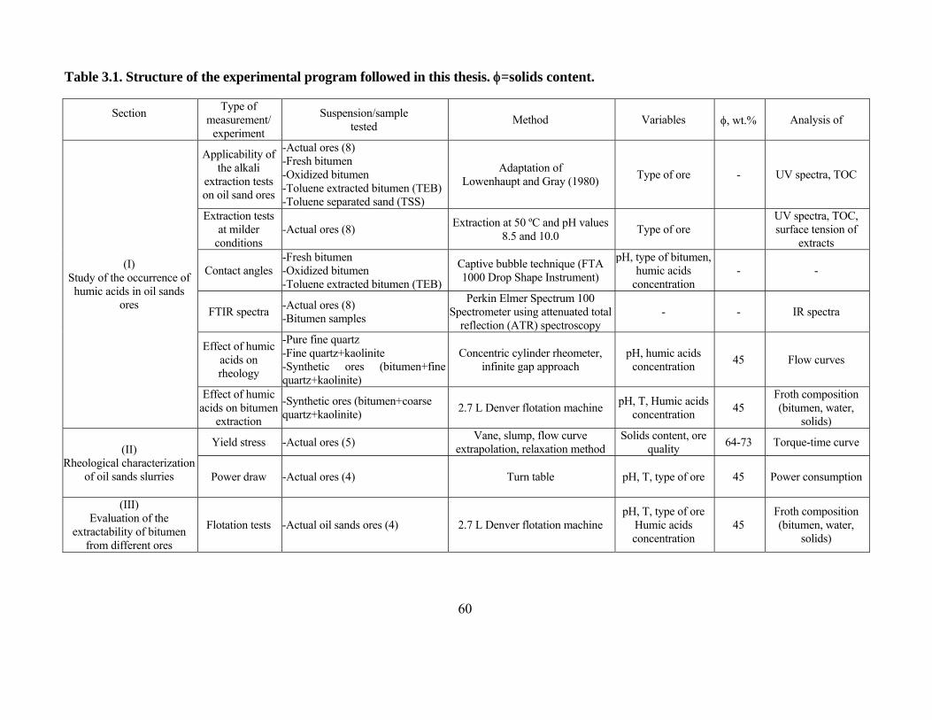
60
Table 3.1. Structure of the experimental program followed in this thesis.=solids content.
Section
Type of measurement/
experiment
Suspension/sample tested
Method Variables , wt.% Analysis of
(I) Study of the occurrence of humic acids in oil sands
ores
Applicability of the alkali
extraction tests on oil sand ores
-Actual ores (8) -Fresh bitumen -Oxidized bitumen -Toluene extracted bitumen (TEB) -Toluene separated sand (TSS)
Adaptation of Lowenhaupt and Gray (1980)
Type of ore - UV spectra, TOC
Extraction tests at milder
conditions -Actual ores (8)
Extraction at 50 ºC and pH values 8.5 and 10.0
Type of ore UV spectra, TOC, surface tension of
extracts
Contact angles -Fresh bitumen -Oxidized bitumen -Toluene extracted bitumen (TEB)
Captive bubble technique (FTA 1000 Drop Shape Instrument)
pH, type of bitumen, humic acids
concentration - -
FTIR spectra -Actual ores (8) -Bitumen samples
Perkin Elmer Spectrum 100 Spectrometer using attenuated total
reflection (ATR) spectroscopy - - IR spectra
Effect of humic acids on rheology
-Pure fine quartz -Fine quartz+kaolinite -Synthetic ores (bitumen+fine quartz+kaolinite)
Concentric cylinder rheometer, infinite gap approach
pH, humic acids concentration
45 Flow curves
Effect of humic acids on bitumen
extraction
-Synthetic ores (bitumen+coarse quartz+kaolinite)
2.7 L Denver flotation machine pH, T, Humic acids
concentration 45
Froth composition (bitumen, water,
solids)
(II) Rheological characterization
of oil sands slurries
Yield stress -Actual ores (5) Vane, slump, flow curve
extrapolation, relaxation method Solids content, ore
quality 64-73 Torque-time curve
Power draw -Actual ores (4) Turn table pH, T, type of ore 45 Power consumption
(III) Evaluation of the
extractability of bitumen from different ores
Flotation tests -Actual oil sands ores (4) 2.7 L Denver flotation machine pH, T, type of ore
Humic acids concentration
45 Froth composition (bitumen, water,
solids)

61
3.1 Samples and reagents
3.1.1 Oil sands ores
Eight oil sands ores of varying quality were supplied by Canadian Natural Resources Ltd.
Table 3.2 shows a characterization of these ores in terms of bitumen, water and solids contents
(Dean-Stark analysis - Bulmer and Starr, 1979). As can be seen from the wide range of bitumen
concentrations covered by these samples (3.6-15.0 wt.%), the quality of these ores was diverse
including good, average, and poor processing ores. It has to be noted that all the oil sands ores
were stored in freezers at approximately -4 °C so that possible alterations of their properties due
to weathering or aging were kept at minimum.
Table 3.2. Composition of the oil sands samples tested.
Bitumen Water Solids
Ore wt.% wt.% wt.%
1 15.0 1.0 84.0
2 10.7 3.6 84.8
3 10.6 3.0 85.7
4 9.2 4.6 86.2
5 9.4 3.9 86.1
6 6.4 4.3 89.3
7 5.9 4.7 88.9
8 3.6 8.2 88.2
Figure 3.1 presents the particle size distributions of the sand fraction of the ores described
in Table 3.2. The particle size distributions were determined using a Malvern Mastersizer 2000, a
laser-based instrument that measures particle sizes in the range 0.02-2,000 m. The BET
(Brunauer Emmett Teller) specific surface areas of the sand fractions were determined from
nitrogen adsorption using a Quantachrome 1MP analyzer. It has to be pointed out that the sand
fractions were separated from bitumen by repeated washing of the bitumen with toluene. In this
case, a representative sample of 50 g (ratio toluene/ore 2:1) was mixed with toluene in 5
consecutive stages, with every mixing stage following by a filtration stage.
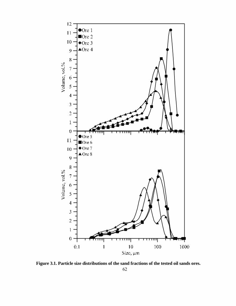
62
Figure 3.1. Particle size distributions of the sand fractions of the tested oil sands ores.
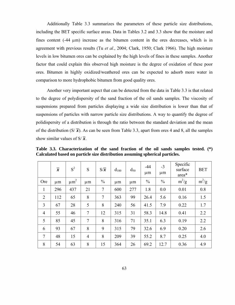
63
Additionally Table 3.3 summarizes the parameters of these particle size distributions,
including the BET specific surface areas. Data in Tables 3.2 and 3.3 show that the moisture and
fines content (-44 m) increase as the bitumen content in the ores decreases, which is in
agreement with previous results (Tu et al., 2004; Clark, 1950; Clark 1966). The high moisture
levels in low bitumen ores can be explained by the high levels of fines in these samples. Another
factor that could explain this observed high moisture is the degree of oxidation of these poor
ores. Bitumen in highly oxidized/weathered ores can be expected to adsorb more water in
comparison to more hydrophobic bitumen from good quality ores.
Another very important aspect that can be detected from the data in Table 3.3 is that related
to the degree of polydispersity of the sand fraction of the oil sands samples. The viscosity of
suspensions prepared from particles displaying a wide size distribution is lower than that of
suspensions of particles with narrow particle size distributions. A way to quantify the degree of
polidispersity of a distribution is through the ratio between the standard deviation and the mean
of the distribution (S/ ). As can be seen from Table 3.3, apart from ores 4 and 8, all the samples
show similar values of S/ .
Table 3.3. Characterization of the sand fraction of the oil sands samples tested. (*) Calculated based on particle size distribution assuming spherical particles.
S2 S S/ d100 d50
-44 m
-3 m
Specific surface area*
BET
Ore m m2 m % m m % % m2/g m2/g
1 296 437 21 7 600 277 1.8 0.0 0.01 0.8
2 112 65 8 7 363 99 26.4 5.6 0.16 1.5
3 67 28 5 8 240 56 41.5 7.9 0.22 1.7
4 55 46 7 12 315 31 58.3 14.8 0.41 2.2
5 85 45 7 8 316 71 35.1 6.3 0.19 2.2
6 93 67 8 9 315 79 32.6 6.9 0.20 2.6
7 48 15 4 8 209 39 55.2 8.7 0.25 4.0
8 54 63 8 15 364 26 69.2 12.7 0.36 4.9

64
Table 3.4 shows the mineralogical composition of the sand fraction of samples 2 to 8. It
can be seen that quartz is the most abundant mineral in the sand, with concentrations above 80
wt.%, and that clay minerals tend to accumulate in the fines fraction. For example, the overall
kaolinite content in ore 8 is 5.7 wt%, and it increases to 9.4 wt% in the fines fraction. This is a
concentration ratio of 1.7. Even more dramatic is the case of ore 2 having almost 5 times more
kaolinite in the fines than in the overall sample. Ore 1 sample was obtained from Alberta
Research Council, and corresponded to a very good processing ore, and was used primarily as a
source of bitumen. Therefore, the sand fraction of ore 1 was expected to contain mainly quartz
with very low amounts of clays.
Table 3.4. Mineralogy of the sand fraction of oil sands samples tested. These results were obtained by XRD.
Quartz Kaolinite Anatase K-feldspar Muscovite
Ore 2 Total sample 91.5 1.8 - 4.6 2.0
-44 m size fraction 73.0 8.8 0.5 8.3 8.8
Ore 3 Total sample 89.0 3.0 - 4.7 3.3
-44 m size fraction 67.3 13.3 0.8 5.9 11.8
Ore 4 Total sample 89.3 4.2 - 3.6 2.9
-44 m size fraction 83.6 6.4 - 5.0 5.0
Ore 5 Total sample 87.4 4.2 0.1 5.1 3.0
-44 m size fraction 65.1 15.9 0.9 6.5 10.8
Ore 6 Total sample 94.1 2.0 - 2.6 1.3
-44 m size fraction 88.1 3.7 - 4.5 3.4
Ore 7 Total sample 81.3 7.5 0.3 5.5 5.3
-44 m size fraction 63.4 17.1 0.9 5.6 12.6
Ore 8 Total sample 85.3 5.7 0.4 4.4 4.3
-44 m size fraction 78.5 9.4 0.6 4.8 5.7

65
3.1.2 Quartz and kaolinite samples
Samples of fine and coarse quartz, and fine kaolinite were also used for tests on such model
materials. As was described in Table 3.1, rheological measurements were performed on slurries
of fine quartz, fine quartz plus kaolinite, and on synthetic oil sands ores (fine
quartz+kaolinite+bitumen) in order to study the effect of humic acids on the rheology of well-
defined model suspensions. Coarse quartz was also used to make synthetic ores that were used to
test the effect of humic acids on flotation. Figure 3.2 shows the particle size distributions of the
samples of fine quartz, coarse quartz, and fine kaolinite.
Fine quartz was obtained from Alfa Aesar Company. The commercial product was 99.5
wt% silicon (IV) oxide, with a measured density of 2.60 g/cm3. The measured mean particle size
for fine quartz was 3.6 m, with 100 vol.% of particles falling below 17.6 m. The measured
specific surface area was 6 m2/g, and x-ray diffraction analysis confirmed that the material was
quartz indeed. The sample of coarse quartz used in this thesis corresponded to a milky variety of
quartz obtained from Ward`s Natural Science Establishment. This sample was dry-ground in a
porcelain ball mill. The data from the supplier indicated that this sample was a nearly pure
chemical compound of silicon and oxygen with density of 2.65 g/cm3. The measured particle size
distribution showed that around 2.9 vol.% of the particles were finer than 44 m. The measured
specific surface area was around 1.2 m2/g. Samples of kaolinite were provided by Ward’s
Natural Science Establishment. These samples were dry-ground in a porcelain ball mill. X-ray
diffraction analysis showed a mineralogical composition of 95.9 wt.% kaolinite, 1.5 wt.% quartz,
1.1 wt.% muscovite and 1.5 wt.% anatase. The measured specific gravity was 2.34 g/cm3. The
measured mean particle size for ground kaolinite was 8.9 m, with 100 vol.% of the particles
being smaller than 55.8 m. The measured specific surface area was 10.9 m2/g.
3.1.3 Reagents
Sodium chloride (NaCl) was used to prepare background solutions while a 1M sodium
hydroxide (NaOH) solution was used to adjust pH. A sodium salt of humic acid obtained from
Aldrich Chemicals was used to prepare humic acids solution of varying concentrations. Vermeer
(1996) reported for this type of humic acids an elemental composition of 55.8 % C, 38.9 % O,
4.6 % H; 0.6 % N, and an average molecular weight of 21,000.

66
Figure 3.2. Particle size distributions of pure samples of fine quartz, coarse quartz, and fine kaolinite.
3.2 Procedures, methods and equipment
Following the structure presented in Table 3.1, a description of the different procedures,
methods and equipment used during the experimental program is given in the following pages.
3.2.1 Alkali-extraction tests
Alkali extraction tests were done on all eight oil sands ores listed in Table 3.2, adapting the
procedure developed by Lowenhaupt and Gray (1980) for coal. The procedure involved mixing a
given amount of ore sample with 100 mL of 1M NaOH solution in a 250 mL beaker. The
amounts of ore samples used in the tests were chosen such that the amount of bitumen in the
samples was always 1 gram. The beaker was placed on a hot plate and heated until boiling. The
Vol
ume,
vol.%

67
suspension was kept under boiling conditions for three minutes, and then the beaker was
removed from the hot plate and allowed to cool down for 0.5 h under a fume hood. The mass of
water that was evaporated during the test was accounted for by weighing the beaker plus slurry
before and after the test. This mass difference was made up with fresh water in order to have the
same volume of solution in all the tests. The resulting mixtures were centrifuged and filtered to
obtain clear solutions containing the alkali-extracted components released from the samples.
These extracts were analyzed in a Cary 50 Scan UV-Visible spectrophotometer using a cell with
a 1-cm optical path length to determine UV-Visible spectra from which the transmission of light
through the alkali extracts was obtained. Then, using the Beer-Lambert law (Equation 3.1) the
absorbance at 520 nm (Abs520) can also be obtained.
3.1
Where I0 and I are the light intensities before and after light passes through the liquid
respectively.
All the solutions were also analyzed for the total organic carbon content (TOC) in a
Shimadzu TOC-VCPH Total Organic Analyzer. TOC measurements required some additional
precautions. All the samples were first diluted to reduce the concentration of residual NaOH, and
afterwards acidified to pH 2 so that the inorganic carbon present in these samples (primarily as
carbonates) was driven off as carbon dioxide before TOC analysis.
Alkali-extraction tests were also performed on samples of pure and artificially oxidized
bitumen extracted from ore 1. Bitumen oxidation was achieved by placing a sample of fresh
bitumen in an oven for 7 days at 60 ºC with air circulation.
Samples of bitumen extracted from the tested ores were also analyzed using the alkali
extraction method. The procedure consisted of mixing a given amount of ore with toluene at a
volume ratio of 1:2. The resulting mixture of bitumen, sand, and toluene was filtered using a
filter paper so that the sand fraction was separated first. Then, toluene was allowed to evaporate
and the remaining sample of bitumen was used for the alkali extraction tests. The so-obtained

68
samples of sand separated from bitumen of the different types of ores were also tested using the
alkali extraction tests in order to study the distribution of humic acids between solids and
bitumen.
3.2.2 Extraction tests at milder conditions
Additional leaching experiments were performed on the tested oil sands ores, but in this
case under much milder conditions than those used in alkali-extraction tests. The idea was to use
conditions similar to those of the actual bitumen extraction process to determine the extent of
leaching of organic matter from the ores. pH values in these experiments varied between 8.5, and
pH 10, and temperature was kept at 50 °C. The procedure consisted of mixing an appropriate
amount of ore (containing 1 g of bitumen) with 100 mL of 0.01 M NaCl solution conditioned at
50 ºC and at desired pH in a 250 mL beaker. The beaker was placed on a hot plate, and heated in
order to maintain 50 ºC for a period of 6 minutes. After this, the beaker was removed from the
hot plate, and allowed to cool for 0.5 h. The resulting suspensions were centrifuged and filtered
to obtain clear solutions. Samples of the resulting solutions were analyzed in a Cary 50 Scan UV-
Visible spectrophotometer as in alkali-extraction tests, and also analyzed for the total organic
carbon content (TOC) in a Shimadzu TOC-VCPH Total Organic Carbon Analyzer.
In order to assess the surface activity of the leached organic compounds, surface tension
measurements were performed on these solutions using the Lecomte Du Noüy ring method
(Lecomte Du Noüy, 1919) with a CENCO-Du Noüy tensiometer. In this method the surface
tension is obtained from the determination of the mechanical force required to pull up a platinum
ring of known ring radius (RR) from the solution surface. The relationship between the force, the
ring radius, and the surface tension can be described by Equation 3.2 (Masutani and Stenstrom,
1984).
4 3.2
Where γLV is the surface tension between liquid and vapor, F is the force necessary to
detach the ring from the liquid, and f is the Harkins-Jordan correction factor that depends on the

69
dimensions of the ring and on the volume of liquid displaced by pulling the ring. In all the
experiments the metal ring was kept clean by washing with distilled water, and flamed before
every experiment.
3.2.3 Contact angle measurements
Contact angle measurements were performed on bitumen samples using the captive bubble
technique in a FTA 1000 Drop Shape Instrument. Figure 3.3 (a) shows a schematic of the
methodology used to measure the contact angles. The procedure started by attaching an air
bubble with a volume of 5 L to a layer of bitumen coated on a glass slide. Coating of glass
slides with bitumen was carried out using a SCS 6800 spin coater rotating at 2,000 rpm. In order
to produce a smooth coating, pure bitumen was first heated up to reduce its viscosity, and then
spread on the glass slide which was then rotated at high speeds in the spin coater. After attaching
the small bubble to bitumen, images of the variation of the bubble shape were obtained at times
determined by a time multiplier of 1.04, and for a total period of 7 minutes. Then the contact
angles were analyzed using the FTA software. The baseline along the contact line between the air
bubble and bitumen, and the curvature of the air bubble are first defined as shown in Figure 3.3
(b). Then, the software computes the contact angle as the angle between the tangent to the bubble
curvature at the contact point with the baseline and the baseline itself. Figures 3.3 (c) and (d)
show examples of contact angles for strongly hydrophobic bitumen as well as for a slightly
hydrophobic bitumen. The liquid phase in these experiments was a solution of 0.01M NaCl, and
tests were done at different pH values (3, natural, and 10.5), and at room temperature (~20 ºC).
The effect of humic acids on the wettability of bitumen was also assessed through contact angles
measurements.
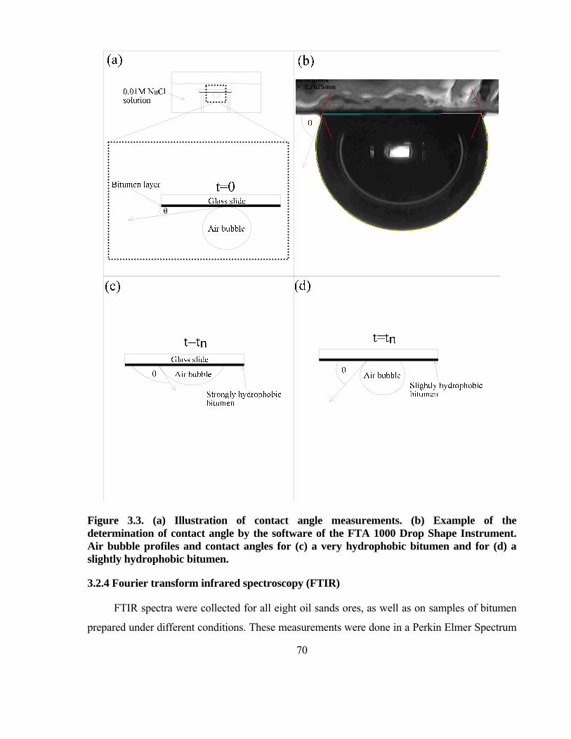
70
Figure 3.3. (a) Illustration of contact angle measurements. (b) Example of the determination of contact angle by the software of the FTA 1000 Drop Shape Instrument. Air bubble profiles and contact angles for (c) a very hydrophobic bitumen and for (d) a slightly hydrophobic bitumen.
3.2.4 Fourier transform infrared spectroscopy (FTIR)
FTIR spectra were collected for all eight oil sands ores, as well as on samples of bitumen
prepared under different conditions. These measurements were done in a Perkin Elmer Spectrum

71
100 FTIR (Fourier Transform Infrared) Spectrometer using a diamond-coated KRS5 crystal. This
instrument uses the principles of Attenuated Total Reflection (ATR) spectroscopy. In this
technique, an infrared beam is directed onto a crystal of high refractive index as shown in Figure
3.4. Typical crystals have refractive indexes between 2.38 and 4.01 at 2,000 cm-1. Due to the
differences between the refractive indices of the studied sample and the crystal, an internal
reflectance is obtained which creates an evanescent wave that prolongs beyond the surface of the
crystal into the sample that is in close contact with the crystal. The evanescent wave extends
beyond the crystal surface by about 0.5-5 microns. The evanescent wave is attenuated by the
interactions with the studied sample, and the resulting attenuated IR beam exits at the opposite
end of the crystal and is sensed by the IR detector generating an infrared spectrum. FTIR
measurements in this work were done by collecting continuous scans in the wavenumber range
from 600 to 4,000 cm-1 at a resolution of 0.5 cm-1.
Figure 3.4. Schematic of attenuated total reflection spectroscopy (ATR).
3.2.5 Effect of humic acids on rheology
Rheological measurements were done in order to study the effect of humic acids on the
rheology of slurries of fine quartz, mixtures of fine quartz (95 wt.%) and kaolinite (5 wt.%), and
mixtures of fine quartz (95 wt.%) with kaolinite (5 wt.%) whose particles were coated with
bitumen to give a 10 wt.% bitumen content (with respect to the total mass of bitumen+fine
quartz+kaolinite). This bitumen was extracted from ore 1 by applying three flotation stages at 50
°C (1 rougher and 2 cleaner with distilled water) without using any reagents. The viscosity of so

72
recovered bitumen at 50 ºC was around 2 Pas (Gutierrez, 2009). In order to achieve a good
coating of bitumen onto the solid particles, bitumen was first dissolved in toluene at a ratio of 3
mL toluene per 1 g bitumen. The organic solution of bitumen was mixed with particles of pure
solids (fine quartz and kaolinite), and homogenized in order to spread the bitumen solution over
all the mineral particles. Then, the mixture was kept under a fume hood for 1 week to completely
evaporate toluene. In order to avoid the formation of lumps, and to produce a homogeneous feed
for the experiments, the synthetic ore samples were screened using a 4.76 mm sieve.
Before rheological measurements, all the slurries were prepared at 45 wt.% solids using a
solution 0.01M NaCl with and without Aldrich humic acids. The mixing volume was 800 mL,
and the slurries were mixed for 25 minutes using an IKA RW20 mixer set at an impeller speed of
500 rpm. The stirring speed was chosen arbitrarily while the mixing time of 25 minutes was
found to produce a constant pH value. The pH was adjusted using a 1M NaOH.
In the case of slurries of fine quartz, and mixtures of fine quartz (95 wt.%) and kaolinite (5
wt.%), the rheological measurements were conducted using a Haake VT550 viscometer
connected to a MV1-P fixture, single gap, bob-in-cup geometry, with an inner cup diameter of
40.08 mm and a gap of 0.96 mm. The surfaces of this fixture were grooved so that wall slip can
be kept at minimum. Standard rheological flow curves were obtained by increasing the shear rate
between 0 and 600 s-1 in 90 s, and decreasing the shear rate from 600 to 0 s-1 in 90 s. All these
experiments were performed at room temperature (~21 ºC), and at pH values of 3.0, and 8.5.
In the case of slurries of mixtures of bitumen, fine quartz and kaolinite, rheological
measurements were done at room temperature (~21 ºC), and at pH 3.0, 8.5, and 10.0. The
rheological flow curves at pH 3.0, and 8.5 were determined using the infinite gap approach
previously described in section 2.7.4.3. The rotating surface in these experiments was a vane of
0.5 cm diameter and 6 cm height. These dimensions were chosen in order to follow the
recommendations made by Fisher et al. (2007) to reduce the end effects. A Haake Rotovisco
VT550 rotational viscometer was used with vane at different rotational speeds. Then, changes in
torque with time were recorded for a period of 120 s, and the equilibrium torque was determined
and used to calculate the shear stresses. At the same time the shear rates were calculated using
the procedure explained in Section 2.7.4.3 for the infinite gap approach. At pH 10 the slurry
viscosities were much lower than at pH values 3, and 8.5. In this case the torque readings
73
obtained from the rotation of the vane of 0.5 cm diameter and 6 cm height were very low, close
to the lower limit of the Haake Rotovisco VT550, and it was not possible to use the infinite gap
approach to obtain the flow curves. In this case, the rheological flow curves were obtained using
the same MV1-P fixture used for slurries of fine quartz, and quartz and kaolinite.
3.2.6 Effect of humic acids on bitumen extraction
The effect of humic acids on bitumen extraction was assessed through flotation
experiments performed on samples of artificial mixtures of bitumen and a solid portion
containing coarse quartz (95 wt.%) and kaolinite (5 wt.%). These solids were coated with
bitumen using the same procedure explained in the previous section. The bitumen content in this
mixture was 10 wt.% (out the total mass of bitumen+coarse quartz+kaolinite). The experiments
were done in a standard Denver flotation machine using a 2.7 L flotation cell. Slurries were
prepared at 45 wt.% solids using solutions of 0.01 M NaCl, and the flotation tests were done at
pH 8.5, and 10, and at 50 ºC, in the presence and absence of Aldrich humic acids. Froth was
collected at times of 0.5, 1, and 4 minutes. The pulp level in the flotation cell was kept constant
by adding background solution with the same composition, pH and temperature as those of the
test.
3.2.7 Yield stress measurements
Yield stress measurements were performed on concentrated slurries prepared with five
different oil sands ores (2, 3, 5, 6, and 7), at solids contents varying between 64 and 73 wt.%.
Samples 1, 4, and 8 were not tested because of the insufficient amount of these samples. Slurries
for these tests were prepared using ores samples that were previously sieved through a 5.0 mm
screen in order to avoid the presence of lumps and to produce homogeneous suspensions. A
solution of 0.01M NaCl was used in these experiments as the background electrolyte, and slurries
were made by manually mixing the ore samples with the aqueous solution for 3 minutes, which
was followed by a resting time of 0.5 minutes before performing the tests. Some precautions
were taken in order to remove as much air as possible which was done by gently stirring the
slurries with a glass rod. All the yield stress measurements were carried out at room temperature
(21 ºC).
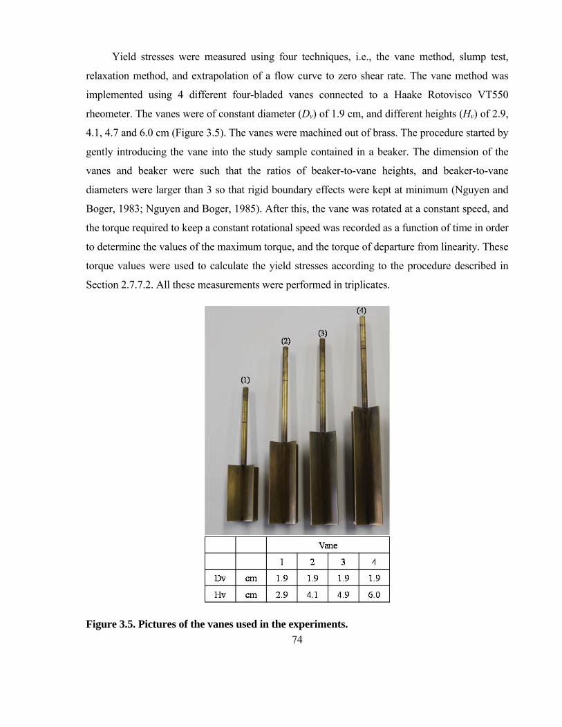
74
Yield stresses were measured using four techniques, i.e., the vane method, slump test,
relaxation method, and extrapolation of a flow curve to zero shear rate. The vane method was
implemented using 4 different four-bladed vanes connected to a Haake Rotovisco VT550
rheometer. The vanes were of constant diameter (Dv) of 1.9 cm, and different heights (Hv) of 2.9,
4.1, 4.7 and 6.0 cm (Figure 3.5). The vanes were machined out of brass. The procedure started by
gently introducing the vane into the study sample contained in a beaker. The dimension of the
vanes and beaker were such that the ratios of beaker-to-vane heights, and beaker-to-vane
diameters were larger than 3 so that rigid boundary effects were kept at minimum (Nguyen and
Boger, 1983; Nguyen and Boger, 1985). After this, the vane was rotated at a constant speed, and
the torque required to keep a constant rotational speed was recorded as a function of time in order
to determine the values of the maximum torque, and the torque of departure from linearity. These
torque values were used to calculate the yield stresses according to the procedure described in
Section 2.7.7.2. All these measurements were performed in triplicates.
Figure 3.5. Pictures of the vanes used in the experiments.
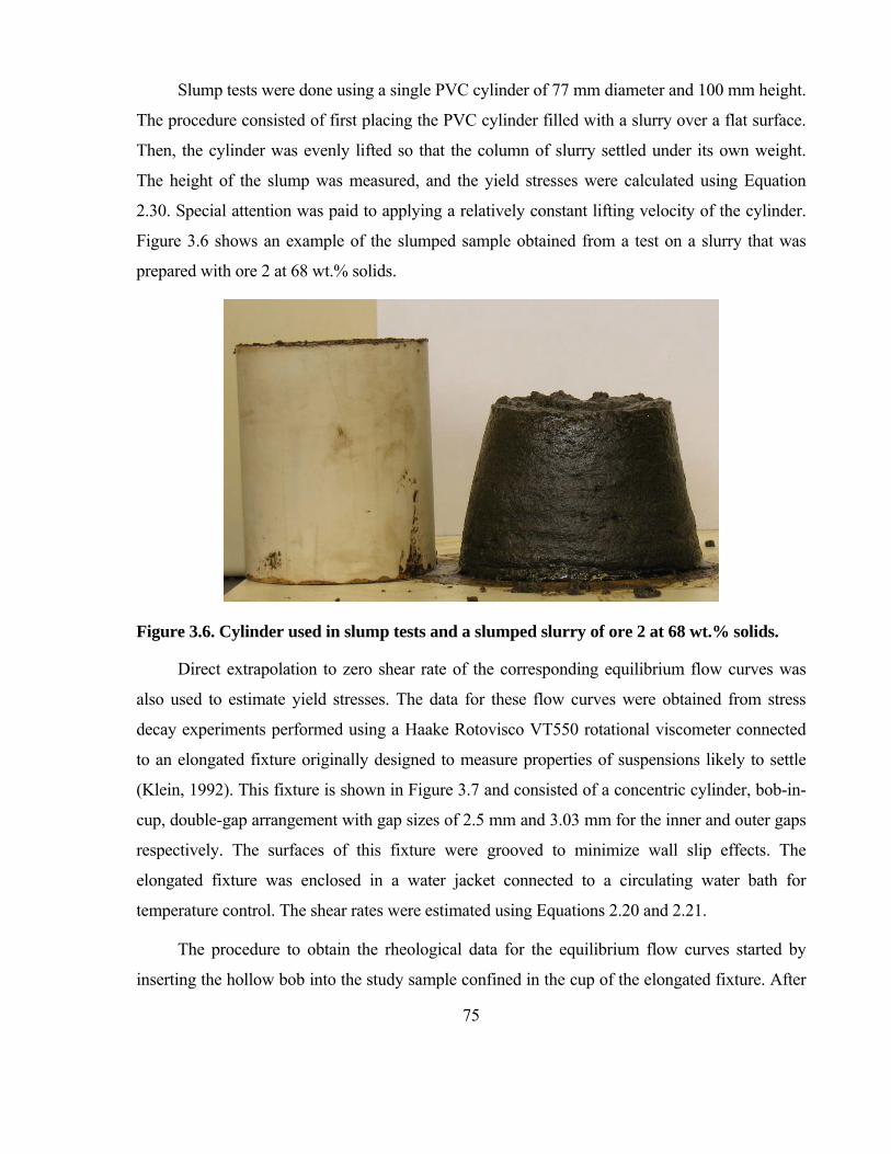
75
Slump tests were done using a single PVC cylinder of 77 mm diameter and 100 mm height.
The procedure consisted of first placing the PVC cylinder filled with a slurry over a flat surface.
Then, the cylinder was evenly lifted so that the column of slurry settled under its own weight.
The height of the slump was measured, and the yield stresses were calculated using Equation
2.30. Special attention was paid to applying a relatively constant lifting velocity of the cylinder.
Figure 3.6 shows an example of the slumped sample obtained from a test on a slurry that was
prepared with ore 2 at 68 wt.% solids.
Figure 3.6. Cylinder used in slump tests and a slumped slurry of ore 2 at 68 wt.% solids.
Direct extrapolation to zero shear rate of the corresponding equilibrium flow curves was
also used to estimate yield stresses. The data for these flow curves were obtained from stress
decay experiments performed using a Haake Rotovisco VT550 rotational viscometer connected
to an elongated fixture originally designed to measure properties of suspensions likely to settle
(Klein, 1992). This fixture is shown in Figure 3.7 and consisted of a concentric cylinder, bob-in-
cup, double-gap arrangement with gap sizes of 2.5 mm and 3.03 mm for the inner and outer gaps
respectively. The surfaces of this fixture were grooved to minimize wall slip effects. The
elongated fixture was enclosed in a water jacket connected to a circulating water bath for
temperature control. The shear rates were estimated using Equations 2.20 and 2.21.
The procedure to obtain the rheological data for the equilibrium flow curves started by
inserting the hollow bob into the study sample confined in the cup of the elongated fixture. After

76
this, a resting time of 1 minute was given before the rheometer was started. The shear rate was
increased from 0 to 20 s-1 over a period of 120 seconds. The shear rate was kept constant at that
value for 90 seconds, after which it was suddenly changed from 20 s-1 to a different target value.
The samples were sheared at these final values for a period of 200 seconds so that equilibrium
shear stresses could be reached. Since the bob of the fixture is essentially a hollow cylinder,
inserting such a bob into the sample minimized the distortion of the slurry network. This aspect is
important when testing thixotropic samples and, as the results by Gutierrez and Pawlik (2012)
showed, oil sands slurries are likely to display a strongly thixotropic response.
Figure 3.7. Representation of the elongated fixture used in rheological measurements and the Haake Rotovisco VT550. r1= 16.5 mm, r2= 19.0 mm, r3= 20.0 mm, r4= 23.03 mm.
The yield stresses of concentrated oil sands slurries were also estimated using the
relaxation method. The same elongated fixture illustrated in Figure 3.7 was used in these
experiments. The procedure followed in these measurements consisted of pre-shearing oil sand
slurries at a given shear rate for a period of 180 seconds. After this, the shear rate was suddenly
lowered to zero, and the shear stresses were recorded as a function of time during another 180
seconds. Pre-shearing was carried out at shear rates of 10, 20, 30, and 40 s-1.

77
3.2.8 Power draw measurements
The process of gravity separation or flotation of bitumen in oil sands processing is in
general carried out at more diluted solids concentrations (around 30 to 45 wt.%) than those of the
conditioning stage. The residence time in the hydrotransport pipeline is around 25 min.
Therefore, reliable rheological measurements on these types of diluted slurries over a period of
25 minutes are very difficult due to particle settling. It was mainly because of the timescale of the
test, that it was decided to use power draw measurements to follow changes in viscosity of these
slurries over such extended periods of time.
Power draw measurements were based on the torque method using a turn-table setup
schematically shown in Figure 3.8. The turn-table arrangement consisted of a conditioning vessel
(flotation cell) that was placed on a low friction disc that rotated as a result of the torque exerted
on the slurry by the impeller. A lever arm was attached horizontally to the base of the low
friction disc. This arm was connected through a thin wire to a force gauge that was capable of
taking readings every 2 seconds. Since the force imparted onto the fluid by the impeller caused
an equal and opposite force on the lever arm, the gauge reading could be directly related to the
force applied to the pulp, and this force could be correlated to the power consumption per unit
volume of slurry according to Equation 3.3.
P =F×9.807x10 ×L×rpm×2π×1.6667x10
V 3.3
Where, Pv is the power input in Watts per cubic meter, L is the lever arm length in m, rpm
is the shaft speed in rotations per minute, F is the gram-force readout obtained from the force
gauge, and Vs is the slurry volume in m3. The factor 9.807x10⁻³ corresponds to the gravitational
acceleration divided 1000 and is used in Equation 3.3 to convert the force in grams-force to
Newton, while the factor 2π×1.6667x10 converts rpm into rad/s. The mixing container used
in these measurements was a 2.7 L Denver flotation cell that contained 2.1 L of slurry. The lever
arm length was 9 cm long, and the slurries were stirred at 800 rpm. A LIGHTNIN LabMasterTM
mixer was used as a stirrer, which kept the mixing speed at a constant value regardless of the

78
slurry viscosities. The control of temperature was achieved using heating straps wrapped around
the outside walls of the cell. It was found that the heating straps did not significantly contribute to
the total torque read-outs. It should be recognized that this turn-table design was previously used
by Genc (2009) for measuring the power consumption of nickel sulfide slurries with good results.
The concept of power draw measurements to evaluate the aggregation of mineral particles under
flotation conditions was also used by Lapidot and Mellgren (1968).
Slurries of four types of ores were tested through power draw measurements, i.e., ores 2, 3,
5, and 7, under different conditions of pH (8.5, 10), and temperature (20, 50 ºC). pH was adjusted
using a 1 M NaOH solution, and slurries were prepared using a 0.01 M NaCl solution. No
aeration was applied in these tests, and the slurries were mixed for 25 minutes. For tests at 50 ºC,
slurries were prepared by preheating a background solution in a stainless steel beaker to a
temperature higher than desired which, after the oil sand sample was mixed with this background
solution, produced slurries at a target temperature.
3.2.9 Evaluation of the extractability of bitumen from different ores
Bitumen extraction was assessed using bench scale flotation experiments in a standard
Denver flotation machine using a 2.7 L flotation cell. Four types of ores were tested through
flotation tests, i.e., ores 2, 3, 5, and 7, under different conditions of pH (8.5, 10), and temperature
(20, 50 ºC). pH was adjusted using a 1 M NaOH solution, and slurry volumes of 2.1 L were
prepared using a 0.01 M NaCl solution. The control of temperature was achieved using heating
straps in the same way as for the turn-table set-up. The power draw measurements described in
the previous section simultaneously served as a feed conditioning and preparation stage for
flotation tests. Therefore, it was possible to directly correlate power draw required for
conditioning with subsequent bitumen extraction. The conditioned slurries obtained from the
turn-table were afterwards re-conditioned in the Denver flotation machine for 2 minutes at 1,200
rpm. After this, the air valve was opened, and the bitumen froth was collected under continuous
aeration at 0.5, 1, 4, and 8 minutes of the flotation process. The pulp level in the flotation cell
was again kept constant by adding the background solution conditioned at the pH and
temperature of the test. Bitumen, solids and water content in the froth streams were analyzed
using the standard Dean-Stark method (Bulmer and Starr, 1979).

79
Figure 3.8. Schematic of the turn-table setup.
80
4 Results and discussion
4.1 Study of the occurrence of humic acids in oil sands ores
The main objective of this section is to develop a methodology to quantify the levels of
humic acids in oil sands ores so that their effects on rheology, power draw, and bitumen
extraction can more clearly be assessed.
4.1.1 Applicability of the alkali extraction tests to oil sand ores
As was explained in the literature review, Lowenhaupt and Gray (1980) developed the
alkali extraction test to quickly determine the oxidation of bituminous metallurgical coals. The
test for coal involves boiling a small sample of ground coal in a concentrated sodium hydroxide
solution and measuring the absorbance of that solution at a wavelength of 520 nm using a
spectrophotometer. The alkali extraction test relies on the fact that oxidation of bituminous coal
leads to a gradual enrichment of the coal surfaces in humic matter containing various types of
oxygen functional groups, most of which are of acidic nature (carboxylic, phenolic, etc.). When
exposed to strongly alkaline solutions, these products of oxidation dissolve in solution giving it a
characteristic yellow-brown color. The intensity of this color is a measure of the amount of
humic acids on the coal surface and therefore also of the extent of coal oxidation.
In this section, the test will be applied to oil sand ores with the main objective to quantify
the occurrence of humic acids within the tested ores. Figure 4.1 illustrates images of the alkali
extracts obtained from the tested ores. It can clearly be observed that the yellow-brown color
(tea-like appearance), which is associated with the presence of humic substances in solution,
becomes darker as the quality of the ores decreases from ore 1 to ore 8. This result reveals that
poor ores characterized by a low content of bitumen and a high content of fines also exhibit the
highest tendency to leach large amounts of humic acids under the alkali extraction conditions.

81
Figure 4.1. Images of the alkali extracts obtained from alkali extraction tests on ores 1 through 8.
Figure 4.2 (a) illustrates the UV-Visible spectra of the same alkali extracts shown in Figure
4.1. The data show that the spectra move towards higher values of absorbance (low
transmittance) as the processability of the ores decreases indicating a correlation between the
results from the alkali extraction tests and the quality of the ores. The corresponding total organic
carbon (TOC) contents in the alkali extracts are given in Figure 4.2 (b). As can be seen, the TOC
values range from 63 mg/L for extracts of ore 1 to 174 mg/L and 263 mg/L for ores 7 and 8,
respectively.
As was explained previously, all these alkali extraction tests were standardized in such a
way that each ore sample contained 1 g of bitumen. As bitumen contents in the samples were
different, the masses of these samples required to contain 1 g of bitumen for the tests were also
different. For example, the masses of ores 1 (15 wt.%) and 8 (3.6 wt.% bitumen) that contain 1 g
of bitumen are 6.7 g (1/0.15) and 27.8 g (1/0.036), respectively. Therefore, the TOC data should

82
be viewed as relative amounts of organic matter per gram of bitumen. In other words, 1 gram of
bitumen from ore 1 is associated with a 4 times lower amount of alkali-soluble organic matter
than 1 gram of bitumen from ore 8. The same is valid for the absorbance values, so the amounts
of humic acids in the extracts obtained from different ores should also be viewed as relative per
gram of bitumen. It is, however, very difficult to conclude at this point whether the leached
organic matter, presumably humic acids, originated entirely from bitumen or whether they were
naturally present in the ore as a separate chemical compound.
Figure 4.3 (a) shows a plot of the TOC values in the alkali extracts as a function of
absorbance at a wavelength of 520 nm (Abs520). It can be seen that there is a direct correlation
between these two variables suggesting that the organic carbon concentration in the extracts is
proportional to the amount of alkali-extracted organics. Attempts were also made to correlate the
values of Abs520 with various characteristics of the ores, such as the bitumen and fines contents,
moisture content, average particle size, etc. It was found that the best correlation was obtained
when the Abs520 parameter was plotted as a function of the dimensionless ratio of the fines
content (-44 m size fraction) to the bitumen content as shown in Figure 4.3 (b). This is a very
interesting result since the industrial practice shows that bitumen recovery increases with
bitumen content and decreases with the fines content (Masliyah et al., 2004).
It is also possible to present the alkali extraction data as the equivalent weight percent
content of Aldrich humic acids in the ore samples, and as the mass of humic acids (grams) per
mass of bitumen (tonne). These results are shown in Figure 4.4. The equivalent Aldrich humic
acids concentrations were determined using a calibration curve (Abs520 vs Aldrich humic acid
concentration) presented in Appendix A. It can be seen that when the amounts of humic acids are
expressed as the percentage of ore mass (Figure 4.4 (a)), only ore 1 stands out as containing the
lowest quantity of humic acids, and the correlation with the quality/processability of the ores is
not very clear. However, a better trend with ore quality can be seen when the amount of humic
acids is expressed per mass of bitumen.

83
Figure 4.2. (a) UV-Visible spectra and (b) total organic carbon of extracts obtained from alkali-extraction tests on the ore samples.

84
Figure 4.3. (a) Correlation between TOC and Absorbance at 520 nm (Abs520) of solutions obtained from alkali-extraction tests on the 8 oil sands samples. (b) Correlation between Absorbance at 520 nm (Abs520) and the ratio of the fines content (-44 m size fraction) to bitumen content.
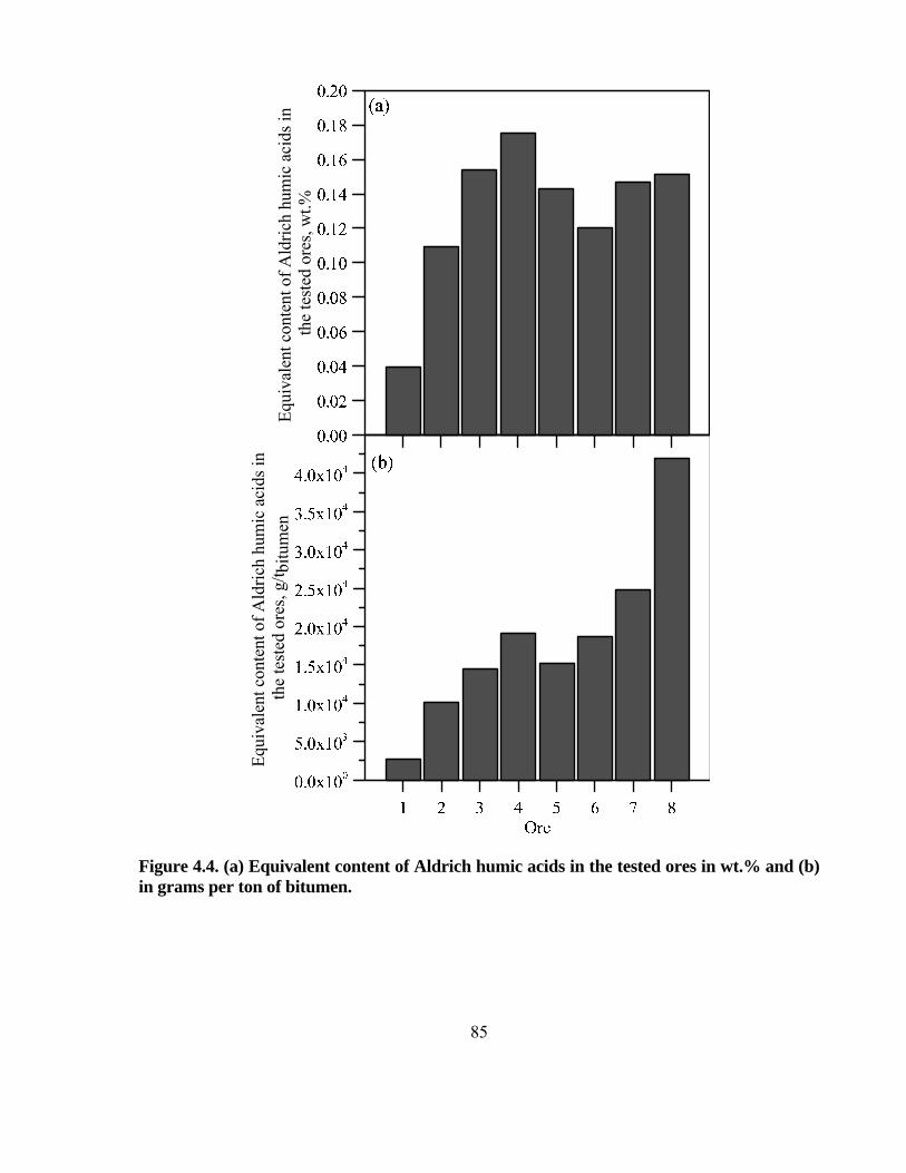
85
Figure 4.4. (a) Equivalent content of Aldrich humic acids in the tested ores in wt.% and (b) in grams per ton of bitumen.
Equ
ival
entc
onte
ntof
Ald
rich
hum
icac
ids
inth
ete
sted
ores
,g/t b
itum
enE
quiv
alen
tcon
tent
ofA
ldri
chhu
mic
acid
sin
the
test
edor
es,w
t.%

86
A comparison between the UV/Visible spectra of solutions obtained from the alkali-
extraction tests and spectra of solutions of Aldrich humic acids is shown in Figure 4.5. It has to
be noted that the corresponding solutions of Aldrich humic acids were prepared at the same TOC
values as the solutions obtained from the alkali-extraction tests. If the TOC of the extracts
originated entirely from humic acids, then the two spectra should ideally overlap, or at least be
very close together, although it is difficult to expect that humic acids from Aldrich would show
the same chemical composition, and hence the same spectra, as humic acids leached from the
ores. Nevertheless, the data in Figure 4.5 show that at the same TOC level (63 mg/L) the
spectrum for the alkali-extract of ore 1 and the spectrum for a solution prepared from commercial
humic acids are quite different. This result strongly indicates that the TOC content of the extracts
of ore 1 originates from chemical compounds other than humic acids. UV-Visible spectra of
alkali-extracted solutions of ores 2 to 6 resemble much more closely the spectra of Aldrich humic
acids. In the case of ores 7 and 8, which are the poorest types in terms of their quality and
processability, the similarity of the spectra of the alkali extracts and of the commercial humic
acids is the highest. All these results indicate that poor oil sands ores release substantial amounts
of organic matter that shows strong similarities to humic acids. In contrast, good ores do not
release as much of the organic matter, and UV spectra of these leached substances are quite
different from those of typical humic acids. It appears that these good quality ores primarily
release ionic surfactants rather than polyeletrolytes produced as a result of weathering/oxidation.
These results are consistent with previously reported findings about the effect of surfactants on
bitumen extraction. Sanford and Seyer (1979) and Basu et al. (1996) proposed a direct
correlation between liberation/extraction and presence of free surfactants in solution. Moreover,
Schramm et al. (1984b) demonstrated that there is a single equilibrium concentration of
carboxylate surfactants (~1.2 x 10⁻⁴ N) that leads to maximum bitumen recoveries. The same
author explained that the free natural surfactants in solution increase the negative charges at the
oil-solution and solid-solution interfaces, with the oil/solution interface displaying maximum
electrophoretic mobility at the point of maximum efficiency of the hot-water extraction process
(Schramm and Smith, 1985).

87
Figure 4.5. Comparison between the UV/Visible spectra of solutions obtained from alkali-extraction tests and spectra of solutions of Aldrich Humic Acids. Solutions of Aldrich HA were prepared at the same TOC values as those of the alkali-extracted solutions.
Abs
orba
nce
Abs
orba
nce
Abs
orba
nce
Abs
orba
nce

88
4.1.2 Extractions of humic acids at pH values of 8.5 and 10
Experiments were also done in order to study the extractability of humic acids from the oil
sands ores at conditions of temperature and pH similar to those observed in the industrial
extraction process, i.e., 50 °C, and pH 8.5-10.0. Figure 4.6 shows the Abs520 of solutions
obtained from these experiments. It has to be noted that the masses of the samples were again
chosen to contain 1 g of bitumen from each ore. A comparison between the values of Abs520
obtained from these experiments and those from the alkali-extraction tests indicates that leaching
of organic matter is almost insignificant under these experimental conditions. For example,
Abs520 of alkali extracts from ore 8 was around 1.1, but at pH 10.0 and 50 °C this value is only
0.02. It seems that leaching of organics under such relatively mild conditions is not as sensitive to
changes in the quality of the ores as is the drastic alkali extraction test.
Figure 4.6. Abs520 of solutions obtained after contacting a given amount of each ore containing 1 g of bitumen with 0.01 M NaCl solutions at pH 8.5 and 10.0, and at 50 °C.

89
Another important conclusion that can be drawn from Figure 4.6 is that humic acids in the
tested ores are strongly bonded either with bitumen or with the solids, and that they do not occur
as free, easily leachable chemical compounds. It has to be recognized that humic acids are readily
soluble in water under neutral and alkaline conditions, so a small amount of free humic acids in
an ore would easily dissolve in water at pH 8.5 or 10.0, and the corresponding absorbance at 520
nm would be high. However, none of the ores under mild leaching conditions produced
absorbance values comparable with those obtained in the alkali extraction test.
Figure 4.7 shows the results of surface tension and TOC measurements performed on the
solutions obtained from these extraction tests. These results indicate that the organic matter
released from the ores under mild pH and temperature conditions is quite surface active. Even for
poor ores 7 and 8, the Abs520 of these solutions is very low while the TOC is quite high. Since
the surface activity of humic acids can be expected to be very low (Pawlik and Laskowski,
2003), it seems that surfactants rather than humic acids are released into solution under those
mild conditions.
4.1.3 Association of humic acids with ore components
As was explained in the literature review the presence of insoluble organic matter (IOM),
which mainly consists of humic acids (Kotlyar et al., 1988), was reported by several authors
(Charrie-Duhaut et al., 2000; Majid et al., 2000a; Majid et al., 2000b; Majid and Sparks, 1996;
Kotlyar et al., 1988; Kessick, 1979; Majid and Ripmeester, 1990; Majid et al., 1991; Majid et al.,
1992; Ignasiak et al., 1985; Kotlyar et al., 1990; Kotlyar et al., 1985). Based on the alkali
extraction and spectrophotometric results from the previous sections, it is possible to conclude
that a significant proportion of the organic components that are leached from the oil sands ores
under alkali extraction conditions are humic acids. As such, they can be expected to be insoluble
in toluene.
As was discussed earlier, humic acids do not seem to occur as free chemical compounds in
the ores, but are strongly bonded with the ore components. However, it is not entirely clear
whether humic acids are associated with bitumen or with the solids, and the objective of this
section is to investigate how humic acids are partitioned between the solids and bitumen.

90
Figure 4.7. Surface tension and its correlation with the TOC values of solutions obtained at 50 °C and pH values of 8.5 and 10.
91
In order to obtain separate samples of solids and bitumen, ore samples containing 1 g of
bitumen were mixed with 100 mL of toluene, and the resulting mixtures were afterward filtered
through a Whatman filter paper number 2 to obtain a toluene-separated sand (TSS), and a
solution of bitumen in toluene. Toluene was then allowed to evaporate in order to obtain samples
of toluene-extracted bitumen (TEB) and TSS. Then, alkali extraction tests were separately
performed on samples of TSS and TEB, and the alkali extracts were analyzed for TOC and
Abs520. Finally, these two parameters were compared with those obtained from alkali extraction
tests on the original ore samples presented in Figure 4.1.
Table 4.1 summarizes the TOC and Abs520 values of the alkali extracts from raw ores,
TSS, and TEB. By mass balance, the sum of the TOC and Abs520 values obtained from TSS and
TEB should be equal to the values obtained from the alkali extraction test on the raw ore. Except
perhaps ore 4, the agreement between the direct assay and the mass balance calculation
(TSS+TEB) is very good for all ores. It is thus possible to determine the percent contributions of
TSS and TEB to the total TOC and Abs520 of the ores. Looking at the Abs520 data, it can be
seen that the values of Abs520 in the sand fraction are very close to those obtained from the
initial ores samples, while the Abs520 values in the TEB are almost zero. Therefore, it can be
concluded from these results that all the humic acids present in the initial ores samples remained
in the sand fraction after dissolving bitumen away from the solids.
It can be seen that the percentage of TOC in the TSS varies between 55 and 84 % of the
total. At the same time, the Abs520 originates entirely from organics leached from the solids, and
these organics are most likely humic acids since they are insoluble in toluene, and so they stay
with the solids after mixing with toluene. The rest of TOC still remains in TEB which
simultaneously contains no material that contributes to the total Abs520. It is noteworthy that
TEB still released a substantial amount of organic matter during the alkali extraction tests. Since
the Abs520 of TEB was close to zero, it is very likely that the organic compounds released by
TEB were surfactants rather than humic acids. The fact that there is a fraction of the total TOC
(TSS+TEB) that cannot be attributed to the presence of humic acids agrees with the data
presented in Figure 4.5 that showed that for the same total TOC, the UV-Visible spectra of the
alkali extracts and of humic acids solutions did not overlap, particularly for good ores.

92
Table 4.1. Results obtained from alkali extraction tests on samples of toluene-separated sand (TSS) and toluene-extracted bitumen (TEB).
TOC in extracts from alkali extraction tests on samples of ores, TSS, and TEB Ore TSS TEB TSS+TEB mg/L mg/L % of TSS+TEB mg/L % of TSS+TEB mg/L Ore 1 63 36 55 29 45 65 Ore 2 102 81 76 25 24 105 Ore 3 126 85 64 48 36 133 Ore 4 158 119 84 23 16 142 Ore 5 146 114 77 35 23 150 Ore 6 157 121 73 45 27 166 Ore 7 174 122 75 40 25 162 Ore 8 263 208 83 44 17 253 Abs520 of extracts from alkali extraction tests on samples of ores, TSS, and TEB Ore TSS TEB TSS+TEB
% of TSS+TEB % of TSS+TEB Ore 1 0.02 0.04 100 0.00 0 0.04 Ore 2 0.23 0.24 96 0.01 4 0.25 Ore 3 0.35 0.32 100 0.00 0 0.32 Ore 4 0.48 0.32 97 0.01 3 0.33 Ore 5 0.37 0.42 100 0.00 0 0.42 Ore 6 0.47 0.45 98 0.01 2 0.46 Ore 7 0.64 0.63 94 0.04 6 0.67 Ore 8 1.12 1.07 100 0.00 0 1.07
The presence of oxidized components in these oil sands ores was also assessed through
FTIR measurements. Figure 4.8 illustrates the spectra obtained from these measurements. Band
assignments were made based on the data from Socrates (1980). The first observation that can be
made is that the intensity of the wide peak characteristic of the presence of water observed at
around 3,000-3,670 cm-1 increases from ore 1 to ore 8. This result agrees with the information
presented in Table 3.2 that showed that the content of inherent water in these samples increases
as the quality of the ores decreases. This result can be explained by two main factors. First, the
concentration of fines in the sand fraction of poor processing ores is high, which gives a high
surface area for water vapor adsorption. And second, as results from Figure 4.4 (b) showed, the
concentration of humic acids per mass of bitumen in the poor processing ores is higher than in
good ores, and these hydrophilic organic parts would further contribute to increase the uptake of
water. Three additional wavenumber ranges are relevant to this discussion. The triple peak in the

93
range 2,800-2,980 cm-1 is associated with aliphatic hydrocarbon chains. Another peak attributed
to the presence of aliphatic hydrocarbons is located near a wavenumber of 1450 cm-1. The
pronounced peak around 1600-1700 cm-1 can be attributed to carbonyl groups. This important
peak provides a measure of the content of oxygen functional groups in the ores. Although
aromatic rings also give a peak near a wavenumber of 1650 cm-1, the very low intensity of this
peak for pure bitumen suggests that this peak primarily originates from oxygen-containing
groups.
Since the FTIR data were collected for ore samples, FTIR spectra for pure quartz and pure
kaolinite - the two main components of the solids in the ores - were also produced in order to
assess their contributions to the spectra of the ores. As can be seen from Figure 4.8, these two
minerals do not generate significant peaks in the wavenumber ranges of interest to this analysis
corresponding to the organic groups.
It is important to observe that the intensity (absorbance) of the peaks associated with
aliphatic hydrocarbons decreases from ore 1 to ore 8. At the same time, the intensity of the peak
from carbonyl groups increases. This trend suggests that the amount of oxygen-containing
compounds, including humic acids, is the lowest in ore 1 and the highest in ore 8. It can be
concluded that the decrease in ore quality in the order from ore 1 to ore 8 is associated with an
increasing amount of oxygen-containing groups/compounds, the main component of which are
humic acids.
Additional FTIR measurements were done in order to compare the spectra obtained for raw
ores, and for samples of TEB. Figure 4.9 shows these results. It can be seen that the broad peak
corresponding to the presence of water disappears from the spectra for the TEB. Since toluene
and water are immiscible, then the presence of water in the TEB samples was highly unlikely.
Another interesting observation is that the peak in the range 1,600-1,700 cm-1 associated with
oxygen-containing components is much less pronounced for all the TEB samples. This
observation can be correlated with the data presented in Table 4.1 that showed that the
concentration of humic acids, as measured by the Abs520, in TEB were indeed very low.
Overall, the TEB spectra are remarkably similar, even though the samples were obtained from
different ores. The spectra also show very low levels, if any, of oxygen-containing groups in
TEB.

94
Figure 4.8. FTIR spectra of the oil sands samples. Band assignments were made according to Socrates (1980).

95
Figure 4.9. Comparison of the FTIR spectra of ore samples 2, 3, 4, 5, 7, and 8 with the spectra obtained for toluene extracted bitumen (TEB) from the corresponding ores.
4000
3800
3600
3400
3200
3000
2800
2600
2400
2200
2000
1800
1600
1400
1200
1000 800
Abs
orba
nce
4000
3800
3600
3400
3200
3000
2800
2600
2400
2200
2000
1800
1600
1400
1200
1000 800
4000
3800
3600
3400
3200
3000
2800
2600
2400
2200
2000
1800
1600
1400
1200
1000 80
060
0
Abs
orba
nce

96
Based on all the above results it is still difficult to unambiguously conclude if humic acids
were part of bitumen or were bonded with the solids. This distinction is important since the
presence of humic acids in bitumen would render bitumen hydrophilic while the association of
humic matter with the solids would make the solids quite hydrophobic (Bensebaa et al., 2000;
Sparks et al., 2003; Liu et al., 2004a; Dang-Vu et al., 2009). Since humic acids are not soluble in
toluene, and assuming for a moment that humic acids are within bitumen, it is only natural that
washing an oil sand ore with toluene will only dissolve the most hydrophobic components of
bitumen leaving humic acids together with the solids fraction. Therefore, subjecting the so-
obtained solids (TSS) and bitumen (TEB) to the alkali extraction test will reveal the presence of
humic acids (Abs520) only in the solids, but not in bitumen. The FTIR results do not differentiate
between humic acids from bitumen and from solids either.
The hydrophilic character of bitumen due to humic acids and the simultaneous
hydrophobicity of solids should lower bitumen recovery and increase solids recovery during
bitumen extraction/flotation from the different ores. This aspect will be studied in a later section.
4.1.4 Bitumen contact angles and their connection to oxidation of oil sands
Dynamic contact angles measurements were measured on bitumen samples in order to
study the effect of artificial oxidation on the hydrophobicity of bitumen. Bitumen samples were
obtained from ore 1 by extraction using warm water at natural pH so no sodium hydroxide was
added. Contact angles were performed on fresh and artificially oxidized samples of bitumen.
Bitumen oxidation was carried out by placing a sample of pure fresh bitumen in an oven for 7
days at 60 ºC under air circulation. Figure 4.10 shows the results of dynamic contact angle
measurements on fresh and oxidized bitumen samples at different pH values. The graphs indicate
that contact angles decrease and bitumen becomes more hydrophilic as pH increases, which can
be explained by a higher degree of the dissociation of carboxylic and other acidic groups present
on the bitumen surfaces at high pH. At pH 3, when the weakly acidic groups are fully associated,
the bitumen surface is most hydrophobic. It is also clear that contact angles on the oxidized
sample are lower than those obtained for the fresh sample.
The changes in bitumen contact angles obtained as a result of the changes in pH and
surface oxidation can also be analyzed considering the concept of work of adhesion (WA). The

97
work of adhesion can also be defined as the work required for detaching a column of a liquid
from a column of bitumen with a unit cross-sectional area. Fowkes (1967) split the total work of
adhesion into several individual contributions as shown in Equation 4.1.
(4.1)
Where the superscripts d, h, p, π, and e refer to dispersion forces, hydrogen bonds, polar
interactions, π-bonds, and electrostatic interactions acting between water molecules and the
bitumen surface respectively. Young showed that a three-phase contact angle between a droplet
of a liquid, its saturated vapor, and a solid (bitumen) surface can be calculated using simple
vectorial force summation as given by Equation 4.2 (Young’s equation).
(4.2)
Where bv, bL,and Lv are the bitumen-vapor, bitumen-liquid, and liquid-vapor interfacial
tensions, respectively, and is the three-phase contact angle measured through the liquid phase.
Using the expression developed by Dupre, the work of adhesion for the system water-bitumen
can be expressed as a function of the various interfacial tensions according to Equation 4.3.
(4.3)
Where bo is the bitumen surface tension under vacuum. Combining Equations 4.2 and 4.3,
assuming that bo to be equal to bv (Fowkes, 1964), and rearranging, Equation 4.4 can be
obtained.
1 (4.4)

98
Equation 4.4 shows that the contact angle of bitumen should decrease when the work of
adhesion increases. If the pH of the solution used in the measurements of contact angles of
bitumen decreases, the contribution to the work of adhesion due to the electrostatic charges
decreases since the acidic surface groups should gradually become protonated, and according to
Equation 4.1 the work of adhesion of water to an uncharged surface decreases. As a result, the
contact angle is expected to increase as the pH decreases, and this trend can clearly be seen in the
contact angle data in Figure 4.10. The same explanation can be applied to analyze the effect of
oxidation. If the surface is more oxidized various oxygen-containing functional groups enhance
not only the electrostatic contribution to the work of adhesion, but also the polar and hydrogen
bonding components. With increased work of adhesion, the oxidized surface should become
more hydrophilic with a lower contact angle. It should also be observed that the contact angle on
fresh bitumen reaches a steady state value much faster than on the oxidized sample. The final
contact angle values at long contact times are actually very similar for the fresh and oxidized
bitumen surfaces at pH 3 and 10. The largest difference, on the order of 15-20 degrees, in the
final values is observed at pH 7. It can therefore be expected that oxidation of bitumen results in
differences in the kinetics of bitumen recovery rather than in the total recovery of bitumen after
sufficiently long extraction times.
Alkali extraction tests were also performed on samples of fresh and artificially oxidized
bitumen. UV-Visible spectra of the solutions obtained from these tests are plotted in Figure 4.11.
These results indicate that the UV-Visible spectra of the alkali-extracts obtained from fresh and
artificially oxidized bitumen are almost identical suggesting that the conditions followed to
achieve artificial oxidation of bitumen were insufficient to generate humic acids. This is also
confirmed by only slight changes observed in the FTIR spectra of fresh and oxidized samples of
bitumen presented in Figure 4.12. The most visible difference is in the wavenumber range from
about 1000 cm-1 to 1300 cm-1, where C=O stretching and –OH bending modes in etheric and
phenoxy groups are expected to produce strong absorption bands (Painter et al. 1985). Since no
peaks corresponding with carboxylic groups can be detected in the spectra, the results suggest a
rather mild oxidation of the sample. It has to be pointed out that the conditions at which the
bitumen samples were oxidized in these experiments are different than those that the oil sands
ores experience during their process of geological formation. Schramm and Smith (1987c)

99
indicated that degradation of actual oil sand ores can occur as a result of several other
phenomena, i.e., oxidation of pyrite, catalytic action of metal ions, and the presence of bacteria.
Although the method used to artificially oxidize bitumen was inadequate to generate a
substantial concentration of humic acids, it can be seen from the contact angle measurements that
the oxidized bitumen sample still became more hydrophilic particularly at pH 7.
Figure 4.10. Contact angles on fresh and artificially oxidized bitumen at different pH values using a background solution of 0.01 M NaCl. Maximum experimental error (standard deviation) of contact angles measurements was 6 %.
0 50 100 150 200 250 300 350 400 450Time, s
0
10
20
30
40
50
60
70
80
90
100
Con
tact
angl
e,de
g
Background Solution 0.01M NaClFresh bitumen pH 3Oxidized bitumen pH 3Fresh bitumen natural pH (~7)Oxidized bitumen natural pH (~7)Fresh bitumen pH 10.5Oxidized bitumen pH 10.5

100
Figure 4.11. UV/Visible spectra of solutions obtained from the alkali extraction tests on fresh and artificially oxidized bitumen (obtained from ore 1).
Finally, contact angle measurements were also performed in order to investigate the effect
of added humic acids on the wettability of fresh bitumen as a function of pH. The concentration
of Aldrich humic acids in solution was 0.2 g/L, and was chosen to match the TOC concentration
in the alkali extracts of ore 1 (see Appendix A for TOC of Aldrich humic acids solutions). In this
case, it was assumed that all the TOC extracted from ore 1 through alkali extraction tests
corresponded to humic acids. Figure 4.13 shows the results, and also includes the contact angles
of oxidized bitumen. It can be seen that the effect of humic acids is significant at pH 3, but not as
pronounced at the other pH values. At pH 7, the effect of humic acids is small compared to the
effect of oxidation. At pH 10, fresh bitumen is already quite hydrophilic and oxidation does not
affect the wettability of the surface to the same degree as at pH 7. The effect of humic acids at
pH 10 is also minor although the contact angle data for humic acids and for the oxidized sample
are nearly the same.
Abs
orba
nce

101
Figure 4.12. FTIR spectra of fresh and oxidized bitumen extracted from ore 1.
Wavenumber, cm-1
0.00
0.05
0.10
0.15
0.20
0.25
0.30
0.35
0.40
0.45
0.50Fresh bitumenOxidized bitumen

102
These data suggest that oxidation products, including humic acids, make bitumen
hydrophilic if they are part of bitumen structure. If they are added as free chemicals adsorbing at
the bitumen-solution interface the effect of humic acids is minor. It is actually important to
recognize that oxidation products on the bitumen surface are not necessarily pure humic acids.
Humic acids are a product of a reaction between the oxidized surface components of bitumen and
of the concentrated sodium hydroxide solution, but humic acids, as such, are not necessarily the
only constituent of the surface responsible for the wetting behavior of the surface.
Even though humic acids render the surfaces of bituminous coals hydrophilic, interactions
of humic acids with bitumen do not affect the wettability of the bitumen surface. The surface
remains hydrophobic. This difference in the behavior of these rather similar types of organic
substrates can be explained by stronger and denser adsorption of humic acids on coal and only
weak and low adsorption on bitumen. Coal surfaces contain numerous inorganic (ash-forming)
mineral inclusions, and such hydrophilic sites, often containing metal-hydroxyl groups, are
known to promote adsorption of polyelectrolytes on the bituminous coal surface (Laskowski,
2001). Adsorption of carboxymethyl cellulose on naturally hydrophobic graphite is another
example of a system in which metallic sites (e.g., magnesium) significantly enhanced adsorption
of the polyelectrolyte (Solari et al., 1986). In contrast, the bitumen surface is free from
mineral/metallic sites and the adsorption of polyelectrolytes on such an inert surface can be
expected to be very low, and the influence of the polymer on the wettability of the surface should
also be insignificant.
It is also noteworthy that toluene-extracted bitumen samples from ores 2 and 7 are very
similar in terms of their wettability characteristics (Figure 4.13 at Natural pH) even though those
ores contain quite different amounts of humic acids. Since washing with toluene removes only
the most hydrophobic components of bitumen leaving oxidation products in the ore, this
observation suggests that samples of bitumen obtained from ores of very different quality exhibit
very similar hydrophobicity when bitumen is free from humic acids (or oxidation products).

103
Figure 4.13. Contact angles of water on samples of fresh and oxidized bitumen extracted from ore 1 at different pH values (3.0, natural ~7.0, and 10.5). The effect of the addition of Aldrich humic acids on the contact angles measured on samples of toluene extracted bitumen from ores 2 and 7 at natural pH is presented. Maximum experimental error was 8%. Background solution 0.01M NaCl. AHA: Aldrich humic acids.

104
4.1.5 Effect of humic acids on rheology of oil sand suspensions
The effect of humic acids on the rheology of slurries of fine quartz, mixtures of fine quartz
(95 wt.%) with kaolinite (5 wt.%), and synthetic ores was studied. Figure 4.14 shows rheological
flow curves of suspensions of fine quartz (a) and mixtures of fine quartz and kaolinite (b)
obtained from tests at pH 3 and 8.5, and with and without the addition of Aldrich humic acids. It
has to be noted that these experiments were done in triplicates, with the standard deviations ()
presented in the legends of Figure 4.14. The results for fine quartz presented in Figure 4.14 (a)
show that the addition of humic acids produces a decrease in the apparent viscosities and yield
stresses at both pH values. This result reveals that although the surfaces of quartz are negatively
charged at both pH values while humic acids are strongly anionic, humic acids can still adsorb on
quartz under these conditions, most likely due to hydrogen bonding. Another interesting aspect to
point out from these results is the different effect of the addition of humic acids observed at pH 3
and 8.5. At pH 3 a significant reduction of shear stress is observed. In contrast, at pH 8.5 the
reduction of shear stress obtained when humic acids are added is less significant as can be seen
from the flow curves and standard deviations of these data. For example, Figure 4.14 (a) shows
that at pH 8.5 and at 100 s-1 the shear stress decreases by around 0.4 Pa when humic acids are
added. As the standard deviation of these measurements is 0.3 Pa, then it is possible to conclude
that at pH 8.5 the addition of humic acids did not produce a significant change in shear stress.
This difference in the effect of humic acids at different pH values can be explained by analyzing
the effect of pH on the surface charge of quartz and bitumen. At low pH the quartz surface is
weakly charged while humic acid are partly neutralized/associated and less anionic. This
facilitates adsorption of humic acids on the quartz surface. At higher pH, humic acids become
more dissociated and more anionic, while the quartz surface becomes more negatively charged.
In this case, the adsorption of humic acids on the quartz surface decreases, or is much lower than
at pH 3, as a result of electrostatic repulsion between the negatively charged surface and the
strongly anionic humic acids.
Figures 4.14 (b) shows flow curves of slurries prepared using mixtures of fine quartz (95
wt.%) with fine kaolinite (5 wt.%). These experiments were aimed at observing the effects of the
addition of clays on the interactions between humic acids with the solid fraction of these slurries.
Comparing these results with those for slurries of pure fine quartz, it can be observed that the

105
addition of 5 wt.% of kaolinite to the solids of these slurries has a minor impact on the action of
humic acids. As was explained in the literature review, humic acids possess a wide variety of
functional groups and are capable of adsorbing on all types of mineral surfaces, including clays.
Kaolinite is a two-layer silicate mineral consisting of alternating layers of silica tetrahedra and
aluminum hydroxide octahedra. The kaolinite particle possess two different surfaces which are
created during fracture or particle breakage: the basal silica-like faces and the alumina-like edges
(Hu et al., 2005). Understanding the surface chemistry and rheology of kaolinite slurries is
complicated because of the presence of heterogeneously charged edges and faces on each
particle, and because of its plate-like particle nature (Johnson et al., 1998). For the iep of the
edges, values of around 7.0 were reported (Hu et al., 2005; Angove et al., 1997; Williams D.J.A.
and Williams K.P., 1978; Ran and Melton, 1977). It is because of these characteristics that the
adsorption of humic acids is expected to increase at low pH values when the kaolinite edges
become more positively charged, and the negatively charged humic acids can readily adsorb onto
them. However, Figure 4.14 (b) shows that the small addition of kaolinite did not have a
significant effect on rheology.
Figure 4.15 shows rheological flow curves of slurries prepared with synthetic oil sands
ores. These results show that the effect of humic acids tends to decrease as the pH of the slurries
increases, almost disappearing at pH 10. High adsorption on the various slurry components
should lead to better dispersion which in turn should give lower yield stresses and viscosities.
These trends can clearly be seen in Figure 4.15 although the overall effect of humic acids is
rather weak. These results agree with those by Fairhurst and Warwick (1998) who found that
humic acids actively adsorbed to some minerals with the extent of adsorption decreasing with
increasing pH. It should also be noted that Terashimaa et al. (2004) found that the
hydrophobicity of humic acids below pH 6 was enhanced due to protonation of carboxylic
groups, facilitating the generation of micelle-like aggregates and their subsequent adsorption onto
hydrophobic surfaces. Liu and Laskowski (1988) also found that humic acids added to
hydrophobic coal slurries depressed coal floatability only at low pH values, and that there was no
effect of humic acids in the alkaline range.

106
Figure 4.14. (a) Flow curves for suspensions of fine quartz and (b) mixtures of fine quartz and kaolinite obtained at pH 3 and 8.5, with and without the addition of Aldrich humic acids. Solids content was 45 wt.%. The standard deviations of the experiments are given in the legends. AHA: Aldrich humic acids.

107
Pawlik (2005) reported a dramatic decrease in the yield stress and apparent viscosity of
concentrated bituminous coal-water suspensions after a small addition of humic acids at natural
pH. However, an equally strong response to humic acids is not observed in the presented data for
oil sand slurries. As in the case of the contact angle data, these results suggest that when humic
acids are added as a free dispersant their effect on the rheology of oil sand slurries, and thus on
interparticle aggregation in those slurries, is actually very weak.
4.1.6 Effect of humic acids on bitumen extraction
In order to assess the effect of humic acids on bitumen extraction, flotation experiments
were performed with and without the addition of Aldrich humic acids at pH 8.5 and 10.0, using a
synthetic ore prepared by mixing bitumen with solids composed of coarse quartz (95 wt.%) and
kaolinite (5 wt.%). Figure 4.16 illustrates these results. It can be seen that the addition of humic
acids produces a decrease in bitumen extraction/recovery, with this reduction being more
significant at lower pH. This observation agrees with the data on the effect of humic acids on
rheology presented in the previous section. The effect of humic acids on bitumen recovery is
rather small at pH 8.5, with bitumen recovery decreasing by about 10%, and there is almost no
change in the flotation results at pH 10. As in the case of the contact angle data, the wettability
and thus recovery of bitumen are not affected by humic acids at pH 10, but a measurable
depressing effect of humic acids can be seen under neutral/weakly alkaline conditions.

108
Figure 4.15. Flow curves of suspensions of a synthetic ore at pH 3, 8.5, and 10.0, with and without Aldrich humic acids, at 45 wt.% solids. The standard deviations of the experiments are given in the legends. AHA: Aldrich humic acids.
0 50 100 150 200 250 300 350 400 450Shear rate, s-1
0
10
20
30
40
50
60pH 3.0, No AHA; = 3.4 Pa
pH 3.0, 0.20 g/L AHA; = 1.9 Pa
pH 8.5, No AHA; = 0.7 Pa
pH 8.5, 0.20 g/L AHA; = 0.7 Pa
pH 10.5, No AHA; = 0.5 Pa
pH 10.5, 0.20 g/L AHA; = 0.3 Pa

109
Figure 4.16. Bitumen extraction results for the synthetic ore with a bitumen content of 10% (wt.). The sand fraction of this ore was prepared using a mixture of 95 wt.% coarse quartz and 5 wt.% kaolinite. AHA: Aldrich humic acids.

110
4.2 Rheological characterization
4.2.1 Theoretical framework on rheology of oil sands slurries
It is known that particle aggregation plays a key role in suspension rheology, affecting the
internal structure of suspension. In the case of oil sand slurries, the situation becomes more
complex due to the presence of bitumen and the dynamic nature of the process of bitumen
liberation, which produces a measurable change in the rheological properties of oil sand slurries
(Gutierrez and Pawlik, 2012). Figure 4.17 schematically shows the different components of the
oil sand slurries, including the expected types of bonds between these components.
Figure 4.17. Schematic of the different components in oil sands slurries, indicating different types of bonds expected to exist as a result of interactions between these components.
1-Effect of bitumen/bitumen bonds. The generation of bitumen/bitumen bonds between
free bitumen droplets is strongly affected by the zeta potential and hydrophobicity of bitumen.
The bitumen surface is negatively charged over the pH range from 3 to 10, becoming more

111
negative as pH increases. Because of this, high aggregation between bitumen surfaces is expected
at low pH, and high dispersion at high pH. Besides, because of the high hydrophobicity of
bitumen, attractive hydrophobic forces also exist, and induce high aggregation between bitumen
surfaces (Liu et al., 2005). Consequently, higher aggregation is expected between bitumen
surfaces in slurries of less oxidized ores in which bitumen is more hydrophobic. On the other
hand, the addition of polyelectrolytes such as humic acids that adsorb on hydrophobic surfaces
(Pawlik et al., 1997) is expected to reduce hydrophobic forces and aggregation between bitumen
surfaces. Although aggregation between free bitumen droplets should be quite spontaneous, its
effect on the overall rheology of oil sands slurries is expected to be low because of two main
reasons. Firstly, since bitumen is a fluid easily deformable compared to a solid material, the
network generated by the aggregation of free bitumen droplets is expected to display low
mechanical strength. Secondly, the amount of bitumen in these slurries is low compared to the
amount of sand leading to a minor effect on the rheology.
2-Effect of sand/sand bonds. Interactions between sand particles, especially fine sand particles,
are controlled by electrostatic forces between particles. The zeta potential of quartz (main
component of sand) is negative in the pH range from 2 to 10, and becomes more negative with
increasing pH (Masliyah et al., 2004). Then, high aggregation and yield stresses are expected at
low pH, and high dispersion at high pH values. Such a behavior of quartz suspensions was
reported by Scott (1982).
3-Interactions between bitumen-coated sand particles. When sand particles are free of
bitumen, the only attractive forces existing between them are van der Walls forces. In contrast, if
sand particles are coated with bitumen the attractive forces existing between them become
stronger due to the action of hydrophobic forces generated by the presence of bitumen
surrounding the sand. In this case, a strong internal structure is created in the suspension,
composed now of two components, i.e., sand and bitumen. The generation of bonds between
bitumen-coated sand particles involves not only the bitumen phase, but also the sand component,
thus affecting a large volume fraction of material, and as a result a more important role on
rheology. In summary, these types of bonds are expected to have a major effect on the rheology
of oil sand slurries which was observed by Gutierrez and Pawlik (2012) in their work on quartz-
bitumen suspensions.

112
4-Effect of bitumen/sand bonds. The zeta potential of bitumen and sand are both negative in the
same pH range (2-10) and attractive electrostatic forces between the negatively-charged bitumen
and the negatively-charged silica should not be significant. However, it is known (Liu et al.,
2003) that at pH values below 8.5 the adhesive forces between bitumen and sand become
stronger leading to reduced bitumen liberation as bitumen tends to coat sand surfaces . As these
types of bonds involve bitumen and sand their effect on rheology is expected to be significant
particularly at low pH.
5-Effect of bitumen-coated sand/sand bonds. These types of bonds are created by interactions
similar to those discussed for the bitumen/sand bonds, with similar effect on rheology.
6-Effect of bitumen-coated sand/bitumen bonds. These types of bonds are created by
interactions similar to those between bitumen/bitumen bonds. However, a larger amount of mass
is affected in this case due to the contribution of the sand fraction, thus their effect on rheology is
expected to be more important than the effect of just bitumen/bitumen interactions.
4.2.2 Effect of bitumen on the yield stress of concentrated slurries (64-73 wt.% solids)
The effect of bitumen on the rheology of concentrated oil sands slurries was first
characterized through yield stress measurements using several measuring techniques. The solids
content range from 64 to 73 wt.% was selected because of two experimental limitations. A higher
solids content is generally required to produce a significant yield stress and therefore to reliably
observe any changes in the yield stress as a result of adjustments of the physico-chemical and
physico-mechanical conditions. However, the maximum measurable yield stress was restricted
by the maximum torque measurable by the VT 550 rheometer, so higher yield stress values were
impossible to measure from flow curves for more concentrated slurries. Secondly, these
increasing solids contents gradually led to a significant build up of bitumen on the shearing
surfaces of the instrument and it became exceedingly difficult to obtain reproducible results.
Therefore, it was decided to measure yield stresses using the rheometer at lower solids contents,
while the vane and slump techniques were employed for more concentrated suspensions.
The effect of bitumen on the yield stress was evaluated from measurements on slurries
prepared using ores, and slurries prepared only from sand fractions of the ores. This way, it was
possible to assess the contribution of bitumen to the rheological behavior of the ore slurries. The
113
sand fractions were separated from bitumen by repeatedly washing the ores with toluene. Slurries
of ores 2 and 7, as well as of their corresponding sand fractions, were prepared and tested at
solids concentrations ranging between 64 and 73 wt.% solids. Ores 2 and 7 were chosen in order
to study two ores of extreme qualities. The results obtained from the vane, slump, relaxation, and
flow curve extrapolation methods are presented in the following sections.
4.2.2.1 Vane tests
In order to obtain reliable data from vane tests it is essential to first analyze the effect of the
vane rotational speed on the measurements of the Tm and Tdl. Tdl values were determined
following the procedure outlined in Appendix B. Nguyen and Boger (1983) found for
suspensions of bauxite residue that the maximum torque on the torque-time curve was not
affected by the rotational speed of the vane below a speed of 8 rpm, above which the torque
increased. Those authors proposed that the increase in the maximum torque observed beyond 8
rpm was due to viscous resistance effects. Figure 4.18 shows the effect of the vane rotational
speed on Tm and Tdl for slurries prepared with ore 2 at 68 wt.% solids (a), and with ore 7 at 72
wt.% solids (b). These results show that both values of torque are relatively constant in the range
of rotational speeds below 1 rpm. Nguyen and Boger (1983) recommended using the lowest
rotational speed possible. However, in order to maintain the time scale of the experiments at
minimum and to reduce the effect of water migration and ore segregation it was decided to use
the highest rotational speed at which the torque value was still unaffected by vane rotation, which
according to Figure 4.18 was 1 rpm.

114
Figure 4.18. Effect of vane rotational speed on the maximum torque (Tm), and on the torque of departure from linearity (Tdl) for (a) slurries of ore 2 at 68 wt.% solids, and (b) of ore 7 at 72 wt% solids. A single vane of 1.9 cm diameter and 2.9 cm height was used in these tests.

115
Another aspect that deserves some additional discussion is the general shape of the torque-
time curve. Figure 4.19 shows examples of torque-time curves for poor and good processing
ores, as well as for the sand fraction of a good processing ore. Figure 4.19 (a) shows torque-time
curves for slurries of ore 7 at 72 wt.% solids, as well as two curves obtained from testing done on
samples of bitumen extracted from ore 1 (good processing ore). As can be seen from this figure,
it can be very difficult to clearly identify Tm due to the rather flat shape of the torque-time curves.
However, if the maximum values of torque are directly taken, it can be seen that these values are
reached at large vane rotations between 0.75 and 1.2 rad (43-69°). Tdl values were also
determined for these data. These results show that Tdl values are obtained at vane rotations below
0.25 rad (<14°), which is in agreement with the results obtained by Nguyen and Boger (1983)
who reported rotation angles of around 0.35 radians (20 °) at the yield point. Besides, angles of
rotations less than 0.25 rad agree with what could reasonably be expected from a material
deforming under conditions of elastic deformation (before yielding). These observations suggest
that yielding in oil sand slurries occurs at Tdl, and that a disagreement between the yield stresses
calculated using Tm or Tdl should be expected. In order to verify these results, the vane results
will be compared with the results obtained using other rheological techniques.
The torque-time curves obtained from vane tests performed on samples of pure bitumen are
also illustrated in Figure 4.19 (a). It can be seen from these results that the torque remains
constant over the entire timescale of the measurement. The fact that torque remains constant
during these experiments suggest that bitumen does not exhibit a yield stress. Another interesting
observation is that the torque values for bitumen are in the range of 0.22-0.42 Ncm, which are
significantly lower than those obtained for the slurries of ores 2 and 7 (Figure 4.19 (a) and (b)).
The fact that the values of torque obtained from the tests performed on the bitumen samples are
significantly lower compared to the values obtained from testing slurries of ores 2, and 7,
suggests that it is the combination of bitumen and sand what generates the conditions for the
existence of high yield stress and viscosity.
Figures 4.19 (b), and (c) show results obtained from vane tests performed on slurries of ore
2, and on the sand fraction of ore 2 prepared at 68 and 76 wt.% solids, respectively. As can be
seen from these results, the values of Tm can easily be seen at rotations between 0.25 (14°) and
116
0.30 (17°) radians. Tdl values are obtained at rotations of around 0.17 radians (9.7°) and the
disagreement between Tm and Tdl is significant particularly for slurries of ore 2.
The exact reasons why ore 7 does not display a clear maximum on the torque-time curves
are not very clear. However, ore 7 stands out from the other tested ores as having a fines content
twice as high as that of ore 2, and the specific surface area of solids from ore 7 is about 2.7 times
higher than that of solids from ore 2. It has to be noted that after yielding takes place in a
suspension, particles start sliding over other particles, and the resistance to flow will depend on
the number of collisions and contacts between the flowing particles. It could perhaps be argued
that after yielding takes place in slurries of ore 7, the flow resistance remains high due to a large
number of contacts between the fine particles. In contrast, in the case of slurries of ore 2, after Tm
collisions are less frequent due to a smaller number of fine particles. It has to be pointed out that
the only slurries that did not display a clear peak in the torque-time curves were those prepared
with ore 7. All the other slurries tested, i.e., of ores 2, 3, 5, and 6 displayed a clear peak on the
torque-time curve (see data in Appendix C) with all the sand fractions of these ores having less
fines and lower specific surface areas than those of ore 7.
Figures 4.20 and 4.21 show graphs of Tm, and Tdl values plotted against the vane height
(Hv) for slurries of ores 2 and 7 at different solids contents. These results verify that these
relationships are indeed straight-lines, and consequently the yield stress values can be determined
from the slopes according to Equation 2.29. It is important to note that the reproducibility of
these measurements was very good as can be observed from the standard deviations () of
experiments performed in triplicates (see legends in Figures 4.20 and 4.21). The method used to
calculate the standard deviation from these data is explained in Appendix D.

117
Figure 4.19. (a) Torque-time curves for slurries of ore 7 (poor ore) at 72 wt.% solids, (b) ore 2 (good ore) at 68 wt.% solids (b), and (c) sand of ore 2 at 76 wt.% solids.
0.0 0.5 1.0 1.5 2.0 2.5 3.0 3.5Vane rotation, rad
0.0
0.5
1.0
1.5
2.0
Tor
que,
Ncm
(c) Slurry of sand of ore 2, 76 wt.% solidsVane Dv=1.9 cm, Hv= 6.0 cmVane Dv=1.9 cm, Hv= 4.7 cmVane Dv=1.9 cm, Hv= 4.1 cmVane Dv=1.9 cm, Hv= 2.9 cm
0.0
0.5
1.0
1.5
2.0
Tor
que,
Ncm
(b) Slurry of ore 2, 68 wt.% solidsVane Dv=1.9 cm, Hv= 6.0 cmVane Dv=1.9 cm, Hv= 4.7 cmVane Dv=1.9 cm, Hv= 4.1 cmVane Dv=1.9 cm, Hv= 2.9 cm
0.0
1.0
2.0
3.0
4.0
5.0
6.0
Tor
que,
Ncm
(a) Slurry of ore 7, 72 wt.% solidsVane Dv=1.9 cm, Hv= 6.0 cmVane Dv=1.9 cm, Hv= 4.7 cmVane Dv=1.9 cm, Hv= 4.1 cmVane Dv=1.9 cm, Hv= 2.9 cmPure bitumen-Vane Dv=1.9 cm, Hv= 6.0 cmPure bitumen-Vane Dv=1.9 cm, Hv= 2.9 cm
Tm
Tm
Tdl
Tm
Tdl
Tdl

118
Figure 4.20. (a) Maximum torque (Tm) versus vane height (Hv), and (b) torque of departure from linearity (Tdl) versus vane height (Hv). These curves were obtained from experiments on slurries of ore 2 at different solids contents.
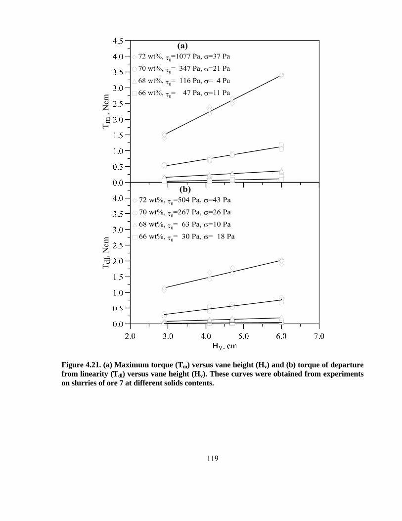
119
Figure 4.21. (a) Maximum torque (Tm) versus vane height (Hv) and (b) torque of departure from linearity (Tdl) versus vane height (Hv). These curves were obtained from experiments on slurries of ore 7 at different solids contents.
Tdl
,Ncm
Tm
,Ncm
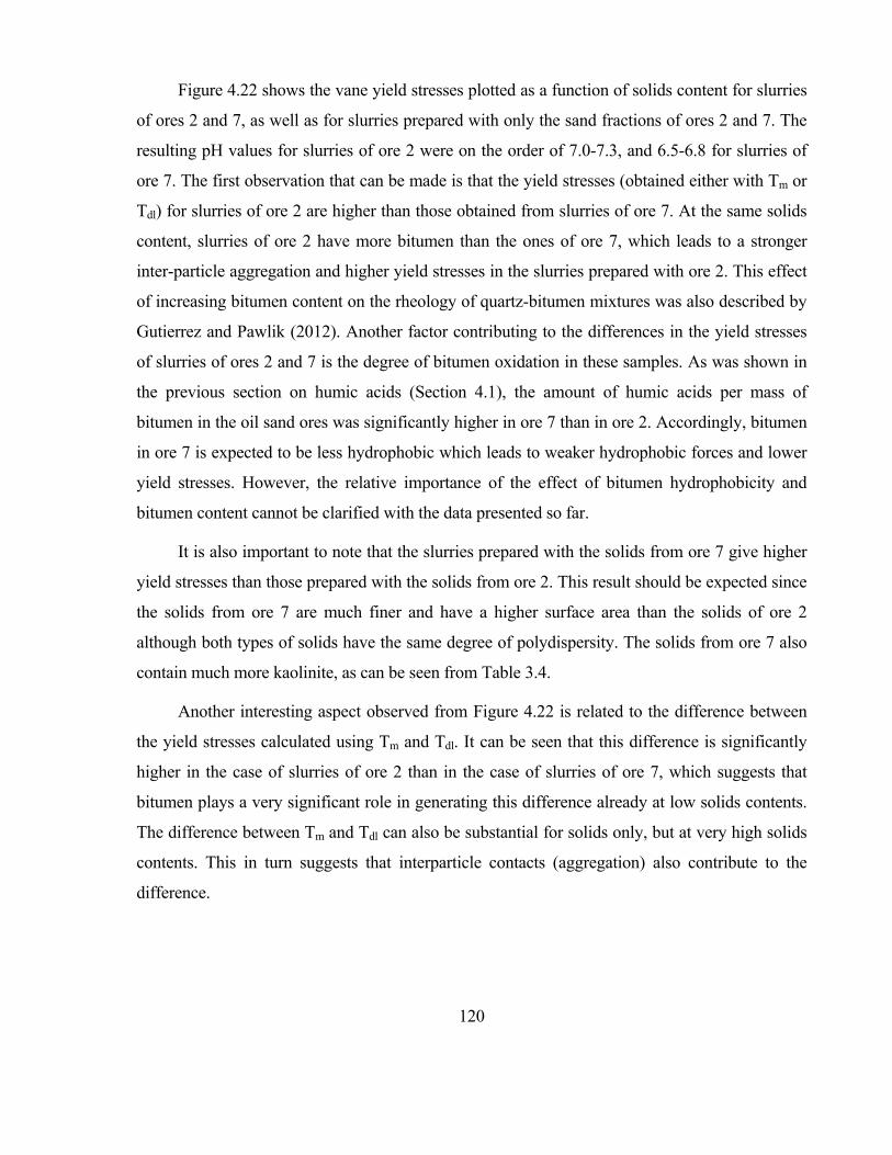
120
Figure 4.22 shows the vane yield stresses plotted as a function of solids content for slurries
of ores 2 and 7, as well as for slurries prepared with only the sand fractions of ores 2 and 7. The
resulting pH values for slurries of ore 2 were on the order of 7.0-7.3, and 6.5-6.8 for slurries of
ore 7. The first observation that can be made is that the yield stresses (obtained either with Tm or
Tdl) for slurries of ore 2 are higher than those obtained from slurries of ore 7. At the same solids
content, slurries of ore 2 have more bitumen than the ones of ore 7, which leads to a stronger
inter-particle aggregation and higher yield stresses in the slurries prepared with ore 2. This effect
of increasing bitumen content on the rheology of quartz-bitumen mixtures was also described by
Gutierrez and Pawlik (2012). Another factor contributing to the differences in the yield stresses
of slurries of ores 2 and 7 is the degree of bitumen oxidation in these samples. As was shown in
the previous section on humic acids (Section 4.1), the amount of humic acids per mass of
bitumen in the oil sand ores was significantly higher in ore 7 than in ore 2. Accordingly, bitumen
in ore 7 is expected to be less hydrophobic which leads to weaker hydrophobic forces and lower
yield stresses. However, the relative importance of the effect of bitumen hydrophobicity and
bitumen content cannot be clarified with the data presented so far.
It is also important to note that the slurries prepared with the solids from ore 7 give higher
yield stresses than those prepared with the solids from ore 2. This result should be expected since
the solids from ore 7 are much finer and have a higher surface area than the solids of ore 2
although both types of solids have the same degree of polydispersity. The solids from ore 7 also
contain much more kaolinite, as can be seen from Table 3.4.
Another interesting aspect observed from Figure 4.22 is related to the difference between
the yield stresses calculated using Tm and Tdl. It can be seen that this difference is significantly
higher in the case of slurries of ore 2 than in the case of slurries of ore 7, which suggests that
bitumen plays a very significant role in generating this difference already at low solids contents.
The difference between Tm and Tdl can also be substantial for solids only, but at very high solids
contents. This in turn suggests that interparticle contacts (aggregation) also contribute to the
difference.
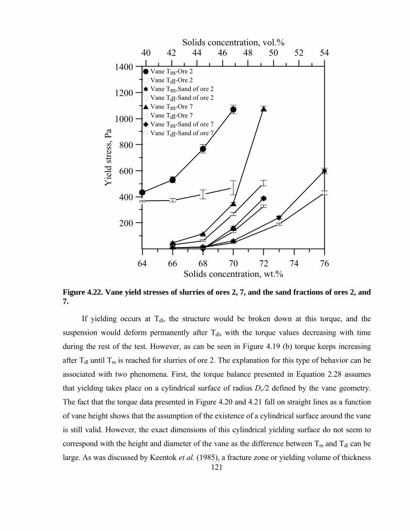
121
Figure 4.22. Vane yield stresses of slurries of ores 2, 7, and the sand fractions of ores 2, and 7.
If yielding occurs at Tdl, the structure would be broken down at this torque, and the
suspension would deform permanently after Tdl, with the torque values decreasing with time
during the rest of the test. However, as can be seen in Figure 4.19 (b) torque keeps increasing
after Tdl until Tm is reached for slurries of ore 2. The explanation for this type of behavior can be
associated with two phenomena. First, the torque balance presented in Equation 2.28 assumes
that yielding takes place on a cylindrical surface of radius Dv/2 defined by the vane geometry.
The fact that the torque data presented in Figure 4.20 and 4.21 fall on straight lines as a function
of vane height shows that the assumption of the existence of a cylindrical surface around the vane
is still valid. However, the exact dimensions of this cylindrical yielding surface do not seem to
correspond with the height and diameter of the vane as the difference between Tm and Tdl can be
large. As was discussed by Keentok et al. (1985), a fracture zone or yielding volume of thickness
64 66 68 70 72 74 76Solids concentration, wt.%
200
400
600
800
1000
1200
1400
Yie
ldst
ress
,Pa
Vane Tm-Ore 2Vane Tdl-Ore 2Vane Tm-Sand of ore 2Vane Tdl-Sand of ore 2Vane Tm-Ore 7Vane Tdl-Ore 7Vane Tm-Sand of ore 7Vane Tdl-Sand of ore 7
40 42 44 46 48 50 52 54Solids concentration, vol.%

122
is generated, and in this case the slurry yields not just on one plane but on a number of yielding
planes in the volume section located between Dv/2 and Dv/2+. According to this analysis, it can
be argued that slurry volumes located right on the cylindrical shearing surface defined by the
vane geometry yield at Tdl, after which additional layers of slurry farther away from the vane
start to yield, and the total torque still increases after Tdl. This advance of the yielding plane away
from the vane edges continues until the Tm is reached. Therefore, the results shown in Figure
4.22 can be analyzed following this concept of a yielding volume rather than of a single yielding
plane. For slurries of ore 2, which have high bitumen contents, the difference between Tm and Tdl
is large because interparticle aggregation and cohesion within the slurry are enhanced by the
bitumen phase, and propagation of shearing affects a larger volume of the slurries. In the absence
of bitumen, suspensions of solids alone do not exhibit a large difference between Tm and Tdl as
they yield along the vane surfaces. Even for solids only, this difference can be increased at higher
solids contents at which interparticle aggregation promotes the formation of extensive structuring
within the slurry. It is this internal slurry structure, whether produced by bitumen or by
interparticle aggregation that leads to yielding within a volume rather than on a well-defined
plane.
To verify how the deformation of the slurry propagates to planes away from the vane, a test
was carried out in which the vane was inserted only half way into slurries of ores 2 and 7. The
idea was to draw a white straight line on the surface of the slurry as shown in Figure 4.23, and to
follow the deformation and the position of the white line as a function of time and vane rotation
angle respect to the reference green line in Figure 4.23. The extension of the deformation of this
line from its zero time position gives a measure of how advanced is the propagation of shearing
generated by the vane. These results show that for the slurry of ore 2 the deformation of the white
line extends almost across the whole gap between the vane and the cup. In the case of the slurry
of ore 7, the deformation of the white line was localized to a section closer to the vane, and did
not extend to the outer cup. Figure 4.24 shows an schematic of extension of the deformation of
the time zero line for high and low bitumen ores. These visual observations qualitatively confirm
the concept that yielding of oil sand slurries does not take place at the cylindrical surface of the
vane, but rather over a distance farther away from the vane tips. Moreover, this distance appears
to increase with the bitumen content in the ore. Since high bitumen ores produce the largest

123
discrepancy between Tm and Tdl values, the difference between these two torque values seems to
result from the presence of bitumen. As noted earlier, slurries of solids from oil sand ores
basically yield at Tm = Tdl. It can be postulated that a sufficiently high amount of bitumen creates
a continuous highly viscous medium, compared to a low-viscosity aqueous phase, which
produces a solids-in-bitumen suspension of very strong cohesion and elasticity. As the vane
rotates in such a medium, the deformation extends/propagates much farther away from the vane
ends.
A key question as to which torque value represents the yield point will experimentally be
verified using other techniques for yield stress measurements.
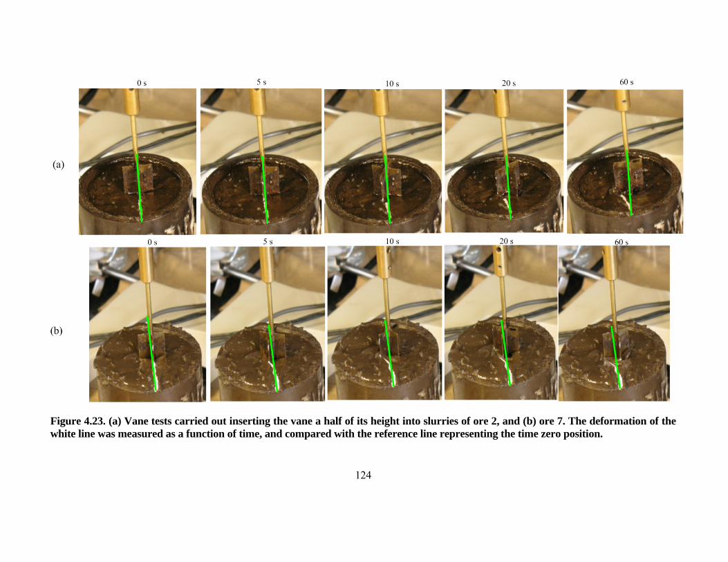
124
Figure 4.23. (a) Vane tests carried out inserting the vane a half of its height into slurries of ore 2, and (b) ore 7. The deformation of the white line was measured as a function of time, and compared with the reference line representing the time zero position.

125
Figure 4.24. Schematic of extension of the deformation of the time zero line for high and low bitumen ores.
4.2.2.2 Slump tests
Slump tests were performed on slurries prepared from ores 2 and 7, as well as using only
solids from those ores. Figures 4.25 (a), and (b) show pictures of the final shape of the samples
obtained from these experiments, at different solids concentrations. As can quite clearly be seen
from the figure, at the same solids content the slumps (“s” in Figure 2.12) obtained from tests on
slurries of ore 2 are smaller than the slumps obtained from experiments on slurries of ore 7. This
result again reveals the high degree of cohesion existing in the slurries prepared with ore 2. This
observation becomes more evident when the values of the yield stress obtained for these two
types of slurries are compared. As can be seen from Figure 4.26, the yield stresses of slurries of
ore 2 are significantly higher than the values obtained for slurries of ore 7, which is in agreement
with the results obtained from vane tests.
126
Figure 4.25. Pictures of slumped slurries of ores (a) 2, and (b) 7.
Figure 4.26 also displays the slump yield stresses for slurries prepared with the sand
fractions of ores 2, and 7. It can be seen that the yield stresses of slurries prepared from solids
from ore 7 are higher than those from solids of ore 2 which is also in agreement with the vane
tests. Similarly to the vane results, the high content of bitumen in ore 2 leads to a large difference
between the yield stress values for ore suspensions and the yield stresses of the sand suspensions.
At the same time, the effect of the much smaller bitumen content in ore 7 on the yield stress of
the sand and ore suspensions is rather small.

127
Figure 4.26. Comparison of yield stresses determined from slump tests for slurries of ores 2, and 7, as well as for slurries prepared with solids from ores 2 and 7.
4.2.2.3 Relaxation method
Attempts were made to use the relaxation method to measure the yield stress of
concentrated slurries for ores 2 and 7. The main objective of these tests was to obtain additional
data to verify and support the yield stress results obtained from the vane and slump tests.
However, the high bitumen content of ore 2 led to significant levels of bitumen build-up on the
rotating surfaces of the concentric cylinder rheometer, which made it impossible to perform
reliable and reproducible measurements. It is interesting to note that the build-up of bitumen on
the shearing surfaces of the rheometer was not observed during experiments on slurries of
artificial mixtures of fresh bitumen with fine quartz tested at 45 wt.% solids (Gutierrez and
64 65 66 67 68 69 70 71 72 73 74 75 76Solids concentration, wt.%
100
200
300
400
500
600
700
800
Yie
ldst
ress
,Pa
Ore 2Sand ore 2Ore 7Sand ore 7
40 41 42 43 44 45 46 47 48 49 50 51 52 53 54Solids concentration, vol.%
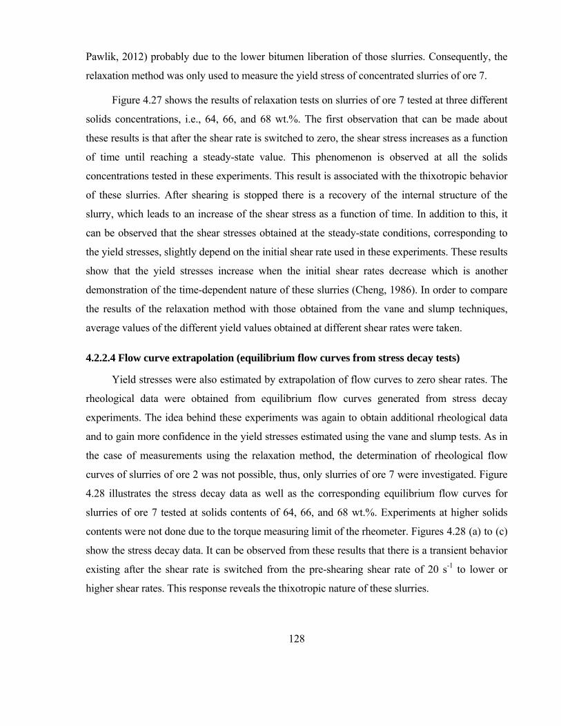
128
Pawlik, 2012) probably due to the lower bitumen liberation of those slurries. Consequently, the
relaxation method was only used to measure the yield stress of concentrated slurries of ore 7.
Figure 4.27 shows the results of relaxation tests on slurries of ore 7 tested at three different
solids concentrations, i.e., 64, 66, and 68 wt.%. The first observation that can be made about
these results is that after the shear rate is switched to zero, the shear stress increases as a function
of time until reaching a steady-state value. This phenomenon is observed at all the solids
concentrations tested in these experiments. This result is associated with the thixotropic behavior
of these slurries. After shearing is stopped there is a recovery of the internal structure of the
slurry, which leads to an increase of the shear stress as a function of time. In addition to this, it
can be observed that the shear stresses obtained at the steady-state conditions, corresponding to
the yield stresses, slightly depend on the initial shear rate used in these experiments. These results
show that the yield stresses increase when the initial shear rates decrease which is another
demonstration of the time-dependent nature of these slurries (Cheng, 1986). In order to compare
the results of the relaxation method with those obtained from the vane and slump techniques,
average values of the different yield values obtained at different shear rates were taken.
4.2.2.4 Flow curve extrapolation (equilibrium flow curves from stress decay tests)
Yield stresses were also estimated by extrapolation of flow curves to zero shear rates. The
rheological data were obtained from equilibrium flow curves generated from stress decay
experiments. The idea behind these experiments was again to obtain additional rheological data
and to gain more confidence in the yield stresses estimated using the vane and slump tests. As in
the case of measurements using the relaxation method, the determination of rheological flow
curves of slurries of ore 2 was not possible, thus, only slurries of ore 7 were investigated. Figure
4.28 illustrates the stress decay data as well as the corresponding equilibrium flow curves for
slurries of ore 7 tested at solids contents of 64, 66, and 68 wt.%. Experiments at higher solids
contents were not done due to the torque measuring limit of the rheometer. Figures 4.28 (a) to (c)
show the stress decay data. It can be observed from these results that there is a transient behavior
existing after the shear rate is switched from the pre-shearing shear rate of 20 s-1 to lower or
higher shear rates. This response reveals the thixotropic nature of these slurries.

129
Figure 4.27. Stress relaxation curves of slurries of ore 7. The data were obtained using the elongated fixture designed by Klein (1992).
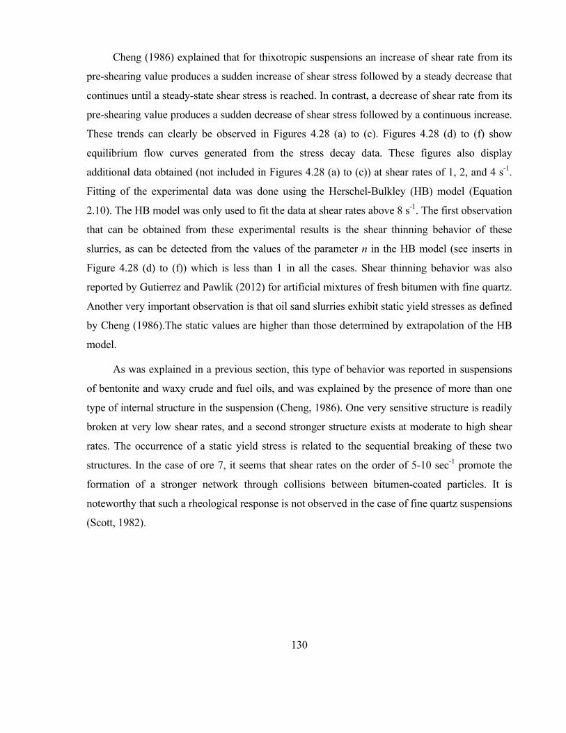
130
Cheng (1986) explained that for thixotropic suspensions an increase of shear rate from its
pre-shearing value produces a sudden increase of shear stress followed by a steady decrease that
continues until a steady-state shear stress is reached. In contrast, a decrease of shear rate from its
pre-shearing value produces a sudden decrease of shear stress followed by a continuous increase.
These trends can clearly be observed in Figures 4.28 (a) to (c). Figures 4.28 (d) to (f) show
equilibrium flow curves generated from the stress decay data. These figures also display
additional data obtained (not included in Figures 4.28 (a) to (c)) at shear rates of 1, 2, and 4 s-1.
Fitting of the experimental data was done using the Herschel-Bulkley (HB) model (Equation
2.10). The HB model was only used to fit the data at shear rates above 8 s-1. The first observation
that can be obtained from these experimental results is the shear thinning behavior of these
slurries, as can be detected from the values of the parameter n in the HB model (see inserts in
Figure 4.28 (d) to (f)) which is less than 1 in all the cases. Shear thinning behavior was also
reported by Gutierrez and Pawlik (2012) for artificial mixtures of fresh bitumen with fine quartz.
Another very important observation is that oil sand slurries exhibit static yield stresses as defined
by Cheng (1986).The static values are higher than those determined by extrapolation of the HB
model.
As was explained in a previous section, this type of behavior was reported in suspensions
of bentonite and waxy crude and fuel oils, and was explained by the presence of more than one
type of internal structure in the suspension (Cheng, 1986). One very sensitive structure is readily
broken at very low shear rates, and a second stronger structure exists at moderate to high shear
rates. The occurrence of a static yield stress is related to the sequential breaking of these two
structures. In the case of ore 7, it seems that shear rates on the order of 5-10 sec-1 promote the
formation of a stronger network through collisions between bitumen-coated particles. It is
noteworthy that such a rheological response is not observed in the case of fine quartz suspensions
(Scott, 1982).

131
Figure 4.28. (a-c) Stress decay results for slurries prepared with ore 7 at solids contents of 64, 66, and 68 wt.%. (d-f) Equilibrium flow curves generated from stress decay data These results were obtained using the elongated fixture.

132
4.2.2.5 Comparison of the yield stress values obtained using the vane, slump, relaxation,
and flow curve extrapolation methods
Figure 4.29 shows the yield stress values measured using the vane, relaxation, and
extrapolation methods for slurries of ore 7 in the solids concentration range from 64 to 68 wt.%.
These results show that, apart from the yield stress values calculated using Tm at 68 wt.% solids,
all the other results fall in a band of standard deviation of around ±20-25 Pa.
Figure 4.29. Yield stresses estimated using the slump, vane, flow curve extrapolation, and relaxation method for slurries of ore 7 prepared at solids concentrations between 64 and 68 wt.%.
Figure 4.30 shows the yield stresses obtained from vane and slump measurements for
slurries of ore 7 in the solids content range from 66 to 73 wt.%. These data show that the yield
stresses calculated from Tdl values agree with the values from slump tests over a wide range of

133
solids contents. However, the yield stresses calculated from Tm values are higher in the whole
range of solids content. As was already discussed, the process of interparticle aggregation and
networking in suspensions is promoted by higher solids contents and by higher amounts of
bitumen, and the plane of yielding generated by the vane propagates to positions away from the
cylindrical plane surrounding the vane, which creates the difference between the yield stresses
calculated with Tm and Tdl.
Figure 4.30. Yield stresses estimated using the slump, and vane methods for slurries of ore 7 prepared at solids concentrations between 66 and 73 wt.%.
Figure 4.31 shows the yield stresses obtained from vane and slump tests, for slurries of ore
2 in the solids content range from 64 to 70 wt.%. It can be seen that for slurries of this relatively
good processing ore the difference between the yield stress values calculated using Tm and Tdl is
rather high over the entire solids content range although the difference is more significant at
Yie
ldst
ress
,Pa

134
higher solids contents. Although the yield stresses calculated using Tdl are between 30 to 100 Pa
higher than those from slump tests, the experimental data suggest that the value of Tdl should be
taken to calculate the yield stress of oil sands slurries of high bitumen ores (good ores) since in
such a case the agreement between the yield stresses obtained from these two techniques is much
better.
Figure 4.31. Yield stresses estimated using the slump and vane methods for slurries of ore 2 prepared at solids concentrations between 64 and 70 wt.%.
Table 4.2 shows the summary of the data presented in Figures 4.29 to 4.31 including the
standard deviations of triplicate measurements.
64 65 66 67 68 69 70Solids concentration, wt.%
0
100
200
300
400
500
600
700
800
900
1000
1100
1200
Vane Tm
Vane Tdl
Slump
40 41 42 43 44 45 46 47 48 49 50Solids concentration, vol.%

135
Table 4.2. Numerical data of the results presented in Figures 4.29 to 4.31. is the standard deviation obtained from triplicates measurements.
Slurries ore 7 Vane Method Extrapolation of flow curve Relaxation
method Slump method Tm Tdl Dynamic yield stress Static yield stress
Solids o o o o o o wt% Pa Pa Pa Pa Pa Pa Pa Pa Pa Pa Pa Pa
76 690 16
73 568 12
72 1077 37 504 43 449 11
70 347 21 267 26 317 2
68 116 4 63 10 38 2 55 3 62 5 56 12
66 47 11 30 18 37 2 50 3 58 3
64 0 0 8 1 17 3 Slurries ore 2
Vane Method Slump test
Tm Tdl
Solids o o o
wt.% Pa Pa Pa Pa Pa Pa
70 1069 68 467 108 435 31
68 767 67 418 68 312 49
66 529 46 372 28 285 3
64 433 26 366 10 260 17
Figures 4.32 and 4.33 present the data obtained from vane and slump tests on slurries of the
sand fractions of ores 2 and 7, respectively. These results show that the yield stresses obtained
using Tdl agree well with the values obtained from slump tests in the whole range of solids
content. In contrast, the yield stresses calculated using Tm, only agree with the rest of the data in
the low range of concentrations, and significant departures can be observed at higher solids
contents.
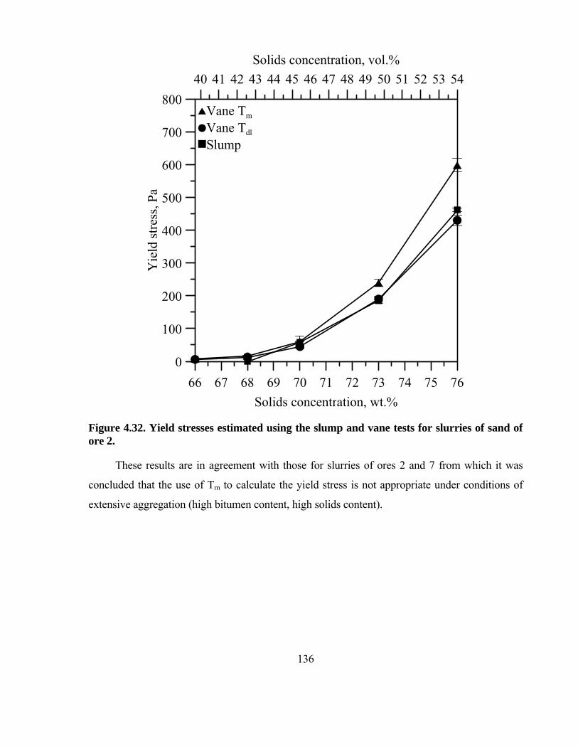
136
Figure 4.32. Yield stresses estimated using the slump and vane tests for slurries of sand of ore 2.
These results are in agreement with those for slurries of ores 2 and 7 from which it was
concluded that the use of Tm to calculate the yield stress is not appropriate under conditions of
extensive aggregation (high bitumen content, high solids content).
66 67 68 69 70 71 72 73 74 75 76
Solids concentration, wt.%
0
100
200
300
400
500
600
700
800
Yie
ldst
ress
,Pa
Vane Tm
Vane Tdl
Slump
40 41 42 43 44 45 46 47 48 49 50 51 52 53 54
Solids concentration, vol.%

137
Figure 4.33. Yield stresses estimated using the slump and vane tests for slurries of sand of ore 7.
Table 4.3 displays the numerical data plotted in Figures 4.32 and 4.33.
Yie
ldst
ress
,Pa

138
Table 4.3. Numerical data of the results presented in Figures 4.32 and 4.33. is the standard deviation obtained from triplicates measurements.
Slurries of sand of ore 2 Vane Method
Slump method Tm Tdl
Solids o o o wt% Pa Pa Pa Pa Pa Pa 76 598 41 430 33 462 10 73 239 22 190 17 185 17 70 60 2 45 4 58 37 68 16 3 13 2 0 0 66 8 1 6 3
Slurries of sand of ore 7 Vane Method
Slump method Tm Tdl
Solids o o o wt% Pa Pa Pa Pa Pa Pa 76 598 24 73 451 21 72 387 24 327 18 352 27 70 157 35 132 19 124 35 68 0 0 0 0 0 0
4.2.3 Effect of ore oxidation on the cohesiveness of oil sands slurries
The effect of bitumen oxidation was studied through experiments on slurries prepared with
an oxidized sample of ore 2. Ore oxidation was achieved by placing a larger sample of ore 2 in
an oven at 60 °C with air circulation for a period of one week. The temperature was relatively
low to prevent excessive evaporation of volatile bitumen components from the ore.
Attempts were made to perform vane and slump tests on the oxidized samples. However,
the reproducibility of the vane tests was very poor due to a run-off of water from the ore after
inserting the vane into the sample. The oxidation of bitumen seemed to increase the mobility of
water through the slurry matrix. As a result, dry and wet domains within the slurry could easily
be seen when the vane started to rotate. It can be seen from pictures in Figure 4.34 that the
slurries prepared using the oxidized sample of ore 2 showed slumps exhibiting a much lower
degree of cohesion. The data suggest that oxidation leads to a stronger dispersion of the slurry
components, which manifests itself in much lower yield stresses. The effect of artificial oxidation

139
on the hydrophobicity of bitumen can be correlated with the rheological behavior of oil sands
slurries. The results of alkali extraction tests presented in Figure 4.3 (a) showed that for ore 2
Abs520 was 0.23 (TOC= 102 mg/L). For the oxidized ore 2 this value was 0.29 (TOC=121
mg/L). The slump results presented in Figure 4.34 show that although the amount of humic acids
obtained from artificial oxidation of ore 2 was relatively low, their effect on
aggregation/cohesiveness, and consequently on rheology, was quite significant.
Figure 4.34. The slump behavior of slurries of ore 2, and of oxidized ore 2.
Since neither oxidized ore 2 nor fresh ore 2 was found to release humic acids under mild
conditions of pH and temperature, this drastic change in the rheological response of slurries of
oxidized ore 2 is unlikely to originate only from the dispersing (steric and electrostatic) action of
humic acids. Although the oxidized ore contains more humic acids compared to the fresh ore, as

140
shown in the alkali extraction tests, the humic matter appears to be bonded within the ore, most
likely within bitumen, and is not readily released into solution. It is reasonable to conclude that
the hydrophobicity of bitumen decreased as a result of oxidation, and the hydrophobic bonding of
various components of the suspension was much weaker. The hydrophobic/hydrophilic transition
on bitumen is clearly a critical factor in this result since the bitumen content in these two ore
samples (oxidized and fresh) is basically the same. Other ore properties, such as the particle size
distribution, were not affected by oxidation either. Therefore, the strong cohesion within the ore
was no longer observed and the slurry collapsed under the test conditions. Visual observations
during the test also indicated that water migration within the sample was much easier after
oxidation, and free water could clearly be seen accumulating at the slurry surface. This behavior
of water movement in the oxidized ore is actually very similar to the behavior of wet beach sand
under pressure, when drier areas of sand form as a result of free water flow away from the area
under pressure.
4.2.4 Effect of ore quality on the yield stress
The third set of experiments was aimed at studying the effect of ore quality on the yield
stress. In this case, slurries of ores 2, 3, 5, 6, and 7 were prepared at 70 wt.% solids and tested
through the vane and slump techniques. The results are shown in Figure 4.35. The first
observation that can be made is that slurries of high-bitumen ores (ores 2, 3, and 5) display
higher yield stress values than slurries prepared from low-bitumen ores, such as ores 6 and 7. It
should also be remembered that the relative amount of humic matter per mass of bitumen is
much higher in the case of ores 5, 6, and 7, so the hydrophobicity of bitumen also varies from ore
2 to ore 7. Bitumen in ore 2 can be expected to be more hydrophobic than bitumen in ore 7, and
as the slump test on oxidized ore 2 shows, the wettability of bitumen also contributes to the trend
in Figure 4.35.
Another important observation that can be obtained from Figure 4.35 is related to the
disagreement between Tm and Tdl. These results show that yield stresses calculated using Tdl are
in close agreement with the yield stress values obtained from the slump tests. However, a
significant disagreement is observed in the case of yield stresses calculated using Tm, with this
differences being more pronounced in the case of slurries of high-bitumen ores 2, 3, and 5. These
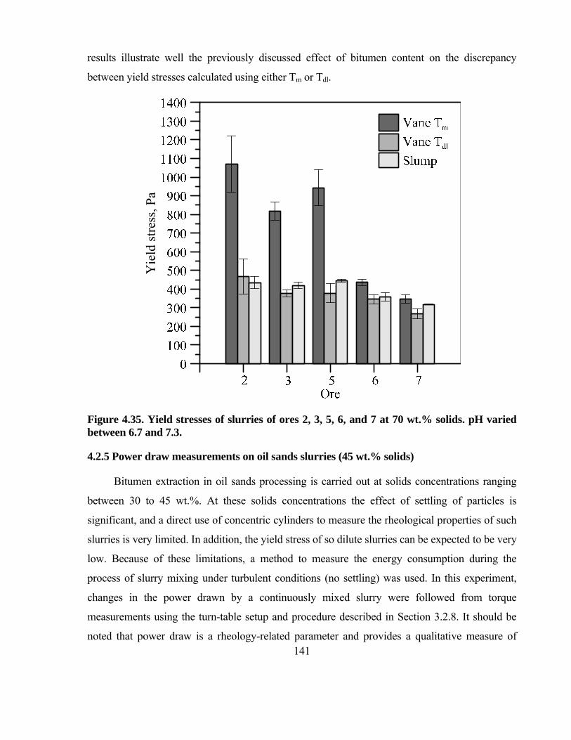
141
results illustrate well the previously discussed effect of bitumen content on the discrepancy
between yield stresses calculated using either Tm or Tdl.
Figure 4.35. Yield stresses of slurries of ores 2, 3, 5, 6, and 7 at 70 wt.% solids. pH varied between 6.7 and 7.3.
4.2.5 Power draw measurements on oil sands slurries (45 wt.% solids)
Bitumen extraction in oil sands processing is carried out at solids concentrations ranging
between 30 to 45 wt.%. At these solids concentrations the effect of settling of particles is
significant, and a direct use of concentric cylinders to measure the rheological properties of such
slurries is very limited. In addition, the yield stress of so dilute slurries can be expected to be very
low. Because of these limitations, a method to measure the energy consumption during the
process of slurry mixing under turbulent conditions (no settling) was used. In this experiment,
changes in the power drawn by a continuously mixed slurry were followed from torque
measurements using the turn-table setup and procedure described in Section 3.2.8. It should be
noted that power draw is a rheology-related parameter and provides a qualitative measure of
Yie
ldst
ress
,Pa

142
changes in slurry viscosity. These measurements were performed for 25 min in order to mimic
the residence time of slurries in the hydrotransport pipelines (~25 min). All experiments were
done at 45 wt.% solids, at different temperatures (20, 50 ºC), and pH (8.5, 10.0).
Figure 4.36 shows the results obtained from duplicate power draw measurements
performed on slurries of ores 2, 3, 5, and 7 tested at pH 8.5 and 50 ºC. It can be seen from these
four examples that the reproducibility of the power draw measurements was good. It was found
that the reproducibility of these measurements depended on several experimental variables. First,
the degree of agglomeration or presence of lumps in the original oil sands samples was found to
worsen the reproducibility of the tests. Because of this, all the samples were sieved through a 5.0
mm screen so that a uniform initial feed was obtained. A second experimental condition that had
to be carefully considered for good reproducibility was a proper control of pH. Sodium
hydroxide reacts with the sand as well as with the bitumen component of the ores. The products
of these chemical reactions are –SiO- groups on the surface of the sand grains, and surfactants
(and other organic matter) that are released from the bitumen component. Because of these
phenomena, any addition of NaOH to oil sands slurries produces an initial increase in pH which
is followed by a reduction of the OH- concentration which requires additional doses of NaOH in
order to maintain a constant pH value. These total additions of NaOH were estimated from
preliminary experiments to determine approximate dosages needed to achieve the required final
pH values so that changes in pH during the actual test were minimized.
It has to be noted that all the power draw measurements that will be presented in this
section were done in duplicates with levels of reproducibility similar to those presented in Figure
4.36, and average curves are used for analysis purposes.

143
Figure 4.36. Reproducibility of power draw measurements for slurries of ores 2, 3, 5, and 7 at 45 wt.% solids, pH 8.5, and 50 ºC. The average difference of these duplicates experiments was 0.28, 0.21, 0.24, and 0.35 kW/m3 for ores 2, 3, 5, and 7, respectively.
Figure 4.37 shows power draw measurements obtained from tests on slurries of ores 2, 3,
5, and 7 that were performed at pH values of 8.5 and 10, and temperatures of 20 and 50 ºC. In
general the power draw abruptly increases during the first 1-2 minutes of the experiments, after
which it decreases with time until an equilibrium steady-state value is reached at around 15-20
0 5 10 15 20 25Time, min
0
12
345
67
89
10
11 Ore 5Ore 5 (Duplicate)
01
234
56
789
1011
12Ore 2Ore 2 (Duplicate)
5 10 15 20 25Time, min
Ore 7Ore 7 (Duplicate)
Ore 3Ore 3 (Duplicate)
144
minutes. The sharp initial increase of power consumption observed in the first minutes of
experiments is larger for slurries of high bitumen ores as can be deduced from the peak values in
Figure 4.37. This result suggests that the initial jump in power draw can be related to bitumen
content in the slurries, and also the degree of hydrophobicity of bitumen. As the yield stress data
show, good processing ores with a high bitumen content are more aggregated in aqueous
suspensions than poor processing ores. Such aggregated systems require more power to initiate
flow under mixing.
Figure 4.37 shows that the power draw of slurries of ores 2, 3, and 5 decreased with an
increase in temperature. These results are in agreement with those presented by Gutierrez and
Pawlik (2012) who showed that the viscosity of synthetic oil sands slurries strongly decreased
with an increase in temperature. High temperatures enhance bitumen liberation/detachment from
the sand grains, thus effectively dispersing the slurry components, and consequently reducing
slurry viscosity. This effect on the overall slurry viscosity together with increased fluidity of
bitumen promote recession of bitumen from the sand grains and result in formation of bitumen
droplets in the slurry (Wallwork, 2003; Wallwork et al., 2004). Additionally, high temperatures
lead to an increase in interparticle repulsive forces, and decrease the adhesive forces existing
between bitumen and sand surfaces, which promotes dispersion and results in lower slurry
viscosities (Liu et al., 2002; Dai and Chung 1995). It is very interesting to note that neither
temperature nor pH had a significant effect on power draw for slurries of ore 7. Wallwork et al.
(2004) showed that for high fines ores with 30 vol.% of material below a size of 44 m, bitumen
liberation was more affected by temperature than for low fines ores. In the case of ore 7, the
solids are characterized by an extremely high fines content of 55.2 vol.%, and it is possible that
the attachment of bitumen to the fines is very strong and thus more difficult to modify by
temperature or pH.

145
Figure 4.37. Power draw measurements on slurries of ores 2, 3, 5, and 7 at pH 8.5 and 10, and temperatures of 20 and 50 ºC. Solids content was constant at 45 wt.%.
As far as the effect of pH is concerned, it can be seen from Figure 4.37 that the power draw
of slurries of ores 2, 3, and 5 decreased as pH increased from 8.5 to 10.0. These results can be
explained by dispersion/aggregation phenomena between the different ore components. It is
known that the zeta potentials of silica and bitumen show similar patterns with isoelectric points
of about 2 and 3, respectively (Dai and Chung, 1995). The silica and bitumen surfaces are
negatively charged at pH values higher than the isoelectric points. As was previously discussed,
0 5 10 15 20 25 30Time, min
0123456789
10111213
Pow
er,k
W/m
3
Ore 5pH 8.5, 20 oCpH 8.5, 50 oCpH 10, 20 oCpH 10, 50 oC
0123456789
1011121314
Pow
er,k
W/m
3
Ore 2pH 8.5, 20 oCpH 8.5, 50 oCpH 10, 20 oCpH 10, 50 oC
5 10 15 20 25 30Time, min
Ore 7pH 8.5, 20 oCpH 8.5, 50 oCpH 10, 20 oCpH 10, 50 oC
Ore 3pH 8.5, 20 oCpH 8.5, 50 oCpH 10, 20 oCpH 10, 50 oC

146
the surface charge of silica at pH values above 2 is determined by the chemical equilibrium given
by Equations 2.31 and 2.32. In this case the addition of a base (OH-) changes a fraction of the
neutral silanol groups (-SiOH) to negative groups (–SiO-) which renders the silica surface
negative. The surface charge of the bitumen/water interface can be explained by the dissociation
of carboxyl and other acidic groups naturally present in the bitumen (Takamura, 1985), with the
extent of this dissociation increasing at high pH. The final result of this increase in the negative
charge of bitumen and sand at high pH is an increase in repulsion between these two
components, which enhances bitumen liberation and dispersion of both bitumen and solids.
Slurries of ore 7 did not display any change in power draw as pH was changed from 8.5 to 10.
Due to the high levels of humic acids in ore 7, it is possible that the solids in this ore display
substantial hydrophobicity which leads to a strong attachment between bitumen and the solids in
the ore matrix. It seems that in this case the dispersing effect of pH on the bitumen-sand system
is overcome by hydrophobic attractive forces existing between bitumen and sand.
Figure 4.37 also shows that power consumptions in general decrease from ore 2 to ore 7. In
other words, slurries of low bitumen ores display the lowest values of power draw. One way to
see this more clearly is through the calculation of the area under the power draw curves which is
a measure of the energy consumed during the process of slurry mixing. Figures 4.38 shows the
energy consumed after 25 minutes of mixing for different combinations of pH and temperature. It
can be seen that in general the energy consumptions decrease from ore 2 to ore 7, results that
agree with yield stress measurements that showed that the low bitumen ores (poor ores)
displayed the lowest yield stresses. It is also very interesting to note that the pH and temperature
have a stronger effect on the energy consumption of slurries of high bitumen ores. The effects of
these two variables on slurries of ore 7 for example are not significant, while in the case of
slurries of ores 3, and 5 some changes can be observed but they are still small compared to the
changes for slurries of ore 2. This trend can be explained by gradual bitumen liberation when
temperature and pH are varied. Good ores respond better to the changes of the operating
conditions than poor ores. Because of this, an increase in temperature and pH leads to high
bitumen liberation in good ores, and lower slurry viscosities. It is also important to note that
suspensions of ore 7 consistently display the lowest energy consumptions regardless of
conditions, while suspensions of ore 2 give the highest values, even though ore 7 contains more
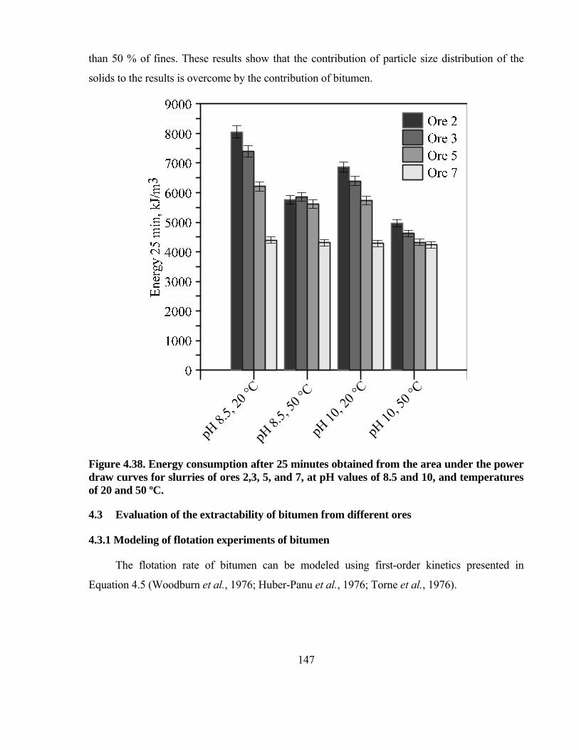
147
than 50 % of fines. These results show that the contribution of particle size distribution of the
solids to the results is overcome by the contribution of bitumen.
Figure 4.38. Energy consumption after 25 minutes obtained from the area under the power draw curves for slurries of ores 2,3, 5, and 7, at pH values of 8.5 and 10, and temperatures of 20 and 50 ºC.
4.3 Evaluation of the extractability of bitumen from different ores
4.3.1 Modeling of flotation experiments of bitumen
The flotation rate of bitumen can be modeled using first-order kinetics presented in
Equation 4.5 (Woodburn et al., 1976; Huber-Panu et al., 1976; Torne et al., 1976).

148
=-kC (4.5)
Where, C is the concentration of bitumen in the slurry, k is the flotation rate constant, and t
is the extraction time. Integrating Equation 4.5 with the initial condition that C=C0 at t=0,
Equation 4.6 is obtained.
=exp (4.6)
Then, the bitumen recovery R can be expressed as
= 1-exp (4.7)
Modeling of the experimental data of bitumen flotation can be supported by experimental
observations regarding the way in which bitumen is liberated and floated during this process. As
was explained in Section 3.2.9, flotation experiments on actual oil sand ores were done using
feed slurries that were conditioned for 25 min in the same turn-table set up that was used for
power draw measurements. After this, the flotation cell was removed from the turn-table, and
placed in the Denver flotation machine, where the slurry was re-suspended for 2 more minutes
before air was injected to the system. After 27 minutes of mixing, the presence of liberated
bitumen in the slurries was verified from visual observations that a layer of free bitumen formed
on the slurry surface. It was also observed that flotation of this liberated bitumen was very fast,
and the free bitumen layer disappeared after the first 30 seconds of flotation. Considering this
phenomenon, the process of bitumen flotation could be thought of as a process in which the total
amount of bitumen consists of two bitumen components, i.e., a fully-liberated bitumen
component characterized by a high flotation rate constant (kf), and a second poorly liberated

149
bitumen component of a low flotation rate constant (ks). In this case, the mass balance of the
bitumen in the slurry at time t is given by Equation 4.8.
t t + t (4.8)
Where, CT(t) is the total concentration of bitumen in the slurry at time t, and Cf(t) and Cs(t)
are the concentrations of the fast-floating and slow-floating bitumen components in the slurry at
time t, respectively. The change of concentrations of the fast- and slow-floating bitumen with
time, assuming a first order kinetics, can be expressed through Equation 4.9 and 4.10
respectively.
= 0 exp (4.9)
=s 0 exp (4.10)
Where, CT(0) is the total concentration of bitumen at time 0, and f and s are the relative
amounts (fractions) of the fast- and slow-floating bitumen in the slurry, respectively, so that
f+s=1.
It is very important to point out that the parameter f can be visualized as a factor
proportional to the degree of bitumen liberation from sand grains. It can provide an indication of
the relatives changes in bitumen liberation obtained under different operating conditions. This is
an interesting approach because the direct determination of bitumen liberation is a very difficult
experimental task.
Combining Equations 4.8, 4.9, and 4.10 an expression that correlates the total
concentration of bitumen in the slurry and the kinetic expressions for the concentration of the fast
and slow floating bitumen can be obtained (Equation 4.11).

150
0= exp + exp (4.11)
As can be seen, Equation 4.11 has four parameters, i.e., f, s, kf, and ks. One way to
determine the flotation rate constants of this equation is to fit the model to the data at two
extreme situations. The first one occurs at the beginning of the flotation process, when practically
all of the bitumen floated is the fast-floating liberated component. In this case, the contribution of
the second term (the slow-floating component) on the right hand side in Equation 4.11 can be
neglected, and the value of f can be assumed to be 1. Then kf can be obtained from the slope of a
graph of Ln[CT(t)/CT(0]) versus t. The other extreme situation takes place at the end of the
flotation experiment, when most if not all of the recovered bitumen is the slow-floating
component. In this case, the value of s can be assumed to be 1 and the flotation rate constant ks
can be obtained from the slope of a graph of Ln[CT(t)/CT(0)] versus t. Then, knowing the values
of kf and ks the values of f and s can be determined by minimization of the squared differences
between the model and the experimental data.
4.3.2 Flotation experiments with actual oil sands ores
4.3.2.1 Reproducibility of flotation experiments
Reproducibility of the flotation experiments was assessed by testing in duplicates two ores
of different processability, i.e., ores 2, and 5, under different conditions of pH and temperature,
i.e., pH 8.5 and 20 ºC, and pH 10.0 and 50 ºC. Figure 4.39 shows the obtained results. It can be
seen that the reproducibility of these experiments was very good with a maximum relative error
of around 8.9 %. In order to achieve this level of reproducibility, temperature adjustment,
conditioning time, control of pH, and homogeneity of the feed had to be consistently maintained
in all tests.

151
Figure 4.39. Reproducibility of flotation experiments for ores 2 and 5.

152
4.3.2.2 Bitumen extraction
Figure 4.40 shows the results of flotation experiments performed on slurries of ores 2, 3, 5,
and 7 at different conditions of pH and temperature. These flotation data were modeled using the
approach described in the previous section. The model fits to the data are shown as solid curves
in Figure 4.40. In addition, the total power consumption determined from power draw
measurements after 25 minutes of pre-conditioning in the turn-table set up is also indicated for
each set of conditions.
Analysis of the effects of pH and temperature on bitumen recovery reveals some
interesting features. It is observed that the effects of both pH and temperature on bitumen
extraction from ore 2 are of relatively similar magnitude, both parameters are equally important
in affecting the recovery of bitumen. In contrast, for ores 3 and 5 the effect of temperature is
significantly larger than the effect of pH. It is known that the hydrophobicity of fines in oil sands
ores is higher for ores of low bitumen and high fines contents (Bensebaa et al., 2000; Sparks et
al., 2003; Liu et al., 2004a; Dang-Vu et al., 2009). In addition to this, it was shown in the section
about humic acids that the concentrations of humic acids per gram of bitumen were higher in
ores 3 and 5 than in ore 2. Therefore, it should be expected that fines from ores 3 and 5 were
more hydrophobic than fines from ore 2 because of the adsorption of larger amounts of humic
acids on the sand fraction. In this case, because of the action of the attractive hydrophobic forces,
stronger adhesion between bitumen and fines can be expected in ores 3 and 5, leading to lower
bitumen liberation. Ores 3 and 5 contain more humic acids which lowers the cohesion within the
ore, as can be seen from the rheological data, but the hydrophobic nature of the solids prevents
bitumen liberation. In other words, pH results in dispersion of bitumen-coated fines, but does not
improve the detachment of bitumen from the fines. In this case, liberation and recovery can be
increased by increasing the fluidity of bitumen at higher temperatures, so the effect of
temperature is more significant than the effect of pH in ores 3 and 5 compared to ore 2.

153
Figure 4.40. Bitumen recovery from ores 2, 3, 5 and 7 with the corresponding values of energy consumption after 25 minutes of feed conditioning during power draw measurements.
Flotation data for ore 7 show that pH and temperature do not affect bitumen extraction
from this poor ore. This result agrees with the results from power draw measurements that
showed no effect of these two variables on the power draw of slurries of ore 7, which suggests
the existence of a correlation between extractability of bitumen and rheology of ore slurries. It
can be seen that in general bitumen recovery increases as the energy consumption during feed
0 1 2 3 4 5 6 7 8 9Time, min
pH 8.5, 20 °CpH 8.5, 50 °CpH 10.0, 20 °CpH 10.0, 50 °CFlotation model
0
10
20
30
40
50
60
70
80
90
100
0 1 2 3 4 5 6 7 8 9 10Time, min
pH 8.5, 20 °CpH 8.5, 50 °CpH 10.0, 20 °CpH 10.0, 50 °CFlotation model
10
20
30
40
50
60
70
80
90
100
pH 8.5, 20 °CpH 8.5, 50 °CpH 10.0, 20 °CpH 10.0, 50 °CFlotation model
Ore 2
pH 8.5, 20 °CpH 8.5, 50 °CpH 10.0, 20 °CpH 10.0, 50 °CFlotation model
Ore 3
Ore 5 Ore 7
4310 kJ/m3
4391 kJ/m3
4237 kJ/m3
4283 kJ/m3

154
conditioning decreases (ores 2, 3, and 5). This correlation can be explained by the fact that both
pH and temperature improve bitumen liberation from the sand grains (Dai and Chung, 1995;
Basu et al., 1996, Liu et al., 2003). Because of this, bitumen recovery increases as there is more
free bitumen dispersed in the slurry, and slurry viscosity decreases because the number of
bitumen-coated sand grains decreases.
It is interesting to note that the data in Figure 4.40 show that for ore 2 bitumen recovery
was the highest at pH 10. However, the results of contact angle measurements presented in
Figure 4.10 showed that the hydrophobicity of bitumen decreased as pH increased, which should
lead to a weak attachment between air bubbles and bitumen droplets. Schramm and Smith (1985)
explained that at high pH, the concentration of surfactants in solution increases as a result of the
increase in pH. This effect was also observed in this research, as discussed in section 4.1. These
surfactants adsorb on the air bubbles and lower the interfacial tension at the air-bitumen interface,
facilitating the formation of an air-in-bitumen dispersion of rather low density (Schramm and
Smith 1985). It appears that such a mechanism contributes to the high level of bitumen flotation
at high pH.
The changes in bitumen liberation obtained as a result of changes in pH and temperature
can also be detected from the variation of the parameter f of the flotation model. Table 4.4
summarizes the model parameters. It can be seen that f increases with pH and temperature for
ores 2, 3, and 5. In the case of ore 2, the effect of temperature on f is slightly higher than the
effect of pH. In contrast, for ores 3 and 5 the effect of temperature is clearly larger than the effect
of pH.
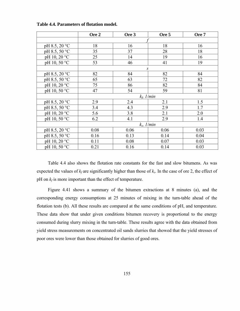
155
Table 4.4. Parameters of flotation model.
Ore 2 Ore 3 Ore 5 Ore 7 f
pH 8.5, 20 °C 18 16 18 16 pH 8.5, 50 °C 35 37 28 18 pH 10, 20 °C 25 14 19 16 pH 10, 50 °C 53 46 41 19
s pH 8.5, 20 °C 82 84 82 84 pH 8.5, 50 °C 65 63 72 82 pH 10, 20 °C 75 86 82 84 pH 10, 50 °C 47 54 59 81
kf, 1/min pH 8.5, 20 °C 2.9 2.4 2.1 1.5 pH 8.5, 50 °C 3.4 4.3 2.9 1.7 pH 10, 20 °C 5.6 3.8 2.1 2.0 pH 10, 50 °C 6.2 4.1 2.9 1.4
ks, 1/min pH 8.5, 20 °C 0.08 0.06 0.06 0.03 pH 8.5, 50 °C 0.16 0.13 0.14 0.04 pH 10, 20 °C 0.11 0.08 0.07 0.03 pH 10, 50 °C 0.21 0.16 0.14 0.03
Table 4.4 also shows the flotation rate constants for the fast and slow bitumens. As was
expected the values of kf are significantly higher than those of ks. In the case of ore 2, the effect of
pH on kf is more important than the effect of temperature.
Figure 4.41 shows a summary of the bitumen extractions at 8 minutes (a), and the
corresponding energy consumptions at 25 minutes of mixing in the turn-table ahead of the
flotation tests (b). All these results are compared at the same conditions of pH, and temperature.
These data show that under given conditions bitumen recovery is proportional to the energy
consumed during slurry mixing in the turn-table. These results agree with the data obtained from
yield stress measurements on concentrated oil sands slurries that showed that the yield stresses of
poor ores were lower than those obtained for slurries of good ores.

156
Figure 4.41. (a) Bitumen recovery after 8 min of flotation, and (b) energy consumption after 25 min of conditioning of the feed as determined with the turn-table set-up.

157
Figure 4.42 shows plots of bitumen recovery as a function of the Abs520 obtained from
alkali extraction tests for ores 2, 3, 5, and 7. It can be seen that the total bitumen recovery after 8
minutes of flotation decreases with an increase in the Abs520 in all the cases. These results show
that the high levels of humic acids present in the ores of low processability correlate very well
with the low bitumen recoveries obtained from these ores. The amount of humic acids leached
from the ores is a measure of the degree of bitumen weathering/oxidation, and higher amounts of
humic acids should be associated with higher hydrophilicity of bitumen and therefore with
reduced bitumen recovery. These oxidation products on the bitumen surface effectively act like
depressants of bitumen flotation.
The results in Figure 4.42 show that the parameter Abs520 correlates very well the
extraction data. Most of the literature on oil sands generally focuses on the effect of fines and
bitumen content on extraction, but it is clear that there is a very strong relationship with the
amount of humic acids leached from the ores. High-fines and low-bitumen ores appear to be
more degraded/oxidized compared to high-bitumen and low-fines ores. It has to be pointed out
that when the extraction data are plotted as a function of either the fines or the bitumen contents
the correlations are not so pronounced. The fact that the parameter Abs520 was the only ore
property that correlated well with the extraction data under all the conditions strongly suggests
that the quantification of humic acids in the ores is essential in analyzing the rheology and
extraction results.
Figure 4.43 shows the recovery of solids obtained from the flotation tests. The first
observation that can be made is that under given conditions of pH and temperature, the recovery
of solids from ore 7 is higher than that from the other samples. As was explained in the literature
review humic acids due to their complex and heterogeneous nature are capable of interacting
with a large variety of materials including clays and minerals (Fairhurst and Warwick, 1998;
Jones and Bryan, 1998). The adsorption of humic acids on the sand fraction then renders the
solids hydrophobic. As a result bitumen liberation from the sand is low and the sand remains
coated with bitumen even at conditions of high pH and temperature.
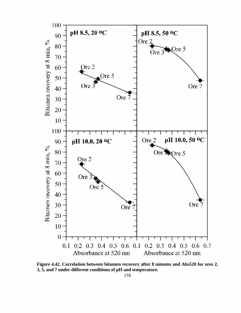
158
Figure 4.42. Correlation between bitumen recovery after 8 minutes and Abs520 for ores 2, 3, 5, and 7 under different conditions of pH and temperature.

159
This analysis agrees with the observations by Czarnecki et al. (2005) who suggested that
sand particles can be coated by organic coatings of humic matter that render the particles
hydrophobic and oil-wet. Therefore, in the case of ore 7 the particles of sand are hydrophobic not
only because of the adsorption of humic acids but mainly because they are coated by bitumen
which explains the high solids recoveries from ore 7. This mechanism can be corroborated from
the data of bitumen and solids recovery from ore 7 presented in Figures 4.41 and 4.43. If these
data are compare for ore 7 it is possible to find that bitumen recovery is high when solids
recovery is high which suggests that bitumen and solids float together. However, in the case of
ore 2, bitumen recovery is high when solids recovery is low which shows that in this case
bitumen floats separately.
Figure 4.43. Solids recovery after 8 min of flotation under different pH and temperature conditions.
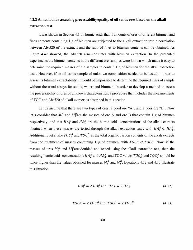
160
4.3.3 A method for assessing processability/quality of oil sands ores based on the alkali
extraction test
It was shown in Section 4.1 on humic acids that if amounts of ores of different bitumen and
fines contents containing 1 g of bitumen are subjected to the alkali extraction test, a correlation
between Abs520 of the extracts and the ratio of fines to bitumen contents can be obtained. As
Figure 4.42 showed, the Abs520 also correlates with bitumen extraction. In the presented
experiments the bitumen contents in the different ore samples were known which made it easy to
determine the required masses of the samples to contain 1 g of bitumen for the alkali extraction
tests. However, if an oil sands sample of unknown composition needed to be tested in order to
assess its bitumen extractability, it would be impossible to determine the required mass of sample
without the usual assays for solids, water, and bitumen. In order to develop a method to assess
the processability of ores of unknown characteristics, a procedure that includes the measurements
of TOC and Abs520 of alkali extracts is described in this section.
Let us assume that there are two types of ores, a good ore “A”, and a poor ore “B”. Now
let’s consider that and are the masses of ore A and ore B that contain 1 g of bitumen
respectively, and that and are the humic acids concentrations of the alkali extracts
obtained when these masses are tested through the alkali extraction tests, with ≪ .
Additionally let’s take and as the total organic carbon contents of the alkali extracts
from the treatment of masses containing 1 g of bitumen, with ≪ . Now, if the
masses of ores and are doubled and tested using the alkali extraction test, then the
resulting humic acids concentrations and , and TOC values and should be
twice higher than the values obtained for masses and . Equations 4.12 and 4.13 illustrate
this situation.
2 and 2 (4.12)
2 and 2 (4.13)

161
These equations reveal that, as is significantly higher than , the absolute increase
in humic acids concentration associated with the increase in mass for ore B should be
significantly higher than the increase observed for ore A. The same conclusion applies to the
TOC data. In other words, an increase in humic acids and TOC concentrations as a result of
increasing mass of ore in the alkali extraction tests should be higher for poor ores than for good
ores.
In order to experimentally verify these observations, additional alkali extraction tests were
performed on each of the eight ores. In these tests, three different masses of each ore were tested,
i.e., 5.5, 10.0, and 33.3 g. These values were chosen assuming that the bitumen content in oil
sand ores varies between 3 and 18 wt.% so the required ore to contain 1 g of bitumen are 33.3,
and 5.5 g for 3 wt.% and 18 wt.%, respectively.
Figure 4.44 shows the results of the TOC and Abs520 of the extracts obtained from tests on
the oil sands ores. As can be seen from this graph, three points are presented for each ore, with
the numerical values of these data points increasing as the mass of ore used for the alkali
extraction tests increases in the order 5.5, 10.0, and 33.3 g. The data for each ore seem to fall on
straight lines, as could be expected. The first important observation from Figure 4.44 is that good
processing ores tend to produce the TOC and Abs520 data located on the left-lower side of the
graph. In contrast, the data from poor processing ores run towards the upper right corner of the
graph. Additionally, the progressive increase of mass produced in these experiments generates a
stronger increase of TOC and Abs520 for the extracts obtained from poor processing ores than
for those from good processing ores. In this analysis, Abs520 can be visualized as a parameter
that characterizes the amount of humic acids in the alkali extracts, while the TOC as a parameter
that characterizes all the organics leached from the ores.
Another way to analyze these results is through the determination of the areas under the
curves presented in Figure 4.44. An increase in Abs520 and TOC obtained from the same
proportional increase of ore mass depends on ore quality, i.e, poor ores produce higher
proportional increases in TOC and Abs520 than good ores. Then, the area under the curve of a
graph of TOC versus Abs520 could be interpreted as a factor proportional to the value of Abs520
per gram of bitumen as was presented in Figure 4.1. As seen from Figure 4.45, the area under the
TOC-Abs520 curve increases as the quality of the ore decreases. High quality ores (high
162
bitumen, low fines, high bitumen extractability) should produce low areas under the curves, in
contrast to low quality ores (low bitumen, high fines, low bitumen extractability).
Figure 4.44. TOC versus Abs520 from alkali extraction tests on for ore masses of 5.5, 10, and 33.3 g.
The proposed experimental procedure simply involves subjecting 2-3 samples of different
masses of the same ore (between about 5 and 34 g) to the alkali extraction test, measuring the
Abs 520 and TOC of the extracts, and comparing the resulting line/curve with the analogous set
of data for a known ore. In this way, an assessment of ore processability with respect to the
reference ore can quickly be made. It is worth stressing that no other ore properties need to be
determined.
Based on this test, it is also possible to classify different types of ores by comparing the
curves generated from the values of TOC and Abs520. The analysis of the data obtained from the
tests on the eight ore samples used in this work indicates that good ores (low fines, high bitumen,
Tot
alor
gani
cca
rbon
,mg/
L

163
such as ore 1) should produce areas under the TOC-Abs520 curves lower than 20 mg/L, average
ores (ores 2-5) between 30 and 50 mg/L, and for poor ores (ores 6-8) the area should be higher
than 70 mg/L.
Figure 4.45. Area under the curve of TOC versus Abs520 shown in Figure 4.44.
Are
aun
der
curv
eT
OC
vsA
bs52
0,m
g/L

164
5 Conclusions
The alkali extraction test originally developed to determine the oxidation of bituminous
metallurgical coals is an effective tool to assess the degree of oxidation of oil sands ores. Oil
sands ores respond to the test in the same manner as bituminous coals with different degrees of
oxidation. The intensity of the characteristic yellow-brown color of the alkali extracts, which
originated from the presence of humic acids, was a function of the quality of the ore samples.
Good processing ores produced very clear extracts while poor ores gave extracts with a yellow-
brown color. The absorbance of the alkali extracts spectra at 520 nm (Abs520) was found to be a
good parameter to quantify the relative amounts of humic substances in ores of different quality.
This parameter correlated very well with the dimensionless ratio of the fines content (-44 m size
fraction) to the bitumen content which also revealed a relationship with the processability of the
ores. Good ores contained the lowest amount of humic acids per mass of bitumen, while the ratio
of humic acids to bitumen was much higher for poor ores. As a result, a very good correlation
was further observed between Abs520 and bitumen recovery from the tested ores.
The application of the alkali extraction test to determine the degree of oxidation of oil
sands ores was supported by FTIR measurements. These results demonstrated that the intensity
(absorbance) of the peaks associated with aliphatic hydrocarbons (2,800-2,980 cm-1) decreased as
the Abs520 increased, and at the same time, the intensity of the peak from carbonyl groups
(1600-1700 cm-1) increased. These trends demonstrated that the amount of oxygen-containing
compounds on the bitumen surface, including humic acids, was proportional to the Abs520 of the
alkali extracts. Therefore, the alkali extraction test not only quantifies the amount of humic acids
in the ores, but also provides a measure of bitumen oxidation. It appears that bitumen in poor
processing ores can be characterized by a higher content of oxygen functional groups compared
to bitumen in good ores.
Although good ores did not release substantial amounts of humic acids, it was found from
total organic carbon (TOC) measurements that alkali extracts from good ores still contained high
levels of organic matter. A closer comparison between the UV/Visible spectra of the alkali
extracts obtained from the tested ores and spectra of solutions of commercial humic acids
indicated that the total organic carbon content of the extracts of good ores primarily originated

165
from compounds other than humic acids, while the organic matter released by poor ores was
dominated by humic acids. The fact that the organics leached from good ores do not resemble
humic acids suggests that these ores primarily release ionic surfactants, which is consistent with
other literature data about the leaching of surfactants by oil sand ores.
Humic acids are difficult to leach from oil sands under the conditions of the bitumen
extraction process (pH 8.5, 50 °C). In fact, the leaching of organic matter under these mild
conditions is insignificant compared to the amount of organics obtained from alkali extraction
tests. The experimental data suggest that the oxidation products that produce humic acids in the
alkali extraction test are strongly bonded with the ores components, most likely with bitumen,
and that humic acids do not occur in oil sands ores as free, easily leachable chemical compounds.
Wettability studies showed that the contact angle of water on the fresh bitumen surface
decreased with pH. Bitumen was found to be most hydrophobic at low pH, and most hydrophilic
at high pH. This wetting behavior of fresh bitumen can be explained by changes in the
dissociation of residual oxygen functional groups on the bitumen surface. In an acidic
environment, weakly acidic groups are fully protonated and uncharged so the electrostatic
contribution to the work of adhesion of water to bitumen disappears. Under neutral and alkaline
conditions, the full dissociation of the surface oxygen groups in combination with small
quantities of surfactants leached from bitumen render the bitumen surface more hydrophilic.
Through the same mechanism, the hydrophobicity of bitumen significantly decreases when the
bitumen surface becomes oxidized and enriched in oxygen containing groups, although the
oxidation process does not generate significant amounts of humic acids leachable by alkali
extraction. The contact angle of water on fresh bitumen significantly decreases in the presence of
humic acids only at low pH, while under neutral and alkaline conditions (pH 7-10) the effect of
humic acids on bitumen wettability is very weak. Under neutral and alkaline conditions,
electrostatic repulsion between the negatively charged bitumen surface and the anionic humic
acids prevents humic acids adsorption onto bitumen, and consequently changes in bitumen
wettability are not pronounced in the presence of humic acids. At pH 3, the bitumen surface is
almost uncharged and the now protonated humic acids more readily adsorb on the bitumen
surface and render it hydrophilic. The overall effect of added humic acids on bitumen wettability
is actually lower than the effect of artificial oxidation of bitumen, which suggests that humic

166
acids make bitumen hydrophilic if they are part of internal/surface bitumen structure in the form
of oxygen-containing compounds, but not when they are added as free chemicals, particularly
under neutral and alkaline pH conditions. The effect of free humic acids on the rheology of
artificial ore slurries and on bitumen extractability from the ores was also minor, which
highlights the importance of bitumen wettability in rheology and extractability.
The rheology of oil sands slurries depends on the bitumen content of the oil sands slurries
as well as on the quality or processability of the ores from which the corresponding slurries are
prepared. At the same solids content, slurries prepared from good processing ores display higher
yield stresses, and higher viscosities compared to those prepared from poor processing ores.
Bitumen acts as a high-viscosity binder increasing the internal cohesion of the slurry although the
strength of the internal slurry structure, as measured by the yield stress of the slurry, depends on
the hydrophobicity of bitumen. Breakdown of heavy hydrocarbons in bitumen could not be ruled
out, but experimental observations showed that bitumen remained highly viscous after oxidation.
Even mild oxidation of an otherwise good quality ore drastically lowers the yield stress of a
concentrated slurry prepared from the oxidized ore. As a result, a low amount of bitumen with a
higher amount of oxygen functional groups in poor processing ores does not generate high yield
stresses and has a small overall influence on slurry rheology.
Observations made during the vane test indicated that concentrated slurries of high-
bitumen ores yielded within a volume of the slurry that extended far beyond the cylindrical
surface defined by the geometrical dimensions of the vane. This propagation of the yielding
plane beyond vane dimensions was much less pronounced in concentrated slurries of low
bitumen ores. Therefore, it was proposed that this unusual behavior of concentrated oil sands
slurries was caused by the presence of bitumen, which at sufficiently high concentrations
created a continuous high-viscosity medium of high elasticity. As a result, the calculation of
the yield stress from torque-vs-time curves generated using the vane method required a careful
analysis of the shape of the curves. It was found that the torque value at the point of departure
from linearity (Tdl) along the initial part of the curve, rather than the maximum torque value on
the curve (Tm), gave yield stress values that agreed very well with those obtained with other
measuring techniques. The difference between the maximum torque on the torque-time curve
and the torque at the point of departure from linearity was large for high bitumen ores which

167
suggested that this difference was produced by bitumen. Additional vane tests on slurries
prepared only from the solids extracted from the ores showed that the difference between Tm
and Tdl was very small and either Tm or Tdl could be used to assess the yield stress. However,
even for those bitumen-free slurries the difference between Tm and Tdl increased with
increasing solids content, which suggested that the difference between those two torque values
generally originated from extensive aggregation between particles within a concentrated slurry.
Under such conditions the Tdl value rather than Tm should be used for calculating yield stresses
from the vane method.
Power draw measurements during mixing of oil sand suspensions were found to
qualitatively correlate with the yield stress data. In all cases, the power draw abruptly increased
during the first 1-2 minutes of mixing producing a sharp peak. This initial fast increase in
power draw resulted from breaking of the internal slurry structure after which power draw
steadily decreased with time as the slurry components gradually became dispersed. The
maximum power draw at the peak was the highest for high-bitumen ores whose concentrated
slurries were also characterized by a high yield stress. Increasing pH and temperature resulted
in a decrease of the total power draw for high-bitumen ores. Since power draw for slurries of
low-bitumen ores was not affected by temperature and pH, the decrease in power consumption
at higher pH and temperature for slurries of high-bitumen ores was most likely caused by
enhanced bitumen liberation and dispersion during mixing.
The recovery of bitumen from oil sand ores correlated very well with the parameter
Abs520 of the alkali extracts produced from the ores. High bitumen recovery was achieved for
ores characterized by a low absorbance value of the extract, while low bitumen recoveries were
obtained for ores producing a high absorbance value in the alkali extraction test. Since Abs520
is a measure of the amount of humic acids leached from the ores, the results suggested that the
presence of humic acids in the ores was a very significant factor in bitumen extraction. The
presence of high amounts of humic acids in oil sands ores led to low bitumen recoveries and
the action of humic acids was basically that of a depressant. In combination with the total
organic carbon content in the extracts, Abs520 can be used for predicting the processability of
a given ore.

168
The recovery of bitumen during the extraction process can readily be modeled using first-
order kinetics equations and assuming that the total amount of bitumen in the system can be
represented by two bitumen components, i.e., a fully-liberated bitumen fraction, f, characterized
by a high flotation rate constant (kf), and a poorly-liberated bitumen fraction, s, of a low flotation
rate constant (ks). In this case, f and s can also be defined as the relative amounts (fractions) of
the fast- and slow-floating bitumen in the slurry, respectively. The parameter f of the flotation
model is related to the degree of bitumen liberation from the sand particles. It was found that this
parameter significantly increased with pH and temperature for good-average ores, but not for
poor ores.

169
6 Recommendations for future work
A more extended experimental program aimed at obtaining additional data from alkali
extraction tests on ores of good processability (high bitumen and low fines contents) should be
performed. In this thesis, only one good processing ore sample containing less than 10 % of fines
was tested with all the other ores containing more than 20 % of fines.
Additional work should be carried out in order to determine the partition of humic acids in
the oil sands ores. The analysis of bitumen and sand samples obtained through separation using
toluene indicates that the humic acids in the original ores samples remained in the sand fraction
after filtration of the toluene organic solution. However, it is not possible to determine whether
these humic substances were originally in the sand or the bitumen. In general, characterization of
all organic matter leachable from different types of oil sands ores deserves further studies. Some
of these chemicals are beneficial to bitumen extraction but some of them (e.g., humic acids) have
a negative impact. Also, the presence of organic dispersing agents on fine solids most likely
affects the flocculation of the resulting tailings, and this aspect has never been researched. From
this point of view, adsorption of humic acids on solids from oil sands and the effect of humic
acids on the wettability of bitumen should be studied in greater detail. For such studies, it is
recommended to use humic acids obtained directly from the alkali extraction test on a real ore
rather than commercially-available synthetic humic acids.
It would be also very interesting to make efforts to correlate the parameter f of the flotation
model proposed in this thesis with the degree of bitumen liberation from the sand particles. This
task of course will require firstly obtaining a reliable technique to determine bitumen liberation.
The effect of other organic polymers and surfactants on the kinetics of bitumen liberation should
also be investigated.
The infinite gap approach appears to be a very reliable technique for measuring the
rheology of concentrated oil sands slurries. The technique avoids all the experimental issues
related to bitumen build-up and plugging of the gaps of rotational viscometers. The method can
also be used in the field. However, the method does not address the issue of the settling of solids
from dilute oil sands slurries. Therefore, the method should be evaluated in greater detail for
obtaining entire equilibrium flow curves from the raw torque-rotational speed data.
170
Bibliography
Alberta Chamber of Resources, 2004, “Oil sands technology roadmap-Unlocking the potential”.
Angove, M.J., Johnson, B.B., Wells, J.D., 1997, “Adsorption of cadmium (II) on kaolinite”, Colloids and Surfaces A: Physicochemical and Engineering Aspects, Vol. 126, 137-147.
Barnes, H.A., Walters, K., 1985, “The yield stress myth?”, Rheologica Acta, 24, 323-326.
Barnes, H.A., Hutton, J.F., Walters, K., 1989, “An introduction to rheology”, Elsevier, Amsterdam.
Barnes, H.A., Carnali, J.O., 1990, “The vane-in-cup as a novel rheometer geometry for shear thinning and thixotropic materials”, Journal of Rheology, 34(6), 841-866.
Barnes, H.A., Nguyen, Q.D., 2001, “Rotating vane rheometry: a review”, Journal of Non-Newtonian Fluid Mechanics, 98, 1-14.
Basu, S., Nandakumar, K., Masliyah, J.H., 1996, “A study of oil displacement on model surfaces”, Journal of Colloid and Interface Science, 182, 82-94.
Basu, S., Nandakumar, K., Masliyah, J.H., 1998a, “A visual study of high grade oil sand disintegration process”, Journal of Colloid and Interface Science, 205, 201-203.
Basu, S., Kanda, W.C., Nandakumar, K., Masliyah, J.H., 1998b, “Effect of hydrophobic and hydrophilic clays on bitumen displacement by water on a glass surface”, Ind. Eng. Chem. Res., 37, 959-965.
Basu, S., Kanda, W.C., Nandakumar, K., Masliyah, J.H., 1998c, “Effect of NaCI and MIBC/kerosene on bitumen displacement by water on a glass surface”, Colloids and Surfaces A: Physicochemical and Engineering Aspects, 136, 71-80.
Basu, S., Nandakumar, K., Lawrence, S., Masliyah, J.H., 2004, “Effect of calcium ion and montmorillonite clay on bitumen displacement by water on a glass surface”, Fuel, 83, 17-22.
Behzadfar, E., Hatzikiriakos, S.G., 2012, “Viscoelastic properties and constitutive modelling of bitumen”, Fuel (In Press). Available online 25 December 2012.
Bensebaa, F., Kotlyar, L.S., Sparks, B.D., Chung, K.H., 2000, “Organic coated solids in Athabasca bitumen: characterization and process implications”, The Canadian Journal of Chemical Engineering, 78, 610-616.
Bingham, E.C., 1922, “Fluidity and Plasticity”, McGraw-Hill, New York, p. 217.
Bingham, E.C., 1930, “Rheology definitions make progress”, Journal of Rheology, 1(5), 507-516.
171
Boger, D.V., 1977, “Demonstration of upper and lower Newtonian fluid behavior in a pseudoplastic fluid”, Nature, 265, 126-128.
Boylu, F., Dincer, H., Atesok, G., 2004, “Effect of coal particle size distribution, volume fraction and rank on the rheology of coal-water slurries”, Fuel Processing Technology, 85, 241-250.
Brandenburg, U., Lagaly, G., 1988, “Rheological properties of sodium montmorillonite dispersions”, Applied Clay Science, 3, 263-279.
British Standard Glossary of Rheological Terms, BS 5168: 1975, British Standards Institution (1975)
Bulmer, J.T., Starr, J., 1979, “Syncrude analytical methods for oil sand and bitumen processing”, The Alberta Oil Sands Technology and Research Authority, 46-52.
Carreau, P.J., 1972, “Rheological equations from molecular network theories”, Transactions of the Society of Rheology, 16(1), 99-127.
Carreau, P.J., De Kee, D., 1979a, “Review of some useful rheological equations”, Canadian Journal of Chemical Engineering, 57, 3-15.
Carreau, P.J., De Kee, D., 1979b, “An analysis of the viscous behavior of polymeric solutions”, Canadian Journal of Chemical Engineering, 57, 135-140.
Casson, N., 1959, “A flow equation for pigment-oil suspensions of the printing ink type”, in “Rheology of Dispersed Systems”, C.C.Mill (Ed.), Pergamon Press, New York, 84.
Charrie-Duhaut, A., Lemoine, S., Adam, P., Connan, J., Albrecht, P., 2000, “Abiotic oxidation of petroleum bitumens under natural conditions”, Organic Geochemistry, 31, 977-1003.
Cheng, D.C-H., 1986, “Yield stress: A time-dependent property and how to measure it”, Rheologica Acta, 25, 542-554.
Cheng, D.C-H., 1971, “The interpretation of cone-and-plate viscometer loop experiments”, Journal of Physics E: Scientific Instruments, 4, 693-699.
Christensen, G., 1991, “Modelling the flow of fresh concrete: the slump test”, PhD thesis, Princeton University.
Claesson, P.M., Blom, C.E., Herder, P.C., Ninham, B.W., 1986, “Interactions between water-stable hydrophobic Langmuir-Blodgett monolayers on mica”, Journal of Colloid and Interface Science, 114(1), 234-242.
Clark, K.A., 1929, “The separation of the bitumen from Alberta bituminous sands”, Can. Inst. Min. Metall., Bull. 22, 1385-1395.

172
Clark, K.A., Pasternack, D.S., 1932, “Hot water separation of bitumen from Alberta bituminous sand”, Ind. Eng. Chem., 24, 1410-1416.
Clark, K.A., 1944, “Hot-water separation of Alberta bituminous sand”, CIM Transactions, XLVII (47), 257-274.
Clark, K.A., 1950, “The Hot-water washing method for recovering of oil from the Alberta tar sands”, Canadian Oil and Gas Industries, 3, 46-50.
Clark, K.A., 1966, “Athabasca oil sands-Fundamentals affecting development”, Canadian Petroleum, 7, 18-21.
Cokelet, G.R., Merrill, E.W., Gilliland, E.R., 1963, “The Rheology of Human Blood-Measurement Near and at Zero Shear Rate”, Transactions of the Society of Rheology, 7, 303-317.
Cox, H.W., Macosko, C.W., 1974, “Viscous dissipation in die flows”, AIChE Journal, 20(4), 785-795.
Cullen, P.J., O’Donnell, C.P., Houska, M., 2003, “Rotational rheometry using complex geometries-A review”, Journal of Texture Studies, 34, 1-20.
Cross, M.M., 1965, “Rheology of Non-Newtonian fluids: a new flow equation for pseudoplastic systems”, Journal of Colloid Science, 20, 417-437.
Czarnecki, J., Radoev, B., Schramm, L. Slavchev, R., 2005, “On the nature of Athabasca oil sands”, Advances in Colloid and Interface Science, 114-115, 53-60.
Dai, Q., Chung, K.H., 1995, “Bitumen-sand interaction in oil sand processing”, Fuel, 74[12], 1858-1864.
Dai, Q., Chung, K.H., 1996, “Hot water extraction process mechanism using model oil sands”, Fuel, 75[2], 220-226.
Dang-Vu, T., Jha, R., Wu, S., Tannant, D., Masliyah, J., Xu, Z., 2009, “Wettability determination of solids isolated from oil sands”, Colloids and Surfaces A: Physicochemical and Engineering Aspects, 337, 80-90.
De Kee, D., Turcotte, G., Fildey, K., Harrison, B., 1980, “New method for the determination of yield stress”, Journal of Texture Studies, 10, 281-288.
Dealy, J.M., Giacomin, A.J., 1988, “Sliding plate and sliding cylinder rheometers”. In: Collyer, A. A., and Clegg, D.W., eds. Rheological Measurement. Elsevier, London, pp. 383-404.
Derjaguin, B.V., Landau, L., 1941, Acta Physicochim. USSR, 633.

173
Drelich, J., Long, J., Yeung, A., 2007, “Determining surface potential of the bitumen-water interface at nanoscale resolution using atomic force microscopy”, The Canadian Journal of Chemical Engineering, 85, 625-634.
Einstein, A., 1906, Annalen der Physik., 19, 289-306.
Elfarissi, F., Pefferkorn, E., 2000, “Kaolinite/humic acid interaction in the presence of aluminium ion”, Colloids and Surfaces A: Physicochemical and Engineering Aspects, 168, 1-12.
Ellis, S.B., 1929, Thesis, Lafayette College, Pa.
Eyring, H., 1936, “Viscosity, plasticity, and diffusion as examples of absolute reaction rates”, The Journal of Chemical Physics, 4, 283-291.
Fagan, M.E., Zukoski, C.F., 1997, “The rheology of charge stabilized silica suspensions”, Journal of Rheology, 41[2], 373-397.
Fairhurst, A.J., Warwick, P., 1998, “The influence of humic acid on europium-mineral interactions”, Colloids and Surfaces A: Physicochemical and Engineering Aspects, 145, 229-234.
Farris, R.J., 1968, “Prediction of the viscosity of multimodal suspensions from unimodal viscosity data”, Transactions of the Society of Rheology, 12(2), 281-301.
Farrow, J.B., Horsley, R.R., Meagher, L., Warren, L.J., 1989, “The effect of alkali and alkaline earth cations on the rheology of concentrated quartz suspensions”, Journal of Rheology, 33[8], 1213-1230.
Fidleris, V., Whitmore, R.L., 1961, “The physical interaction of spherical particles in suspensions”, Rheologica Acta, Band 1, 4-6, 573-580.
Firth, B.A., Nicol, S.K., 1981, “The influence of humic materials on the flotation of coal”, International Journal of Mineral Processing, 8, 239-248.
Fisher, D.,T., Clayton, S.A., Boger, D.V., Scales, P.J., 2007, “The bucket rheometer for shear stress-shear rate measurement of industrial operation”, Journal of Rheology, 51[5], 821-831.
Fowkes, F.M., 1964, “Attractive forces at interfaces”, Industrial and Engineering Chemistry, 56(12), 40.
Fowkes, F.M., 1967, “Attractive forces at solid liquid interfaces”, in Wetting, Society of Chemical Industry Monograph no. 25, Gordon and Breach, New York, p. 3.
Franks, G.V., Zhou, Z., Duin, N.J., 2000, “Effect of inter-particle forces on shear thickening of oxide suspensions”, Journal of Rheology, 44[4], 759-779.

174
Franks, G.V., 2002, “Zeta potential and yield stresses of silica suspensions in concentrated monovalente electrolytes: isoelectric point shift and additional attraction”, Journal of Colloid and Interface Science, 249, 44-51.
Friesen, W.I., Dabros, T., Kwong, T., 2004, “A bench-scale study of conditioning behavior in oil sand slurries”, The Canadian Journal of Chemical Engineering, 82, 743-751.
Fuerstenau, M.C., Palmer, B.R., 1976, “Anionic flotation of oxides and silicates”, in Flotation, A.M. Gaudin Memorial Volume, Vol. I, M.C. Fuerstenau, ed., AIME, New York, 149-196.
Gamboa, C., Olea, A.F., 2006, “Association of cationic surfactants to humic acid Effect on the surface activity”, Colloids and Surfaces A: Physicochemical and Engineering Aspects,278, 241-245.
Genc, A.M., 2009, “Power draw measurements as a method of characterization of particle aggregation”, M.A.Sc. Thesis, The University of British Columbia, Vancouver, Canada.
Goldsmith, H.L., Mason, S.G., 1962, “The flow of suspensions through tubes I. Single spheres, rods, and discs”, Journal of Colloid Science, 17, 448-476.
Goldsmith, H.L., Mason, S.G., 1967, “The Microrheology of Dispersions”, Proc. 4th Int. Congr. On Rheology, Providence, Rhode Island, F.R. Eirich, ed, John Wiley and Son, New York, 85-250.
Green, R.G., Griskey, R.G., 1968a, “Rheological behavior of dilatant (shear-thickening) fluids. Part I. Experimental and data”, Transactions of the Society of Rheology, 12(1), 13-25.
Green, R.G., Griskey, R.G., 1968b, “Rheological behavior of dilatant (shear-thickening) fluids. Part II. Mechanism and theory”, Transactions of the Society of Rheology, 12(1), 27-37.
Gutierrez, L.E., 2009, “Probing mineral-bitumen liberation using rheological measurements”, M.A.Sc. Thesis, The University of British Columbia, Vancouver, Canada.
Gutierrez, L.E., Pawlik, M., 2012, “Influence of pH and temperature on the rheology of aqueous quartz-bitumen suspensions”, Journal of Rheology, 56, 687-706.
Gu, G., Zhou, Z., Xu, Z., Masliyah, J., 2003, “Role of fine kaolinite clay in toluene-diluted bitumen/water emulsion”, Colloids and Surfaces A: Physicochem. Eng. Aspects, Vol. 215, 141-153.
Hepler, L.G., Smith, R.G., 1994, “The Alberta oil sands: industrial procedures for extraction and some recent fundamental research”, AOSTRA Technical Publication Series-Alberta Oil Sands Technology and Research Authority, Edmonton Canada, 14.
Herschel, W.H., Bulkley, R., 1926, Proc. Amer. Soc. Test. Matls., 26(II), 621.
175
Hoffman, R.L., 1992, “Factors affecting the viscosity of unimodal and multimodal dispersions”, Journal of Rheology, 36(5), 947-965.
Hooshiar, A., Uhlik, P., Kaminsky, H.W., Shinbine, A., Omotoso, O., Liu, Q., Ivey, D.G., Etsell, T.H., 2010, “High resolution transmission electron microscopy study of clay mineral particles from streams of simulated water based bitumen extraction of Athabasca oil sands”, Applied Clay Science, 48, 466-474.
Hu, Y., Wei, S., Hao, J., Miller, J.D., Fa, K., 2005, “The Anomalous Behavior of Kaolinite with Dodecyl Amine Collector as Explained from Crystal Structure Considerations”, International Journal of Mineral Processing, Vol. 76, 163-172.
Huber-Panu, I., Ene-Danalache, E., Cojocariu, D.G., 1976, “Mathematical models of batch and continuous flotation”, in Flotation, A.M. Gaudin Memorial Volume, Vol. II, M.C. Fuerstenau, ed., AIME, New York, 675-724.
Hupka, J., Miller, J.D., Cortez, A., 1983, “Importance of bitumen viscosity in the hot water processing of domestic tar sands”, Mining Eng., 35, 1635-1641.
Ignasiak, T.M., Zhang, Q., Kratochvil, B., Maitra, C., Montgomery, D.S., Strausz, O.P., 1985, “Chemical and mineral characterization of the bitumen-free Athabasca oil sands related to the bitumen concentration in the sand tailings from the Syncrude batch extraction test”, AOSTRA Journal of Research, 2(1), 21-35.
Ishida, N., Sakamoto, M., Miyahara, M., higashitani, K., 2000, “Attraction between hydrophobic surfaces with and without gas phase”, Langmuir, 16, 5681-5687.
Israelachvili, J.N., Pashley, R.M., 1984, “Measurement of the hydrophobic interaction between two hydrophobic surfaces in aqueous electrolyte solutions”, Journal of Collloid and Interface Science, 98(2), 500-514.
Jacobesen, R.T., “The determination of the flow curve of a plastic medium in a wide gap rotational viscometer”, Journal of Colloid and Interface Science, 48(3), 437-441, 1974.
Johnson, S.B., Russell, A.S., Scales, P.J., 1998, “Volume Fraction Effects in Shear Rheology and Electroacoustic Studies of Concentrated Alumina and Kaolin Suspensions”, Colloids and Surfaces A: Physicochem. Eng. Aspects, Vol. 141, 119-130.
Jones, M.N., Bryan, N.D., 1998, “Colloidal properties of humic substances”, Advances in Colloid and Interface Science, 78, 1-48.
Joye, D.D., 2003, “Shear rate and viscosity corrections for a Casson fluid in cylindrical (Couette) geometries”, Journal of Colloid and Interface Science, 267, 204-210.
Kaminsky, H.A.W., Etsell, T.H., Ivey, D.G., Omotoso, O., 2008, “Characterization of heavy minerals in the Athabasca oil sands”, Minerals Engineering, 21, 264-271.

176
Kasongo, T., Zhou, Z., Xu, Z., Masliyah, J., 2000, “Effect of clays and calcium ions on bitumen extraction from athabasca oil sands using flotation”, Canadian Journal of Chemical Engineering, 78, 674-681.
Kasongo, T., 2006, “Role of fine clays and ionic species in bitumen extraction from oil sand ores using the hot water extraction process”, PhD Thesis, The University of Alberta, Edmonton, Canada.
Kelessidis, V.C., Maglione, R., 2008, “Shear rate corrections for Herschel-Bulkley fluids in Couette geometry”, Applied Rheology, 18(3), 1-11.
Keentok, M., 1982, “The measurement of the yield stress of liquids”, Rheologica Acta, 21, 325-332.
Keentok, M., Milthorpe, J.F., O’Donovan, E., 1985, “On the shearing zone around rotating vanes in plastic liquids: theory and experiment”, Journal of Non-Newtonian Fluid Mechanics, 17, 23-35.
Kessick, M.A., 1979, “Structure and properties of oil sands clay tailings”, The Journal of Canadian Petroleum Technology, January-March, 49-52.
Klein, B., 1992, “Rheology and stability of magnetite dense media”, PhD Thesis, The University of British Columbia, Vancouver, Canada.
Klein, B., Laskowski, J.S., Partridge, S.J. 1995, “A new viscometer for rheological measurements on settling suspensions”, Journal of Rheology, 39[5], 827-840.
Kotlyar, L.S., Sparks, B.D., Kodama, H., 1985, “Isolation of inorganic matter-humic complexes from Athabasca oil sands”, AOSTRA Journal of Research, 2(2), 103-111.
Kotlyar, L.S., Ripmeester, J.A., Sparks, B.D., Montgomery, D.S., 1988, “Characterization of oil sands solids closely associated with Athabasca bitumen”, Fuel, 67, 808-814.
Kotlyar, L.S., Ripmeester, J.A., Sparks, B.D., 1990, “Isolation and characterization of various types of organic matter in oil sands tailings sludge”, Fuel, 69, 1522-1526.
Krieger, I.M., Maron, S.H., 1951, “Rheology of synthetic latex. I. Test of some flow equations”, Journal of Colloid Science, 6, 528-538.
Krieger, I.M., Maron, S.H., 1952, “Direct determination of the flow curves of nonNewtonian fluids”, Journal of Applied Physics, 23, 147-149.
Krieger, I.M., Elrod, H., 1953, “Direct determination of the flow curves of non-Newtonian fluids. II. Shearing rate in the concentric cylinder viscometer”, Journal of Applied Physics, 24, 134-136.
Krieger, I.M., Maron, S.H., 1954, “Direct determination of the flow curves of non-Newtonian fluids. III. Standardized treatment of viscometric data”, Journal of Applied Physics, 25, 72-75.

177
Krieger, I.M., Dougherty, T.J., 1959, “A mechanism for Non-Newtonian flow in suspensions of rigid spheres”, Transactions of the society of rheology, III, 137-152.
Krieger, I.M., Woods, E., 1966, “Direct determination of the flow curves of nonNewtonian fluids. IV. Parallel plane rotational viscometer”, Journal of Applied Physics, 37, 4703-4704.
Krieger, I.M., 1968, “Shear rate in the Couette viscometer”, Transactions of the Society of Rheology, 12(1), 5-11.
Lang, E.R., Rha, C., 1981, “Determination of the yield stress of hydrocolloid dispersions”, Journal of Texture Studies, 12, 47-62.
Lapidot, M., Mellgren, O., 1968, “Conditioning and flotation of ilmenite ore”, Trans. IMM, C77, 149-165.
Laskowski, J.S., 2001, “Coal Flotation and Fine Coal Utilization”, Elsevier Publication
Laskowski, J.S., Sirois, L.L., Moon, K.S., 1986, “Effect of humic acids on coal flotation, Part I: Coal flotation selectivity in the presence of humic acid”, Coal Preparation, Vol. 3, 133-154.
Laun, H.M., 1988, in Proceedings of the 10th International Congress on Rheology, Vol. 1, Uhlherr, P.H.T., Ed., Sydney.
Lecomte du Nou¨y, P., 1919, “A new apparatus for measuring surface tension”, J. Gen. Physiol., Vol. 1, 521–524.
Lee, J.D., So, J.H., Yang, S.M., 1999, “Rheological behavior and stability of concentrated silica suspensions”, Journal of Rheology, 43[5], 1117-1140.
Leja, J., 1982, “Surface chemistry of froth flotation”, Plenum Press, New York and London.
Lewis, T.B., Nielsen, L.E., 1968, “Viscosity of dispersed and aggregated suspensions of spheres”, Transactions of the Society of Rheology, 12(3), 421-443.
Liu, Q., Laskowski, J.S., 1988, “Effect of humic acids on coal flotation, Part II: The role of pH”, SME Annual Meeting, Phoenix, AZ, Preprint 88-31.
Liu, J., Zhou, Z., Xu, Z., Masliyah, J., 2002, “Bitumen–Clay Interactions in Aqueous Media Studied by Zeta Potential Distribution Measurement”, Journal of Colloid and Interface Science, 252, 409-418.
Liu, J., Xu, Z., Masliyah, J., 2003, “Studies on bitumen-silica interactions in aqueous solutions by atomic force microscopy”, Langmuir, 19, 3911-3920.
Liu, J., Xu, Z., Masliyah, J., 2004a, “Interaction between Bitumen and Fines in Oil Sands Extraction System: Implication to Bitumen Recovery”, The Canadian Journal of Chemical Engineering, 82, 655-666.
178
Liu, J., Xu, Z., Masliyah, J., 2004b, “Role of Fine Clays in Bitumen Extraction from Oil Sands”, AICHE Journal, 50[8], 1917-1927.
Liu, J., Xu, Z., Masliyah, J., 2005, “Colloidal forces between bitumen surfaces in aqueous solutions measured with atomic force microscope”, Colloids and Surfaces A: Physicochem. Eng. Aspects, 260, 217-228.
Long, J., Drelich, J., Xu, Z., Masliyah, J.H., 2007, “Effect of Operating Temperature on Water‑Based Oil Sands Processing”, The Canadian Journal of Chemical Engineering, 85, 726-738.
Lowenhaupt, D.E., Gray, R.J., 1980, “The alkali-extraction test as a reliable method of detecting oxidized metallurgical coal”, International Journal of Coal Geology, 1, 63-73.
Luckham, P.F., Ukeje, M.A., 1999, “Effect of particle size distribution on the rheology of dispersed systems”, Journal of Colloid and Interface Science, 220, 347-356.
Ma, X., Pawlik, M., 2005, “Effect of alkali metal cations on adsorption of guar gum onto quartz”, Journal of Colloid and Interface Science, 289, 48-55.
Mackley, M.R., 1988, “Capillary rheometry”. In: Collyer, A. A., and Clegg, D.W., eds. Rheological Measurement. Elsevier, London, pp. 1-23.
Macosko, C.W., 1994, Rheology: Principles, Measurements and Aplications. VCH Publishers, Inc., New York.
Magnin, A., Piau, J.M., 1987, “Shear rheometry of fluids with a yield stress”, Journal of Non-Newtonian Fluid Mechanics, 23, 91-106.
Majid, A., Ripmeester, J.A., 1990, “Isolation and characterization of humic acids from Alberta oil sands and related materials”, Fuel, 69, 1527-1535.
Majid, A., Sparks, B.D., Ripmeester, J.A., 1991, “Characterization of solvent-insoluble organic matter isolated from Alberta oil sands”, Fuel, 70, 78-83.
Majid, A., Sparks, B.D., Ripmeester, J.A., 1992, “Isolation and characterization of humic matter from Syncrude sludge pond tailings”, Fuel, 71, 165-168.
Majid, A., Sparks, B.D., 1996, “Role of hydrophobic solids in the stability of oil sands fine tailings”, Fuel, 75(7), 879-884.
Majid, A., Sparks, B.D., Ripmeester, J.A., 2000a, “Characterization of humic acids from sludge pond solids”, National Research Council Canada Document NRCC No. 32540, 1354-1360.
Majid, A., Sparks, B.D., Ripmeester, J.A., 2000b, “Characterization of insoluble organic matter associated with clay minerals from Syncrude sludge pond tailings”, National Research Council Canada Document NRCC No. 32541, 1348-1353.
179
Maron, S.H., Madow, B.P., Krieger, I.M., 1951, “Rheology of synthetic latex. II. Concentration dependence of flow in type V GR-S latex”, Journal of Colloid Science, 6, 584-591.
Maron, S.H., Madow, B.P., 1953, “Rheology of synthetic latex. III. Concentration dependence of flow in type III GR-S latex”, Journal of Colloid Science, 8, 130-136.
Maron, S.H., Fok, S.M., 1955, “Rheology of synthetic latex. V. Flow behavior of low-temperature GR-S latex”, Journal of Colloid Science, 10, 482-493.
Maron, S.H., Levy-Pascal, A.E., 1955, “Rheology of synthetic latex. VI. The flow behavior of neoprene latex”, Journal of Colloid Science, 10, 494-503.
Masliyah, J., Kwong, T., Seyer, F., 1981, “Theoretical and experimental studies of a gravity separation vessel”, Industrial and Engineering Chemistry Process Design and Development, 20, 154-160.
Masliyah, J., Zhou, Z.J., Xu, Z., Czarnecki, J., Hamza, H., 2004, “Understanding water-based bitumen extraction from athabasca oil sands”, The Canadian Journal of Chemical Engineering, 82, 628-654.
Masutani, G., Stenstrom, M.K., 1984, “A review of surface tension measuring techniques, surfactants, and their implications for oxygen transfer in wastewater treatment plants”, Water Research Program, School of Engineering and Applied Science, University of California, Los Angeles.
Metzner, A.B., 1985, “Rheology of suspensions in polymeric liquids”, Journal of Rheology, 29(6), 739-775.
Mewis, J., 1979, “Thixotropy-A general review”, Journal of Non-Newtonian Fluid Mechanics, 6, 1-20.
Mikula, R.J., Munoz, V.A., Wamg, N., Bjornson, B., Cox, D., Moisan, B., Wiwchar, K., 2003, “Characterization of bitumen properties using microscopy and near infrared spectroscopy: processability of oxidized or degraded ores”, Journal of Canadian Petroleum Technology, 42(8), 50-54.
Mikula, R.J., Munoz, V.A., Omotoso, O., 2008, “Correlation of natural surfactant partitioning and bitumen recovery in oil sands extraction”, The Petroleum Society 59th Annual Meeting, Canadian International Petroleum Conference/SPE Gas Technology Symposium, Jun 17 - 19, 2008, Calgary, Alberta.
Mills, P., Rubi, J.M., Quemada, D., 1980, “Suspension Flow”, in, “Rheology Vol.2: Fluids”, Eds. G. Astarita et al., Plenum Press, 639-643.
Morgan, R.J., 1968, “A study of the phenomenon of rheological dilatancy in an aqueous pigment suspension”, Transactions of the Society of Rheology, 12(4), 511-533.

180
Mossop, G.D., 1980, “Geology of the Athabasca oil sands”, Science, 207, 145-152.
National Energy Board, 2006, “Canada’s Oil Sands, Opportunities and challenges to 2015: an update”.
Nguyen, Q.D., Boger, D.V., 1983, “Yield stress measurement for concentrated suspensions”, Journal of Rheology, 27(4), 321-349.
Nguyen, Q.D., Boger, D.V., 1985, “Direct yield stress measurement with the vane method”, Journal of Rheology, 29(3), 335-347.
Painter, P., Starsinic, M., Coleman, M., 1985, “Determination of functional groups in coal by Fourier Transform Interferometry”, Chapter 5 in “Fourier Transform Infrared Spectroscopy”, J.R. Ferraro, L.J. Basile (Eds), Vol. 4, p. 169, Academic Press.
Pal, R., Masliyah, J., 1990, “Rheology of oil in water emulsions with added solids”, The Canadian Journal of Chemical Engineering, Vol. 68, 24-28.
Parker, J.L., Claesson, P.M, Attard, P., 1994, “Bubbles, cavities, and the long-ranged attraction between hydrophobic surfaces”, J. Phys. Chem., 98, 8468-8480.
Parkinson, C., Matsumoto, S., Sherman, P., 1970, “The influence of particle-size distribution on the apparent viscosity of non-Newtonian dispersed systems”, Journal of Colloid and Interface Science, 33(1),150-160.
Parzonka, W., Vocadlo, J., 1968, Rheologica Acta, 7, 260-265.
Papanastasiou, T.C., 1987, “Flows of materials with yield”, Journal of Rheology, 31(5), 385-404.
Pashias, N., Boger, D.V., Summers, J., Glenister, D.J., 1996, “A fifty cent rheometer for yield stress measurement”, Journal of Rheology, 40(6), 1179-1189.
Pawlik, M., Laskowski, J.S., Liu, H., 1997, “Effect of humic acids and coal surface properties on rheology of coal-water slurries”, Coal Preparation, 18(3-4), 129-149.
Pawlik, M., Laskowski, J.S., 2003, “Coal reverse flotation. Part I. Adsorption of dodecyltrimethyl ammonium bromide humic acids onto coal and silica”, Coal Preparation, 23(3), 91-112.
Pawlik, M., Laskowski, J.S., Melo, F., 2004, “Effect of coal surface wettability on aggregation of fine coal particles”, Coal Preparation, 24(5-6), 233-248.
Pawlik, M., 2005, “Polymeric dispersants for coal-water slurries”, Colloids and Surfaces A: Physicochem. Eng. Aspects, 266, 82-90.

181
Poslinski, A.J., Ryan, M.E., Gupta, R.K., Seshadri, S.G., Frechette, F.J., 1988, “Rheological behavior of filled polymeric systems II. The effect of a bimodal size distribution of particulates”, Journal of Rheology, 32(8), 751-771.
Probstein, R.F., Sengun, M.Z., Tseng, T.C., 1994, “Bimodal model of concentrated suspension viscosity for distributed particle sizes”, Journal of Rheology, 38(4), 811-829.
Quemada, D., 1978, “Rheology of concentrated disperse systems III. General features of the proposed non-Newtonian model. Comparison with experimental data”, Rheologica Acta, 17(6), 643-653.
Rabinovich, Y.I., Yoon, R.H., 1994, “Use of atomic force microscope for the measurements of hydrophobic forces between silanated silica plate and glass sphere”, Langmuir, Vol. 10, 1903-1909.
Ramachandran, R., Somasundaran, P., 1986, “Effect of temperature on the interfacial properties of silicates”, Colloids and Surfaces, 21, 355–369.
Ran, B., Melton, I.E., 1977, “Particle Interactions in Aqueous Kaolinite Suspensions: I. Effect of pH and Electrolyte upon the Mode of Particle Interaction in Homoionic Sodium Kaolinite Suspensions”, Journal of Colloid and Interface Science, 60(2), 308-320.
Ree, T., Eyring, H., 1955a, “Theory of Non-Newtonian flow. I. Solid plastic system”, Journal of Applied Physics, 26(7), 793-800.
Ree, T., Eyring, H., 1955b, “Theory of Non-Newtonian flow. II.Solution system of high polymers”, Journal of Applied Physics, 26(7), 800-809.
Rodriguez, B.E., Kaler, E.W., Wolfe, M.S., 1992, “Binary mixtures of monodisperse latex dispersions. 2. Viscosity”, Langmuir, 8, 2382-2389.
Rodriguez, K., Araujo, M., 2006, “Temperature and pressure effects on zeta potential values of reservoir minerals”, Journal of Colloid and Interface Science, 300, 788–794.
Rutgers, I.R., 1962a, “Relative viscosity of suspensions of rigid spheres in Newtonian liquids”, Rheologica Acta, 2(3), 202-210.
Rutgers, I.R., 1962b, “Relative viscosity and concentration”, Rheologica Acta, 2(4), 305-348.
Sanders, R.S., Schaan, J., McKibben, M.M., 2007, “Oil sand slurry conditioning tests in a 100 mm pipeline loop”, The Canadian Journal of Chemical Engineering, 85, 756-764.
Sanford, E.C., Seyer, F.A., 1979, “Processability of Athabasca tar sand using a batch extraction unit: the role of NaOH”, CIM Bulletin, 3, 164-169.

182
Sanford, E.C., 1983, “Processibility of Athabasca oil sand: Interrelationship between oil sand fine solids, process aids, mechanical energy and oil sand age after mining”, The Canadian Journal of Chemical Engineering, 61, 554-567.
Saunders, F.L., 1961, “Rheological properties of monodisperse latex systems I. Concentration dependence of relative viscosity”, Journal of Colloid Science, 16,13-22.
Savarmand, S., Carreau, P.J., Bertrand, F., Vidal, D.J.-E., Moan, M., 2003, “Rheological properties of concentrated aqueous silica suspensions: Effects of pH and ions content”, Journal of Rheology, 47[5], 1133-1149.
Schramm, L.L., Smith, R.G., Stone, J.A., 1984a, “A surface-tension method for the determination of anionic surfactants in hot water processing of Athabasca oil sands”, Colloids and Surfaces, 11, 247-263.
Schramm, L.L., Smith, R.G., Stone, J.A., 1984b, “The influence of natural surfactant concentration on the hot water processs for recovering bitumen from the Athabasca oil sands”, AOSTRA Journal of Research, 1, 5-13.
Schramm, L., Smith, R.G., 1985, “The influence of natural surfactants on interfacial charges in the hot-water process for recovering bitumen from the Athabasca oil sands”, Colloids and Surfaces, 14, 67-85.
Schramm, L.L., Smith, R.G., 1987a, “Two classes of anionic surfactants and their significance in hot water processing of oil sands”, The Canadian Journal of Chemical Engineering, 65, 799-811.
Schramm, L.L., Smith, R.G., 1987b, “Some observations on the aging phenomenon in the hot water processing of Athabasca oil sands. Part 1. The nature of the phenomenon”, AOSTRA Journal of Research, 3(4), 195-213.
Schramm, L.L., Smith, R.G., 1987c, “Some observations on the aging phenomenon in the hot water processing of Athabasca oil sands. Part 2. The mechanism of aging”, AOSTRA Journal of Research, 3(4), 215-224.
Schramm, L.L., Stasiuk, E.N., Turner, D., 2003, “The influence of interfacial tension in the recovery of bitumen by water-based conditioning and flotation of Athabasca oil sands”, Fuel Processing Technology, 80, 101-118.
Scott Blair, G.W., 1933, “On the nature of Yield-Value”, Journal of Applied Physics, 4, 113-118.
Scott Blair, G.W., 1935, “The thixotropy of heather honey”, Journal of Phys. Chem., 39(2), 213-220.
Scott, K.J., 1982, “The effect of surface charge on the Rheology of concentrated aqueous quartz suspensions”, Chemical Engineering research Group-Council for Scientific and Industrial Research, Report CENG 423, Pretoria, South Africa.

183
Sengun, M.Z., Probstein, R.F., 1989a, “Bimodal model of slurry viscosity with application to coal-slurries. Part 1. Theory and experiment”, Rheologica Acta, 28, 382-393, 1989a.
Sengun, M.Z., Probstein, R.F., 1989b, “Bimodal model of slurry viscosity with application to coal-slurries. Part 2. High shear limit behavior”, Rheologica Acta, 28, 394-401.
Sestak, J., Houska, M., Zitny, R., 1982, “Mixing of Thixotropic Fluids”, Journal of Rheology, 26(5), 459-475.
Smith, R.W., Akhtar, S., 1976, “Cationic flotation of oxides and silicates”, in Flotation, A.M. Gaudin Memorial Volume, Vol. I, M.C. Fuerstenau, ed., AIME, New York, 87-116.
Socrates, G., 1980, “Infrared characteristic group frequencies”, John Wiley and sons.
Somasundaran, P., Kulkarni, R.D., 1973, “A new streaming potential apparatus and study of temperature effects using it”, Journal of Colloid and Interface Science, 45, 591–600.
Solari, J.A., Correa de Araujo, A. and Laskowski, J.S., 1986, “The Effect of Carboxymethyl Cellulose on the Flotation and Surface Properties of Graphite”, Coal Preparation: A Multinational Journal, 3, 15-31.
Sparks, B.D., Kotlyar, L.S., O’Carroll, J.B., Chung, K.H., 2003, “Athabasca oil sands: effect of organic coated solids on bitumen recovery and quality”, Journal of Petroleum Science and Engineering, 39, 417-430.
Sweeny, K.H., Geckler, R.D., 1954, “The rheology of suspensions”, Journal of Applied Physics, 25, 1135-1144.
Tadros, T.F., Lyklema, J., 1968, “Adsorption of potential-determining ions at the silica-aqueous electrolyte interface and the role of some cations”, Journal of Electroanal. Chem., 17, 267–275.
Tadros, Th. F., 1980, “Physical stability of suspensions concentrates”, Advances in Colloid and Interface Science, 12, 141-261.
Takamura, K., 1982, “Microscopic structure of Athabasca oil sand”, The Canadian Journal of Chemical Engineering, 60, 538-545.
Takamura, K., 1985, “Physical-chemical characterization of Athabasca oil sand and its significance to bitumen recovery”, AOSTRA Journal of Research, 2(1), 1-10.
Takamura, K., Wallace, D., 1988, “The physical chemistry of the hot water process”, J. Can. Petrol. Technol., 27(6), 98-106.
Taylor, G.I., 1923, “Stability of a viscous liquid contained between two rotating cylinders”, Phil. Trans. R. Soc. A223, 289-343.

184
Terashimaa, M., Fukushimab, M., Tanakaa, S., 2004, “Influence of pH on the surface activity of humic acid: micelle-like aggregate formation and interfacial adsorption”, Colloids and Surfaces A: Physicochemical and Engineering Aspects,247, 77-83.
Tipping, E., Higgins, D.C., 1982, “The effect of adsorbed humic substances on the colloid stability of hematite particles”, Colloids and Surfaces, 5, 85-92.
Toorman, E.A., 1994, “An analytical solution for the velocity and shear rate distribution of non-ideal Bigham fluids in concentric cylinder viscometers”, Rheologica Acta, 33, 193-202.
Torne, G.C., Manlapig, E.V., Hall, J.S., Lynch, A.J., 1976, “Modelling of industrial sulphide flotation circuits”, in Flotation, A.M. Gaudin Memorial Volume, Vol. II, M.C. Fuerstenau, ed., AIME, New York, 725-752.
Tu, Y., Li, Z., Pleizier, G., Ng, S., Chung, K.H., 2004, “Separation and characterisation of problematic solids from athabasca oil sands and waste unit samples”, The Canadian Journal of Chemical Engineering, 82, 678-686.
Utracki, L.A., 1988, “The rheology of two-phase flows”, in: Collyer, A. A., and Clegg, D.W., eds. Rheological Measurement. Elsevier, London, pp. 479-594.
Van den Temple, M., 1958, “Rheology of plastic fats”, Rheologica Acta, 1, 115-118.
Van Wazer, J.R., Lyons, J.W., Kim, K.Y., Colwell, R.E., 1963, “Viscosity and Flow Measurement”, John Wiley and Sons, New York.
Veeramasuneni, S., Yalamanchili, M.R., Miller, J.D., 1996, “Measurements of interaction forces between silica and -Alumina by atomic force microscopy”, Journal of Colloid and Interface Science, 184, 594-600.
Vermeer, R., 1996, “Interactions between humic acid and hematite and their effects on metal ion speciation”, PhD Thesis, Wageningen Agricultural University, Wageningen, The Netherlands.
Wallace, D., Tipman, R., Komishke, B., Wallwork, V., Perkins, E., 2004, “Fines/water interactions and consequences of the presence of degraded illite on oil sands extractability”, The Canadian Journal of Chemical Engineering, 82, 667-677.
Wallwork, V., 2003, “Laboratory hydrotransport extraction system for oil sand processing”, MSc Thesis, The University of Alberta, Edmonton, Canada.
Wallwork, V., Xu, Z., Masliyah, J., 2003, “Bitumen recovery with oily air bubbles”, The Canadian Journal of Chemical Engineering, 81, 993-997.
Wallwork, V., Xu, Z., Masliyah, J., 2004, “Processibility of athabasca oil sand using a laboratory hydrotransport extraction system (LHES)”, The Canadian Journal of Chemical Engineering, 82, 687-695.
185
Walters, K., 1975, “Rheometry”, Chapman and Hall, London.
Whitcomb, P.J., Macosko, C.W., 1978, “Rheology of xantham gum”, Journal of Rheology, 22(5), 493-505.
Whorlow, R.W., 1980, “Rheological Techniques”, Ellis Horwood Limited, Chichester Eng. and New York, p. 220.
Wildemuth, C.R., Williams, M.C., 1984, “Viscosity of suspensions modeled with a shear-dependent maximum packing fraction”, Rheologica Acta, 23, 627-635.
Wildemuth, C.R., Williams, M.C., 1985, “A new interpretation of viscosity and yield stress in dense slurries: coal and other irregular particles”, Rheologica Acta, 24, 75-91.
Williams, D.J.A., Williams, K.P., 1978, “Electrophoresis and zeta potential of kaolinite”, Journal of Colloid and Interface Science, 65(1), 79-87.
Wong, K., Laskowski, J.S., 1984, “Effect of humic acids on the properties of graphite aqueous suspensions”, Colloids and Surfaces, 12, 319-332.
Woodburn, E.T., Kropholler, H.W., Greene, J.C.A., Cramer, L.A., 1976, “The utility and limitations of mathematical modelling in the prediction of the properties of flotation networks”, in Flotation, A.M. Gaudin Memorial Volume, Vol. II, M.C. Fuerstenau, ed., AIME, New York, 638-674.
Xu, Y., Dabros, T., Friesen, W.I., Maciejewski, W.B., Czarnecki, J., 2004, “Adhesion of bitumen to a metal murface in a flowing oil sands slurry”, The Canadian Journal of Chemical Engineering, 82, 807-812.
Yan, Y., Pal, R., Masliyah, J., 1991, “Rheology of oil-in-water emulsions with added solids”, Chemical Engineering Science, Vol. 46, 985-994.
Yasuda, K., Armstrong, R.C., Cohen, R.E., 1981, “Shear flow properties of concentrated solutions of linear and star branched polystyrenes”, Rheologica Acta, 20, 163-178.
Yoon, R.H., Flinn, D.H., Rabinovich, Y.I., 1997, “Hydrophobic interactions between dissimilar surfaces”, Journal of Colloid and Interface Science, 185, 363-370.
Zhou, Z.A., Xu, Z., Finch, J.A., 1996, “Effect of gas nuclei on hydrophobic coagulation”, The of Colloid and Interface Science, 179, 311-314.
Zhou, Z., T., Xu, Z., Masliyah, J., Czarnecki, J., 1999, “Coagulation of Bitumen with fine silica in model systems”, Colloids and Surfaces A: Physicochemical and Engineering Aspects, Vol. 148, 199-211.
186
Zhou, Z., T., Xu, Z., Masliyah, J., 2000, “Effect of natural surfactants released from Athabasca oil sands on air holdup in a water column”, The Canadian Journal of Chemical Engineering, Vol. 78, 617-624.
Zhou, Z., Kasongo, T., Xu, Z., Masliyah, J., 2004, “Assessment of bitumen recovery from the Athabasca oil sands using a laboratory Denver flotation Cell”, The Canadian Journal of Chemical Engineering, Vol. 82, 696-703.
Zouboulis, A.I., Jun, W., Katsoyiannis, I.A., 2003, “Removal of humic acids by flotation”, Colloids and Surfaces A: Physicochem. Eng. Aspects, 231, 181-193.

187
Appendices
Appendix A: Calibration curves of Abs520 and TOC versus Aldrich humic acid
concentration.
Figure A1. Calibration curves of Abs520 versus Aldrich humic acid concentration.
0.0 0.2 0.4 0.6 0.8 1.0Aldrich humic acids (HA), g/L
0.0
0.5
1.0
1.5
2.0
2.5
3.0Abs520 = 2.64(HA)
R2 = 0.999616

188
Figure A2. Calibration curves of TOC versus Aldrich humic acid concentration.
Appendix B: Procedure followed to determine the Tdl values from the torque versus time
curves obtained from vane tests.
The point of departure from linearity Tdl of a torque-time/vane rotation curve was
determined by finding the torque on this curve at which the coefficient of determination R2
obtained from the fitting of a linear equation starting from zero to the experimental data
decreased below 0.995. In order to do this, linear equations of the type Y= a*X were first fitted to
the initial three data points as can be seen in Figure B1 (A). As the R2 in this case is 1 (>0.995),
the linear equation was successively fitted to the fourth (Figure B1 (B)), fifth (Figure B1 (C)) and
sixth (Figure B1 (D)) data points, until the value of R2 decreased below 0.995. In the example
presented in Figure B1, R2 was below 0.995 when the linear equation was fitted to the first six
data points. Then, the torque of departure from linearity was calculated as an average between
the 5th and 6th torque data points, in this example Tdl equals (0.28+0.33)/2=0.31 Ncm.
0.0 0.2 0.4 0.6 0.8 1.0Aldrich humic acids (HA), g/L
0
50
100
150
200
250
300
350TOC = 323(HA) + 0.13
R2 = 1

189
Figure B1. Example of determination of the torque of departure from linearity (Tdl) of the torque-vane rotation curve from vane tests.
Tor
que
(T),
Ncm
Tor
que
(T),
Ncm

190
Appendix C: Torque versus vane rotation curves obtained from vane tests on slurries of
ores 3, 5, and 6 tested at 70 wt.% solids.
Figure C1. Example of torque-vane rotation curves from vane tests on slurries of ores 3, 5, and 6 tested at 70 wt.% solids.
Tor
que
(T),
Ncm

191
Appendix D: Method used to calculate the standard deviation of yield stresses calculated
from vane data.
Vane yield stresses were obtained from the slope of plots of Tm versus Hv. According to
Equation 2.29 this slope corresponds to the value from which the yield stress can be
calculated. Therefore, the standard deviation of the yield stress measurements performed in
triplicates has to be calculated based on the corresponding standard deviations of the slopes of
the straight-lines obtained from plotting Tm as a function of Hv.
Pairs of observations (xi, yi) can be modelled using a linear regression presented in
Equation D1.
D1
Where and are the least squares estimators of the intercept and slope. The variance of
the estimator for the slope can be calculated from Equation D2 (Montgomery and Runger, 2003).
D2
Where 2 is the variance of the error of regression that can be estimated from Equation D3.
2 D3
Where n is the number of pairs of observations (xi, yi) and SSE is the error of sum of
squares that can be calculated from Equation D4.

192
D4
The term Sxx in Equation D2 can be calculated from Equation D5.
∑ D5
Using the previous expressions, it is then possible to estimate the variance of the slope of a
linear regression fitted to data of Tm and Hv obtained from triplicate measurements. In this case
what is obtained is the variance of . Assuming that the coefficient of variation of o and
the term are the same, then the standard deviation of o can be calculated from Equation
D6.
2
2
2
2 D6
In this last equation the term is calculated using Equation D2.