a simple approximate long-memory model of realized...

Journal of Financial Econometrics, 2009, Vol. 7, No. 2, 174–196

A Simple Approximate Long-Memory Modelof Realized VolatilityFulvio Corsi

University of Lugano and Swiss Finance Institute

abstract

The paper proposes an additive cascade model of volatility componentsdefined over different time periods. This volatility cascade leads to a simpleAR-type model in the realized volatility with the feature of considering differentvolatility components realized over different time horizons and thus termedHeterogeneous Autoregressive model of Realized Volatility (HAR-RV). In spiteof the simplicity of its structure and the absence of true long-memory proper-ties, simulation results show that the HAR-RV model successfully achieves thepurpose of reproducing the main empirical features of financial returns (longmemory, fat tails, and self-similarity) in a very tractable and parsimonious way.Moreover, empirical results show remarkably good forecasting performance.(JEL: C13, C22, C51, C53)

keywords: high-frequency data, long-memory models, realized volatility,volatility forecast

1 INTRODUCTION

Financial data present a series of well-known stylized facts that pose serious chal-lenges to standard econometric models. The autocorrelations of the square and ab-solute returns show very strong persistence that last for long time periods (months).Return distributions at different horizons show fat tails and tail crossover, i.e.,

Earlier versions of this paper were circulated and cited under the title “A Simple Long Memory Modelof Realized Volatility.” The author would like to thank Rene Garcia (the editor), the associate editor,an anonymous referee, Francesco Audrino, Giovanni Barone-Adesi, Tim Bollerslev, Michel Dacorogna,Patrick Gagliardini, Ramazan Gencay, Giampiero Gallo, Paul Lynch, Loriano Mancini, Ulrich Muller,Roberto Reno, Adrian Trapletti, Fabio Trojani, and Gilles Zumbach for helpful comments and insightfuldiscussions. Address correspondence to Fulvio Corsi, Institute of Finance, University of Lugano, ViaBuffi 13, CH-6904, Lugano, Switzerland, or e-mail: [email protected].

doi: 10.1093/jjfinec/nbp001Advance Access publication February 19, 2009C© The Author 2009. Published by Oxford University Press. All rights reserved.For permissions, please e-mail: [email protected].

at Vienna U

niversity Library of E

conomics and B

usiness Adm

inistration on April 21, 2016

http://jfec.oxfordjournals.org/D

ownloaded from

http://jfec.oxfordjournals.org/

CORSI | A Simple Approximate Long-Memory Model of Realized Volatility 175

return probability density functions are leptokurtic with shapes depending onthe time scale and present a very slow convergence to the normal distribution astime scales increase. Financial data also show evidence of scaling and multiscal-ing (i.e., different scaling exponents for different powers of the absolute returns).1

Standard GARCH and stochastic volatility models are not able to reproduce allof these features. The observed data contain noticeable fluctuations in the size ofprice changes at all time scales, while standard GARCH and stochastic volatilityshort-memory models appear like white noise once aggregated over longer timeperiods (no scaling behavior). Hence, growing interest in long-memory processeshas recently emerged in financial econometrics.

Long-memory volatility is usually obtained by employing fractional differenceoperators as in the FIGARCH models of returns or ARFIMA models of realizedvolatility. Fractional integration achieves long memory in a parsimonious way byimposing a set of infinite-dimensional restrictions on the infinite variable lags.Those restrictions are transmitted by the fractional difference operators. However,fractionally integrated models also pose some problems. Fractional integration is aconvenient mathematical trick but lacks a clear economic interpretation. Comte andRenault (1998) argue that the fractional difference filter (1 − L)d introduces someartificial mixing between long- and short-term characteristics that makes it difficultto disentangle them. Fractionally integrated models are nontrivial to estimate andnot easily extendible to multivariate processes.2 Moreover, the application of thefractional difference operator requires a long build-up period which results in theloss of many observations. Finally, these kinds of models are able to reproduce onlythe unifractal (or monofractal) type of scaling but not the multiscaling behaviorfound in the empirical data.

An alternative approach views the long-memory and multiscaling featuresobserved in the data as an apparent behavior generated from a process which is notreally long memory or multiscaling. If the aggregation level is not large enoughcompared to the lowest frequency component of the model, truly asymptotic short-memory and monoscaling models can, in fact, be mistaken for long-memory andmultiscaling ones. In other words, the usual tests employed on the empirical datacan indicate the presence of long memory and multiscaling even when none exists,just because the largest aggregation level we are able to consider is actually notlarge enough. For instance, LeBaron (2001) shows that a very simple additive model

1Evidence of scaling (fractal) and multiscaling (multifractal) behavior in financial data has been found(though without explicitly referring to the multiscaling or multifractal terminology) by Ding, Granger,and Engle (1993), Andersen and Bollerslev (1997), Lobato and Savin (1998), and Dacorogna, Gencay,Muller, Olsen, and Pictet (2001).

2These shortcomings are evident in the FIGARCH case. But, also for ARFIMA models, it has been shownthat the heuristic method of estimating d separately via a Geweke–Porter-Hudak (GPH) method, forinstance, gives notably biased and inefficient estimates especially in the presence of large AR or MAroots (which seems to be our case). As argued in Comte and Renault (1998), this difficulty is an artifactof the standard parameterization of the ARFIMA model. Joint ML estimation of all the parameters inARFIMA (p,d,q ) models, though more efficient, makes the estimation procedure more complex and evenmore difficult to extend to the multivariate case.

at Vienna U


conomics and B

usiness Adm



ownloaded from


176 Journal of Financial Econometrics

defined as the sum of only three different AR(1) processes displays a decayingmemory pattern that can be mistaken for a hyperbolic one (provided that thelongest component has a half-life that is long relative to the tested aggregationranges).3 This means that the set of stochastic processes able to generate the stylizedfacts found in the data is much larger than commonly thought.

Since it is empirically very difficult to statistically discern between true long-memory processes and simple component models with few time scales and giventhat the latter are much easier to estimate and interpret, we follow this alternativeview by proposing a simple component model for conditional volatility which isable to reproduce the main empirical features observed in the data while remainingparsimonious and easy to estimate. Inspired by the HARCH model of Muller et al.(1997) and Dacorogna et al. (1998) and by the asymmetric propagation of volatilitybetween long and short time horizons, we propose an additive cascade model ofdifferent volatility components each of which is generated by the actions of differ-ent types of market participants. This additive volatility cascade leads to a simpleAR-type model in the realized volatility with the feature of considering volatilitiesrealized over different time horizons. We thus term this model, HeterogeneousAutoregressive model of Realized Volatility (HAR-RV). Surprisingly, in spite of itssimplicity and the fact that it does not formally belong to the class of long-memorymodels, the HAR-RV model is able to reproduce the same volatility persistenceobserved in the empirical data as well as many of the other main stylized facts offinancial data.

The rest of the paper is organized as follows. Section 2 introduces the notationand derivation of the model and shows the properties of the simulated HAR-RV series. Section 3 describes the data set employed in the empirical study andpresents the estimation and forecasting results of the model compared with somebenchmark models. Section 4 concludes.

2 THE MODEL

2.1 Notation

In this section we introduce the notation for integrated latent volatilities and real-ized volatilities aggregated over different time horizons. Let us start by consideringthe standard continuous time process

dp(t) = μ(t)dt + σ (t)dW(t), (1)

where p(t) is the logarithm of instantaneous price, μ(t) is cadlag finite variationprocess, W(t) is a standard Brownian motion, and σ (t) is a stochastic processindependent of W(t). For this diffusion process, the integrated variance associated

3The appearance of long memory as a combination of short-memory processes is not surprising given theresult of Granger (1980), which shows that the sum of an infinite number of short-memory processes cangive rise to long memory. However, what is surprising is that those results can be mimicked with onlythree different time scales.

at Vienna U


conomics and B

usiness Adm



ownloaded from



with day t is the integral of the instantaneous variance over the one-day interval[t − 1d , t], where a full-trading day is represented by the time interval 1d ,

I V(d)t =

∫ t

t−1dσ 2(ω)dω. (2)

Some authors refer to this quantity as integrated volatility, while we will devotethis term to the square root of the integrated variance, i.e., in our notation, theintegrated volatility is σ

(d)t = (I V(d)

t )1/2.As shown in a series of seminal papers by Andersen, Bollerslev, Diebold,

and Labys (2001), Andersen, Bollerslev, Diebold, and Ebens (2001), and Barndorff-Nielsen and Shephard (2002a, 2002b), the integrated variance I V(d)

t can be ap-proximated to an arbitrary precision using the sum of intraday squared returns.Importantly, Andersen, Bollerslev, Diebold, and Labys (2003) showed that directtime series modeling of realized volatility strongly outperforms, in terms of out-of-sample forecasting, the popular GARCH and stochastic volatility models. Thestandard definition (for an equally spaced return series) of the realized volatilityover a time interval of one day is

RV(d)t =

√√√√M−1∑j=0

r2t− j ·�, (3)

where � = 1d/M, and rt− j ·� = p (t − j · �) − p (t − ( j + 1) · �) defines continu-ously compounded �-frequency returns, that is, intraday returns sampled at timeinterval � (here, the subscript t indexes the day, while j indexes the time withinthe day t).

In the following, we will also consider latent integrated volatility and realizedvolatility viewed over different time horizons longer than one day. In order to allowdirect comparison among quantities defined over various time horizons, thesemultiperiod volatilities are normalized sums of the one-period realized volatilities(i.e., a simple average of the daily quantities). For example, in our notation, aweekly realized volatility at time t is given by the average4

RV(w)t = 1

5

(RV(d)

t + RV(d)t−1d + · · · + RV(d)

t−4d

). (4)

In particular, we will make use of weekly and monthly aggregation periods. Indi-cating the aggregation period as an upper script, the notation for weekly integratedand realized volatility is, respectively, σ

(w)t and RV(w)

t , while a monthly aggrega-tion is denoted by σ

(m)t and RV(m)

t . In the following, irrespective of their actual

4Note that because of Jensen’s inequality, the aggregated volatility, as defined here, cannot be exactlyinterpreted as the realized volatility over the specific time interval. However, the difference is immaterialin empirical applications, while this definition will allow for a much simpler interpretation of the HARmodel in terms of a restricted AR(22) model, as discussed below.

at Vienna U


conomics and B

usiness Adm



ownloaded from



frequency, all return and volatility quantities are intended to be annualized tofacilitate comparison among different frequencies.

2.2 Motivations

The motivating idea stems from the so-called Heterogeneous Market Hypothesispresented by Muller et al. (1993), which recognizes the presence of heterogeneityacross traders. This view of financial markets can be related to the “Fractal MarketHypothesis” of Peters (1994), the “Interacting Agent View” of Lux and Marchesi(1999) and Alfarano and Lux (2007), and the “Agent-based” model of LeBaron(2006). The idea of multiple components in the volatility process has also beensuggested by Andersen and Bollerslev (1997) in their “Mixture of DistributionHypothesis.” In this latter view, the multicomponent structure stems from theheterogeneous nature of the information arrivals.

In financial markets, heterogeneity may arise for various reasons: differencesin agents’ endowments, institutional constraints, and risk profiles dissimilarityin processing information, temporal horizons, geographical locations, and so on.Here, we concentrate on the heterogeneity that originates from the difference inthe time horizons. Typically, a financial market is composed of participants havinga large spectrum of trading frequency. At one end of the spectrum we have deal-ers, market makers, and intraday speculators, with very high intraday frequencyas a trading horizon. At the other end, there are institutional investors, such asinsurance companies and pension funds who trade much less frequently and pos-sibly for larger amounts. The main idea is that agents with different time horizonsperceive, react to, and cause different types of volatility components. Simplifyinga bit, we can identify three primary volatility components: the short-term traderswith daily or higher trading frequency, the medium-term investors who typicallyrebalance their positions weekly, and the long-term agents with a characteristictime of one or more months. Although this categorization finds its justificationin the simple observation of financial markets and has a clear and appealing eco-nomic interpretation, it has been mainly overlooked in econometric modeling. Anoteworthy exception is the HARCH model of Muller et al. (1997) and Dacorognaet al. (1998).5

Studying the interrelations of volatility, measured over different time horizons,allows one to reveal the dynamics of the different market components. It has beenrecently observed that volatility over longer time intervals has a stronger influenceon volatility over shorter time intervals than conversely. This asymmetric behaviorof volatility has been confirmed employing different statistical tools.6

5The HARCH process belongs to the wide ARCH family, but differs from all other ARCH-type processesin the unique property of considering squared returns aggregated over different intervals. The hetero-geneous set of return interval sizes leads to the name HARCH for “Heterogeneous interval ARCH,” butthe first “H” may also stand for “Heterogeneous market.”

6Muller et al. (1997) employ a lead–lag correlation analysis of “fine” and “coarse” volatility to investi-gate causal relation in a Granger sense. Arneodo, Muzy, and Sornette (1998) and Gencay and Selcuk(2004) perform a wavelets analysis, while Lynch and Zumbach (2003) clearly visualize the asymmetric

at Vienna U


conomics and B

usiness Adm



ownloaded from



The overall pattern that emerges is a volatility cascade from low frequenciesto high frequencies. This can be economically explained by noticing that for short-term traders the level of long-term volatility matters because it determines theexpected future size of trends and risk. Then, on the one hand, short-term tradersreact to changes in long-term volatility by revising their trading behavior andthereby causing short-term volatility. On the other hand, the level of short-termvolatility does not affect the trading strategies of long-term traders. This hierarchi-cal structure has induced some authors to propose a formal analogy between FXdynamics and the motion of turbulent fluid where a multiplicative energy cascadefrom large to small spatial scales is present.7 More recently, Calvet and Fisher (2004,2007) proposed a multifrequency model obtained as a multiplicative product ofa large number of Markov-switching processes operating at different frequencies(expressed in terms of different probability transitions).

Motivated by the theoretical ability of simple models with only a few relevantcomponents to replicate the statistical behavior of financial data, and from theempirical observation that heterogeneous market structure generates volatilitycascades, we propose a volatility cascade model with three heterogeneous volatilitycomponents.

2.3 The HAR-RV Model

Defining the latent partial volatility σ(·)t as the volatility generated by a certain market

component, the proposed model can be described as an additive cascade of partialvolatilities, each having an “almost AR(1)” structure.8 To simplify, we consider ahierarchical model with only three volatility components corresponding to timehorizons of one day (1d), one week (1w), and one month (1m) denoted respectivelyby σ

(d)t , σ

(w)t , and σ

(m)t . Obviously, more components could easily be added. By the

same token, for the sake of the exposition, the model here is presented (and subse-quently employed) for the realized volatility (i.e., the square-root transformationof the variance), but analogous models could be written for the variance or for itslogarithmic transformation.

The high-frequency return process is determined by the highest frequencyvolatility component in the cascade (the daily one in this simplified case) with

propagation of volatility by plotting the level of correlation between the volatility first difference and therealized volatility.

7Borrowing from the Kolmogorov model of hydrodynamic turbulence, multiplicative cascade processesfor volatility have been proposed by Ghashaghaie et al. (1996) and Breymann et al. (2000). Although thesetypes of models are able, in theory, to reproduce the main features of the financial data, their empiricalestimation still remains an open question.

8Since on the right-hand side it is not the lagged latent volatility that appears but rather the correspondingrealized volatility, the process is not, strictly speaking, a true AR(1). The fact that the realized volatility isa close proxy for the latent one makes this process similar to an AR(1). More formally, this model couldbe classified in the broad class of hidden Markov models (an application of hidden Markov models tovolatility forecasting is in Rossi and Gallo [2006]).

at Vienna U


conomics and B

usiness Adm



ownloaded from



σ(d)t = σ

(d)t the daily integrated volatility. Then the return process is

rt = σ(d)t εt (5)

with εt ∼ NI D(0, 1). The model for the unobserved partial volatility processesσ

(·)t at each level of the cascade is assumed to be a function of the past realized

volatility experienced at the same time scale (the “AR(1)” component) and, dueto the asymmetric propagation of volatility, of the expectation of the next-periodvalues of the longer-term partial volatilities (the hierarchical component). For thelongest time scale (monthly), only the “AR(1)” structure remains. Then the modelreads

σ(m)t+1m = c(m) + φ(m) RV(m)

t + ω(m)t+1m,

σ(w)t+1w = c(w) + φ(w) RV(w)

t + γ (w)Et

[σ

(m)t+1m

] + ω(w)t+1w,

σ(d)t+1d = c(d) + φ(d) RV(d)

t + γ (d)Et

[σ

(w)t+1w

] + ω(d)t+1d ,

where RV(d)t , RV(w)

t , and RV(m)t are respectively the daily, weekly, and monthly (ex

post) observed realized volatilities as previously described, while the volatility in-novations ω

(m)t+1m, ω

(w)t+1w, and ω

(d)t+1d are contemporaneously and serially independent

zero-mean nuisance variates with an appropriately truncated left tail to guaranteethe positivity of partial volatilities.9

The economic interpretation is that each volatility component in the cascadecorresponds to a market component that forms expectations for the next period’svolatility based on the observation of the current realized volatility and on theexpectation for the longer horizon volatility (which is known to affect the futurelevel of their relevant volatility).

By straightforward recursive substitutions of the partial volatilities and recall-ing that σ

(d)t = σ

(d)t , such a cascade model can be simply written as

σ(d)t+1d = c + β (d) RV(d)

t + β (w) RV(w)t + β (m) RV(m)

t + ω(d)t+1d . (6)

Equation (6) can be seen as a three-factor stochastic volatility model, wherethe factors are directly the past realized volatilities viewed at different frequencies.From this process for the latent volatility, it is easy to derive the functional formfor a time series model in terms of realized volatilities by simply noticing that, expost, σ

(d)t+1d can be written as

σ(d)t+1d = RV(d)

t+1d + ω(d)t+1d , (7)

9An alternative way to ensure positiveness of partial volatilities would be to write the model in terms ofthe log of RV.

at Vienna U


conomics and B

usiness Adm



ownloaded from



where ω(d)t subsumes both latent daily volatility measurement and estimation er-

rors. Equation (7) links our ex post volatility estimate RV(d)t+1d to the contempora-

neous measure of daily latent volatility σ(d)t+1d .10

Substituting Equation (7) in Equation (6) and recalling that measurement er-rors on the dependent variable can be absorbed into the disturbance term of theregression, we obtain a very simple time series representation of the proposedcascade model,

RV(d)t+1d = c + β (d) RV(d)


t + ωt+1d , (8)

with ωt+1d = ω(d)t+1d − ω

(d)t+1d . Equation (8) has a simple autoregressive structure in

the realized volatility but with the feature of considering volatilities realized overdifferent interval sizes; it could then be labeled as HAR(3)-RV. In general, denotingl and h, respectively, the lowest and highest frequency in the cascade, Equation (8)is an AR( l

h ) model reparameterized in a parsimonious way by imposing eco-nomically meaningful restrictions (which take the form of a step function for theautoregressive weights).11

2.4 Simulation Results

The purpose of this section is to show that, in spite of its simplicity, the proposedmodel is able to produce rich dynamics for returns and volatilities which closelyreproduce what we observe in empirical data. These dynamics are generated by theheterogeneous reaction of the different market components to a given price change,which in turn affects the future size of price changes. This causes a complex processby which the market reacts to its own price history with different reaction times.Thus, market volatilities feed on themselves.12

To assess the ability of the model to replicate the main stylized facts of theempirical data, we compare the time series returns and volatilities produced by thesimulation of the HAR(3)-RV model with those of the USD/CHF series (describedin Section 3.1). In order to give the model the time aggregation necessary to unfoldits dynamics at the daily level, the HAR(3)-RV process is simulated at the frequencyof two hours (2h) (corresponding to M = 12 for a full 24-hour trading day). The

10The presence of a mean-zero error term ω(d)t+1d in Equation (7) makes it clear that we are not treating realized

volatility as an error-free measure of latent volatility. Note that the consistency of the realized volatilityis not enough to state that ω

(d)t is a mean-zero error term. Unbiased estimators of latent volatilities and

hence a proper finite sample treatment of microstructure effects are needed.11In this sense, the HAR can be related to the MIDAS regression of Ghysels, Santa-Clara, and Valkanov

(2006), Ghysels, Sinko, and Valkanov (2006), and Forsberg and Ghysels (2007), although the standardMIDAS with the estimated Beta function lag polynomial cannot reproduce the HAR step functionweights.

12This mechanism is sometimes called “price-driven volatility” in contrast to the “event-driven volatility”consistent with the EMH and the “error-driven volatility” due to over- and underreaction of the marketto incoming information.

at Vienna U


conomics and B

usiness Adm



ownloaded from



0 500 1000 1500 2000 2500 3000−1

−0.5

0

0.5

1USD/CHF

0 500 1000 1500 2000 2500 3000−1

−0.5

0

0.5

1Simulation

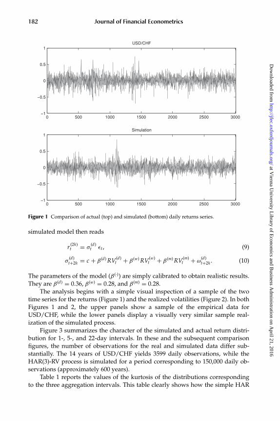
Figure 1 Comparison of actual (top) and simulated (bottom) daily returns series.

simulated model then reads

r (2h)t = σ

(d)t εt , (9)

σ(d)t+2h = c + β (d) RV(d)


t + ω(d)t+2h . (10)

The parameters of the model (β (·)) are simply calibrated to obtain realistic results.They are β (d) = 0.36, β (w) = 0.28, and β (m) = 0.28.

The analysis begins with a simple visual inspection of a sample of the twotime series for the returns (Figure 1) and the realized volatilities (Figure 2). In bothFigures 1 and 2, the upper panels show a sample of the empirical data forUSD/CHF, while the lower panels display a visually very similar sample real-ization of the simulated process.

Figure 3 summarizes the character of the simulated and actual return distri-bution for 1-, 5-, and 22-day intervals. In these and the subsequent comparisonfigures, the number of observations for the real and simulated data differ sub-stantially. The 14 years of USD/CHF yields 3599 daily observations, while theHAR(3)-RV process is simulated for a period corresponding to 150,000 daily ob-servations (approximately 600 years).

Table 1 reports the values of the kurtosis of the distributions correspondingto the three aggregation intervals. This table clearly shows how the simple HAR

at Vienna U


conomics and B

usiness Adm



ownloaded from



0 500 1000 1500 2000 2500 30000

0.1

0.2

0.3

0.4

0.5USD/CHF

0 500 1000 1500 2000 2500 30000

0.1

0.2

0.3

0.4

0.5Simulation

Figure 2 Comparison of actual (top) and simulated (bottom) daily RV series.

−1 −0.8 −0.6 −0.4 −0.2 0 0.2 0.4 0.6 0.8 1 −1 −0.8 −0.6 −0.4 −0.2 0 0.2 0.4 0.6 0.8 1 −1 −0.8 −0.6 −0.4 −0.2 0 0.2 0.4 0.6 0.8 10

0.5

1

1.5

2

2.5

3

3.5

0

2

4

0

0.5

1

1.5

2

2.5

3

Figure 3 Comparison of actual (dotted) and simulated (solid) probability density functions ofreturns for different time horizons. From left to right: daily, weekly, and monthly.

Table 1 Kurtosis.

Daily returns Weekly returns Monthly returns

USD/CHF 4.74 3.82 3.24HAR(3)-RV 4.89 3.90 3.50

Note. Comparison of actual and simulated kurtosis of returns over different time horizons.

at Vienna U


conomics and B

usiness Adm



ownloaded from



0 20 40 60 80 100 120 140−0.1

0

0.1

0.2

0.3

0.4

0.5

0.6

0.7Sample autocorrelation coefficients

k−values

sacf

val

ues

Figure 4 Comparison of actual (dotted) and simulated (solid) autocorrelations of daily realizedvolatility.

model for the realized volatility is able to reproduce not only the excess of kurtosisof the daily returns, but also the empirical cross-over from fat tail to thin taildistributions as the aggregation interval increases.

However, what we are mainly interested in, is the ability of the model toreproduce the volatility persistence of empirical data. Figure 4 shows the actualautocorrelation function of USD/CHF daily realized volatility13 together with theautocorrelation of HAR daily realized volatility simulated over a period corre-sponding to 600 years. This figure shows that the purpose of reproducing thelong memory of the empirical volatility seems to have been fully achieved. It isimportant to remark that theoretically the HAR model for volatility is a short-memory process, which asymptotically should not exhibit hyperbolic decay of theautocorrelation. However, for the aggregation interval considered, the simulatedmodel shows a volatility memory that is at least as long as that of empirical data(and it could even be made much longer, with an appropriate choice of the parame-ters). Also the partial autocorrelation functions share quite a remarkable agreement(Figure 5).

Similar results are also achieved for the distributions of the daily realizedvolatilities (Figure 6) and the scaling behavior of periodograms (Figure 7) whichdisplay a high degree of linearity (typical of true self-similar processes) for bothempirical and simulated data.

13Computed with the two scales estimator of Zhang, Aıt-Sahalia, and Mykland (2005) as described inSection 3.1.

at Vienna U


conomics and B

usiness Adm



ownloaded from



0 5 10 15 20 25 30 35 40 45−0.2

0

0.2

0.4

0.6

0.8

Sample partial autocorrelation coefficientsUSD/CHF

spac

f val

ues

0 5 10 15 20 25 30 35 40 45−0.2

0

0.2

0.4

0.6

0.8Simulated process

spac

f val

ues

Figure 5 Comparison of actual (top) and simulated (bottom) partial autocorrelations of dailyrealized volatility.

−0.1 0 0.1 0.2 0.3 0.4 0.5 0.6−2

0

2

4

6

8

10

12

14RV distributions

Figure 6 Comparison of actual (dotted) and simulated (solid) distributions of daily realizedvolatility.

at Vienna U


conomics and B

usiness Adm



ownloaded from



−12 −11 −10 −9 −8 −7 −6 −5 −4 −3 −210

15

20

25

30

35

log cycles

Simulation

−9 −8 −7 −6 −5 −4 −3 −20

5

10

15

20

log−log PeriodogramUSD/CHF

Figure 7 Comparison of actual (top) and simulated (bottom) periodograms of daily returns onlog–log plane.

3 EMPIRICAL ANALYSIS

3.1 Data

Our data set consists of long tick-by-tick series for USD/CHF, S&P500 Futures,and 30-year US Treasury Bond Futures. The USD/CHF series covers 14 years fromDecember 1989 to December 2003 of tick-by-tick spot log–arithmic middle prices.Log mid prices are computed as averages of the logarithmic bid and ask quotesobtained from the Reuters FXFX screen. In order to avoid explicitly modeling theseasonal behavior of trading activity induced by the weekend, we exclude all therealized volatility taking place from Friday 21:00 GMT to Sunday 22:00 GMT. Forthe S&P500 Futures, we dispose of all transactions from January 1990 to July 2007,while for the T-Bond Futures our data series is from January 1990 to October 2003.

For all three series, we compute daily tick-by-tick realized volatility estimatesemploying the two scales estimator proposed by Zhang, Aıt-Sahalia, and Mykland(2005) with the slower frequency of ten ticks returns. As previously described, thedaily realized volatility is aggregated at weekly and monthly scales according toEquation (4) in order to have comparable realized volatility measures over differenthorizons.

at Vienna U


conomics and B

usiness Adm



ownloaded from



Table 2 HAR(3) estimation.

RV(d)t+1d = c + β(d) RV(d)

t + β(w) RV(w)t + β(m) RV(m)

t + ωt+1d

USD/CHF S&P500 T-Bondc 1.121 0.781 1.494

(5.404) (4.065) (6.475)βd 0.352 0.372 0.039

(13.501) (9.858) (1.672)βw 0.323 0.343 0.412

(7.509) (7.263) (8.941)βm 0.235 0.224 0.361

(6.301) (6.467) (7.987)

Notes. In-sample estimation results of the least squares regression of HAR(3) model for USD/CHFexchange data from December 1989 to December 2003 (3599 daily observations), S&P500 Futures fromJanuary 1990 to July 2007 (4344 observations), and T-Bond Futures from January 1990 to October 2003(3391 observations). Reported in parentheses are the t-statistics based on standard errors computed withNewey–West correction for serial correlation of order 5.

3.2 Estimation

Following the recent literature on realized volatility, we can consider all the termsin Equation (8) as observed and then easily estimate its parameters β (·) by applyingsimple linear regression. Standard OLS regression estimators are consistent andnormally distributed. In order to account for the possible presence of serial corre-lation in the data, the Newey–West covariance correction for serial correlation isemployed.

Table 2 reports the results of the estimation of the HAR-RV model of Equation(8) for three series. From the values of the t-statistics, it is clear that all the threerealized volatilities aggregated over the three different horizons are all highlysignificant. The only exception is the coefficient of daily realized volatility forthe T-Bond. This result may be due to the fact that the time series of the T-Bondrealized volatility seems to show a higher level of noise than that of the S&Pand USD/CHF,14 due to a lower mean tick arrival frequency and a higher impactof market microstructure. The noisier estimation of the daily realized volatilityinduces a lack of significance of the daily volatility component, while weekly andmonthly realized volatilities, being averages over longer periods, arguably containless noise and more information on the volatility process and, hence, receive higherweights from the model.

It is worth noticing that if we accept the interpretation that realized volatilitiesaggregated over different horizons are reasonable proxies for volatilities generatedby the corresponding market components, an interesting by-product of this sim-ple OLS regression is a direct estimate of the market component weights, that is,

14This is confirmed by the comparison of the autocorrelation functions and the much lower R2s of theHAR estimation.

at Vienna U


conomics and B

usiness Adm



ownloaded from



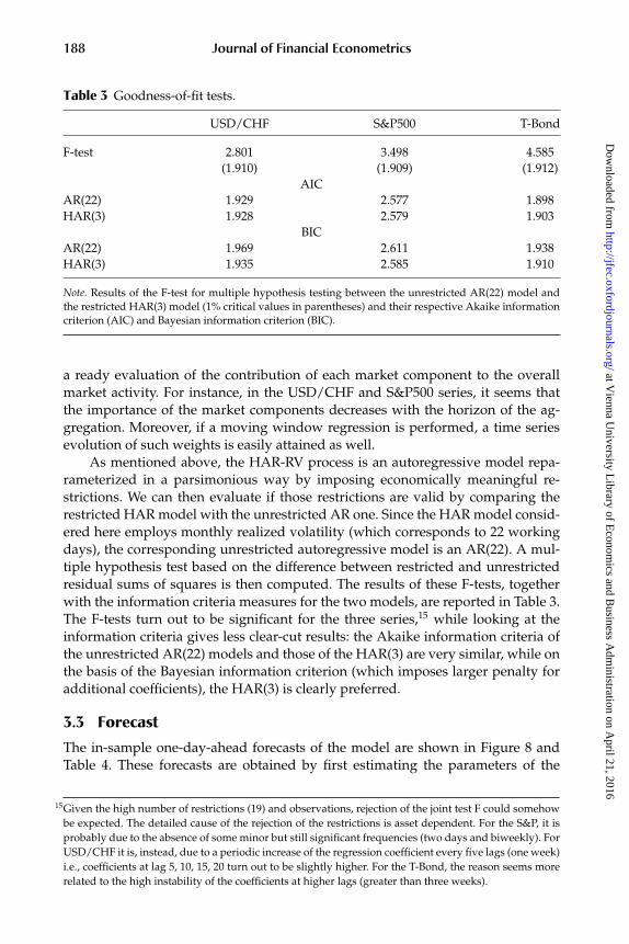
Table 3 Goodness-of-fit tests.

USD/CHF S&P500 T-Bond

F-test 2.801 3.498 4.585(1.910) (1.909) (1.912)

AICAR(22) 1.929 2.577 1.898HAR(3) 1.928 2.579 1.903

BICAR(22) 1.969 2.611 1.938HAR(3) 1.935 2.585 1.910

Note. Results of the F-test for multiple hypothesis testing between the unrestricted AR(22) model andthe restricted HAR(3) model (1% critical values in parentheses) and their respective Akaike informationcriterion (AIC) and Bayesian information criterion (BIC).

a ready evaluation of the contribution of each market component to the overallmarket activity. For instance, in the USD/CHF and S&P500 series, it seems thatthe importance of the market components decreases with the horizon of the ag-gregation. Moreover, if a moving window regression is performed, a time seriesevolution of such weights is easily attained as well.

As mentioned above, the HAR-RV process is an autoregressive model repa-rameterized in a parsimonious way by imposing economically meaningful re-strictions. We can then evaluate if those restrictions are valid by comparing therestricted HAR model with the unrestricted AR one. Since the HAR model consid-ered here employs monthly realized volatility (which corresponds to 22 workingdays), the corresponding unrestricted autoregressive model is an AR(22). A mul-tiple hypothesis test based on the difference between restricted and unrestrictedresidual sums of squares is then computed. The results of these F-tests, togetherwith the information criteria measures for the two models, are reported in Table 3.The F-tests turn out to be significant for the three series,15 while looking at theinformation criteria gives less clear-cut results: the Akaike information criteria ofthe unrestricted AR(22) models and those of the HAR(3) are very similar, while onthe basis of the Bayesian information criterion (which imposes larger penalty foradditional coefficients), the HAR(3) is clearly preferred.

3.3 Forecast

The in-sample one-day-ahead forecasts of the model are shown in Figure 8 andTable 4. These forecasts are obtained by first estimating the parameters of the

15Given the high number of restrictions (19) and observations, rejection of the joint test F could somehowbe expected. The detailed cause of the rejection of the restrictions is asset dependent. For the S&P, it isprobably due to the absence of some minor but still significant frequencies (two days and biweekly). ForUSD/CHF it is, instead, due to a periodic increase of the regression coefficient every five lags (one week)i.e., coefficients at lag 5, 10, 15, 20 turn out to be slightly higher. For the T-Bond, the reason seems morerelated to the high instability of the coefficients at higher lags (greater than three weeks).

at Vienna U


conomics and B

usiness Adm



ownloaded from



Table 4 One-day-ahead in-sample performance.

USD/CHF S&P500 T-Bond

RMSE MAE R2 RMSE MAE R2 RMSE MAE R2

AR(1) 2.803 1.938 0.493 3.927 2.542 0.648 2.770 2.080 0.109AR(3) 2.675 1.830 0.539 3.690 2.364 0.691 2.683 2.010 0.166ARFIMA(5, d, 0) 2.649 1.765 0.559 3.611 2.316 0.703 2.580 1.919 0.237HAR(3) 2.607 1.757 0.565 3.605 2.305 0.707 2.576 1.905 0.236

Notes. Comparison of the in-sample performances of the one-day-ahead forecasts of AR(1), AR(3),ARFIMA(5, d, 0), and HAR(3) models for USD/CHF exchange data, S&P500 Futures, and T-Bond Fu-tures. The parameters of the ARFIMA(5, d, 0) model are estimated with a two-step procedure where thefractional coefficient d is first estimated on the full sample with the GPH algorithm followed by an AR(5)fit. Performance measures are the root mean square error (RMSE), the mean absolute error (MAE), andthe R2 of the Mincer–Zarnowitz regressions.

models on the full sample and then performing a series of static one-step-aheadforecasts. The visual impression of a quite accurate forecast shown in the top andmiddle panels of Figure 8 is confirmed by the remarkably high R2 of the regressionin Table 4. From the right panels of Figure 8, which displays the time series of theforecasting errors, the presence of a significant heteroskedasticity in the residualsis apparent. This remark has led Corsi, Mittnik, Pigorsch, and Pigorsch (2008) toconsider more sophisticated estimation procedures that, being able to take intoaccount this GARCH effect in the volatility residuals, may increase the estimationefficiency of the HAR-RV model.

For comparison purposes other models are added: the AR(1) and AR(3) modelof realized volatility as well as a fractionally integrated model for realized volatilityas employed by Andersen, Bollerslev, Diebold, and Labys (2003). They propose afractional differentiation of the realized volatility series with a fractional coefficientd estimated on the full sample through the GPH algorithm followed by an AR(5)fit. Hence, the model is an ARFIMA(5, d , 0) estimated with a two-step procedure.

In Table 4, the forecasting performances are evaluated on the basis of rootmean square error (RMSE) and mean absolute error (MAE). Moreover, followingthe analysis of Andersen and Bollerslev (1998), Andersen, Bollerslev, and Diebold(2007), and Aıt-Sahalia and Mancini (2008), Table 4 also reports the results of theR2 of the Mincer-Zarnowitz regressions

RV(d)t = b0 + b1Et−1

[(RV

(d)t

)]+ error, (11)

that is, a regression of the ex post realized volatility on a constant and the variousmodel forecasts based on time t − 1 information. In Table 4, the difference inforecasting performance between the standard short-memory models and the onesable to capture the persistence of the empirical data is evident.

Table 5 and Figure 9 report the results for out-of-sample forecasts of the re-alized volatility in which the models are reestimated daily on a moving window

at Vienna U


conomics and B

usiness Adm



ownloaded from



USD/CHF

500 1000 1500 2000 2500 3000 35000

5

10

15

20

25

30

35

40

45actualforecast

500 1000 1500 2000 2500 3000 3500−15

−10

−5

0

5

10

15

20

25

30RESIDUALS

S&P500

500 1000 1500 2000 2500 3000 3500 40000

10

20

30

40

50

60

70actualforecast

500 1000 1500 2000 2500 3000 3500 4000−20

−10

0

10

20

30

40

50RESIDUALS

T-Bond

500 1000 1500 2000 2500 30000

5

10

15

20

25

30actualforecast

0 500 1000 1500 2000 2500 3000−10

−5

0

5

10

15

20RESIDUALS

Figure 8 Comparisons of actual (dotted) and 1-day-ahead in-sample prediction (solid) of the HARmodel for daily realized volatilities (left panels) and the corresponding residuals (right panels).Top: USD/CHF exchange data from December 1989 to July 2003. Middle: S&P500 Futures fromJanuary 1990 to July 2007. Bottom: US Treasury Bond Futures from January 1990 to October 2003.

of 1000 observations. An exception is made for the ARFIMA model for whichthe fractional difference coefficients d are first estimated on the whole sampleand employed to fractionally differentiate the realized volatility series. For thefractional difference operator, we choose the standard cutoff limits of the Taylorexpansion of 1000, which for values of d around 0.4 induces a cutoff error of about4%. After fractional differentiation, the optimal length of the moving windowused in the estimation of the AR parameters turns out to be about 250 days. The

at Vienna U


conomics and B

usiness Adm



ownloaded from



Table 5 Out-of-sample forecasts.

1 day 1 week 2 weeks

RMSE MAE R2 RMSE MAE R2 RMSE MAE R2

USD/CHFAR(1) 2.540 1.796 0.497 2.699 2.089 0.213 2.764 2.178 0.038AR(3) 2.459 1.699 0.530 2.194 1.673 0.523 2.406 1.909 0.316ARFIMA 2.430 1.674 0.546 1.864 1.362 0.611 1.812 1.360 0.576HAR(3) 2.377 1.622 0.551 1.878 1.361 0.609 1.829 1.381 0.570

S&P500AR(1) 4.170 2.669 0.640 4.878 3.550 0.323 5.273 4.012 0.166AR(3) 3.953 2.518 0.680 3.783 2.583 0.613 4.381 3.184 0.408ARFIMA 4.085 2.762 0.651 3.409 2.403 0.678 3.502 2.478 0.633HAR(3) 3.873 2.475 0.696 3.352 2.237 0.698 3.539 2.437 0.627

T-BondAR(1) 2.746 2.044 0.152 1.971 1.505 0.076 1.797 1.388 0.075AR(3) 2.672 1.984 0.197 1.820 1.396 0.246 2.406 1.909 0.316ARFIMA 2.587 1.914 0.256 1.505 1.140 0.442 1.371 1.024 0.445HAR(3) 2.568 1.886 0.264 1.516 1.153 0.440 1.401 1.052 0.438

Notes. Comparison of the out-of-sample performances of the 1-day-, 1-week-, and 2-week-ahead forecastsof the AR(1), AR(3), ARFIMA(5, d, 0), and HAR(3) models for USD/CHF exchange data, S&P500 Futures,and T-Bond Futures. The AR(1), AR(3), and HAR(3) are daily reestimated on a moving window of 1000observations. For the ARFIMA(5, d, 0), the coefficient of fractional integration d is preestimated on thewhole sample. After fraction differentiation with a cutoff limit of the Taylor expansion of 1000, theoptimal length of the moving window for the estimation of the AR(5) parameters is around 250 days.Performance measures are the root mean square error (RMSE), the mean absolute error (MAE), and theR2 of the Mincer–Zarnowitz regressions. The multistep-ahead forecasts are evaluated comparing theaggregated realized and predicted volatility over the multiperiod horizon.

forecasting performances are compared over three different time horizons: oneday, one week, and two weeks. The multistep-ahead forecasts are evaluated con-sidering the aggregated volatility realized and predicted over the multiperiodhorizon. For an h-step-ahead forecast, the target function is then

∑hj=0 RV(d)

t+ j andthe Mincer–Zarnowitz regression becomes

h∑j=0

RV(d)t+ j = b0 + b1Et−h

⎡⎣ h∑

j=0

RV(d)t+ j

⎤⎦ + error. (12)

Out-of-sample, it turns out that the parsimonious HAR(3) model steadily out-performs the short-memory models at all the three time horizons considered (oneday, one week, and two weeks) and compares similarly to the true long-memoryARFIMA model. It is noteworthy that though the superior performance of theARFIMA and HAR(3) was already apparent at daily horizon, it becomes strikingat weekly and biweekly horizons. The reason is that the AR(1) and AR(3) models

at Vienna U


conomics and B

usiness Adm



ownloaded from



USD/CHFAR(3)

1500 2000 2500 3000 350068

1012141618202224

actualforecast

1500 2000 2500 3000 350068

1012141618202224

1500 2000 2500 3000 350068

1012141618202224

S&P500

1500 2000 2500 3000 3500 40005

10

15

20

25

30

35

40

45

1500 2000 2500 3000 3500 400005

1015202530354045

1500 2000 2500 3000 3500 40005

10

15

20

25

30

35

40

45

T-Bond

1500 2000 2500 3000 35004

6

8

10

12

14

16

18

1500 2000 2500 3000 35004

6

8

10

12

14

16

18

1500 2000 2500 3000 35004

6

8

10

12

14

16

18

ARFIMA(5,d,0) HAR(3)

AR(3) ARFIMA(5,d,0) HAR(3)

AR(3) ARFIMA(5,d,0) HAR(3)

actualforecast

actualforecast

actualforecast

actualforecast

actualforecast

actualforecast

actualforecast

actualforecast

Figure 9 Comparison of the out-of-sample performances of 2-week-ahead forecasts of the AR(3),ARFIMA(5, d, 0), and HAR(3) models for USD/CHF exchange data (top), S&P500 Futures (mid-dle), and T-Bond Futures (bottom). The continuous line is the aggregated prediction, while thedotted line is the ex post aggregated realized volatility over a 2-week period. The AR(3) and HAR(3)are daily reestimated on a moving window of 1000 observations. For the ARFIMA(5, d, 0), the frac-tional difference parameter d is preestimated on the whole sample. After fraction differentiationwith a cutoff limit of 1000, the optimal length of the moving window for the estimation of theAR(5) parameters is around 250 days.

have a memory which is too short compared to the forecasting horizon and henceconverge too quickly to their unconditional mean for longer forecasting horizons.

This explanation is confirmed by Figure 9 which compares the dynamic be-havior of the different models for the two-week forecasting periods. For this timehorizon, the importance of long memory becomes manifest. What is surprising isthe ability of the HAR-RV model to attain these results with only a few parameters.

Confronting the results of the HAR(3) and ARFIMA(5,d ,0), Table 5 shows thatthe performances of the two models are comparable (with a slight advantage for theHAR model for daily and weekly horizons and for the ARFIMA for the biweekly

at Vienna U


conomics and B

usiness Adm



ownloaded from



horizon).16 However, it should be noted that while the HAR model is extremelysimple and straightforward to implement (even on a daily moving window), theARFIMA model is much more cumbersome and complicated (especially on movingwindows). Moreover, ARFIMA model estimation and forecasts are quite sensitiveto the choice of the Taylor expansion cutoff limit of the fractional difference operatorand, for the GPH estimation of d , also quite sensitive to the choice of the frequencycut off.

4 CONCLUSIONS

We propose a volatility model in which an additive volatility cascade inspired bythe Heterogeneous Market Hypothesis leads to a simple AR-type model in therealized volatility. This model has the feature of considering volatilities realizedover different interval sizes. We term this model HAR-RV. The new HAR-RV modelseems to successfully achieve the purpose of modeling the long-memory behaviorof volatility in a very simple and parsimonious way (although not formally be-longing to the class of long-memory models). Moreover, in spite of the simplicityof its structure and estimation, the HAR-RV model shows remarkably good fore-casting performance. Based on the out-of-sample forecasting results for the threelong series of realized volatilities of USD/CHF, S&P500, and T-Bond, the HAR(3)model steadily outperforms the short-memory models at all the time horizons con-sidered (one day, one week, and two weeks) and is comparable to the much morecomplicated and tedious to estimate long-memory ARFIMA model.

The simplicity of the proposed model allows it to be easily extended in vari-ous directions. Other statistically and economically significant variables could besimply added as additional regressors. For example, different measures of jumpscould be included (after separating them from the continuous volatility compo-nents) as in Andersen et al. (2007) and Corsi, Pirino, and Reno (2008). Leverageeffects can be considered by simply adding lagged positive and negative returnsas regressors (see Corsi and Reno 2008). Extensions of the HAR model to accountfor nonlinear effects can be obtained by combining it with smooth transition ortree-structured models as in McAleer and Medeiros (2008) and Audrino and Corsi(2008), respectively. The same logic based on heterogeneous components can beapplied to other different models such as the alternative approach to modelingand forecasting realized volatility proposed in the Multiplicative Error Modelsof Engle and Gallo (2006). Moreover, its simple autoregressive structure suggestsa natural way to extend it to the multivariate case by developing a Vector-HARmodel analogous to the standard VAR model as in Bauer and Vorkink (2007).

Received July 7, 2008; revised December 31, 2008; accepted January 14, 2009.

16It should be recalled, however, that the ARFIMA forecasts are not truly out of sample, since the fractionaldifference coefficient d is estimated on the whole sample.

at Vienna U


conomics and B

usiness Adm



ownloaded from



REFERENCES

Aıt-Sahalia, Y., and L. Mancini. 2008. “Out of sample forecasts of quadratic variation.”Journal of Econometrics 147: 17–33.

Alfarano, S., and T. Lux. 2007. “A noise trader model as a generator of apparent financialpower laws and long memory.” Macroeconomic Dynamics 11: 80–101.

Andersen, T. G., and T. Bollerslev. 1997. “Heterogeneous information arrivals and returnvolatility dynamics: Uncovering the long run in high frequency data.” Journal ofFinance 52: 975–1005.

Andersen, T. G., and T. Bollerslev. 1998. “Answering the skeptics: Yes, standard volatilitymodels do provide accurate forecasts.” International Economic Review 39: 885–905.

Andersen, T. G., T. Bollerslev, and F. X. Diebold. 2007. “Roughing it up: Including jumpcomponents in the measurement, modeling, and forecasting of return volatility.”The Review of Economic and Statistics 89(4), 701–720.

Andersen, T. G., T. Bollerslev, F. X. Diebold, and H. Ebens. 2001. “The distribution ofstock returns volatilities.” Journal of Financial Economics 61: 43–76.

Andersen, T. G., T. Bollerslev, F. X. Diebold, and P. Labys. 2001. “The distribution ofrealized exchange rate volatility.” Journal of the American Statistical Association 96:42–55.

Andersen, T. G., T. Bollerslev, F. X. Diebold, and P. Labys. 2003. “Modeling and fore-casting realized volatility.” Econometrica 71: 579–625.

Arneodo, A., J. Muzy, and D. Sornette. 1998. “Causal cascade in stock market from the‘infrared’ to the ‘ultraviolet’.” European Physical Journal, B 2: 277–282.

Audrino, F., and F. Corsi. 2008. “Modeling tick-by-tick realized correlations.” Universityof St. Gallen, Department of Economics, Discussion paper No. 2008-05.

Barndorff-Nielsen, O., and N. Shephard. 2002a. “Econometric analysis of realizedvolatility and its use in estimating stochastic volatility models.” Journal of the RoyalStatistical Society, B 64: 253–280.

Barndorff-Nielsen, O., and N. Shephard. 2002b. “Estimating quadratic variation usingrealized variance.” Journal of Applied Econometrics 17: 457–477.

Bauer, G., and K. Vorkink. 2007. “Multivariate realized stock market volatility.” Workingpaper, Bank of Canada.

Breymann, W., S. Ghashghaie, and P. Talkner. 2000. “A stochastic cascade modelfor FX dynamics.” International Journal of Theoretical and Applied Finance 3: 357–360.

Calvet, L., and A. Fisher. 2004. “How to forecast long-run volatility: Regime switchingand the estimation of multifractal processes.” Journal of Financial Econometrics 2:49–83.

Calvet, L., and A. Fisher. 2007. “Multifrequency news and stock returns.” Journal ofFinancial Economics 86: 178–212.

Comte, F., and E. Renault. 1998. “Long memory in continuous time stochastic volatilitymodels.” Mathematical Finance 8: 291–323.

Corsi, F., S. Mittnik, C. Pigorsch, and U. Pigorsch. 2008. “The volatility of realizedvolatility.” Econometric Reviews 27: 46–78.

Corsi, F., D. Pirino, and R. Reno. 2008. “Volatility forecasting: The jumps do matter.”Working paper, University of Siena.

at Vienna U


conomics and B

usiness Adm



ownloaded from



Corsi, F., and R. Reno. 2008. “Volatility components: Heterogeneity, leverage, andjumps.” Working paper, University of Siena.

Dacorogna, M., U. Muller, R. Dav, R. Olsen, and O. Pictet. 1998. “Modelling short-term volatility with GARCH and HARCH models.” In Nonlinear Modelling of HighFrequency Financial Time Series, ed. C. Dunis and B. Zhou, 161–76. Chichester, UK:Wiley.

Dacorogna, M. M., R. Genay, U. A. Muller, R. B. Olsen, and O. V. Pictet. 2001. AnIntroduction to High-Frequency Finance. San Diego, CA: Academic Press.

Ding, Z., C. Granger, and R. Engle. 1993. “A long memory property of stock marketreturns and a new model.” Journal of Empirical Finance 1: 83–106.

Engle, R., and G. Gallo. 2006. “A multiple indicators model for volatility using intra-daily data.” Journal of Econometrics 131: 3–27.

Forsberg, L., and E. Ghysels. 2007. “Why do absolute returns predict volatility so well?”Journal of Financial Econometrics 5: 31–67.

Gencay, R., and F. Selcuk. (2004). “Asymmetry of information flow between volatilitiesacross time scales.” North American Winter Meetings 90, Econometric Society.

Ghashghaie, S., W. Breymann, J. Peinke, P. Talkner, and Y. Dodge. 1996. “Turbulentcascades in foreign exchange markets.” Nature 381: 767–770.

Ghysels, E., P. Santa-Clara, and R. Valkanov. 2006. “Predicting volatility: Getting themost out of return data sampled at different frequencies.” Journal of Economet-rics 131: 59–95.

Ghysels, E., A. Sinko, and R. Valkanov. 2006. “Midas regressions: Further results andnew directions.” Econometric Reviews 26: 53–90.

Granger, C. 1980. “Long memory relationships and the aggregation of dynamic mod-els.” Journal of Econometrics 14: 227–238.

LeBaron, B. 2001. “Stochastic volatility as a simple generator of financial power lawsand long memory.” Quantitative Finance 1: 621–631.

LeBaron, B. 2006. “Agent-based financial markets: Matching stylized facts with style.”In Post Walrasian Macroeconomics: Beyond the DSGE Model, ed. D. Colander, 221–235.Cambridge, UK: Cambridge University Press.

Lobato, I., and N. Savin. 1998. “Real and spurious long-memory properties of stockmarket data.” Journal of Business and Economic Statistics 16: 261–283.

Lux, T., and M. Marchesi. 1999. “Scaling and criticality in a stochastic multi-agent modelof financial market.” Nature 397: 498–500.

Lynch, P., and G. Zumbach. 2003. “Market heterogeneities and the causal structure ofvolatility.” Quantitative Finance 3: 320–331.

McAleer, M., and M. Medeiros. 2008. “A multiple regime smooth transition heteroge-neous autoregressive model for long memory and asymmetries.” Journal of Econo-metrics 147: 104–119.

Muller, U., M. Dacorogna, R. Dav, R. Olsen, O. Pictet, and J. von Weizsacker. 1997.“Volatilities of different time resolutions – Analysing the dynamics of market com-ponents.” Journal of Empirical Finance 4: 213–239.

Muller, U., M. Dacorogna, R. Dav, O. Pictet, R. Olsen, and J. Ward. 1993. “Fractals and in-trinsic time – A challenge to econometricians.” 39th International AEA Conferenceon Real Time Econometrics, 14–15 October 1993, Luxembourg.

Peters, E. 1994. Fractal Market Analysis. New York: Wiley.

at Vienna U


conomics and B

usiness Adm



ownloaded from



Rossi, A., and G. Gallo. 2006. “Volatility estimation via hidden Markov models.” Journalof Empirical Finance 13: 203–230.

Zhang, L., Y. Aıt-Sahalia, and P. A. Mykland. 2005. “A tale of two time scales: Determin-ing integrated volatility with noisy high frequency data.” Journal of the AmericanStatistical Association 100: 1394–1411.

at Vienna U


conomics and B

usiness Adm



ownloaded from


a simple approximate long-memory model of realized...

Documents