a) simplified b) with classical and stl decomposition
TRANSCRIPT

1
Time series: forecasting methods
a) simplified
b) with classical and STL decomposition
Agostino Nuzzolo ([email protected])
Antonio Comi ([email protected])

Bibliography
2
Forecasting: principles and practiceby Rob J Hyndman (Author), George Athanasopoulos (Author)
https://www.otexts.org/book/fpp

Time series forecasting
Given the values y1,…,yT of variable yobserved until time T
Let
time T forecast of future value after hfuture realizations
3
T h/Ty

Forecasting methods: classification
• Simple forecast methods
• Methods with Classical and STL decomposition
• Methods with exponential smoothing
• ARIMA models (not considered)
• Regressions
Multiple regressions.
Artificial Neural Network models
4

Some simple forecasting methods
• Naive method
• Seasonal naive method
• Average method
• Average seasonal method
• Drift method
5

Some simple forecasting methodsNaive method
All forecasts T+h are simply set to be the value of the last
observation yT.
This method can give good results if:
- trend, cycle and seasonality are limited,
- residuals not too much variable.
6

Some simple forecasting methodsSeasonal naive method
A method similar to naïve is useful for highly seasonal data.
In this case, we set each forecast to be equal to the last observed
value from the same season (e.g., the same hour of the previous
day). Formally, the forecast for time T+h is equal to
This method can be used when seasonality is quite constant
7
where = seasonal periopd, = 1 1T h kmy m k h m
Integer part

Some simple forecasting methodsExample – Seasonal naive forecast for one week (5 days
per week)
830-minute interval (week)
Every forecasted day is equal to the same day of previous week

Some simple forecasting methodsAverage method
The forecasts of all future values T+h are equal to the mean of the
historical data y1,…,yT
This method can give good results:
- if trend, cycle and seasonality are limited,
- residuals are very variable.
9
1 2T h/ T Ty y y y ... y T

Some simple forecasting methodsSeasonal average method
A method similar to average method is useful for highly seasonal
data.
In this case, we set each forecast to be equal to the average of the
observed values of the same season (e.g., the same hour of the
previous days).
10

Some simple forecasting methodsDrift methodA variation on the naïve method is to allow the forecasts to increase
or decrease over time, where the amount of change over time
(called the drift) is set to be the average change seen in the
historical data.
So the forecast for time T+h is given by:
This is equivalent to drawing a line between the first and last
observation, and extrapolating it into the future.
This method can be used when trend is the very prevalent
component.
11
11
21 1
TT
T t t T
t
y yhy y y y h
T T

Some simple forecasting methods
• Naive method: limited weight of trend, cycle and seasonality and
with residual not scattered
• Seasonal naive method: seasonality is predominant with
constant values among the seasons
• Average method: limited weight of trend, cycle and seasonality
and with residual scattered
• Average seasonal method: seasonality is prevalent, with
variability among seasons
• Drift method: trend is predominant
12

Forecasting methods: classification
• Simple forecast methods
• Methods with Classical and STL decomposition
• Methods with exponential smoothing
• ARIMA models
• Neural Network models
13
.
We separately forecast:
- the seasonal component of
- the trend/cyclic component of .
The forecasted seasonal component is assumed equal to the
seasonal component of the training period.
The forecasted trend/cyclic component is assumed equal the
decomposed trend/cycle value of the last available observation.
14
Forecasting with decomposition
tS
tT
T h/Ty
T h/Ty

15
Forecasting with classical decompositionExample – classical decomposition
Travel time line 343 from Ponte Mammolo to Conca d’Oro
Travel time to
be forecasted

Example of forecasting with classical decomposition
The time series includes 8 successive periods “ Monday – Friday”
of Bus travel time in 30 minute intervals of line 343 ( see following
slides).
We want forecast values between 14:15 of Wednesday and 22:45
of Friday in the last period and compare them with observed data.
To forecast the decomposed time series, we separately forecast
the seasonal component, , and the trend/cyclic component
.
The forecasted seasonal component is assumed equal to the
seasonal component of last Monday-Friday period.
The forecasted trend/cyclic component is assumed equal the
decomposed value of 14:15 of Wednesday
16
Forecasting with classical decomposition
tS
tT

17
Forecasting with classical decompositionExample: forecasted and observed values
time interval trend componentseasonal
componentforecasts data observed
1171 2515,7 -49,6 2415,0 2802,0
1172 2515,7 31,5 2496,6 2589,0
1173 2515,7 62,6 2529,0 2446,0
1174 2515,7 271,2 2738,0 2549,0
1175 2515,7 482,9 2954,2 2643,0
1176 2515,7 550,4 3028,7 2612,0
1177 2515,7 592,6 3075,0 2572,0
1178 2515,7 725,0 3212,3 2551,0
1179 2515,7 532,0 3024,8 2433,0
1180 2515,7 415,1 2911,8 2552,0
1181 2515,7 281,8 2781,0 2453,0
1182 2515,7 -45,4 2454,9 2257,0
1183 2515,7 -434,0 2066,7 1845,0
1184 2515,7 -559,1 1941,5 1843,0
1185 2515,7 -656,5 1671,4 1730,0
1186 2515,7 -738,6 1587,8 1617,0
1187 2515,7 -797,7 1528,7 1575,0
1188 2515,7 -858,8 1467,6 1531,0
1189 2515,7 -938,4 1388,6 1712,0
1190 2515,7 -846,3 1482,5 1696,0
1191 2515,7 -483,5 1848,0 1905,0
1192 2515,7 -183,8 2150,5 2272,0
18
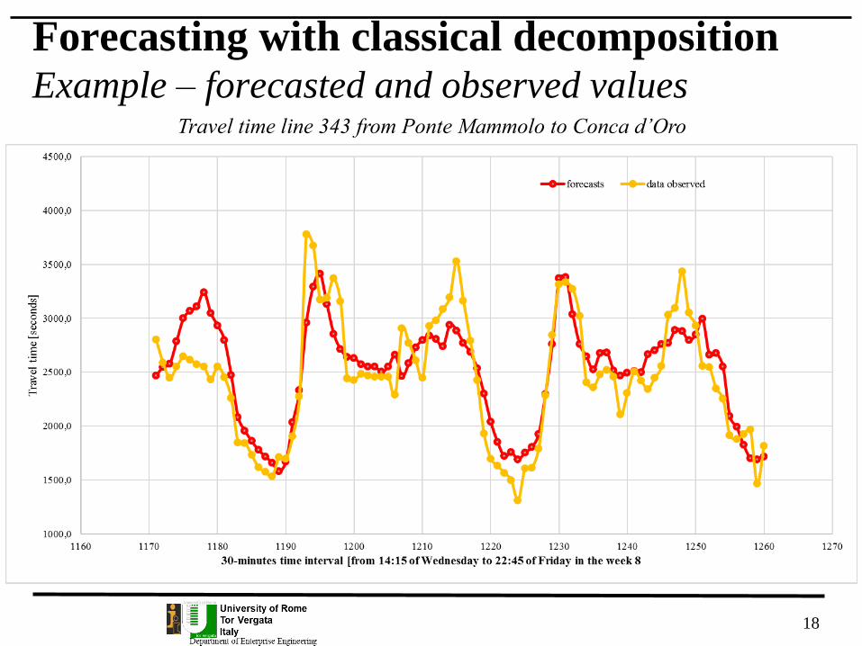
Forecasting with classical decompositionExample – forecasted and observed values
Travel time line 343 from Ponte Mammolo to Conca d’Oro

• Forecast accuracy measures
• Training and test sets
• Cross-validation (not dealt)
19
Evaluation of forecast accuracy
When choosing models, it is common to use a portion of the
available data for fitting, and use the rest of the data for testing
the model. Then the testing data can be used to measure how well
the model is likely to forecast on new data.
The size of the test set is typically about 20% of the total sample,
although this value depends on how long the sample is and how far
ahead you want to forecast.
The size of the test set should ideally be at least as large as the
maximum forecast horizon required.
20
Evaluation forecast accuracyTraining set and test set

Let yi denote the i-th observation and denote a forecast of yi.
Scale-dependent errors• The forecast error is simply
which is on the same scale as the data.
Accuracy measures that are based on ei are therefore scale-
dependent and cannot be used to make comparisons between
series that are on different scales.
21
Evaluation forecast accuracy 1Forecast accuracy measures
iy
i i iˆe y y

The two most commonly used scale-dependent measures are based on
the absolute errors or squared errors :
When comparing forecast methods on a single data set, the MAE
is popular as it is easy to understand and compute.
22
Evaluation forecast accuracy 2Forecast accuracy measures
2
Mean absolute error: MAE = mean
Root mean squared error: RMSE= mean
i
i
e
e
ie 2
ie

• Percentage errors. The percentage error is given by
Percentage errors have the advantage of being scale-independent, and so are
frequently used to compare forecast performance between different data sets.
The most commonly used measure is:
Measures based on percentage errors have the disadvantage of
being infinite or undefined if yi=0 for any i in the period of
interest, and having extreme values when any yi is close to zero.
Another problem with percentage errors that is often overlooked is that they assume a
meaningful zero. For example, a percentage error makes no sense when measuring the
accuracy of temperature forecasts on the Fahrenheit or Celsius scales
23
Evaluation forecast accuracy 3Forecast accuracy measures
100i i ip e y
Mean absolute percentage error: MAPE = mean ip

Evaluation forecast accuracy
Example: forecast errors
24
time interval
of the day of
analysis
forecasted
trend
component
Forecasted
seasonal
component
TOTAL
Forecasts
data
observedei ABS(ei) e2
i pi ABS(pi)
1171 2515,7 -49,6 2466,1 2802,0 335,9 335,9 112798,6 12% 12%
1172 2515,7 31,5 2547,2 2589,0 41,8 41,8 1747,5 2% 2%
1173 2515,7 62,6 2578,4 2446,0 -132,4 132,4 17518,6 -5% 5%
1174 2515,7 271,2 2786,9 2549,0 -237,9 237,9 56611,4 -9% 9%
1175 2515,7 482,9 2998,7 2643,0 -355,7 355,7 126514,3 -13% 13%
1176 2515,7 550,4 3066,2 2612,0 -454,2 454,2 206283,4 -17% 17%
1177 2515,7 592,6 3108,4 2572,0 -536,4 536,4 287686,3 -21% 21%
1178 2515,7 725,0 3240,7 2551,0 -689,7 689,7 475732,2 -27% 27%
1179 2515,7 532,0 3047,8 2433,0 -614,8 614,8 377953,0 -25% 25%
1180 2515,7 415,1 2930,8 2552,0 -378,8 378,8 143493,7 -15% 15%
1181 2515,7 281,8 2797,5 2453,0 -344,5 344,5 118703,0 -14% 14%
1182 2515,7 -45,4 2470,4 2257,0 -213,4 213,4 45521,6 -9% 9%
1183 2515,7 -434,0 2081,7 1845,0 -236,7 236,7 56035,9 -13% 13%
1184 2515,7 -559,1 1956,6 1843,0 -113,6 113,6 12911,2 -6% 6%
1185 2515,7 -656,5 1859,3 1730,0 -129,3 129,3 16709,1 -7% 7%
1186 2515,7 -738,6 1777,2 1617,0 -160,2 160,2 25656,4 -10% 10%
1187 2515,7 -797,7 1718,0 1575,0 -143,0 143,0 20455,1 -9% 9%
1188 2515,7 -858,8 1656,9 1531,0 -125,9 125,9 15859,7 -8% 8%
1189 2515,7 -938,4 1577,3 1712,0 134,7 134,7 18143,7 8% 8%
1190 2515,7 -846,3 1669,4 1696,0 26,6 26,6 706,6 2% 2%
1191 2515,7 -483,5 2032,3 1905,0 -127,3 127,3 16200,8 -7% 7%
1192 2515,7 -183,8 2332,0 2272,0 -60,0 60,0 3598,0 -3% 3%
MAESec
234,4
RMSE 284,8
MAPE 10%
Travel time line 343 from Ponte Mammolo to Conca d’Oro

Not dealt
25
Evaluation forecast accuracyCross-validation

A residual or error in forecasting is the difference between an
observed value and its forecast based on other observations:
For time series forecasting, a residual is based on one-step
forecasts; that is is the forecast of yt based on observations
y1,…,yt−1.
26
Residual diagnostics [1/5]
i i iˆe y y
iy

A good forecasting method will yield residuals with the following
properties:
• the residuals are uncorrelated. If there are correlations between
residuals, then there is information left in the residuals which
should be used in computing forecasts.
• the residuals have zero mean. If the residuals have a mean
other than zero, then the forecasts are biased.
27
Residual diagnostics [2/5]

Any forecasting method that does not satisfy these properties can
be improved.
That does not mean that forecasting methods that satisfy these
properties can not be improved.
It is possible to have several forecasting methods for the same data
set, all of which satisfy these properties. Checking these properties
is important to see if a method is using all available information
well, but it is not a good way for selecting a forecasting method.
28
Residual diagnostics [3/5]

If either of these two properties is not satisfied, then the forecasting
method can be modified to give better forecasts.
Adjusting for bias is easy: if the residuals have mean m, then simply
add m to all forecasts and the bias problem is solved.
Fixing the correlation problem is harder and it is not addressed here.
In addition to these essential properties, it is useful (but not
necessary) for the residuals to also have the following two properties.
• The residuals have constant variance.
• The residuals are normally distributed.
These two properties make the calculation of prediction intervals
easier (see the next section for an example).
29
Residual diagnostics [4/5]

Prediction intervals
It gives an interval within which we expect yi to lie with a
specified probability. For example, assuming the forecast errors
are uncorrelated and normally distributed, then a simple 95%
prediction interval for the next observation in a time series is
where is an estimate of the standard deviation of the forecast
distribution. In forecasting, it is common to calculate 80% intervals
and 95% intervals, although any percentage may be used.
In the previous example, the prediction intervals are equal to
+/- 545,1 sec., but consider that the errors are correlated.
30
1 96iˆ ˆy .

However, a forecasting method that does not satisfy these properties
cannot necessarily be improved.
Sometimes applying a transformation such as a logarithm or a square
root may assist with these properties, but otherwise there is usually
little you can do to ensure your residuals have constant variance and
have a normal distribution. Instead, an alternative approach to
finding prediction intervals is necessary.
31
Residual diagnostics [5/5]

Residual diagnosticsExample of residual diagnostic for previous
forecast
32
Average ei
-61.1 278.1
rk 1 2 3 4
0.80 0.55 0.23 0.15

Residual diagnosticsExample of residual diagnostic for previous
forecast
• In this example, residuals have error bias = - 61.1
seconds and they are strongly correlated
• Therefore, potentially a better forecasting method
could be found
33

Forecasting with STL decompositionExample
stl.TV=stl(ts.TV, t.window=360, s.window="periodic",
robust=TRUE)
34
Travel time to
be forecasted:
week 9

35
Forecasting with STL decompositionExample: forecasted and observed values
time interval trend componentseasonal
componentforecasts data observed
1171 2414,9 32,7 2447,6 2802,0
1172 2414,9 74,0 2488,9 2589,0
1173 2414,9 97,3 2512,2 2446,0
1174 2414,9 257,1 2671,9 2549,0
1175 2414,9 387,1 2801,9 2643,0
1176 2414,9 405,2 2820,1 2612,0
1177 2414,9 197,4 2612,3 2572,0
1178 2414,9 310,8 2725,6 2551,0
1179 2414,9 203,0 2617,9 2433,0
1180 2414,9 275,0 2689,9 2552,0
1181 2414,9 193,1 2608,0 2453,0
1182 2414,9 -48,4 2366,5 2257,0
1183 2414,9 -431,3 1983,5 1845,0
1184 2414,9 -541,7 1873,2 1843,0
1185 2414,9 -641,4 1773,4 1730,0
1186 2414,9 -728,1 1686,8 1617,0
1187 2414,9 -784,5 1630,4 1575,0
1188 2414,9 -842,8 1572,1 1531,0
1189 2414,9 -887,4 1527,4 1712,0
1190 2414,9 -804,1 1610,7 1696,0
1191 2414,9 -470,1 1944,8 1905,0
1192 2414,9 -153,5 2261,3 2272,0

36
Forecasting with STL decompositionExample – forecasted and observed values
Travel time line 343 from Ponte Mammolo to Conca d’Oro
1000.0
1500.0
2000.0
2500.0
3000.0
3500.0
4000.0
4500.0
1160 1170 1180 1190 1200 1210 1220 1230 1240 1250 1260 1270
Tra
vel
tim
e [s
eco
nd
s]
30-minutes time interval [from 14:15 of Wednesday to 22:45 of Friday in the week 8
forecasts data observed

Residual diagnosticsExample of error diagnostic for forecasting with
STL decomp.
37
Average ei S
-31.7 222.7
rk 1 2 3 4
0.79 0.39 0.07 0.01
-400.0
-200.0
0.0
200.0
400.0
600.0
800.0
1000.0
1200.0
1170 1180 1190 1200 1210 1220 1230 1240 1250 1260 1270
seco
nd
s
30-minutes time interval
residuals
MAE 164,9
RMSE 225,0
MAPE 7%

Comparison Classical – STL forecasting
Classical
38
STL
Average ei S
-31.7 222.7
Average ei
-61.1 278.1
MAE 164.9
RMSE 225.0
MAPE 7%
MAE 234.4
RMSE 284.8
MAPE 10%
The basic steps in a forecasting task
A forecasting task usually involves five basic steps.
Step 1: Problem definition.
Step 2: Gathering information.
Step 3: Preliminary (exploratory) analysis.
Step 4: Choosing and fitting models.
Step 5: Using and evaluating a forecasting model.
39

The basic steps in a forecasting taskStep 1: Problem definition
Often this is the most difficult part of forecasting. Defining the
problem carefully requires an understanding of the way the
forecasts will be used, who requires the forecasts, and how the
forecasting function fits within the organization requiring the
forecasts.
A forecaster needs to spend time talking to everyone who will be
involved in collecting data, maintaining databases, and using the
forecasts for future planning.
40

The basic steps in a forecasting taskStep 2: Gathering information
There are always at least two kinds of information required:
(a) statistical data, and
(b) the accumulated expertise of the people who collect the data
and use the forecasts.
Often, it will be difficult to obtain enough historical data to be able
to fit a good statistical model. However, occasionally, very old data
will be less useful due to changes in the system being forecast.
41

The basic steps in a forecasting taskStep 3: Preliminary (exploratory) analysis
Always start by graphing the data.
Are there consistent patterns?
Is there a significant trend?
Is seasonality important?
Is there evidence of the presence of cycles?
Are there any outliers in the data that need to be explained by those
with expert knowledge?
How strong are the relationships among the variables available
for analysis?
42

The basic steps in a forecasting taskStep 4: Choosing and fitting models
The best model to use depends on the availability of historical data,
the strength of relationships between the forecast variable and any
explanatory variables, and the way the forecasts are to be used.
It is common to compare two or three potential models.
Each model is itself an artificial construct that is based on a set of
assumptions (explicit and implicit) and usually involves one or
more parameters which must be "fitted" using the known historical
data.
43

The basic steps in a forecasting taskStep 5: Using and evaluating a forecasting model
Once a model has been selected and its parameters estimated, the
model is used to make forecasts.
The performance of the model can only be properly evaluated after
the data for the forecast period have become available.
A number of methods have been developed to help in assessing the
accuracy of forecasts.
There are also organizational issues in using and acting on the
forecasts.
44

Forecast method to use
• The choice of forecast method depends on:
Forecast horizon:
Among few time intervals h (e.g. for the next 10-slots of the next hour)
Among few time intervals h (e.g. for the next 10-slots of the next
hours)
Among different time intervals h (es. intervals of 10 minutes of
tomorrow)
Among many time intervals h (es. Intervals of 10 minutes of a day of
next month or year)
Weight of the time series components:
Trend
Cycle
Seasonality
Residual
45

APPENDIX A
Other forecast accuracy measures
46

They also have the disadvantage that they put a heavier penalty on
negative errors than on positive errors. This observation led to the
use of the so-called "symmetric" MAPE (sMAPE). It is defined by
However, if yi is close to zero, is also likely to be close to zero.
Thus, the measure still involves division by a number close to zero,
making the calculation unstable. Also, the value of sMAPE can be
negative, so it is not really a measure of “absolute percentage
errors” at all.
47
Evaluation forecast accuracyForecast accuracy measures
sMAPE = mean 200 i i i iˆ ˆy y y y
iy

• Scaled errors
Scaled errors were proposed as an alternative to using percentage errors
when comparing forecast accuracy across series on different scales.
They proposed scaling the errors based on the training MAE from a
simple forecast method. For a non-seasonal time series, a useful way to
define a scaled error uses naïve forecasts:
48
Evaluation forecast accuracy [1/4]Forecast accuracy measures
1
2
1
1
j
j T
t t
t
eq
y yT

Because the numerator and denominator both involve values on the
scale of the original data, qj is independent of the scale of the data.
A scaled error is less than one if it arises from a better forecast than
the average naïve forecast computed on the training data.
Conversely, it is greater than one if the forecast is worse than the
average naïve forecast computed on the training data.
For seasonal time series, a scaled error can be defined using
seasonal naïve forecasts:
49
Forecast accuracy measures [2/4]Scaled errors
1
1
j
j T
t t m
t m
eq
y yT m
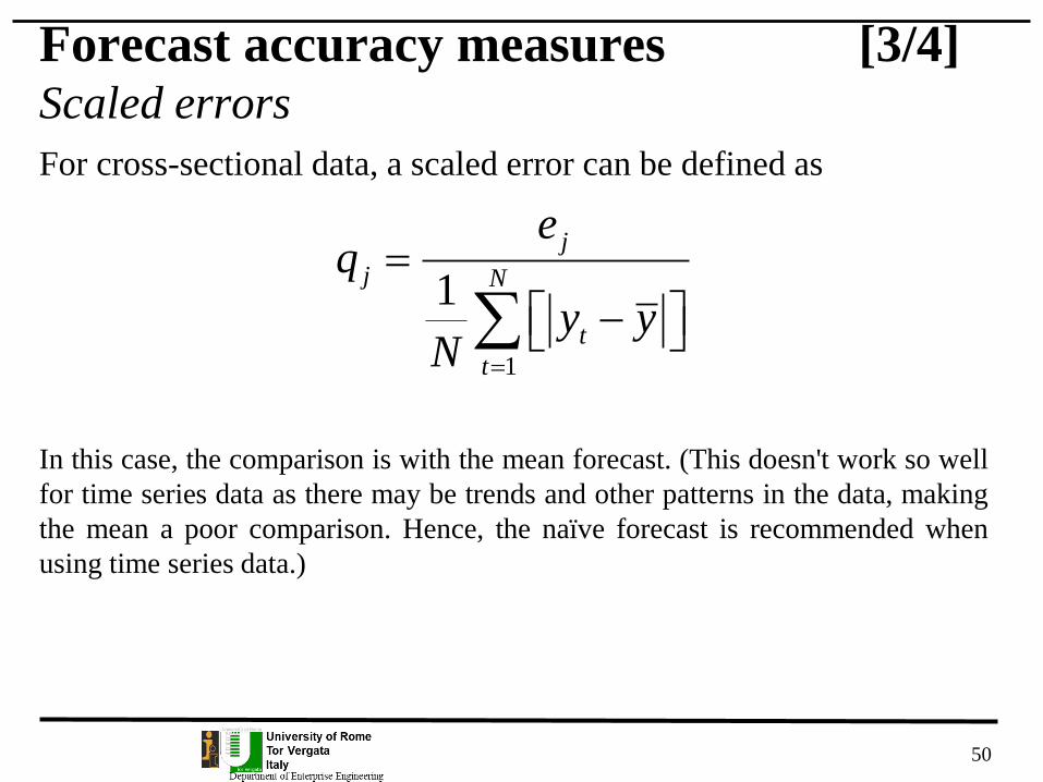
For cross-sectional data, a scaled error can be defined as
In this case, the comparison is with the mean forecast. (This doesn't work so well
for time series data as there may be trends and other patterns in the data, making
the mean a poor comparison. Hence, the naïve forecast is recommended when
using time series data.)
50
Forecast accuracy measures [3/4]Scaled errors
1
1
j
j N
t
t
eq
y yN

• Mean absolute scaled error is simply
Similarly, the mean squared scaled error (MSSE) can be defined
where the errors (on the training data and test data) are squared
instead of using absolute values.
51
Evaluation forecast accuracy [4/4]Scaled errors
jMASE mean q