DOI 10.1140/epja/i2012-12158-6

Special Article – Tools for Experiment and Theory

Eur. Phys. J. A (2012) 48: 158 THE EUROPEANPHYSICAL JOURNAL A

A single-chip telescope for heavy-ion identification

G. Pasquali1,2,a, S. Barlini1,2, L. Bardelli1,2, S. Carboni1,2, N. Le Neindre3, M. Bini1,2, B. Borderie4, R. Bougault3,G. Casini2, P. Edelbruck4, A. Olmi2, G. Poggi1,2, M.F. Rivet4, A.A. Stefanini1,2, G. Baiocco3,5, R. Berjillos10,E. Bonnet6, M. Bruno5, A. Chbihi6, I. Cruceru14, M. Degerlier8, J.A. Duenas10, M. Falorsi1, E. Galichet4,13,F. Gramegna8, A. Kordyasz11, T. Kozik12, V.L. Kravchuk8, O. Lopez3, T. Marchi8, I. Martel10, L. Morelli5,M. Parlog3,14, H. Petrascu14, S. Piantelli2, E. Rosato7, V. Seredov4, E. Vient3, and M. Vigilante7

For the FAZIA Collaboration1 Dipartimento di Fisica, Universita di Firenze, via G.Sansone 1, 50019 Sesto Fiorentino (FI), Italy2 INFN, Sezione di Firenze, via G.Sansone 1, 50019 Sesto Fiorentino (FI), Italy3 LPC, IN1P3-CNRS, ENSICAEN et Universite de Caen, F-14050 Caen-Cedex, France4 Institut de Physique Nucleaire, CNRS/IN2P3, Universite Paris-Sud 11, F-91406 Orsay cedex, France5 INFN and University of Bologna, 40126 Bologna, Italy6 GANIL, CEA/DSM-CNRS/IN2P3, B.P. 5027, F-14076 Caen cedex, France7 Dipartimento di Scienze Fisiche e Sezione INFN, Universita di Napoli Federico II, I-80126 Napoli, Italy8 INFN-LNL Legnaro, viale dell’Universita 2, 35020 Legnaro (Padova), Italy9 INFN-LNS Catania, 95129 Catania, Italy

10 Departamento de Fisica Aplicada, FCCEE Universidad de Huelva, 21071 Huelva, Spain11 Heavy Ion Laboratory, University of Warsaw, ul. Pasteura 5a, 02-093 Warsaw, Poland12 Jagiellonian University, Institute of Nuclear Physics IFJ-PAN, PL-31342, Krakow, Poland13 Conservatoire National des Arts et Metiers, 75141 Paris Cedex 03, France14 “Horia Hulubei” National Institute of Physics and Nuclear Engineering, RO-077125 Bucharest, Romania

Received: 26 July 2012 / Revised: 11 September 2012Published online: 23 November 2012c© The Author(s) 2012. This article is published with open access at Springerlink.comCommunicated by N. Alamanos

Abstract. A ΔE-E telescope exploiting a single silicon chip for both ΔE measurement and scintillationlight collection has been tested. It is a Si-CsI(Tl) telescope tailored for mass identification of light chargedparticles and intermediate mass fragments. A procedure based on two different shaping filters allows forextraction of the ΔE-E information from the single silicon signal. The quality of the obtained fragmentidentification is expressed in terms of a figure of merit and compared to that of a standard ΔE-E telescope.The presented configuration could be a good candidate for the basic cell of a large solid angle array ofΔE-E telescopes, given the reduction in complexity and cost of the front-end electronics.

1 Introduction

The effort towards complete characterization of charged-particle emission in heavy-ion collisions has motivated, inthe past decades, the construction of detection arrays cov-ering almost 4π in solid angle [1–4].

In order to identify, both in charge and mass, the emit-ted nuclear fragments, detector arrays usually feature aΔE-E telescope as elemental cell. A ΔE-E telescope is amulti-detector system: the impinging particle traverses thedetectors one after the other and the energy deposited ineach detector is measured [5]. In some cases two stages areenough and the correlation between the energy ΔE lost in

a e-mail: pasquali@fi.infn.it

the first stage and the residual energy ERES deposited inthe second stage allows to identify the charge (and also themass) of nuclear fragments. However, neither fragmentsstopped in the first ΔE detector nor fragments punchingthrough the whole telescope can be uniquely identified.Therefore an overall increased thickness is needed, consist-ing of three detector stages, e.g., a gas detector, a silicondetector and a scintillator [1,3], to obtain identificationin a wider dynamic range. A CsI(Tl) scintillator is oftenemployed as residual energy detector, due to its relativelylow cost, high stopping capability and reasonable energyresolution [6,7].

Mass and charge identification of light charged parti-cles (LCP) and intermediate mass fragments (IMF) willbe particularly useful at Radioactive Ion Beam facilities

Page 2 of 10 Eur. Phys. J. A (2012) 48: 158

in view of studies focused on nuclear isospin phenomena,where the N/Z ratio of the products will be a key exper-imental observable [8–11].

A new telescope array is under construction by theFAZIA Collaboration [12]. The array is based on three-stage ΔE-E telescopes (Si-Si-CsI(Tl)). The excellent en-ergy resolution of silicon detectors is exploited to iden-tify heavy fragments stopped in the second element viathe ΔE-E technique. A key feature of FAZIA is thePulse Shape Analysis (PSA) of detector signals. PSA isemployed to identify fragments stopped in the first sil-icon [13–15], thus lowering the identification thresholdswith respect to the standard ΔE-E technique, while atthe same time avoiding the technical complications associ-ated with gas detectors. The second silicon detector (or thecombination of the two silicon detectors) and the CsI(Tl)constitute a ΔE-E telescope for identifing the most ener-getic LCP’s and IMF’s.

Part of the effort in designing FAZIA was devoted toreducing the complexity and cost of the apparatus. Tothis aim, one could use the second Si detector both asa ΔE detector and as photodiode for reading out of theCsI(Tl) scintillation light. This solution, named “Single-Chip Telescope” (SCT), was first proposed and testedtwenty years ago [16,17] (see [18] for a recent implementa-tion). In ref. [16] the SCT signals were treated with analogelectronics and peak-sensing ADC’s and the identificationcapabilities were studied for H and He isotopes only. Inthis work SCT signals have been digitized, using samplingboards developed within the FAZIA Collaboration, andstored for offline analysis. Moreover the SCT identificationcapability has been studied both for LCP’s and IMF’s.

When applied to an array covering a large solid an-gle, the main advantage of the SCT configuration is thereduced number of front-end electronics (FEE) channelswith respect to a standard ΔE-E telescope (a factor of twofor a Si-CsI(Tl) telescope), allowing for less crowded front-end, lower power dissipation in vacuum and reduction incost. As a disadvantage, a dedicated and somewhat criti-cal signal-analysis procedure is needed to extract from aunique signal the information needed for charge and massidentification.

In sect. 2 the experimental setup employed in the SCTbeam tests is illustrated. A method for extracting the ΔEand ERES information from SCT signals, based on twodifferent shaping filters, is discussed in sect. 3. Anothermethod, based on a fit procedure, will be presented ina forthcoming paper [19]. Section 4 discusses the perfor-mance obtained with the “shaper” method and comparesit with a standard telescope in which the scintillation lightis read out by a dedicated photodiode.

2 Experimental setup

The data presented in this work were collected in Cataniaat Laboratori Nazionali del Sud (LNS) of the INFN. Thebeam was 129Xe at 35A MeV impinging on a natNi target.

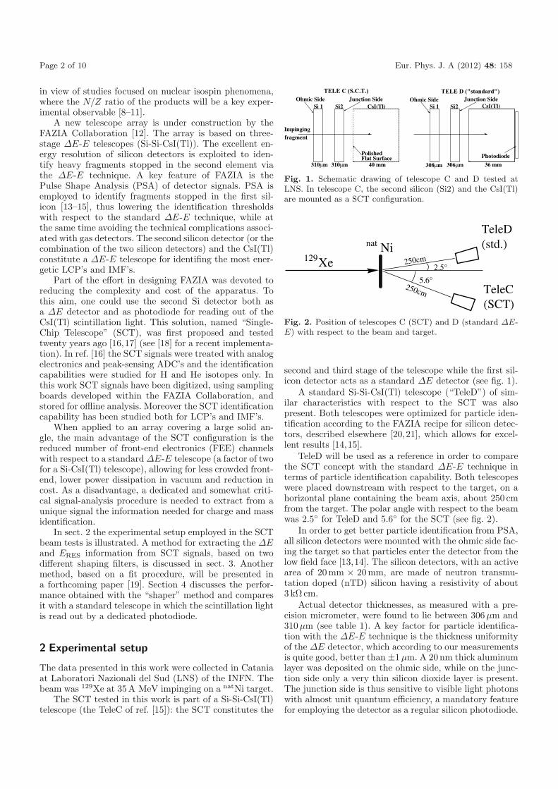
The SCT tested in this work is part of a Si-Si-CsI(Tl)telescope (the TeleC of ref. [15]): the SCT constitutes the

310 mμ 310 mμ 308 mμ 306 mμ

fragmentImpinging

TELE C (S.C.T.) TELE D ("standard")Ohmic Side Junction Side Ohmic Side Junction Side

Si 1 Si2 Si 1 Si2CsI(Tl) CsI(Tl)

PhotodiodeFlat SurfacePolished

40 mm 36 mm

Fig. 1. Schematic drawing of telescope C and D tested atLNS. In telescope C, the second silicon (Si2) and the CsI(Tl)are mounted as a SCT configuration.

129Xe

nat Ni

TeleC(SCT)

TeleD(std.)

5.6°

2.5°

250cm

250cm

Fig. 2. Position of telescopes C (SCT) and D (standard ΔE-E) with respect to the beam and target.

second and third stage of the telescope while the first sil-icon detector acts as a standard ΔE detector (see fig. 1).

A standard Si-Si-CsI(Tl) telescope (“TeleD”) of sim-ilar characteristics with respect to the SCT was alsopresent. Both telescopes were optimized for particle iden-tification according to the FAZIA recipe for silicon detec-tors, described elsewhere [20,21], which allows for excel-lent results [14,15].

TeleD will be used as a reference in order to comparethe SCT concept with the standard ΔE-E technique interms of particle identification capability. Both telescopeswere placed downstream with respect to the target, on ahorizontal plane containing the beam axis, about 250 cmfrom the target. The polar angle with respect to the beamwas 2.5◦ for TeleD and 5.6◦ for the SCT (see fig. 2).

In order to get better particle identification from PSA,all silicon detectors were mounted with the ohmic side fac-ing the target so that particles enter the detector from thelow field face [13,14]. The silicon detectors, with an activearea of 20mm × 20mm, are made of neutron transmu-tation doped (nTD) silicon having a resistivity of about3 kΩ cm.

Actual detector thicknesses, as measured with a pre-cision micrometer, were found to lie between 306μm and310μm (see table 1). A key factor for particle identifica-tion with the ΔE-E technique is the thickness uniformityof the ΔE detector, which according to our measurementsis quite good, better than ±1μm. A 20 nm thick aluminumlayer was deposited on the ohmic side, while on the junc-tion side only a very thin silicon dioxide layer is present.The junction side is thus sensitive to visible light photonswith almost unit quantum efficiency, a mandatory featurefor employing the detector as a regular silicon photodiode.

Eur. Phys. J. A (2012) 48: 158 Page 3 of 10

Table 1. Detector characteristics: telescope type, thicknessesof telescope stages, gain and full scale of the associated FEE,sampling rate and physical number of bits of the digitizers. Thefull scale energy value takes into account the position of thesignal baseline in the ADC range. Gain is given in keV/LSBunits, where LSB is the Least Significant Bit of the ADC.

Tele C Tele D

Type SCT Standard ΔE-E

thick. 310 μm 308 μm

Gain 280 keV/LSB 300 keV/LSB

Si1 F.S. 3.5 GeV 3.5 GeV

SR 100MHz 100MHz

bits 14 14

thick. 310 μm 306 μm

Gain 40 keV/LSB 160 keV/LSB

Si2 F.S. 0.5 GeV 2.0 GeV

SR 100MHz 100MHz

bits 14 14

thick. 40mm 36 mm

Gain)

see Si2

50 keV(Si)/LSB

CsI(Tl) F.S. 0.2 GeV(Si)

SR 125MHz

bits 12

A square brass collimator (20mm×20mm) was mount-ed in front of both telescopes, to prevent particles from hit-ting silicon detector borders (i.e. outside the active area).

In the SCT, the CsI(Tl) dimensions are 20mm ×20mm× 40mm; all surfaces are sanded and covered withMillipore paper except for the front face, facing the sili-con detector, which has been polished, making it opticallytransparent: scintillation photons can reach the photosen-sitive surface of the silicon detector and be collected (seefig. 1).

The TeleD features a 20mm×20mm×36mm CsI(Tl)scintillator with photodiode read-out. The front face ofthe CsI(Tl) is covered with aluminized Mylar, 2μm thick;the sides are sanded and covered with Millipore paper; therear face has been polished to make it optically transpar-ent and glued to a 18mm×18mm active area photodiode(by Hamamatsu Photonics).

Each silicon detector is connected to a PACI [22]preamplifier with charge and current outputs, both drivenby differential output buffers. Signals from the PACI arebrought out of the vacuum chamber to the digitizingboards through 8 m long differential cables (BELTENTwinax 9271, characteristic impedance 120Ω). Also thephotodiode of TeleD is connected to a dedicated PACIpreamplifier.

The present FAZIA digitizing boards feature two chan-nels (one for the charge and one for the current outputof the PACI). Only charge signals have been analyzed inthis work. The analog input stage exploits a 3-pole low-pass anti-aliasing filter (Sallen-Key configuration, Besselfrequency response [23]). The ADC (LTC2254 by LinearTechnology [24]) has a 100MHz sampling rate and 14

Time (ns)4000 5000 6000 7000 8000 9000

Am

plit

ud

e (a

.u.)

0

500

1000

1500

2000

Si component

CsI component

Baseline

O E=700 MeV16

Fig. 3. SCT output signal for a 700 MeV 16O fragment. Pole-zero cancellation of the decay of the charge preamplifier hasbeen applied.

physical bits. The effective number of bits of the customboard is ≈ 11.2. In the present experiment, FAZIA boardshave been used for the signals of the Si detectors.

The PACI output of the photodiode has been sampledby a digitizing board developed at INFN-Florence [25] fea-turing a 12 bit ADC with 125MHz sampling rate. Detec-tor characteristics, sampling rates and bit resolutions aresummarized in table 1.

The SCT scintillation light contributes to the signalof the second silicon detector. As an example, a digitizedSCT signal is shown in fig. 3. The signal refers to an 16Oof 700MeV total energy which crossed the Si chip and wasstopped in the CsI(Tl). A “pretrigger” portion, a few μslong, is acquired for every signal: it is used for the offlinecalculation of the baseline that is needed for signal ampli-tude estimation [26]. After the baseline portion (ending atabout 4.9μs in fig. 3) a steep rise is observed (rise time≈ 50 ns), associated with energy deposited directly in thesilicon. The superimposed slower component due to thecollection of scintillation light from the CsI(Tl) can beeasily recognized.

3 Data analysis with “shapers” method

3.1 “Shapers” method basic principle

In the SCT, the charge carriers in the silicon (i.e. electron-hole pairs) result either from the direct ionization of par-ticles or from collection of scintillation photons: let us callQI the charge associated with direct ionization and QL

that associated with the produced photons. Then QI isproportional to the energy ΔE deposited by the particlein the silicon while QL is proportional to the residual en-ergy ERES, i.e. the energy deposited by the particle inthe CsI(Tl) scintillator. Both QI and QL contributionsare integrated by a single PACI charge preamplifier, thuscombining in the same signal the ΔE and the ERES infor-mation.

It is known that the decay of CsI(Tl) scintillation lightas a function of time can be described by the sum of twoexponentials with different time constants: a fast time con-stant τf and a slow time constant τs. As shown in fig. 3,

Page 4 of 10 Eur. Phys. J. A (2012) 48: 158

charge collection in the Si detector and light emission inthe scintillator have quite different time scales: both τf

and τs are longer than the typical charge collection timein the silicon.

The different time scales make it possible to disentan-gle ΔE and ERES. This task can be accomplished, e.g.,by using analog shapers with different time constants, asin ref. [16]. A similar treatment can also be implementedon digitized waveforms: the digitized signal is duplicatedand the two copies are processed via different digitalshapers with different time constants. The data presentedin this paper have been processed with semi-Gaussian fil-ters. Using other filters (e.g., trapezoidal shapers), givespractically the same results, provided that the time re-sponse of the filters is suitably optimized. In the following,the shaper with the shorter time constant will be called“short” shaper, the other will be called “long” shaper.

Let us call S and L the peak amplitudes of the shortand long shaped signals, respectively1. Possible model es-timates of these amplitudes are S and L, defined as

S = QI + αQL; L = QI + βQL, (1)

where a unit conversion factor is assumed between col-lected charge and shaper amplitude. Here we have as-sumed that the peaking times of the two shapers are muchlonger than the collection time of the electron-hole pairsin silicon, so that the charge QI is totally collected. Thecoefficients α and β, on the contrary, represent the twodifferent fractions of QL contributing to S and L. Thesefractions depend on the magnitude of the chosen shap-ing constants with respect to the scintillation time con-stants τf and τs. For the CsI(Tl) scintillators employedduring the FAZIA tests a good estimate is τf � 750 nsand τs � 5μs.

Solving eqs. (1) for QI and QL one gets

QI =β

β − α

(S − α

βL)

; QL =1

β − α

(L − S

). (2)

To simplify the treatment one might consider a shortpeaking time TS � τf and a long peaking time TL � τs,a choice which would lead to α = 0 and β = 1 in eqs. (1)and (2). However this is not practical.

In fact, electronic noise must be taken into account: TS

values lower than about 400 ns produce a too low signal-to-noise ratio because of the unavoidable high-frequencynoise at the output of the preamplifier. Moreover, TL islimited by the finite length of the digitized signal (about30μs) and by the unavoidable low-frequency noise of thepreamplifier. So a viable compromise has to be found. Inthis work, the short shaper has a peaking time TS = 700 nsand the long shaper has a peaking time TL = 8μs. Adigital pole-zero cancellation of the exponential decay ofthe PACI preamplifier is performed on all signals beforeapplying the shaping filters.

1 We call the shaper amplitudes S and L (for “short” and“long”), instead of F and S (for “fast” ans “slow”) as inref. [16]. We reserve the terms “fast” and “slow” for the twocomponents of CsI(Tl) scintillation light.

0 1000 2000 3000 4000 5000 6000 7000 8000

1000

2000

3000

4000

5000

6000

7000

8000

L [a.u.]S

[a.

u.]

0 500 1000

500

1000

Direct

Ioniza

tion (n

o CsI)

Scintillation (no Si)

Fig. 4. Short shaper amplitude, S, versus long shaper am-plitude, L. The inset shows an expanded view of the low en-ergy part. The direct ionization and the scintillation lines areevidenced: all events must fall between these two lines (seeref. [16]). Counts are plotted on a logarithmic scale.

Figure 4 shows an example of the experimental S vs.L correlation. Events with QL = 0 lie along the top bor-der of the S vs. L correlation (“direct ionization” line inthe inset in fig. 4). Events with QI = 0 (e.g., cosmics,neutrons, gammas) fall along the bottom border (“scintil-lation” line). Applying eqs. (2) to the data, we can recon-struct the ΔE and ERES information (in arbitrary units)as follows:

ΔE ∝ S − KLL, ERES ∝ L − KSS, (3)

where KL = α/β and KS = 1. The KL and KS coefficientscan be adjusted, by trials and errors, until the events withQL = 0 become parallel to the ordinate axis and thosewith QI = 0 become parallel to the abscissa. As a resultof such an adjustment, ΔE vs. ERES plots like that shownin fig. 5 are obtained (where KL = 0.4 and KS = 1.02).

In figs. 4 and 5, events associated with IMF stoppedin the silicon are included. Actually, they overlap with thefamiliar ΔE-E correlation, as it clearly appears in fig. 5.The effect is due to the relatively long time needed forcollecting the direct ionization of IMF and heavier frag-ments: the short and the long shaper, having different timeconstants, actually perform a PSA on Si-stopped ions (thealmost vertical lines associated with different Z values canclearly be recognized on the left in fig. 5). These eventsmust first be recognized and excluded from the analysisin order to select proper Si-CsI(Tl) events. Their presencewas not noticed in ref. [16], probably due the low statisticsaccumulated in the IMF part of the spectra (see sect. 3.2).

The KS value needed to get the correlation of fig. 5is greater than the expected unit value. This is due to

Eur. Phys. J. A (2012) 48: 158 Page 5 of 10

0 200 400 600

1000

2000

3000

4000

5000

S [a.u]SL - K

L [

a.u

.]L

S -

K

Z=4

Z=10

Z=15

Fig. 5. Reconstructed ΔE-ERES plot. The constants KS andKL have been adjusted (KS = 1.02, KL = 0.4) to get theproper look of the correlation (see sect. 3.1). The ridge rapidlyrising from the origin and the vertical lines in the upper leftpart are associated with fragments stopped in the silicon.Counts are plotted on a logarithmic scale.

the finite rise time of the direct ionization signal, whichsuffers some ballistic deficit when processed by the shortshaper with respect to the long one [27]. The minimum ofthis rise time is determined by the FEE. Indeed a ballisticdeficit of about 2% has been estimated for the short shaperby studying its response to signals produced in the firstsilicon, Si1, which are due to direct ionization only anddo not contain any CsI(Tl) contribution. Therefore, in thefirst of eqs. (1) the coefficient of QI should be 0.98 insteadof 1.

3.2 Recognizing fragments stopped in Si detector

The shapes of the charge signals are quite different for ionsstopped in the Si detector with respect to ions producingscintillation also in the CsI(Tl). A particle stopped in Sifeatures a steep almost linear leading edge (as shown inthe top panel of fig. 6 for a 16O fragment of 285MeVkinetic energy). On the contrary, when scintillation lightcontributes to the pulse shape, the topmost part of theleading edge presents a noticeable slowing down, as shownin the bottom panel of fig. 6. Events can be sorted intwo classes (“stopped in Si” and “stopped in CsI(Tl)”) onthe base of their different shapes. For example, one coulddefine a parameter Δtsym as

Δtsym = (T90% − T80%) − (T80% − T50%), (4)

where TN% is the time at which the leading edge reachesN% of the maximum amplitude. The rationale behind theΔtsym parameter is illustrated in fig. 6 where the circles

Am

plit

ud

e (a

.u.)

0

2000

4000 O stopped in Si16285MeV

=-2nssym tΔ

Time (ns)4000 5000 6000 7000

Am

plit

ud

e (a

.u.)

0

1000

2000O stopped in CsI16700MeV

=90nssym tΔ

Fig. 6. Typical signal shapes for the two event classes(“stopped in Si” and “stopped in CsI(Tl)”). Top panel: chargesignal produced by a 16O with 285MeV kinetic energy, stoppedin the silicon. Bottom panel: charge signal produced by a 16Owith 700 MeV kinetic energy, stopped in the CsI(Tl). Full cir-cles plotted on the leading edge correspond to the amplitudefractions of 50%, 80% and 90%, used to calculate Δtsym, andto the associated times, namely T50%, T80% and T90% (seesect. 3.2).

mark the signal amplitudes at the adopted values T50%,T80% and T90%. When the amplitude of the silicon com-ponent is greater than 50% of the full amplitude, the firstpoint (the one at T50%) lies on the steepest part of theleading edge. If there is no CsI(Tl) contribution to thesignal, the other two points will also lie on the steep rise,giving low Δtsym values (e.g., Δtsym = 0 for an exactlylinear leading edge and equally distanced fractions). If thesignal slows down in the upper part, as for particles reach-ing the CsI(Tl), Δtsym will tend to become positive. Withthe chosen fractions, particles stopped in the silicon giveΔtsym < Δt0 while particles stopped in the CsI(Tl) givevalues Δtsym > Δt0, with Δt0 ≈ 4.1 ns.

When the silicon contribution amounts to less than50% of the final amplitude, Δtsym alone does not allow aclean separation. For those events, however, a simple cri-terium based on signal rise time (10% to 90% of maximumvalue) can be adopted, since the slow CsI(Tl) componentdominates the leading edge shape. To summarize, eventsare recognized as

– “stopped in CsI(Tl)” if (Δtsym > Δt0) or (signal risetime > 600 ns);

– “stopped in Si” if (Δtsym < Δt0) and (signal rise time< 600 ns).

Data on charge and mass identification of “stopped inSi” fragments will not be presented in this paper. However,the PSA techniques already discussed in ref. [15] have alsobeen applied to “stopped in Si” events, obtaining resultscomparable to those of ref. [15].

Page 6 of 10 Eur. Phys. J. A (2012) 48: 158

0 100 200 300 400 500 600

20

40

60

80

100

120

140

160

Light Output [a.u]

E [

MeV

]Δ

BeBC

N

O

0 100 20040

60

80

B

C

N

Fig. 7. Reconstructed ΔE (in MeV) vs. CsI(Tl) light output(a.u.) for IMFs. In the inset, an expanded view of the regionwhere carbon isotopes are better resolved is shown. Counts areplotted on a logarithmic scale.

0 50 100 150 200 250 300 350

5

10

15

20

25

Light Output [a.u]

E [

MeV

]Δ

He

Li

0 50 100 150 200

1

2

Fig. 8. Reconstructed ΔE (in MeV) vs. CsI(Tl) light out-put (a.u.) for LCPs. In the inset, an expanded view of highestenergy hydrogen isotopes is shown. Counts are plotted on alogarithmic scale.

3.3 “Shaper” method results

Using the selection criteria of sect. 3.22, one can producethe “cleaned up” ΔE-ERES correlations shown in figs. 7and 8 where ΔE and ERES are calculated as in fig. 5.Knowing the detector thickness, an energy calibration canbe obtained exploiting the punch through points in the

2 A residual contamination of the ΔE-ERES correlations bystopped particles remains for hydrogen and helium isotopes.However, since these events fall on the ΔE axis in the ΔE-E correlation, they can be easily discarded. In fact, the fastcollection time for the charge produced by a LCP makes S = Land therefore QL = 0, see eqs. (2).

uncalibrated ΔE(Si1) vs. ΔE(SiSCT) correlation and thecorresponding energy values obtained from energy loss ta-bles [28]. The ΔE value in figs. 7 and 8 has been calibratedin energy in this way. A possible cause of non-linearity inthe ΔE energy calibration, related to the response of theshapers to the SCT signal, has been identified: it is dis-cussed in the appendix.

The maximum energy deposited in the CsI(Tl) was≈ 100MeV for H, ≈ 300MeV for Li and Be, ≈ 400MeVfor B and C. It would be possible to calibrate in energy the“Light Output” axis —exploiting the calibrated ΔE(Si1)and ΔE(SiSCT) values— to obtain full calibrated energyspectra. This has not been attempted in this paper, butwe plan to perform the relevant energy calibration whenthe detector is used in real experiments.

Element resolution is obtained in the whole range al-lowed by the FEE saturation amplitude (up to Z ≈ 13).A reasonable mass separation is achieved for LCP’s andlow-Z IMF’s (up to Be). However, only marginal mass res-olution is achieved for boron and carbon isotopes: differentmasses can be recognized only in a small energy range. Nomass resolution is achieved for Z > 6.

The ΔE-ERES correlations have been subsequently lin-earized, extracting a particle identification (PID) parame-ter to quantitatively estimate the isotopic resolution. Re-sults of this analysis will be shown in sect. 4.1 and com-pared with a similar analysis performed on TeleD.

4 Detector performance

4.1 Particle identification

Particle identification capabilities can be quantitativelyestimated by linearizing the correlations of fig. 7 and fig. 8in order to extract a particle identification parameter PID.For a comparison of the SCT performance with that of astandard ΔE-E telescope of similar characteristics, thecorresponding ΔE-E correlations have been obtained forTeleD.

Figure 9 shows the PID spectra for isotopes of elementsup to carbon. Comparing the TeleD data (solid black line)and the SCT data (dotted red line) one can notice a com-parable performance for LCP’s, while for Z > 2 the SCTidentification is significantly worse.

The information given in fig. 9 can be made more quan-titative by estimating a “figure of merit” (FoM). For a pairof neighboring peaks, the FoM is defined [29] as

FoM =|C1 − C2|

FWHM1 + FWHM2, (5)

where C1 and C2 are the centroids of the two peaks andFWHM1 and FWHM2 are the corresponding full widthsat half maximum. Centroids and full widths at half max-imum have been estimated from a multiple Gaussian fit.We conventionally consider two isotopes as well separatedif FoM ≥ 0.7 [14,15].

In order to check how the particle identification de-grades with energy, in fig. 10 the FoM for different isotope

Eur. Phys. J. A (2012) 48: 158 Page 7 of 10

PID1 1.1 1.2 1.3

cou

nts

1

10

210

310

410Z=1

PID1.8 1.9 2 2.1 2.2 2.3

cou

nts

1

10

210

310

410Z=2

PID2.8 2.9 3 3.1 3.2

cou

nts

1

10

210

Z=3

PID3.6 3.7 3.8 3.9 4 4.1

cou

nts

1

10

210

Z=4

PID4.8 4.9 5 5.1 5.2

cou

nts

1

10

210

Z=5

PID5.8 5.9 6 6.1 6.2 6.3

cou

nts

1

10

210

Z=6

Fig. 9. Particle identification (PID) parameter obtained fromthe ΔE-E correlations of figs. 7 and 8: no cut on particle en-ergy has been applied. Solid (black) line: PID spectra fromthe standard telescope (TeleD). Dotted (red) line: PID spectrafrom the SCT, downscaled by a factor of three. Dash-dotted(blue) line: PID spectra obtained by mixing together the ΔEand ERES signals of TeleD to mimic a SCT (see sect. 4.2),downscaled by a factor of nine.

pairs is plotted as a function of the estimated particle en-ergy, EINC, at the entrance of the silicon of the SCT. Todo so, first PID spectra have been obtained for adjacentintervals of light output of the CsI(Tl) and the FoM val-ues of various isotope pairs have been calculated in eachslice. Then for each slice and isotope pair (i.e. for eachpoint in fig. 10) the average EINC value of the lower-massisotope has been estimated from the ΔE measured by Si1and from energy loss tables [28].

As already noticed in fig. 9, the FoM values for LCP’sconfirm that a comparable performance can be obtainedfrom the standard telescope (full circles) and the SCT(triangles). For IMF’s, on the contrary, the SCT is not asgood as the standard telescope, especially at low energies.

4.2 Reconstruction procedure and isotopicidentification

The worse isotopic resolution of the SCT could be due justto the reconstruction procedure itself. In order to eval-

(MeV)INCE0 50 100

Fo

M

1

2

3

p - d

(MeV)INCE0 50 100

d - tTeleD

TeleD SCT-like

SCT

(MeV)INCE0 100 200 300

Fo

M

0.5

1

1.5

2

Li7Li - 6

(MeV)INCE0 100 200 300

Be10Be - 9

(MeV)INCE0 200 400

C13C - 12

Fig. 10. Figure of Merit (FoM) values for different isotopepairs as a function of the average incident energy EINC of thefirst isotope (p, d, 6Li, 9Be, 12C, respectively) before enter-ing the SCT. The results are for the SCT (triangles) and fora standard telescope (TeleD). For the latter, Si and CsI(Tl)signals have been treated separately (full dots) or mixed in asingle composite signal (open dots), see sect. 4.2. The incidentenergy is calculated on the basis of the ΔE energy measuredby the preceding first silicon. Each point corresponds to an in-terval of CsI(Tl) Light Output values (see sect. 4.1 for details).The 0.7 limit is evidenced by the horizontal (red) line. Errorbars refer only to statistical uncertainties.

uate the effect of the SCT reconstruction procedure onisotopic identification, we have built “SCT-like” signalsfrom the Si2 and CsI(Tl) signals of TeleD. The two sig-nals have been first properly scaled in amplitude to takeinto account the different gains of the associated electron-ics. Then their leading edges have been time-aligned. TheCsI(Tl) signal sampling period (originally 8 ns) has beenmade equal to that of the Si signal (10 ns) via interpo-lation. Finally the two signals have been added sampleby sample. The resulting signal looks very much like theproper SCT signal already presented in figs. 3 and 6. TheADC noise prevents a proper alignment of Si2 and CsI(Tl)signals of TeleD for hydrogen isotopes, especially at thehighest measured energies: therefore we will not presentresults for Z = 1 isotopes.

Signals obtained in such a way have been analyzedusing the same reconstruction procedure as for the ac-tual SCT signals. ΔE-ERES correlations similar to thoseof figs. 7 and 8 have been produced and linearized. It isthus possible to obtain the PID spectra shown by thedash-dotted (blue) histograms in fig. 9. A worsening ofthe particle identification capability due to the reconstruc-tion procedure is apparent when comparing PID obtainedwith the standard treatment (solid black line) and withthe SCT-like analysis (dash-dotted blue line).

To be more quantitative, the FoM for neighboring iso-topes is plotted in fig. 10 (open circles). Comparing theFoM values obtained for TeleD with the two methods (fulland open circles in fig. 10), we find that the reconstruc-tion procedure worsens the resolution particularly at low

Page 8 of 10 Eur. Phys. J. A (2012) 48: 158

energy. One could then attribute the worse FoM valuesobtained at the lowest energies for the SCT, with respectto the TeleD standard, to the need to extract the informa-tion from a single signal. It is well known that the isotopicresolution is influenced more by the resolution in ΔE thanin ERES. In a Si-CsI(Tl) telescope, the ERES measurementis certainly more affected by statistical fluctuations thanthe ΔE measurement, due to the lower number of carriers.In fact, taking into account light collection efficiency, scin-tillation photons in CsI(Tl) have an energy cost at leasta factor of 20 larger than electron-hole pairs in Si. WhenΔE is obtained from a single signal combining the ΔEand ERES information, the larger fluctuations in ERES

can negatively affect the reconstructed ΔE value, thusspoiling the isotopic resolution with respect to a standardtelescope where ΔE and ERES are treated separately.

In the PID spectra of fig. 9, TeleD and SCT presentsimilar isotopic separation for hydrogen isotopes even atthe lowest energy. In fact, as shown in fig. 10, at the lowestenergy the SCT has a better isotopic separation for hy-drogen isotopes than for IMF’s. A possible interpretationof this result is the following: the FEE electronics of theSCT features a better S/N ratio than TeleD, due to thehigher gain of the associated PACI preamplifier. In fact,the energy range allowed by the FEE was about 500MeVfor the SCT and about 2GeV for the Si2 of TeleD. ForLCP’s, where the Si signal has low amplitude, the elec-tronic noise of the digitizer affects the ΔE resolution ofTeleD giving a worse isotopic identification. The SCT isless affected by such noise due to the higher gain of itspreamplifier, thus obtaining, in spite of the reconstructionprocedure, a performance similar to that of the standardtelescope. The latter, however, thanks to the lower gain,features a much wider dynamic range (up to the highest Zvalues available in the experiment, while the FEE of theSCT saturates for Z ≈ 13).

At higher energy, both for hydrogen isotopes and IMF’s,TeleD and SCT are quite similar in performance, givingFoM’s under the 0.7 limit.

5 Conclusions

A ΔE-E telescope exploiting the SCT concept has beentested and compared to a standard ΔE-E telescope of sim-ilar characteristics. Both are three-stage Si-Si-CsI(Tl) tele-scopes. In the SCT the scintillation light from the CsI(Tl)is read out by the same Si chip acting as second ΔE ele-ment. Detector signals from the preamplifiers are digitizedusing custom FEE and stored on disk. Information aboutΔE and ERES is extracted using a numerical reconstruc-tion procedure based on two digital shaping filters withdifferent time constants, acting on digitized signals.

The particle identification capability of the SCT andassociated reconstruction procedure has been evaluatedfor different isotopes at various energies and it has beencompared with that of the standard telescope. Similar per-formances are obtained for LCP’s. For IMF’s, the standardtelescope gives better isotopic identification.

Time (ns)2000 3000 4000

Am

plit

ud

e (a

.u.)

0

0.2

0.4

0.6

0.8

1

Time (ns)2000 3000 4000

Am

plit

ud

e (a

.u.)

0

0.2

0.4

0.6

0.8

Si+CsI

Si

CsI

Fig. 11. Different peaking times of the short shaper for the Siand CsI(Tl) components and their effect on the overall peakvalue. Top panel: simulated SCT signal (solid line) for a parti-cle punching through the Si detector and stopped in CsI(Tl).The Si (dashed line) and CsI(Tl) (dotted line) components ofthe signal are also separately plotted. Bottom panel: responseof the short semi-Gaussian shaper to the signals shown in theupper panel. The arrow marked Si (CsI) corresponds to themaximum shaper amplitude for the Si (CsI) component. Thearrow marked Si+CsI indicates the sum of the two maximumamplitudes.

The effect of the reconstruction procedure has beenstudied for IMF’s, analyzing SCT-like signals obtained bysuitably scaling and adding the standard telescope Si andCsI(Tl) signals. It has been found that adding the signalsand then applying a reconstruction procedure indeed pro-duces worse isotopic resolution for IMF’s of relatively lowenergy although at higher energy the standard telescopeand the SCT give comparable results.

Alternative reconstruction procedures can also be de-vised. A procedure based on a fit of the SCT signal shapesis presently under study: its result will be published in aforthcoming paper [19].

Appendix A. Correction for shapernon-linearity

If eqs. (2) are valid, then the QI and QL values reflectthe actual charge created in the silicon depletion volumeby direct ionization and scintillation light, respectively.In particular, ΔE(SiSCT) (given by the first of eqs. (3)),which is an estimate of QI , should exhibit a linear be-haviour with deposited energy as expected for a standardSi detector. One can check this assumption by calibrat-ing in energy the two silicon detectors and comparing theresulting ΔE(Si1) vs. ΔE(SiSCT) correlation with the pre-dictions of energy loss tables [28].

This has evidenced a discrepancy for energetic parti-cles that punch through the second silicon detector andare stopped in the CsI(Tl). The ΔE (SiSCT) value seems

Eur. Phys. J. A (2012) 48: 158 Page 9 of 10

more and more underestimated as the total energy of theparticle increases. Actually, eqs. (1) do not take into ac-count that the maximum amplitude for the actual com-posite SCT signal is not equal to the sum of the maximumvalues one would obtain for the Si (direct ionization) andCsI(Tl) (scintillation) components separately. This is dueto the different peaking times of the shaper when appliedto the two components. The effect exists for both shapers,but it is greater for the short shaper. In fact its shap-ing constant is shorter than both CsI(Tl) time constants(τf � 750 ns and τs � 5μs) while it is greater than thecollection time for charge directly produced in the silicon:therefore its peaking times for Si and CsI(Tl) componentsare the most different.

Our shapers are linear time-invariant systems. Theirresponse to the whole SCT signal is therefore equal to thesum of their responses to the two separate components.In fig. 11 (top panel) a simulated SCT signal (solid line)is shown together with its Si (dashed line) and CsI(Tl)(dotted line) components. Responses of the short shaperto the full signal and separately to its two components arealso shown in fig. 11 (bottom panel). Summing the peakvalues of the separate responses (evidenced by arrows inthe bottom panel of fig. 11) one gets a value which isgreater by about 10% than the response to the whole sig-nal: in fact, when the response to the whole signal arrivesat its maximum, the response to the CsI(Tl) componenthas not yet reached its peak amplitude. The magnitudeof the effect depends on the relative weights of the siliconand CsI(Tl) components, thus producing a non-linearityin the response as a function of energy. With increasingkinetic energy, the CsI(Tl) contribution to the SCT signalincreases and this non-linear behaviour of the maximumamplitude of the shaper must be taken into account.

A correction for this effect can be estimated, basedon the known shaper response. SCT signals have beensimulated for different values of the QI/(QI + QL) ratio.Different values of the ratio Qs/Qf between the slow andfast CsI(Tl) components have also been used (namely 0.2,0.5 and 1.0). The ratio R = S/S = S/(QI + α QL) be-tween the simulated short shaper peak amplitude and thepredictions of eqs. (1) has been calculated. The α valuecorresponds to the output amplitude of the short shaperwhen applied to a simulated SCT signal with QI = 0 andQL = 1.

It is useful to study R as a function of XS = QI/(QI +α QL). XS takes values between XS = 0, when no directionization in Si is produced (QI = 0), and XS = 1, whenthere is no contribution from CsI(Tl) scintillation light(QL = 0): at the extremes of the interval spanned by XS

one expects R = 1. In fact, for XS = 0 and XS = 1 thefull signal has only one component and thus there are notwo distinct peaking times. The simulation shows that Rattains a minimum for XS ≈ 0.5. For instance, for theshort shaper employed in this work and for Qs/Qf = 0.2(a value typical for IMF’s [30]), R assumes a miminumvalue of about 0.87. The behaviour of R as a function ofXS is well described by a second order polynomial, whoseparameters can be extracted with a fit and then used in

data analysis to correct the experimental S values, to re-store the validity of eqs. (1). We found that the maximumvalue of the correction to be applied to the short shaperamplitude is 13%, as in the previous example, almost in-dipendently of the assumed Qs/Qf ratio.

In order to apply the correction to experimental data,an estimate of XS is needed for each event. As a firstapproximation, one could assume the validity of eqs. (2),thus deriving for XS the following expression

XS =QI

QI + α QL� S − KL L

(1 − KL) S, (A.1)

where S and L are the experimental peak values. KL (=α/β) must be experimentally estimated from the ΔE-Ecorrelations (see sect. 3.1).

A similar correction can be applied to the long shaper,though in this case the maximum correction is about 2%,because of the longer peaking time.

Open Access This is an open access article distributedunder the terms of the Creative Commons AttributionLicense (http://creativecommons.org/licenses/by/3.0), whichpermits unrestricted use, distribution, and reproduction in anymedium, provided the original work is properly cited.

References

1. J. Pouthas et al., Nucl. Instrum. Methods A 357, 418(1995) doi:10.1016/0168-9002(94)01543-0.

2. S. Aiello et al., Nucl. Phys. A 583, 461 (1995) doi:10.1016/0375-9474(94)00705-R.

3. A. Moroni et al., Nucl. Instrum. Methods A 556, 516(2006) doi:10.1016/j.nima.2005.10.123.

4. S. Wuenschel et al., Nucl. Instrum. Methods A 604, 578(2009) doi:10.1016/j.nima.2009.03.187.

5. D.A. Bromley, IRE Trans. Nucl. Sci. 9, 135 (1962) doi:10.1109/TNS2.1962.4315986.

6. W.G. Gong et al., Nucl. Instrum. Methods A 268, 190(1988) doi:10.1016/0168-9002(88)90605-5.

7. M. Parlog et al., Nucl. Instrum. Methods A 482, 693(2002) doi:10.1016/S0168-9002(01)01712-0.

8. E. Galichet et al., Phys. Rev. C 79, 064614 (2009) doi:10.1103/PhysRevC.79.064614.

9. T.X. Liu et al., Phys. Rev. C 76, 034603 (2007) doi:10.1103/PhysRevC.76.034603.

10. M. Di Toro et al., Eur. Phys. J. A 13, 155 (2002) doi:10.1140/epja1339-28.

11. Ad.R. Raduta, F. Gulminelli, Phys. Rev. C 75, 044605(2007) doi:10.1103/PhysRevC.75.044605.

12. FAZIA Project: http://fazia2.in2p3.fr/spip.13. M. Mutterer et al., IEEE Trans. Nucl. Sci. 47, 756 (2000)

doi:10.1109/23.856510.14. L. Bardelli et al., Nucl. Instrum. Methods A 654, 272

(2011) doi:10.1016/j.nima.2011.06.063.15. S. Carboni et al., Nucl. Instrum. Methods A 664, 251

(2012) doi:10.1016/j.nima.2011.10.061.16. G. Pasquali et al., Nucl. Instrum. Methods A 301, 101

(1991) doi:10.1016/0168-9002(91)90742-9.

Page 10 of 10 Eur. Phys. J. A (2012) 48: 158

17. G. Prete et al., Nucl. Instrum. Methods A 315, 109 (1992)doi:10.1016/0168-9002(92)90689-2.

18. J. Lukasik et al., EPJ Web of Conferences 31, 00032 (2012)doi:10.1051/epjconf/20123100032.

19. G. Pasquali et al., in preparation.20. L. Bardelli et al., Nucl. Instrum. Methods A 605, 353

(2009) doi:10.1016/j.nima.2009.03.247.21. L. Bardelli et al., Nucl. Instrum. Methods A 602, 501

(2009) doi:10.1016/j.nima.2009.01.033.22. H. Hamrita et al., Nucl. Instrum. Methods A 531, 607

(2004) doi:10.1016/j.nima.2004.05.112.23. L. Bardelli et al., Nucl. Instrum. Methods A 491, 244

(2002) doi:10.1016/S0168-9002(02)01273-1.24. http://www.linear.com/.

25. G. Pasquali et al., Nucl. Instrum. Methods A 570, 126(2007) doi:10.1016/j.nima.2006.10.008.

26. L. Bardelli et al., Nucl. Instrum. Methods A 560, 524(2006) doi:10.1016/j.nima.2005.12.250.

27. B.W. Loo, F.S. Goulding, D. Gao, IEEE Trans. Nucl. Sci.NS-35, 114 (1988) doi:10.1109/23.12686.

28. F. Hubert et al., Atom. Data Nucl. Data Tables 46, 1(1990) doi:10.1016/0092-640X(90)90001-Z.

29. R.A. Winyard, J.E. Lutkin, G.W. McBeth, Nucl. In-strum. Methods 95, 141 (1971) doi:10.1016/0029-554X(71)90054-1.

30. F. Benrachi et al., Nucl. Instrum. Methods A 281, 137(1989) doi:10.1016/0168-9002(89)91225-4.