a stable scaling of newton-schulz for improving … · scaled newton-schulz for matrix sign...

Preprint ANL/MCS-P5059-0114

A STABLE SCALING OF NEWTON-SCHULZ FOR IMPROVING THESIGN FUNCTION COMPUTATION OF A HERMITIAN MATRIX

JIE CHEN∗ AND EDMOND CHOW†

Abstract. The Newton-Schulz iteration is a quadratically convergent, inversion-free method forcomputing the sign function of a matrix. It is advantageous over other methods for high-performancecomputing because it is rich in matrix-matrix multiplications. In this paper we propose a variant forHermitian matrices that improves the initially slow convergence of the iteration. The main idea isto scale the iteration to have steeper derivatives of the mapping function at the origin such that theconvergence of the eigenvalues with small magnitudes is accelerated. The scaling is stable based ona backward stability result of Y. Nakatsukasa and N. J. Higham. Generally, the number of iterationsis reduced by half compared with standard Newton-Schulz. With proper shifts of the matrix, thisnumber may be further reduced. We demonstrate numerical calculations with matrices of size up toapproximately 105 on medium-sized computing clusters and also apply the algorithm to electronicstructure calculations.

Key words. Matrix sign function, Newton-Schulz iteration, electronic structure calculation

AMS subject classifications. 65F60

1. Introduction. We are interested in numerically computing the matrix signfunction

S = sign(A)

for a matrix A ∈ Cn×n with no eigenvalues lying on the imaginary axis. The scalarsign function sign(z) takes value +1 when <(z) > 0 and −1 when <(z) < 0. In thispaper we focus on the Hermitian case, where a simplified definition of the matrix signfunction is

sign(A) = U · diag(sign(λ1), . . . , sign(λn)) · U∗,

with U∗AU = diag(λ1, . . . , λn) being a diagonalization of A. The Hermitian caseappears in several real-life applications, such as lattice quantum chromodynamics [23,29, 10] and electronic structure calculations [28, 26]. For the latter application, thedensity matrix ρ of a molecular system with Fermi level µ is the Heaviside functionof µI −H, where H is an approximation to the Hamiltonian. Thus, one can computeρ as 1

2 [sign(µI −H) + I]. To respect the notational convention in different fields, werecycle the notation ρ, µ, and H for the discussion of matrix functions, where thedifferent meanings are clear in context.

Four iterative methods for computing sign(A) relevant to the present paper areNewton [12, 11], inverse Newton [11, 21], Halley [21], and Newton-Schulz [12, 11].Some of these methods are more frequently associated with the computation of thepolar decomposition, but since they are akin to the Pade family of approximations of

∗Mathematics and Computer Science Division, Argonne National Laboratory, Argonne, IL 60439([email protected]). Work supported by the U.S. Department of Energy, Office of Science, Officeof Advanced Scientific Computing Research, under Contract DE-AC02-06CH11357.†School of Computational Science and Engineering, College of Computing, Georgia Institute of

Technology, Atlanta, GA 30332 ([email protected]). Work supported by NSF under grant ACI-1147843.

1

2 J. CHEN AND E. CHOW

the sign function [11, Section 5.4], we can use the methods with a slight modificationfor computing the matrix sign. The iterations admit the form

Xk+1 = f(Xk), X0 = A, (1.1)

where f corresponds to different mappings. The four methods are

Newton: f(X) =1

2(X +X−1),

Inverse Newton: f(X) = 2X(I +X2)−1,

Halley: f(X) = X(3I +X2)(I + 3X2)−1,

Newton-Schulz: f(X) =1

2X(3I −X2).

It is not hard to see that the iterates produced by the second method are the inversesof the Newton iterates, hence the name “inverse Newton.” The first three methods areglobally convergent, with the rate being quadratic for the first two and cubic for thethird. On the other hand, Newton-Schulz is known to be convergent when ‖I−A2‖ <1, for any subordinate matrix norm. When A is Hermitian, the convergence region canbe expanded to ρ(A) <

√3, where ρ means the spectral radius. Hence, in practical

use of Newton-Schulz, one may first scale A by ρ(A). We note that in electronicstructure calculations, the McWeeny purification method [19, 16] is equivalent toNewton-Schulz.

The fact that spectral information is needed for Newton-Schulz does not neces-sarily make the method inferior to the other three globally convergent methods. Thereason is that scaling becomes a practical need for enhancing the convergence of thesemethods. Several scalings have been proposed for Newton and inverse Newton; theyall share the form

Xk+1 = f(µkXk).

For Newton, the determinantal scaling defines µk = |det(Xk)|−1/n, the spectral scal-

ing defines µk =√ρ(X−1

k )/ρ(Xk), and the norm scaling defines µk =√‖X−1

k ‖/‖Xk‖.The last two scalings are equivalent when A is Hermitian and when ‖·‖ is the 2-norm;in such a case, they are both optimal. A disadvantage is that these scalings are expen-sive to compute, because they depend on each iterate Xk. Byers and Xu [2] proposeda suboptimal scaling that requires the computation of the spectral information onlyonce. The scaling sequence reads

µ0 = 1/√αβ, µ1 =

√2√αβ/(α+ β), µk = 1/

√f(µk−1) for k = 2, 3, . . . ,

where α = ‖A‖2, β = ‖A−1‖−12 and f is the scalar Newton mapping f(µ) =

(µ + µ−1)/2. By using the Byers and Xu scaling, in exact arithmetic, at most nineiterations are needed for Newton to converge within a tolerance of 10−16 for matriceswith condition number no greater than 1016. The counterpart scaling approach forinverse Newton is derived by inverting α, β, and f in Byers and Xu.

For the Halley method, Nakatsukasa et al. [21] suggested an optimal scaling

Xk+1 = Xk(akI + bkX2k)(I + ckX

2k)−1, X0 = A/α, (1.2)

SCALED NEWTON-SCHULZ FOR MATRIX SIGN COMPUTATION 3

where α = ‖A‖2, `0 = σmin(X0), and

ak = h(`k), bk = (ak − 1)2/4, ck = ak + bk − 1,

`k = `k−1(ak−1 + bk−1`2k−1)/(1 + ck−1`

2k−1),

h(`) =√

1 + γ +1

2

√8− 4γ +

8(2− `2)

`2√

1 + γ, γ =

3

√4(1− `2)

`4.

Here, σmin denotes the smallest singular value. The scaling approach is coined DWH(dynamically weighted Halley). By using such a scaling, in exact arithmetic, at mostsix iterations are needed for Halley to converge within a tolerance of 10−16 for matriceswith condition number no greater than 1016.

Despite the above appealing mathematical properties, scalings lead to subtle nu-merical stability issues. Nakatsukasa and Higham [22] performed a comprehensiveanalysis on a general fixed-point iteration (1.1). They showed that the iterations arebackward stable when the matrix inverse is computed in a mixed backward-forwardstable manner and when f does not significantly decrease the size of any singularvalue relative to the largest one. This result explains the observation that the Newtonmethod with either spectral/norm scaling or Byers-Xu scaling is stable (see also [13]and [2]), but the inverse Newton method with a Byers-Xu-like scaling is generallynot. For the Halley method (DWH), a stable implementation is to replace (1.2) by amathematically equivalent iteration [21]:

Xk+1 =bkckXk +

1√ck

(ak −

bkck

)Q1Q

∗2, (1.3)

where [√ckXk

I

]=

[Q1

Q2

]R

is a thin QR factorization.Figure 1.1 demonstrates an example of the stability behavior of various scaled

iterations. The 20× 20 matrix A is defined as

A = Q∗DQ, (1.4a)

where Q is the orthogonal factor of a Gaussian random matrix and D is a diagonalmatrix with

diag(D) = [1,−ε, ε17/17, ε16/17, . . . , ε1/17, ε0/17]. (1.4b)

Here, ε is chosen to be 10−16 so that the matrix has a condition number 1016. Therelative error on the vertical axis is defined as

‖A−Xk(H +H∗)/2‖F /‖A‖F , where H = X∗kA.

Such an error metric originates from the polar decomposition, where H is the Her-mitian polar factor of A. The error metric accurately measures the preservation ofthe eigenspace of A in Xk. One sees that Newton with Byers-Xu scaling and Halley(DWH) with the QR implementation (1.3) can reach the level of 10−15, but inverseNewton with Byers-Xu-like scaling and Halley (DWH) with the LU implementation of


0 5 10 15 20 25 30 35 40 45 5010−20

10−15

10−10

10−5

100

105

1010

1015

1020

Newton, Byers−Xu scalingInverse Newton, Byers−Xu−like scaling

Halley, DWH with LU inverse

Halley, DWH with QR.

Scaled Newton−Schulz, unstable

Scaled Newton−Schulz, stable

Fig. 1.1. Convergence history for different scaled iterations. The matrix A is defined in (1.4).

matrix inverse (1.2) cannot. The figure also shows the results of two scaled Newton-Schulz iterations, the subject of this paper.

Generally, Newton-Schulz requires a few times more iterations to converge thando the other three methods. However, the appeal of Newton-Schulz is that it isinversion-free. The matrix-matrix multiplications therein may be expected to havebetter parallel scalability than the factorizations used for matrix inversion (e.g., LUand QR), even if the factorizations employ no pivoting. The best communicationcost of matrix-matrix multiplications is log p times smaller than that of LU and QR,where p is the number of processors [1, 5]. Moreover, the arithmetic cost of Newton-Schulz is comparable with that of the other iteration methods, counting the totalflops (see Section 4.1). Hence, Newton-Schulz has a greater potential for efficiency ina massively parallel computing setting.

In this paper, we focus on improving the initial convergence of Newton-Schulz, bynoting that a drawback of the method is that it requires a large number of iterationsbefore the quadratic convergence is seen. The derivation of the improvement is logi-cally separated in two steps. In the first step, we seek an optimal scaling by analyzingthe fixed-point mapping f of Newton-Schulz (Section 2). The key observation is thatthe initial convergence is governed by the derivative of the mapping at the origin.Thus, the optimal scaling appears in the form

Xk+1 =1

2αkXk(3I − α2

kX2k),

where αk is the smallest magnitude eigenvalue of Xk (Section 3). A recurrence for-mula can be derived for αk such that eigenvalue computations are not needed inevery iteration. Analysis suggests that the number of iterations for the optimal scal-ing is reduced by half compared with nonscaling. The same scaling approach wasindependently proposed by Rubensson [24] in the context of electronic structure cal-culations. Unfortunately, this scaling is not stable, as demonstrated by the curveannotated as “scaled Newton-Schulz, unstable” in Figure 1.1. The instability stemsfrom the fact that the scaled mapping significantly decreases the largest magnitude


eigenvalue. Hence, we undertake the second step. In Section 4, we modify αk tostabilize the mapping by sacrificing the optimal derivative at the origin only slightly.The modified iteration is demonstrated by the curve annotated as “scaled Newton-Schulz, stable” in Figure 1.1. We show that in exact arithmetic, at most 44 iterationsare needed for the stable, scaled Newton-Schulz to converge within a tolerance of10−16 for matrices with condition number no greater than 1016. We also compare thearithmetic and communication costs with those of the other stable scaling methodsand demonstrate the appeal of ours. Practical implementation, including shifting, isdiscussed in Section 5. Then, we demonstrate large-scale calculations, including inparallel (Section 6), and the application of computing the density matrix in electronicstructures (Section 7).

Terminology and notation. In most of this paper, the eigenvalues of A areordered according to their magnitudes. We use the term “smallest/largest magnitudeeigenvalue” of a matrix A to indicate the smallest/largest element of the set {|λ(A)|},where λ(A) denotes the eigenvalues of A. These two elements are denoted as λ|min |(A)and λ|max |(A), respectively. They are not necessarily eigenvalues. Because A isHermitian, the two elements coincide with the smallest and largest singular values ofA, respectively. We note that in some parts of this paper (especially when shifting isconcerned), the eigenvalues of A are sorted in their natural order.

Relation to polar decomposition. Much of the theory and analysis of thepresent paper generalizes to the computation of the polar decomposition of A, whereS is the unitary polar factor. In such a case, A does not need to be Hermitian,and the role of eigenvalues (in magnitude) is replaced by that of the singular values.Algorithmically, one needs to change the X2

k terms to X∗kXk; for example, the scaledNewton-Schulz iteration is modified to

Xk+1 =1

2αkXk(3I − α2

kX∗kXk).

The mathematical and numerical properties can be established analogously. However,one technically hard (but not critical) aspect to generalize is shifting, which appearsto apply only to the sign function but not the polar decomposition.

2. Newton-Schulz. Since A is Hermitian, the convergence of Newton-Schulz iscompletely characterized by the properties of the scalar mapping

f(x) =1

2x(3− x2) (2.1)

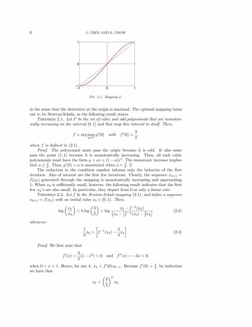
on the real line. Without loss of generality, we assume that ρ(A) = 1 and consideronly the interval x ∈ [−1, 1]. Figure 2.1 plots f .

Because f is odd, we further restrict our attention to the interval [0, 1]. Themapping f on [0, 1] is monotonically increasing and admits x < f(x), except whenx = 0 or 1. Hence, one intuitive explanation of why the iteration Xk+1 = f(Xk)converges to the sign of A is that f pushes all the positive eigenvalues of A toward 1 in amonotonic manner (and similarly pushes the negative eigenvalues toward −1). Amongall these eigenvalues, the one that converges the most slowly is the eigenvalue closestto the origin. Let this eigenvalue be x0, and without loss of generality assume thatx0 > 0. Then, the initial iteration reduces the condition number from 1/x0 to 1/f(x0).When A is ill-conditioned (i.e., x0 ≈ 0), the rate of reduction is f(x0)/x0 ≈ f ′(0).Because of the significance of f ′(0), one naturally asks what is the optimal mapping


−1 0 1−1

0

1

Fig. 2.1. Mapping f .

in the sense that the derivative at the origin is maximal. The optimal mapping turnsout to be Newton-Schulz, as the following result states.

Theorem 2.1. Let P be the set of cubic and odd polynomials that are monoton-ically increasing on the interval [0, 1] and that map this interval to itself. Then,

f = arg maxg∈P

g′(0) with f ′(0) =3

2,

where f is defined in (2.1).Proof. The polynomial must pass the origin because it is odd. It also must

pass the point (1, 1) because it is monotonically increasing. Then, all such cubicpolynomials must have the form g = ax+ (1− a)x3. The monotonic increase impliesthat a ≤ 3

2 . Thus, g′(0) = a is maximized when a = 32 .

The reduction in the condition number informs only the behavior of the firstiteration. Also of interest are the first few iterations. Clearly, the sequence xk+1 =f(xk) generated through the mapping is monotonically increasing and approaching1. When x0 is sufficiently small, however, the following result indicates that the firstfew xk’s are also small. In particular, they depart from 0 at only a linear rate.

Theorem 2.2. Let f be the Newton-Schulz mapping (2.1), and define a sequencexk+1 = f(xk) with an initial value x0 ∈ (0, 1). Then,

log

(xkx0

)< k log

(3

2

)< log

xk − f−1(xk)13x0 −

[f−1(xk)− 2

3xk] (2.2)

whenever

1

3x0 >

[f−1(xk)− 2

3xk

]. (2.3)

Proof. We first note that

f ′(x) =3

2(1− x2) > 0 and f ′′(x) = −3x < 0,

when 0 < x < 1. Hence, for any k, xk < f ′(0)xk−1. Because f ′(0) = 32 , by induction

we have that

xk <

(3

2

)k

x0.


This proves the first inequality of (2.2).

Next, we have

(3

2

)k

x0 − xk =

(3

2

)k−1(3

2x0 − x1

)+

(3

2

)k−2(3

2x1 − x2

)+ · · ·+

(3

2

)0(3

2xk−1 − xk

).

Because f ′(0) = 32 and f ′ is decreasing, we have that 3

2x − f(x) is positive and isincreasing. Then,(

3

2

)k

x0 − xk <

[(3

2

)k−1

+ · · ·+(

3

2

)0](

3

2xk−1 − xk

)

=

(32

)k − 132 − 1

(3

2f−1(xk)− xk

).

Rearranging terms, we obtain{(3

2− 1

)x0 −

(3

2f−1(xk)− xk

)}(3

2

)k

<3

2

[xk − f−1(xk)

],

which proves the second inequality of (2.2).

To explain the use of Theorem 2.2, we give an example. Consider that thebound (2.2) is with respect to k. Table 2.1 gives the numeric values of (2.2) forx0 = 10−3, where NA means the condition (2.3) is invalid. One sees that the boundapplies only when xk is not close to 1 (otherwise (2.3) is invalid); however, wheneverit is applicable, the bound for integer k is tight. Thus, we interpret the inequality onthe left as

log

(xkx0

)≈ k log

(3

2

)(2.4)

for small xk. In other words, xk grows linearly for the first few k’s when the startingvalue x0 is sufficiently small. Note that the factor log

(32

)is important; we will return

to this factor later.

We summarize a few facts in the following theorem, which connects the scalariteration with the matrix iteration. The validity is clear based on the precedingdiscussions; hence, the proof is omitted.

Theorem 2.3. For a Hermitian matrix A and the Newton-Schulz mapping fdefined in (2.1), consider the matrix iteration Xk+1 = f(Xk), X0 = A, and thescalar iteration xk+1 = f(xk). If the spectral radius of A is 1 and x0 is the smallestmagnitude eigenvalue of A, then we have the following.

1. xk is the smallest magnitude eigenvalue of Xk for all k.2. The spectral radius of Xk is 1 for all k; hence the condition number of Xk is

1/xk.3. ‖Xk − S‖2 = |xk − 1| for all k.4. xk → 1 monotonically, and hence ‖Xk − S‖2 → 0 monotonically.


Table 2.1Numerical values of (2.2) for x0 = 10−3.

k 1 2 3

Bound (2.2) 0.99.. < k < 1.00.. 1.99.. < k < 2.00.. 2.99.. < k < 3.00..xk 1.5000e-03 2.2500e-03 3.3750e-03

k 4 5 6

Bound (2.2) 3.99.. < k < 4.00.. 4.99.. < k < 5.00.. 5.99.. < k < 6.00..xk 5.0625e-03 7.5936e-03 1.1390e-02

k 7 8 9

Bound (2.2) 6.99.. < k < 7.00.. 7.99.. < k < 8.01.. 8.99.. < k < 9.03..xk 1.7085e-02 2.5624e-02 3.8428e-02

k 10 11 12

Bound (2.2) 9.99.. < k < 10.13.. 10.99.. < k < 11.51.. 11.98.. < k < 14.51..xk 5.7614e-02 8.6325e-02 1.2917e-01

k 13 14 15

Bound (2.2) 12.97.. < k < NA 13.94.. < k < NA 14.87.. < k < NA

xk 1.9267e-01 2.8543e-01 4.1652e-01

3. Scaled Newton-Schulz (step 1). In this section, we derive a variant ofNewton-Schulz so that the iteration progresses better initially. The optimal variantturns out to be a simple scaling of the Newton-Schulz iterates.

Theorem 2.1 states that the Newton-Schulz mapping f is optimal among all cubicand odd polynomials that map [0, 1] to [0, 1], if in addition the polynomial is requiredto be increasing. To obtain a polynomial whose derivative at the origin is even larger,we need to sacrifice the monotonicity. Define

P ′ = {cubic and odd polynomial g : g([0, 1]) = [0, 1]}.

The polynomials in P ′ can be parameterized in several ways. Consider g(x) = ax+bx3,where a > 0. We crop g in the box [0, c]× [0, d] and normalize it to obtain

g(x) =1

dg(cx) =

ac

dx+

bc3

dx3. (3.1)

When d is the maximum of g on [0, c], such polynomials g constitute the set P ′.One can separate the values of b and c into three cases and calculate that

d =

ac+ bc3, in case 1: b ≥ 0

ac+ bc3, in case 2: b < 0 and c ≤√− a

3b

2a

3

√− a

3b, in case 3: b < 0 and c >

√− a

3b.

(3.2)

See Figure 3.1 for visual examples of the three cases.In case 1, for all x ∈ [0, 1], g(x) ≤ x; in case 2,

g′(0) =ac

d=

ac

ac+ bc3≤ 3

2,

because c ≤√− a

3b . These two cases do not yield a better polynomial than the


0 c0

d

(a) Case 1, a = 1, b = 0.1

0 c0

d

(b) Case 2, a = 1, b = −0.012

0 c0

d

(c) Case 3, a = 1, b = −0.03

Fig. 3.1. Function g in different cases of (3.2). c = 5.

standard Newton-Schulz mapping f does. On the other hand, in case 3,

g′(0) =ac

d=

3

2c

/√− a

3b,

which is larger than 32 . Hence, we further explore this case.

Let α = c/√− a

3b , which is greater than 1. The polynomial in case 3 is simplifiedto

g(x) =3

2αx− 1

2α3x3. (3.3)

Such a polynomial passes the origin, monotonically increases to the maximum 1, andthen decreases until touching x = 1. When α becomes larger, the derivative at theorigin is steeper, the x value that achieves maximum moves toward the left, and g(1)gets closer to 0. In the extreme case, we solve g(1) = 0 and obtain that α =

√3.

Hence, the valid range of α is between 1 and√

3.As before, we let x0 > 0 be the smallest magnitude eigenvalue, whereas the

largest is 1. We want α to be optimal in the sense that after the mapping g, thecondition number of the matrix is maximally reduced. Such an α is obtained bysolving g(x0) = g(1); see Figure 3.2. The solution gives

α =

√3

1 + x0 + x20

. (3.4)

Because such an α yields a mapping g that maps the interval [x0, 1] to [g(x0), 1], thesmallest magnitude eigenvalue of the matrix is g(x0) after mapping.

Thus, we apply the optimal mapping g iteratively on the matrix. Note that gkeeps changing because the smallest magnitude eigenvalue does so, too. We start withan initial matrix X0 = A/λ|max | such that the spectral radius of X0 is 1. Then, itssmallest magnitude eigenvalue x0 = λ|min |/λ|max |. The iteration maintains a loopinvariant such that the smallest magnitude eigenvalue of Xk is xk. Specifically, theiteration reads

Xk+1 =1

2αkXk(3I − α2

kX2k), (3.5a)

where

αk =

√3

1 + xk + x2k

and xk+1 =1

2αkxk(3− α2

kx2k). (3.5b)


0 x0 10

1

Fig. 3.2. Optimal mapping g given x0.

We call (3.5) the optimally scaled Newton-Schulz iteration.

3.1. Analysis. The optimal mapping g in the preceding discussion depends onthe smallest magnitude eigenvalue. We may write an eigenvalue-independent mappingto characterize the scaled iteration instead:

h(x) =3

2αx− 1

2α3x3, where α(x) =

√3

1 + |x|+ x2. (3.6)

Figure 3.3 plots h on [−1, 1], together with the standard Newton-Schulz mapping ffor comparison.

−1 0 1−1

0

1

h: scaled NSf: standard NS

Fig. 3.3. Mapping h (scaled Newton-Schulz) and f (Newton-Schulz).

We note that different from the case of f , we shall not treat h as a matrixfunction and write Xk+1 = h(Xk), because α takes only a scalar value x as input.By construction, the smallest magnitude eigenvalue maintains its “smallest” propertyafter one iteration. Hence, we define the matrix counterpart of h as

h(X) =3

2αX − 1

2α3X3, where α(X) =

√3

1 + λ|min |(X) + λ|min |(X)2. (3.7)

Then, the iteration Xk+1 = h(Xk) is consistent with that of (3.5).Clearly, the mapping h is monotonically increasing on [0, 1], and it maps this

interval to itself. Because α ≥ 1, we always have h(x) ≥ f(x) for x ∈ (0, 1). Hence,for the same initial value x0 = x0 ∈ (0, 1), the sequence xk+1 = h(xk) is always largerthan the sequence xk+1 = f(xk), elementwise. Because xk → 1 and xk is boundedby 1, the sequence xk monotonically increases to the limit 1, the same as does the


sequence xk. Furthermore, xk is always closer to the limit than is xk. We summarizethis result, together with other facts in the following theorem, whose proof is clearbased on the foregoing discussion. This theorem connects the matrix iteration withthe scalar iteration. One should compare this result with Theorem 2.3.

Theorem 3.1. For a Hermitian matrix A and the optimally scaled Newton-Schulz mappings h and h defined in (3.6) and (3.7), respectively, consider the matrixiteration Xk+1 = h(Xk), X0 = A, and the scalar iteration xk+1 = h(xk). If thespectral radius of A is 1 and x0 is the smallest magnitude eigenvalue of A, then wehave the following.

1. xk is the smallest magnitude eigenvalue of Xk for all k.2. ‖Xk − S‖2 = |xk − 1| for all k.3. xk → 1 monotonically, and hence ‖Xk − S‖2 → 0 monotonically.4. The spectral radius of Xk converges to 1.

Furthermore, for the iteration xk+1 = f(xk) where x0 = x0 and where f is thestandard Newton-Schulz mapping (2.1), we have xk < xk for all k > 0.

The significance of the first conclusion of Theorem 3.1 is that the convergencebehavior of Xk is completely characterized by that of xk. Then, we need to focuson only the mapping h. The following theorem states the limiting and the initialbehavior of the scaled iterations.

Theorem 3.2. Let h be the mapping of the optimally scaled Newton-Schulziteration (3.6), and define a sequence xk+1 = h(xk) with an initial value x0 ∈ (0, 1).Then

1. xk converges to 1 quadratically; and2. we have

log

(xkx0

)< k log

(3

2

√3

)< log

xk − h−1(xk)(1− 2

3√

3

)x0 −

[h−1(xk)− 2

3√

3xk

] (3.8)

whenever (1− 2

3√

3

)x0 >

[h−1(xk)− 2

3√

3xk

].

Proof. We already know that xk converges to 1 in Theorem 3.1. Because h(x)−1 =− 1

2 (αx+ 2)(αx− 1)2, we have

limx→1

|h(x)− 1||x− 1|2

=

(limx→1

|αx+ 2|2

)(limx→1

αx− 1

x− 1

)2

=3

2

(limx→1

dα

dx+ α

)2

=3

8, (3.9)

where the second equality follows from L’Hospital’s rule. This shows that the conver-gence is quadratic.

The result (3.8) is proved by using the same technique as that for proving (2.2)in Theorem 2.2. To save space, we omit the details here.

Similar to the interpretation of Theorem 2.2, we see that the bound (3.8) is tight.For example, when x0 = 10−3, the numeric values of the bound are given in Table 3.1.Hence, we write

log

(xkx0

)≈ k log

(3

2

√3

). (3.10)


Compare (3.10) with (2.4), which we repeat here by adding a tilde to denote thesequence generated through the f mapping (as we previously did):

log

(xkx0

)≈ k log

(3

2

).

Because the ratio between log(

32

√3)

and log(

32

)is 2.35.., we can loosely conclude

that

x2k < xk < x3k.

This means that initially (when k is small), the optimally scaled Newton-Schulz itera-tion increases the iterate xk at least twice as fast as does the standard Newton-Schulziteration.

Table 3.1Numerical values of (3.8) for x0 = 10−3.

k 1 2 3

Bound (3.8) 0.99.. < k < 1.00.. 1.99.. < k < 2.00.. 2.99.. < k < 3.03..xk 2.5968e-03 6.7378e-03 1.7445e-02

k 4 5 6

Bound (3.8) 3.98.. < k < 4.28.. 4.95.. < k < NA 5.88.. < k < NA

xk 4.4914e-02 1.1383e-01 2.7539e-01

On closing this section, we remark that in the convergence guarantee of (3.5), x0

need not be the smallest magnitude eigenvalue of X0. The following theorem statesthat (3.5) always converges no matter what value x0 takes. More amazing is that thequadratic rate of convergence is also maintained. Hence, the price paid for using anarbitrary x0 is only some more iterations.

Theorem 3.3. For the optimally scaled Newton-Schulz iteration (3.5), Xk con-verges to S quadratically for any x0 ∈ (0, 1).

Proof. We repeat (3.5) in the following for better reading:

Xk+1 =1

2αkXk(3I − α2

kX2k). (3.11)

Because the sequence xk is computed through the fixed-point mapping xk+1 = h(xk),for any x0 ∈ (0, 1), xk converges to 1 quadratically. Hence, αk also converges to 1quadratically. We use an auxiliary sequence

Yk+1 =1

2Yk(3I − Y 2

k ), Y0 = X0 (3.12)

to gauge the convergence behavior of Xk. Clearly, the sequence Yk results from thestandard Newton-Schulz iteration, and it converges to S quadratically.

Let Vk = Xk − Yk, Wk = Yk − S, and εk = |αk − 1|. We have

‖αkXk − Yk‖2 ≤ ‖αkXk − αkYk‖2 + ‖αkYk − Yk‖2= αk‖Vk‖2 + εk‖Yk‖2 ≤ (1 + εk)‖Vk‖2 + εk(1 + ‖Wk‖2). (3.13)


We further let Zk = αkXk − Yk. By noting that Xk and Yk commute (because bothare polynomials of X0), we subtract (3.12) from (3.11) and obtain

‖Vk+1‖2 =1

2‖Zk(3I − Z2

k − 3αkXkYk)‖2

≤ 1

2‖Zk‖2

(3‖I − Y 2

k ‖2 + ‖Zk‖22 + 3‖Zk‖2‖Yk‖2)

≤ 1

2‖Zk‖2

(‖Zk‖22 + 3(1 + ‖Wk‖2)‖Zk‖2 + 3(2‖Wk‖2 + ‖Wk‖22)

).

With the help of (3.13) we further expand the inequality of ‖Vk+1‖2 and obtain

‖Vk+1‖2 ≤[3(εk + ‖Wk‖2) +O(ε2k + εk‖Wk‖2 + ‖Wk‖22)

]· ‖Vk‖2

+O(ε2k + εk‖Wk‖2 + ‖Wk‖22 + ‖Vk‖22).

Note that both εk and ‖Wk‖2 converge to 0 quadratically. Because ‖V0‖2 = 0, by in-duction we have that ‖Vk‖2 = O(εk+‖Wk‖2). This means that the difference betweenXk and Yk converges to 0 quadratically. Thus, Xk converges to S quadratically.

4. Scaled Newton-Schulz (step 2), stable version. Unfortunately, the op-timal scaling (3.5) is numerically unstable at convergence. Stability is measured bythe backward error

‖A−Xk(H +H∗)/2‖‖A‖

(4.1)

of the polar decomposition of A, where H is the Hermitian polar factor X∗kA and‖ · ‖ is any subordinate matrix norm. The curve annotated as “scaled Newton-Schulz,unstable” in Figure 1.1 shows that the iteration (3.5) cannot decrease the backwarderror to the level of machine precision. The instability stems from the subtle fact thatrepeated matrix-matrix multiplications may alter the eigenspace of a matrix. Thus,an alternative stability measure is

‖AXk −XkA‖‖A‖‖Xk‖

,

which measures how well Xk commutes with A. This measure leads to the sameinstability conclusion for (3.5).

A simple but robust fix returns to the derivation of the optimal mapping g in (3.3)and (3.4). Recall that x0 denotes the smallest magnitude eigenvalue. The optimalscaling factor α is derived by equating g(x0) with g(1). When x0 is small, so isg(x0). Then, such an α forces the largest magnitude eigenvalue 1 to drop to g(1), asubstantial decrease. In the analysis of [22], such a decrease is the origin of instability.To circumvent the issue, we set a threshold t that limits the smallest value of g(1).Equating g(1) = t gives

3

2α− 1

2α3 − t = 0. (4.2)

Clearly, α is a decreasing function of t when α > 1. Let α solve (4.2), which has onlyone root on the interval (1,

√3). Then, the modified scaling factor α reads

α = min

{√3

1 + x0 + x20

, α

}, (4.3)


which is upperbounded by α.An appropriate value of the threshold t cannot be too small or too large. If too

small, the largest magnitude eigenvalue still undergoes a significant decrease. If toolarge, g′(0) = 3

2α decreases accordingly and undermines the acceleration of Newton-Schulz. Let us consider three candidates: 1, 0.1, and 0.01. The first candidate isequivalent to the standard Newton-Schulz—no scaling. The third candidate yieldsa backward error curve that stagnates above the level of machine precision. On theother hand, the second candidate survives all the stability tests we have conducted.Thus, we set t = 0.1.

One additional benefit of using t = 0.1 is that it barely changes the convergenceprogress of the optimally scaled iteration (3.5). Specifically, we write the new mapping

h(x) =3

2αx− 1

2α3x3, where α(x) = min

{√3

1 + |x|+ x2, α

}. (4.4)

Comparing h with h in (3.6), the curve of h is visually indistinguishable from that ofh (plotted in Figure 3.3). Moreover, an analogous result to (3.10) is

log

(xkx0

)≈ k log

(3

2α

),

where {xk} denotes the sequence generated by the h mapping. Here, α = 1.69... whent = 0.1, which makes log

(32 α)/ log

(32

)= 2.30.... Such a ratio is sufficiently close

to the ratio log(

32

√3)/ log

(32

), leading to an almost identical convergence progress

compared with the optimally scaled Newton-Schulz.We summarize the whole computational procedure in Algorithm 1. This algorithm

is numerically stable.

Algorithm 1 A Stable, Scaled Newton-Schulz Method for Computing sign(A)

1: Compute λ|min | and λ|max | of A2: Let X0 = A/λ|max | and x0 = λ|min |/λ|max |.

3: Solve 12 α(3− α2) = t for α, where t = 0.1.

4: for k = 0, 1, . . .maxiter do

5: Compute αk = min

{√3

1 + xk + x2k

, α

}.

6: Update Xk+1 = 12αkXk(3I − α2

kX2k).

7: Symmetrize Xk+1 ← 12 (Xk+1 +X∗k+1) if required.

8: Update xk+1 = 12αkxk(3− α2

kx2k).

9: If converged, exit loop.10: end for11: return Xk+1

4.1. Computational costs. We list in Table 4.1 the maximum number of it-erations needed for the backward error (4.1) to reach 10−16 for different values ofthe matrix condition number. Four stable iterations are compared: the standardNewton-Schulz; the stable, scaled Newton-Schulz (Algorithm 1); Newton with Byers-Xu scaling; and Halley (DWH) with the QR implementation (1.3). One clearly sees


that Algorithm 1 converges approximately twice as fast as the standard Newton-Schulz, whereas it requires only a few more times of iterations compared with the lasttwo methods.

Table 4.1Iteration counts for various iterations to converge to 10−16.

Condition number 102 104 106 108 1010 1012 1014 1016

Newton-Schulz (NS) 17 28 39 51 62 74 85 96Stable, scaled NS 10 15 19 24 29 34 39 44Newton, Byers-Xu 6 7 7 8 8 8 9 9

Halley, DWH with QR 4 5 5 5 5 5 6 6

In terms of flop count, Newton-Schulz and scaled Newton-Schulz require 2n3 flopsper iteration in the Hermitian case (neglecting lower-order terms). Scaled Newtonalso requires 2n3 flops per iteration if the inversion is computed by using a triangularfactorization, or 6n3 flops if the inversion is computed by using a backward stablebidiagonal reduction-based algorithm [21]. The dynamically weighted Halley iterationimplemented using QR factorization requires (26/3)n3 flops per iteration, or (16/3)n3

flops per iteration if implemented carefully with Givens rotations.In terms of communication volume in a parallel implementation, although matrix

multiplication, Cholesky, and QR factorization have asymptotically the same lowerbounds, current practical “communication-avoiding” implementations of Choleskyand QR come only within a factor of log p, where p is the number of processors,and may perform many more flops than the standard algorithms in order to attainreduced communication [1, 5]. On the other hand, matrix multiplication attains itscommunication lower bound with standard Cannon and SUMMA algorithms, andmany optimized implementations exist for different computer platforms.

In summary, the main computational difference between the Newton-Schulz al-gorithms (including Algorithm 1) and Newton and Halley is matrix inversion (orfactorizations used for reformulating inversion). With inversion, much faster conver-gence may be attained, but it comes at the cost of potentially poorer scalability. Thisis a classic tradeoff. The best algorithm to use in any situation will likely depend onthe computer architecture, the number of available processors, the problem size, andthe matrix condition number.

5. Practical implementation. A few implementation issues for Algorithm 1are addressed in this section.

5.1. Stopping criterion. We need a convergence test for line 9 of Algorithm 1.Write Xk − S = (XkS − I)S; then,

‖Xk − S‖ = ‖(XkS − I)S‖ ≤ ‖XkS − I‖‖S‖.

Note that the inequality is an equality in the 2-norm case. When Xk ≈ S, we obtainthe relative error

‖Xk − S‖‖S‖

/ ‖X2k − I‖.

Hence, it is straightforward to use ‖X2k − I‖ ≤ tol as the convergence criterion,

where tol is the relative tolerance. Any submultiplicative norm can be used, but for


computational convenience we use the Frobenius norm. The computed squared factorX2

k is stored and used in the next iteration for updating Xk. The best attainableerror is nu/2, where u is the machine precision [11, Section 5.1].

Note that this stopping criterion verifies only the unitarity of Xk but not theeigenspace. At detected convergence, one may in addition compute the backwarderror (4.1) to ensure that the computed Xk is stable. Computing (4.1) requires twoextra matrix-matrix multiplications.

5.2. Shifting. A useful observation is that shifts of A do not change sign(A) aslong as these shifts do not cause eigenvalues of A to cross the origin. Hence, we canperform a shift to precondition A (that is, to start with a larger x0) and to improveconvergence. Specifically, we first compute four eigenvalues of interest:

λ−min(A) ≤ λ−max(A) < 0 < λ+ min(A) ≤ λ+ max(A),

which are the smallest negative, the largest negative, the smallest positive, and thelargest positive eigenvalue of A, respectively, and compute a shift

τ =λ−max(A) + λ+ min(A)

2.

Then, we input A′ = A − τ and run Algorithm 1 to obtain S = sign(A′). The twoeigenvalues in Algorithm 1 now become

λ′|max | = max{|λ+ max(A)− τ |, |λ−min(A)− τ |}λ′|min | = min{|λ−max(A)− τ |, |λ+ min(A)− τ |}.

For the amount of reduction in iterations caused by the reduction in condition number,see Table 4.1.

5.3. Eigenvalue estimation. The requirement of eigenvalue computation inAlgorithm 1 forms several levels of difficulty. Our discussion here is oriented to generaleigenvalue techniques and software support. Whereas small-scale eigenvalue problemshave a standard solution through orthogonal transformations to the condensed form,large-scale eigenvalue problems are challenging, even if only a few extreme and/orinterior eigenvalues are sought. We make no effort to design new eigenvalue techniques;rather, the issue we address here is how practical Algorithm 1 is in a large-scale settingwith off-the-shelf software packages. For a comprehensive treatment of the theoryand state-of-the-art eigenvalue methods, we refer the readers to Saad’s book [25].Practitioners might develop specialized eigenvalue solvers for their applications.

At the easiest level, no eigenvalue computation is carried out. The largest mag-nitude eigenvalue can be estimated by using the Gershgorin circle theorem. Thetheorem ensures that the spectral radius of the scaled matrix is no greater than 1. Adrawback of this method is that in some cases the bound provided by the theorem istoo pessimistic. On the other hand, the starting value x0 can be arbitrary, as notedearlier; what is sacrificed is the optimal convergence. If a good estimate of the con-dition number of A is known a priori, the extra number of iterations may not be toolarge. Note that if x0 is not an accurate estimate, shifting is impossible.

At the next level, Gershgorin is replaced by a computation of the largest magni-tude eigenvalue. This eigenvalue can be computed by using the Lanczos algorithm.Accelerated by implicit shifts and restarts [14, 27], the Lanczos algorithm convergesrapidly when the targeted eigenvalue is not clustered with others. The algorithm has


been implemented in ARPACK [15]. The dominant cost of the calculation is formingmatrix-vector products, for which extensive research has been devoted to designinghigh-performance software as well as linear-time or near-linear-time algorithms fordifferent types of matrices, such as sparse, Toeplitz, or kernel matrices. Because thedesired eigenvalue converges from inside the spectrum interval, if this eigenvalue can-not be computed to high accuracy, a correction term must be added to ensure thatthe spectral radius of the scaled matrix is no greater than 1.

The most difficult level comprises the calculation of all four eigenvalues mentionedin Section 5.2. In particular, shifting is useful and produces the correct result onlywhen the two innermost eigenvalues are computed accurately. Computing these eigen-values, however, is a well-known challenge in applications. The Lanczos algorithmdiscussed in the preceding paragraph can be reused, by applying A−1 as the operatorinstead of A. Then, the dominant cost becomes solving linear systems with A. Forsparse matrices, a direct method is the most robust; software includes CHOLMOD [4]and SuperLU [17]. For dense matrices arising from kernels, direct solves with high-accuracy off-diagonal compression techniques are gaining popularity [30]. Iterativesolvers are in general not as robust as direct solvers but sometimes are highly effi-cient with a good preconditioner. To avoid being too restricted by the standard formof Lanczos, we also mention other popular methods for computing interior eigenval-ues: shift-and-invert [7], Davidson’s method [3] and its improvements [20, 9], andpolynomial filtering [8], the details of which are not further discussed.

6. Numerical experiments. In this section we conduct numerical experimentswith matrices from various sources. Many aspects of Algorithm 1 are examined, in-cluding stability, eigenvalue estimates, shifting, and computing environments (includ-ing a single desktop with multithreaded Matlab and a computing cluster with MPI).The goal is to demonstrate the stability and efficiency of the proposed algorithm. Thesymmetrization step (line 7 of Algorithm 1) is enforced.

6.1. Matrices from the Matlab gallery and Higham’s toolbox. We em-pirically verify the numerical stability of Algorithm 1 with applicable matrices fromthe Matlab gallery and Higham’s matrix computation toolbox.1 The size of the matri-ces is set to 20×20. If a matrix A is not Hermitian, we modify it by A← (A+A∗)/2.The condition number of the modified matrices ranges from 1 to 1.1e+19. When thestopping criterion is set to ‖X2

k − I‖F ≤ nu/2, the largest backward error (4.1) is2.3e-15 among all matrices.

6.2. An artificial matrix. We test the effect of inaccurate eigenvalue estimateson the convergence of Algorithm 1. For this, consider a matrix built using the standard2D Laplacian L:

A =

[L− cλ|min |(L)

−2L+ 2cλ|min |(L)

], (6.1)

where c < 1 is a tunable parameter. The eigenvalues of such a matrix are known.When c→ 1, A is increasingly ill-conditioned.

We use a 20 × 30 grid to construct L and test with two choices of c: 1 − 10−4

and 1− 10−8. Table 6.1 lists the number of iterations with different estimates of theeigenvalues λ|max |(A) and λ|min |(A) in Algorithm 1. For the estimated eigenvalues,we let λ|max |(A) be twice the exact value. Usually, this eigenvalue is easy to estimate,

1http://www.maths.manchester.ac.uk/~higham/mctoolbox/


and setting it to be twice as large is sufficiently conservative. On the other hand, forλ|min |(A), we perturb the exact value by a factor of 10 or 100 to simulate highlyinaccurate estimates. In the table, the first row always uses the exact eigenvalues.The column “NS” stands for Newton-Schulz and “sNS” stands for the stable, scaledvariant. As expected, when the eigenvalue estimates are very crude, the number ofiterations significantly increases. Nevertheless, the scaled iteration still requires manyfewer iterations than does standard Newton-Schulz. The largest backward error (4.1)is 1.49e-16 among all matrices.

Table 6.1Number of iterations for matrix A in (6.1). “NS” stands for Newton-Schulz and “sNS” stands

for the proposed method (Algorithm 1). “Est. λ|max |” and “Est. λ|min |” are perturbed eigenvaluesof A, except in the first row, which uses the exact eigenvalues.

c = 1− 10−4, cond = 4.86802e+06 c = 1− 10−8, cond = 4.86802e+10

Est. λ|max | Est. λ|min | NS sNS Est. λ|max | Est. λ|min | NS sNS1: 15.8696 3.26e-06 43 21 15.8696 3.26e-10 66 312: 15.8696 1.00e-06 43 22 15.8696 1.00e-10 66 323: 15.8696 1.00e-04 43 27 15.8696 1.00e-08 66 364: 15.8696 1.00e-08 43 27 15.8696 1.00e-12 66 375: 31.7392 3.26e-06 45 22 31.7392 3.26e-10 68 326: 31.7392 1.00e-06 45 23 31.7392 1.00e-10 68 337: 31.7392 1.00e-04 45 27 31.7392 1.00e-08 68 378: 31.7392 1.00e-08 45 28 31.7392 1.00e-12 68 38

6.3. PARSEC matrices. We test the use of shifting on the PARSEC collectionof matrices arising from density functional theory in quantum mechanics. The ma-trices can be downloaded from the University of Florida Sparse Matrix Collection.2

This collection contains matrices of size ranging from several hundreds to a few hun-dred thousands. The computations are carried out on the Blues computing cluster3

at Argonne National Laboratory. The machine comprises 310 compute nodes, eachof which has 16 Intel Sandy Bridge cores and 64 GB of memory. The compute nodesare connected by QLogic QDR InfiniBand with a fat-tree topology.

We prepared two programs, one in Matlab and the other in C with MPI. TheMatlab program runs on one compute node with a maximum of 16 threads by de-fault. It uses the backslash command for solving linear systems and uses the eigs

command for computing eigenvalues. The C program runs on a large number ofcompute nodes. It uses SuperLU for solving linear systems and uses PARPACK forcomputing eigenvalues. The matrix-matrix multiplication is implemented by usingScaLAPACK.

Preliminary investigation of the spectra shows that the inertias of the matrices arehighly skewed. We thus center the matrices at 1/3 of the spectrum as a preprocessing(that is, the new origin is located at 1

3λ+ max + 23λ−min). The cutoff 1/3 is arbitrary;

our purpose is to demonstrate calculations with an arbitrary change of the origin.

We perform calculations with the preprocessed matrices, once before shifting andonce after shifting. The computed results are listed in Table 6.2. One sees that shiftingdoes help reduce the condition number and the iteration count. The reduction on thematrices benzene and Si34H36 is substantial.

2http://www.cise.ufl.edu/research/sparse/matrices/3http://www.lcrc.anl.gov/about/blues


Table 6.2Computation results of the matrices in the PARSEC collection. The matrices were preprocessed

by centering. Inertia a/b means a positive eigenvalues and b negative eigenvalues. “Cond” is thecondition number. “Iter” is the number of iterations. “B-Err” is the backward error (4.1).

Before Shift After ShiftMatrix n Inertia Cond Iter B-Err Cond Iter B-Err

Si2 769 516/253 2.5e+3 13 4.2e-15 1.3e+3 12 3.8e-15

SiH4 5,041 3,467/1,574 1.4e+4 15 4.7e-15 2.3e+3 13 4.2e-15

benzene 8,219 5,459/2,760 5.4e+6 21 6.6e-15 1.5e+4 15 5.0e-15

Si10H16 17,077 11,575/5,502 3.6e+4 16 5.4e-15 2.5e+4 15 5.4e-15

SiO 33,401 22,620/10,781 3.3e+4 16 8.6e-15 2.3e+4 15 8.5e-15

Ga3As3H12 61,349 61,348/1 2.6e+0 5 6.7e-15 1.1e+0 4 4.4e-16

Si34H36 97,569 65,621/31,948 1.4e+6 20 8.6e-15 6.3e+4 16 7.3e-15

Table 6.3 lists the timings of the calculations for the matrices with optimal shift-ing. Results on the top part of the table are obtained by running the Matlab pro-gram, those in the bottom part by running the C program. As expected, computingthe interior eigenvalues λ−max and λ+ min is more costly than computing the exterioreigenvalues λ−min and λ+ max. Nevertheless, compared with the iterations, the timefor computing the eigenvalues is generally smaller.

Table 6.3Timing results of the computation of the matrices in Table 6.2. All times are in seconds.

Matrix n Parallelism λ−min λ−max λ+min λ+max sNS

Si2 769 16 threads 8.9e-1 5.5e-1 8.6e-1 3.9e-2 6.1e-1

SiH4 5,041 16 threads 9.9e-2 2.8e+1 5.7e+1 9.0e-2 8.8e+1

benzene 8,219 16 threads 1.8e-1 8.1e+1 5.3e+1 1.6e-1 4.4e+2

Si10H16 17,077 16 threads 6.3e-1 8.1e+2 6.1e+2 5.7e-1 3.4e+3

SiO 33,401 1,024 procs 3.8e+0 8.4e+0 6.7e+0 7.4e-1 2.6e+2

Ga3As3H12 61,349 1,024 procs 5.2e+0 1.3e+2 2.3e+1 2.7e-1 4.5e+2

Si34H36 97,569 2,304 procs 1.2e+1 3.5e+1 6.8e+1 5.3e+0 2.6e+3

7. Application: electronic structure calculation. At every iteration of theHartree-Fock algorithm, also known as the self-consistent field (SCF) iteration, aspectral projector called the density matrix is computed from the Fock matrix, whichis an approximation to the Hamiltonian [28]. The density matrix may be computed inmany ways, the most obvious being through an eigenvalue decomposition of the Fockmatrix. In this section we demonstrate the use of our scaled Newton-Schulz algorithmfor computing the density matrix.

Construction of the Fock matrix is the computationally intensive step in SCFiterations, but it is highly parallel. Computation of the density matrix, however,can be the bottleneck limiting parallel scalability: although the density matrix is notextremely large, it must be efficiently computed by using a large number of processors(which were used earlier to construct the Fock matrix), much like the solution ofsmall coarse-grid problems in parallel multigrid. Algorithms of Newton-Schulz type(called McWeeny purification [19] in the quantum chemistry literature) that are richin matrix-matrix multiplications are thus attractive in the high parallelism setting.

We generated the core-Hamiltonian matrix for two hydrocarbon molecules: agraphene-like molecule, C384H48, and a linear alkane, C418H838. The core-Hamiltonian


Table 7.1Hydrocarbon test problems. The dimension of the core-Hamiltonian matrix is the basis size,

and nocc is the number of occupied orbitals. The value λ|min| is the smallest magnitude eigenvalueof A after it has been scaled to have unit spectral radius.

Basis Size nocc λ|min|Graphene C384H48 5,616 1,176 4.1e-05

Alkane C418H838 10,042 1,673 2.4e-05

describes the kinetic energy and nuclear attraction of electrons, but not electron-electron interactions, and is often used as the initial guess for the Fock matrix inSCF iterations. Since the Fock matrix itself depends on the density matrix, the core-Hamiltonian initial guess corresponds to a zero initial guess for the density matrix.Here, we compute the density matrix corresponding to these core-Hamiltonians. Theelements of the core-Hamiltonian matrices were formed by using the Dunning cc-pVDZ basis set [6] using a standard quantum chemistry code [18]. Table 7.1 showsthe resulting matrix dimension (equal to the number of basis functions) for the twotest problems.

The density matrix is the spectral projector associated with the nocc lowest eigen-values and their corresponding eigenvectors, where nocc is the number of occupiedorbitals, or half the number of electrons assuming closed-shell orbitals. To computethe density matrix via the sign function, we first compute the sign of

A = µI −H,

where H is the core-Hamiltonian in our case and µ, known as the Fermi level, separatesthe occupied eigenvalues from the unoccupied eigenvalues. The Fermi level is oftenknown, especially for problems with a large energy band gap. For our tests, we chosethe Fermi level to lie exactly between the nocc and nocc + 1-st eigenvalue of A, sortedin increasing order. This is optimal for the Newton-Schulz method and the scaledvariant. In practice, such an exact shift is not known. On the other hand, using thecore-Hamiltonian is a kind of worse case, since there is no gap of eigenvalues aroundµ, as would be the case for more converged Fock matrices in later SCF iterations. Wenote that once sign(A) is computed, the density matrix is given by (sign(A) + I)/2.The density matrix can also be computed directly from A by using the McWeenymapping g(x) = 3x2 − 2x3, which can also be modified to accelerate convergence aswe have in this paper modified the Newton-Schulz mapping.

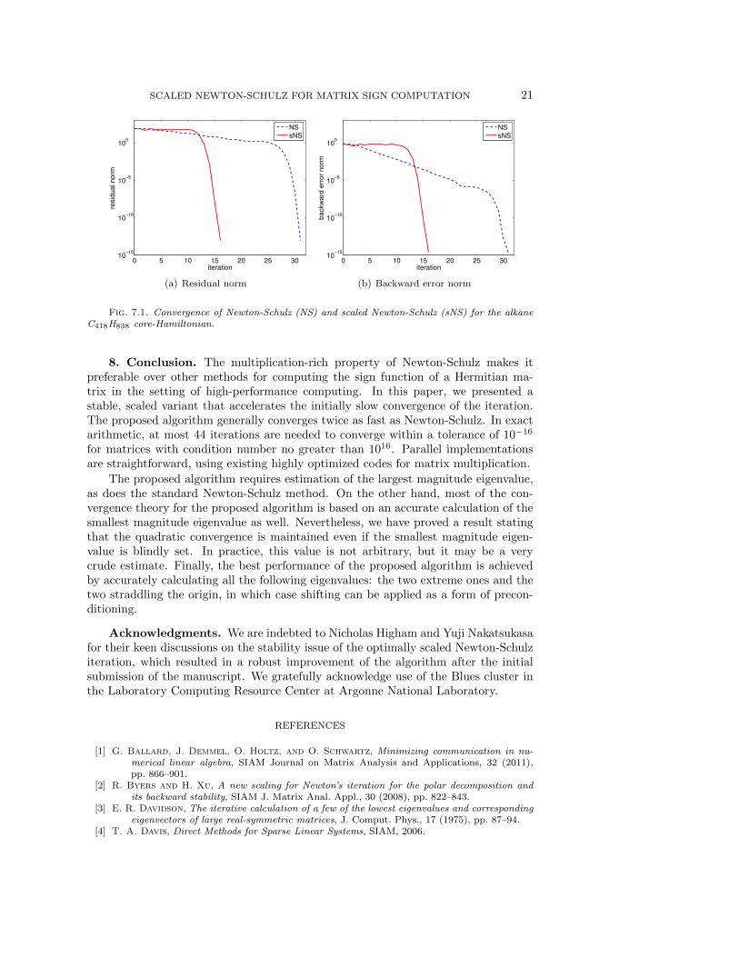
Figure 7.1 plots the residual norm ‖X2k − I‖F and the backward error (4.1) us-

ing the Frobenius norm for Newton-Schulz and for the new scaled method for thealkane test problem. The plots for the graphene test problem are qualitatively thesame. (Note that for Newton-Schultz, an initial scaling of the test matrix is used suchthat the maximum magnitude eigenvalue has magnitude 1.) As we have seen, thescaled method converges in approximately half the number of iterations of the origi-nal method. For the original method, convergence in the Frobenius norm is monotone,as every eigenvalue is improved (pushed toward the correct direction) at each itera-tion. For the scaled method, although it is faster, the situation is different. Here, weobserve a “dip” in the first five iterations: an initial decrease, faster than the decreaseof standard Newton-Schulz, followed by an increase. In the scaled method, only theeigenvalue closest to zero is guaranteed to improve monotonically; the nonmonotoneconvergence of other eigenvalues makes the Frobenius norm of the residual convergenonmonotonically.


0 5 10 15 20 25 3010

−15

10−10

10−5

100

iteration

resid

ua

l n

orm

NS

sNS

(a) Residual norm

0 5 10 15 20 25 3010

−15

10−10

10−5

100

iteration

ba

ckw

ard

err

or

no

rm

NS

sNS

(b) Backward error norm

Fig. 7.1. Convergence of Newton-Schulz (NS) and scaled Newton-Schulz (sNS) for the alkaneC418H838 core-Hamiltonian.

8. Conclusion. The multiplication-rich property of Newton-Schulz makes itpreferable over other methods for computing the sign function of a Hermitian ma-trix in the setting of high-performance computing. In this paper, we presented astable, scaled variant that accelerates the initially slow convergence of the iteration.The proposed algorithm generally converges twice as fast as Newton-Schulz. In exactarithmetic, at most 44 iterations are needed to converge within a tolerance of 10−16

for matrices with condition number no greater than 1016. Parallel implementationsare straightforward, using existing highly optimized codes for matrix multiplication.

The proposed algorithm requires estimation of the largest magnitude eigenvalue,as does the standard Newton-Schulz method. On the other hand, most of the con-vergence theory for the proposed algorithm is based on an accurate calculation of thesmallest magnitude eigenvalue as well. Nevertheless, we have proved a result statingthat the quadratic convergence is maintained even if the smallest magnitude eigen-value is blindly set. In practice, this value is not arbitrary, but it may be a verycrude estimate. Finally, the best performance of the proposed algorithm is achievedby accurately calculating all the following eigenvalues: the two extreme ones and thetwo straddling the origin, in which case shifting can be applied as a form of precon-ditioning.

Acknowledgments. We are indebted to Nicholas Higham and Yuji Nakatsukasafor their keen discussions on the stability issue of the optimally scaled Newton-Schulziteration, which resulted in a robust improvement of the algorithm after the initialsubmission of the manuscript. We gratefully acknowledge use of the Blues cluster inthe Laboratory Computing Resource Center at Argonne National Laboratory.

REFERENCES

[1] G. Ballard, J. Demmel, O. Holtz, and O. Schwartz, Minimizing communication in nu-merical linear algebra, SIAM Journal on Matrix Analysis and Applications, 32 (2011),pp. 866–901.

[2] R. Byers and H. Xu, A new scaling for Newton’s iteration for the polar decomposition andits backward stability, SIAM J. Matrix Anal. Appl., 30 (2008), pp. 822–843.

[3] E. R. Davidson, The iterative calculation of a few of the lowest eigenvalues and correspondingeigenvectors of large real-symmetric matrices, J. Comput. Phys., 17 (1975), pp. 87–94.

[4] T. A. Davis, Direct Methods for Sparse Linear Systems, SIAM, 2006.


[5] J. Demmel, L. Grigori, M. Hoemmen, and J. Langou, Communication-optimal parallel andsequential QR and LU factorizations, SIAM Journal on Scientific Computing, 34 (2012),pp. A206–A239.

[6] T. H. Dunning Jr, Gaussian basis sets for use in correlated molecular calculations. I. Theatoms boron through neon and hydrogen, The Journal of Chemical Physics, 90 (1989),p. 1007.

[7] T. Ericsson and A. Ruhe, The spectral transformation Lanczos method for the numerical so-lution of large sparse generalized symmetric eigenvalue problems, Math. Comp., 35 (1980),pp. 1251–1268.

[8] H.-R. Fang and Y. Saad, A filtered Lanczos procedure for extreme and interior eigenvalueproblems, SIAM J. Sci. Comput., 34 (2012), pp. A2220–A2246.

[9] D. R. Fokkema, G. L. G. Sleijpen, and H. A. V. der, Jacobi–Davidson style QR and QZalgorithms for the reduction of matrix pencils, SIAM J. Sci. Comput., 20 (1998), pp. 94–125.

[10] A. Frommer, T. Lippert, B. Medeke, and K. Schilling, eds., Numerical Challenges inLattice Quantum Chromodynamics, vol. 15 of Lecture Notes in Computational Scienceand Engineering, Springer, 2000.

[11] N. J. Higham, Functions of Matrices: Theory and Computation, SIAM, 2008.[12] C. S. Kenney and A. J. Laub, The matrix sign function, IEEE Transactions on Automatic

Control, 40 (1995), pp. 1330–1348.[13] A. Kie lbasinski and K. Zietak, Numerical behaviour of Higham’s scaled method for polar

decomposition, Numerical Algorithms, 32 (2003), pp. 105–140.[14] R. B. Lehoucq and D. C. Sorensen, Deflation techniques for an implicitly re-started Arnoldi

iteration, SIAM J. Matrix Anal. Appl., 17 (1996), pp. 789–821.[15] R. B. Lehoucq, D. C. Sorensen, and C. Yang, ARPACK Users’ Guide: Solution of Large-

Scale Eigenvalue Problems with Implicitly Restarted Arnoldi Methods, SIAM, 1998.[16] X.-P. Li, R. W. Nunes, and D. Vanderbilt, Density-matrix electronic-structure method with

linear system-size scaling, Phys. Rev. B, 47 (1993), pp. 10891–10894.[17] X. S. Li, An overview of SuperLU: Algorithms, implementation, and user interface, ACM

Trans. Math. Softw., 31 (2005), pp. 302–325.[18] V. Lotrich, N. Flocke, M. Ponton, A. Yau, A. Perera, E. Deumens, and R. Bartlett,

Parallel implementation of electronic structure energy, gradient, and Hessian calculations,The Journal of Chemical Physics, 128 (2008), p. 194104.

[19] R. McWeeny, Some recent advances in density matrix theory, Rev. Mod. Phys., 32 (1960),pp. 335–369.

[20] R. B. Morgan and D. S. Scott, Generalizations of Davidson’s method for computing eigen-values of sparse symmetric matrices, SIAM J. Sci. Stat. Comput., 7 (1986), pp. 817–825.

[21] Y. Nakatsukasa, Z. Bai, and F. Gygi, Optimizing Halley’s iteration for computing the matrixpolar decomposition, SIAM J. Matrix Anal. Appl., 31 (2010), pp. 2700–2720.

[22] Y. Nakatsukasa and N. J. Higham, Backward stability of iterations for computing the polardecomposition, SIAM J. Matrix Anal. Appl., 33 (2012), pp. 460–479.

[23] H. Neuberger, Exactly massless quarks on the lattice, Physics Letters B, 417 (1998), pp. 141–144.

[24] E. H. Rubensson, Nonmonotonic recursive polynomial expansions for linear scaling calculationof the density matrix, J. Chem. Theory Comput., 7 (2011), pp. 1233–1236.

[25] Y. Saad, Numerical Methods for Large Eigenvalue Problems, Revised Edition, SIAM, 2011.[26] Y. Saad, J. Chelikowsky, and S. Shontz, Numerical methods for electronic structure calcu-

lations of materials, SIAM Review, 52 (2010), pp. 3–54.[27] D. C. Sorensen, Implicit application of polynomial filters in a k-step Arnoldi method, SIAM

J. Matrix Anal. Appl., 13 (1992), pp. 357–385.[28] A. Szabo and N. S. Ostlund, Modern Quantum Chemistry: Introduction to Advanced Elec-

tronic Structure Theory, Dover, 1989.[29] J. van den Eshof, A. Frommer, T. Lippert, K. Schilling, and H. A. van der Vorst,

Numerical methods for the QCD overlap operator: I. sign-function and error bounds,Computer Physics Communications, 146 (2002), pp. 203–224.

[30] S. Wang, X. S. Li, J. Xia, Y. Situ, and M. V. D. Hoop, Efficient scalable algorithms forsolving linear systems with hierarchically semiseparable structures. submitted to SIAM J.Sci. Comput., 2012.


The submitted manuscript has been created by UChicago Argonne,LLC, Operator of Argonne National Laboratory (“Argonne”). Ar-gonne, a U.S. Department of Energy Office of Science laboratory,is operated under Contract No. DE-AC02-06CH11357. The U.S.Government retains for itself, and others acting on its behalf, apaid-up nonexclusive, irrevocable worldwide license in said arti-cle to reproduce, prepare derivative works, distribute copies to thepublic, and perform publicly and display publicly, by or on behalfof the Government.

a stable scaling of newton-schulz for improving … · scaled newton-schulz for matrix sign...

Documents