Kybernetika

Ivan M. Havel; Ivan KramosilA stochastic approach to robot plan formation

Kybernetika, Vol. 14 (1978), No. 3, (143)--173

Persistent URL: http://dml.cz/dmlcz/125408

Terms of use:© Institute of Information Theory and Automation AS CR, 1978

Institute of Mathematics of the Academy of Sciences of the Czech Republic provides access to digitizeddocuments strictly for personal use. Each copy of any part of this document must contain theseTerms of use.

This paper has been digitized, optimized for electronic delivery and stamped withdigital signature within the project DML-CZ: The Czech Digital Mathematics Libraryhttp://project.dml.cz

K Y B E R N E T I K A — V O L U M E 14 (1978), NUMBER 3

A Stochastic Approach to Robot Pian Formation

IVAN M. HAVEL, IVAN KRAMOSIL

A new approach to robot plan formation is suggested and discussed, based on probabilistic ideas. The concept of incidental phenomena from [18] is extended into a randomized form and then it is used as a background for exploring approximate plans (plans with a certain degree of execution reliability and of fittnes to a given task). This makes it possible to develop plans with loops, which would otherwise require infinitistic tools.

1. INTRODUCTION

Complexity, in all its various appearances, is one of the nightmares of workers in artificial intelligence and cognitive robotics. It is a common belief that heuristic approaches, combined with strong constraints on the relevant problem domain, are the only available efficient tools for developing systems of intelligent performance. The aim of the present paper is to develop and discuss a novel approach for the area of robot plan formation, based on probabilistic ideas, which is a potential alternative to the heuristic approach. In addition, this technique enables us to introduce certain constructs (loops in plans) that are hard to handle by conventional tools. It must be confessed that the paper contains more definitions than theorems and is more of a con­templative, than of a persuasive character.

Interestingly enough, the previous work in robot plan formation only seldom utilizes probabilistic and descision-theoretic means. Of course, many authors are aware of the possibility but they do not explore it in detail (cf., e.g., [14], [4], [7], [16]). Robot planning is viewed as a decision-making activity in papers [9], [3], [1], [5]. A rather natural idea of branching plans with probabilistically evaluated bran­ches was suggested in [4] and [15], and led to the study of truncated plans in [ l l ] and [12]. In [10] an emphasis was placed on the random character of environment. The advantages of unprecise plans are pointed out in [6]. (Most of the papers men-

tioned above are either suggestive or experimentally oriented, e.g., [1]). The past approaches as well as some future possibilities of stochastic robot decision making are outlined in [8].

The approach suggested in the present paper is characterized by its attention to one aspect of robot planning: on the basis of randomized representation of the changes of environment induced by the robot's actions the planning subsystem of the robot generates approximate plans with a controlled level of reliability as well as of suitability (fittness for the original problem). Our formal framework is logically oriented. It is built on the concept of an image space with branching plans [17] extended by the idea of incidental phenomena [18], the relevant formalism is surveyed in Section 2. In Section 3 the idea of incidental phenomena is extended into a ran­domized form and the first of our variants of stochastic plans, the so called (e, <5)-stochastic plan, is defined. Motivation and formalism for incorporating (potentially infinite) loops into plans and representing them by a special symbol (Kleene star) is the topic of Section 4, where the main concepts of a stochastic star plan and of an e-stochastic star plan are introduced. These concepts enable to work with plans similar as in [17] but infinite due to unbounded loops and thus intractable in the framework of classical logic. In Section 5 two performance measures (the reliability and the suitability) are investigated asymptotically, in their dependence on the num­ber of times a loop is executed. In the last Section 6 some ideas for general algorithmic means for producing cycles are presented.

The new concepts in this paper are mostly introduced in a flexible way covering a variety of possible alternatives. Great care is given to elucidating all notions by informal discussion and by including illustrative examples.

2. IMAGE SPACE WITH INCIDENTAL PHENOMENA: THE DETERMINISTIC CASE

In this section we briefly review the basic concepts of the logical theory of robot problem solving in its original deterministic setting. Our presentation is self-contained but a reader familiar with the approach of [17] and [18] might find it much easier to see the proper intuitive background behind our formalism. We start with some preliminaries.

Since we shall very frequently work with finite sequences of elements of a given set it will be advantageous to adopt certain notational conventions common in formal language theory. Let 3 be a set of abstract symbols. A finite sequence (xlt x2, . . . , x„) of elements of 3 will be written as a string, x1x2. • -x„; the set of all such strings, including the empty string A (to allow for n = 0), is denoted by 3*. Note that 3 £ 3*. By concatenating two strings u e 3* and v e 3 * we obtain another string

vv = uv e E*; u is then called a prefix of w. For a set L £ E* we define 145

Pref L = {M e E* | uv e L for some v e E*}

(the set of all prefixes of strings in L) and

F„(L) = {x e S | MX e Pref L}

(the set of symbols which follow u in L). The string uu...u (repeated n-times, n Si 0) is abbreviated by u"; in particular, u° = A. We shall find very useful the Klee-ne star operation:

u* = {u"\0 < n < oo} .

There are two general and theoretically elaborated frameworks for robot problem solving: the image space and the situation calculus. Here we shall deal mostly with the image space (the situation calculus will be briefly mentioned in Section 4). An image space 1 is a collection of formal theories (axiomatic systems) of the first-order predicate calculus and a collection of operators transforming one theory into another. The theories are called images and share a common language £?x (in the sequel we denote by Sf{the set of all well-formed formulas of the language, in parti­cular, true, false e £Ct) and a common subset of axioms, T„ called the core theory of I. The core theory represents permanent truths about the world. Each image can be viewed as an extension T[A] of T, by a "specific" axiom A e Sf t and represents the known facts about a particular instantaneous state of the world.

The collection of operators is denoted by 2 (unlike in [17] and [18] we do not work here with operator schemata). Each operator <p e E is specified by a pair of formulas <CV, R^> e S?\ (the condition and the result ofcp, respectively). An opera­tor (p is applicable in T[A] iff T[A] r Cv (i.e., Cv is provable in T[A]), the outcome of such application is the image T[R^] Operators represent concrete (physical) actions of the robot in the environment.

A problem in I is a pair of variable-free formulas <X, T> e Sf\ (the initial and the goal formula, respectively). A solution to such problem has, in the simplest case, the form of a single operator sequence (p1<p2- • -<P„ s X* (elements of E* are called operator sequences) such that

r.[Rji-c,, l+I(- <i<n) and

r,[Rji-y;

(n = 0 only if T[X] r Y). Such an operator sequence is called a straight-line plan for <Z, y>. A more general solution may obtain the form of a branching plan, which is a finite set K of operator sequences, K £ £*. It is convenient to imagine K as a tree obtained by joining common prefixes of sequences in K. For instance, the

146 se t K = \<Pi<P2, <p3(P4, (P3<P^(p5, <P3<P6(Pi} c a n be represented by the tree

AT sr

Correspondingly, any element a e K will be also called a branch in K (a path from the root to a terminal node). Any branch in a plan intuitively represents an execution sequence of the plan and a branching point occurs where the decision about the next operator to be executed is not made in the planning stage (it is postponed to the execution stage). For instance, in (l), we might have

r .[R,J i- c„4 v c„6, T,[R,Jhc„5v y.

Whenever in the sequel we use the phrase "execution of an operator" we do not mean its application in the image space (yielding a new image) but rather the execu­tion (in real world) of a physical action represented by the operator.

The idea of incidental phenomena introduced in [18] enriches, in a certain way, the mechanism of plan formation. A pair of formulas <A, B) e Z£\ is an incidental phenomenon of cp if the validity of A (in addition to Cv) before the application of cp assures the validity of B after the application. The difference between an incidental phenomenon <A, B) and the condition-result pair <Cp, R^> is more practical than theoretical. While <C(?, R^> represents a change of the world substantial for cp (in fact it defines cp), an incidental phenomenon <A, B) represents a side-effect of cp or, if A = B, an unchanged fact: part of the "frame" of cp) which may be paid attention to in one application of cp, but neglected in another application. During the plan formation the incidental phenomena play a role of "catalysts" and do not appear in the obtained plan.

To associate incidental phenomena with the image space I in a formal way we first associate with every operator cp e S a set Incp ^ £t?\ of all incidental phenomena of cp. (In practical cases the set Incp may be infinite but easy to generate or recognize.) A natural requirement is that {true, true) elnc,, and that <A , 5>e Inc^ together with <A', B') e Inc,,, implies <A & A',B & B') e Inc,,,. Denote by Inc, the system of all sets Inc,,,, cpel.. The basic elements of planning in the image space with inci­dental phenomena are now triples {cp, A, B) where cpel, and <A, B) e Inc,,,. We call such triples transitions and denote the set of them by S„ Xt c £ x £>?]. Strings in Xf are called transition sequences. For a notational convenience a transition T € Xt will be also written in the form T = <op(r), Ax, Bx); here 'op' is treated as a mapping op : 2 t -> 2 which is, in a natural way, extended to a length preserving

string homomorphism op : I f -> I*. Furthermore, for T c I f we write op(T) = = {op (a) | a e T}. (We denote transition sequences by Greek letters a, /?, . . . to distinguish them from operator sequences denoted by letters of the Latin alphabet, a,b, ...).

Now we can give a precise definition of a branching plan in image space with incidental phenomena. In fact, we define simultaneously two notions: a plan and an analyzed plan. The latter notion appears to be very important for our further study.

Definition 1. Let I be an image space with incidental phenomena Inc, and <X, Y> a problem in I. A finite nonempty subset K £ I * is a (deterministic) plan for <Z, Y} and a subset T £ i f is an analyzed plan for <X, Y> corresponding to K, iff K = = op (T) and T satisfies:

0) rilXI H V (CopW & At) v Y(A), T6FA(0

and, for any a = aV e Pref T,

(ii) - 1 P W ) & *•'] h V (Cop(t) & At) v Y(a) , teF«,(r)

where, for 0 e i f , Y(/?) is 7 if 0 e T and/afee otherwise.

The plan K, composed of operator sequences, provides all the necessary informa­tion to the execution subsystem of the robot. The analyzed plan T, composed of transi­tion sequences, offers some additional information about those assumptions about environment which were chosen (in the form of incidental phenomena) by the plann­ing subsystem. Since we shall be interested in estimating how much an a priori formed plan is prone to error we shall mostly deal with analyzed plans. The adjective 'deter­ministic' will be later used for plans in the above sense to distinguish them from various types of stochastic plans.

Note that the mapping op as a function op : Pref T -» Pref K is not, in general, a bijection. The case when op (a) = op (/?) for some a., fie Pref (T), a 4= /?, is called concealed branchiqg in [18] and requires a careful treatment.

In the following, whenever convenient, we shall use a special function fK:K~<- If, where K is a subset of I * such that for each a e K

op (fK(a)) = a .

This function will be called an analyzing function (for K). Since K will be always understood we shall write simply / instead of fK.

Remark. There is an alternative inductive way of defining (analyzed) plans. One may require that T satisfies (i) of Definition 1 and for each T e FA(T), the set {a e i f | Ta e e T} is an analyzed plan for the problem <Rop(t) & £ t , Y>. This inductive definition is possible due to the finiteness of T.

3. RANDOMIZED INCIDENTAL PHENOMENA

The model based on the notions of a branching plan and incidental phenomena seems to be quite adequate for some problems of artificial intelligence and, using this model, a number of interesting theoretical results can be achieved. Nevertheless, there are at least two open topics, namely dealing with "near misses" and unbounded cycles in plans, whose treatment — and even formulation — are beyond the capabi­lities of that model. In this and the next sections we shall try to modify our system in order to overcome this limitation; we shall see, moreover, that both topics are in a certain way related.

The set Incp of incidental phenomena associated with an operator (schema) (p can be understood as a representation of possible deterministic changes (or non-changes) of the environment, accompanying the operator execution. Thus, if <A, B> e e Inc^ one may say that "if q> is executable and if A holds before its execution then B holds after". However, the changes taking place in the surrounding us world could be treated as deterministic only to a certain degree, depending on the level of the robot's (or designer's) apriori knowledge of its dynamic properties. Thus we should actually work with changes of the form "if <p is executable and if A holds before its execution then it is likely that B holds after". It is just this way of reasoning which enables us to avoid considering various unexpectable, very unprobable (yet logically not excludable) consequences of action — for the cost, of course, of a positive probability of a failure.

Hence, to introduce randomized incidental phenomena, we define, instead of the set Inc,, for each operator cp, a function P^ ascribing to an (arbitrary) pair of formulas a certain real number P^(A, B) between 0 and 1. Moreover, to account for a possible sto-chastical dependence of successive operator executions, we extent the definition to sequences of operators. This yields for any operator sequence a = cplcp2 .. . <p„andany two formulas A, B a real number, written Pa(A, B) or P9l,,2...,,„(A, B), which can be intuitively interpreted as the conditional probability that B holds in a certain state of the world, under the condition that this state was achieved by executing the opera­tor a sequence a (in the proper order) from a state in which A held. We admit also the special case of a = A (i.e. n = 0) in order to express, by means of PA(A, B), the conditional probability that B holds in a state under the condition that A holds in the same state.

To formalize this probabilistically we would have first to interpret formulas as random events. A possible approach would be to make formula represent the set of all models in which it is true. This possibility is developed in detail in [13]. To avoid a lengthy presentation we shall base our further discussion on the following axiomatic definition of randomized incidental phenomena.

Definition 2. Let I be an image space with the set of operators X. A system P, of randomized incidental phenomena (associated with I) is a mapping ascribing

to each a e P a function Pa : S£\ -» <0, 1>, called the stochastic dependence func­tion such that for any A, B e =£?,, a e X * and (pel,:

(i) if T,[R„] !- B then Pa„(A, B) = 1 ;

(ii) if T[A] r B then PA(A, B) = 1 ;

(iii) if T,[RJ h n(B & C) then Pa„(A, B) + Pa„(A, C) g 1 ;

(iv) if T,[A] h n ( B & C ) then PA(A, B) + PA(A, C) ^ 1 .

All the four axioms (i)-(iv) are in agreement with the intuitive interpretation of the stochastic dependence functions mentioned earlier. By axioms (i) and (ii) all provable facts certainly hold; as a special case of (i)

(2) P„„(A, R„) = 1

(this reflects the assumption that operators themselves are foolproof, at least from the point of view of the planning system — hardware failures are taken care of by lower level subsystems); of course, by (i) and (ii),

(3) Pa(A, true) = 1

for any a e X*. By (iii) and (iv) the probabilities of incompatible facts cannot add to a number greater than one. A special case is

(4) Pa(A,B) + P„(A, ~]B)^1

for any a e 2*.

Purposefully we have chosen the axioms weaker than one might expect on the basis of the suggested interpretation. In particular, in (4) we do not claim the equality. The reason for this is to allow that functions Pa do not represent the probabilities themselves but only their lower estimates. While it is assumed that their values were obtained on the basis of logical interferences within a given image (hence the equalities in (i) and (ii)), it would be too presumptuous to expect the knowledge (whether on the side of the robot or of the designer) of all the hidden laws of changes in the world. Thus the validity of C,, & A in one state may always imply the validity of B in the new state obtained by cp, yet P,,(A, B) may not equal to one. Accordingly, when talking in the sequel about "probability" we always mean only its lower estimate accessible to the robot.

Furthermore, we do not stipulate the converse of (ii), that is that PA(A, B) = 1 implies T, h A -• B; in fact, the possibility of both PA(A, B) = 1 and T, >-= A -» B might enable to consider "multiple-goal plans" within our framework.

We do not suppose, neither that the equality

(5) Pa(A & A', B & B') = Pfl(A, B). Pa(A', B')

holds in general: the difference between the two sides of (5) enables to express statis­tical dependencies between the incidental phenomena <A, B} and <A' B'>, if they are interpreted as random events.

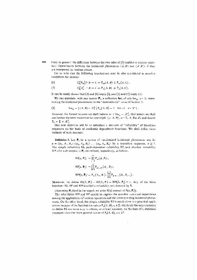
Let us note that the following implications may be also considered as possible candidates for axioms:

(6) T,[R„] I- B -> C => Pfl^(A, B) g PJA, C),

(7) T,[A] h B - C => PA(A, B) £ PA(A, C) .

It can be easily shown that (3) and (6) imply (i), and (3) and (7) imply (ii).

We can associate, with any system P„ a collection Inc, of sets Inc,,, (pel., repre­senting the incidental phenomena in the "deterministic" sense of Section 2:

(8) lnc9 = {<A, By e<??\PjA,B) = 1 for all a e E*} .

However, for formal reasons we shall behave as if Inc,, = ££\, that means we shall use further the term transition for any triple <<p, A, £>, q> e E, A, B e J^, and denote E, = X x &\.

Our next objective will be to introduce a measure of "reliability" of transition sequences on the basis of stochastic dependence functions. We shall define three variants of such measure.

Definition 3. Let P, be a system of randomized incidental phenomena and let a — Wi> Ax, 5i> ((p2,A2, B2y ... < >„, A„, B„y be a transition sequence, n S: 1. The simple reliability RS, path-dependent reliability RP, and Markov reliability RM of a with respect to P, are defined, respectively, as follows.

RS(a,P,) =flPjA,Bt), i = i

RP(a,P,) = f[ P„„jAlt Bt) , i = l

RM(a, P,) = PJAU Bt) 'UP9„,jAit B4+1) . i=i

Moreover, we define RS(A, P,) = RP(A, P,) = RM(A, P,) = 1. Any of the three functions RS, RP and RM is called a reliability and denoted by R.

(Assuming P, fixed in the sequel, we write R(a) instead of R(a, P,)). The reliabilities RM and RP enable to express the possible statistical dependence

among the applications of various operators and the corresponding incidental pheno­mena. On the other hand, the simple reliability RS is much close to a practical appli­cation because of the fact that the values PV(A, B), (pel, which are the only necessary to define RS are more easy to obtain, or at least estimate, on the base of a statistical treatment than the more general values of Pa(A, B), a e E*.

The reliability function and the stochastic dependence function are, according to Definition 3, closely interrelated. The former should be understood rather as a measure of "structural correctness" of transition sequences and depends on the incidental phenomena occurring in it; the latter expresses more the dynamical properties of the world with respect to a change indicated by an operator sequence.

The reliability, together with the function PA (the stochastic "distance" of formulas), are two measures which we shall use for evaluating approximate plans. As our first step towards introducing approximate plans we define an auxiliary structure, called 'quasi-plan', by abstraining from the requirement that the goal is achieved in a "uniform" way as in the case of deterministic plans of Definition 1, while retain­ing the inherent branching structure of the plan. (From now to the rest of the paper we keep fixed the underlying image space I, thus giving a permanent meaning to the symbols i f „ T„ Z, Z„ P„ R.)

Definition 4. Let X e Jz?, be a formula, let T ^ Zf be a nonempty (possibly infinite) set of transition sequences, and let F : Z* -» ££x be a function with the property that F(a) = false for all a e Zf — T. We shall call T a quasi-plan for X, and F a goal assigment for T, iff the following two conditions hold:

(0 r,[X]h V (Cop(r)&A t)v F(A); TEFA(r)

(ii) for each a == aY e Pref T ,

T,[Rop(t0 & Bz.~\ r V (Cop(t) & At) v F(a) . t£Fst(r)

Note that, if T is finite, by taking Y(fi) = Yfor each /? e T we obtain, as a particular case, the analyzed deterministic plan for {X, Y>.

Definition 5. Let <Z, Y> be a problem in I, let e, 8 ^ 0 be two real numbers. A finite nonempty set K c Z* is an (s, 8)-stochastic plan for (X, Y> and T ^ Zf is an analyzed (e, 5)-stochastic plan for (X, Y> [corresponding to K) iff K = op (T) and T is a quasi-plan for X with a goal assignment F such that for any a E T

(i) R(a) ^ 1 - s

(h) pA(n«). -0 £ - - * •

The intuitive idea behind the concept of an (e, c5)-stochastic plan can be explained as follows. We start with the analyzed deterministic plan for {X, Y> and generalize it by assuming that every branch terminates not necessarily reaching the goal Y but some another formula F(a) which is connected to Yonly stochastically: the condition (ii) expresses, in a stochastic way, the fact that F(a) is "close" to Y, or more precisely, that in a world satisfying F(a) there is a high probability (at least 1 - S) that Yholds, too. The condition (i) expresses the requirement that the reliability of any branch is at least 1 - £.

An example of a possible concrete goal assigment is F(A) = X if A e T and F(aT) = Rop(l) & Bz, if aT e T. The intuition for this choice may be that T is a frag­ment of a (larger) deterministic analyzed plan T'; (i.e. T S Pref T'); the only result known to have been achieved by a truncated branch ending by x is just Rop(t) & Bt. Hence, the considered goal assigment makes easier to test such fragments whether they are (e, (5)-stochastic plans or not.

The following two theorems establish the mutual relationship of (e, <5)-stochastic plans (with e = d = 0 and considering the simple reliability RS) and deterministic plans from Section 2. Let I be an image space with either Incl (a system of determi­nistic incidental phenomena) or P, (a system of randomized incidental phenomena). Let (X, Y) be a problem in I.

Theorem 1. Assume that, for every (pel,, <A, B) e Incv implies PV(A, B) = 1 and that R is the simple reliability RS. Then every (analyzed) deterministic plan for (X, Y) is also (analyzed) (0, 0)-stochastic plan for (X, Y).

Proof. Under the conditions of the theorem let K be a deterministic plan, and T a corresponding analyzed plan. Let a e T, then

R(a) = RS(a) = n P j A . , B ( ) >

where op (a) = q>i(p2 • • • <P„, < ;> B,) e Incp., i = 1, 2, . . . , n. Hence R(a) = 1. As any analyzed deterministic plan T is also a quasi-plan with respect to the uniform goal assigment F(a) = Y for all a e T , T, V Y-> Y hence, PA(Y Y) = 1 and thus K = op (T) is a (0, 0)-stochastic plan and T a corresponding analyzed (0,0)-stochastic plan.Q.E.D.

Theorem 2. Assume that for every <p e I

lnc,p = {(A,B)eJ?f\P<p(A,B)= 1} ,

moreover, assume that PA(A, B) = 1 implies T I- A ~> B for any A, B e Z£\ and that R is RS. Then every (analyzed) (0, 0)-stochastic plan for (X, Y) is also (analyzed) deterministic plan for (X, Y).

Proof. Under the conditions of the theorem let K be a (0, 0)-stochastic plan and T a corresponding analyzed (0, 0)-stochastic plan). Then T is a quasi-plan with a goal assignment F such that PA(F(a), Y) = 1 for any a e T . Thus T, h F(a) -* Y which enables to replace F(a) by Yin (ii) of Definition 4. We have

R(«)=RS(a) = I 1 P j A , 5 i . ) ,

where op (a) = (p u ...,cpn. By the condition R(a) = 1 we have PPi(A ;, B;) = 1,

i = 1, 2, . . . , n, hence <A;, 5,> e Inc,,.. The definition of a quasi-plan for this case

reduces to the definition of an analyzed deterministic plan, which yields the result

for r and thus also for K = op (E). Q.E.D.

Let us close this section by mentioning the fact that the model developed here

for representing the random character of problem domain is close to the model

introduced in [10]. The difference consists in the fact that in [10] the real-time

process of building a formal representation is emphasized and that this representa­

tion is of a special type.

4. UNBOUNDED PLANS: PLANS WITH LOOPS

Let us start our discussion of the second important modification of branching

plans with an illustrative example. It is a real-world situation requiring a plan with

iterations resembling WHILE loops in computer programs.

11 J2 I3 I4 lk jk.i JІЙ x

|R T T T т т п т т Fig. 1.

Example 1. Consider a long chain of rooms, numbered 1, 2, 3, . . . each pair

of adjacent rooms connected by a door (cf. Fig. l). There is a box in one of the rooms,

and a robot, initially in room 1, contemplates the problem of how to paint the box.

The robot's abilities consist of two operators

cp: go to the next room,

ij/: paint the box.

It is a fact of principal importance for our further reasoning that a solution of this

problem cannot be obtained on the basis of classical predicate logic by standard

methods of automatic plan formation, unless the total number of rooms is specified

at the beginning. In the latter case, i.e. if the total number of rooms is known to be

n (n 2: l), we can easily imagine a branching plan of the form

(9) {q>\jj | 0 g k < n}

obtained, let us say, on the basis of the situation calculus or the image space (cf. [17]).

The execution of plan (9) would follow a particular branch <pV iff the D 0 X is in the

(k + 1) st room (the robot has to enter k empty rooms before finding the box). Thus

the plan quarantees achieving the goal for any position of the box.

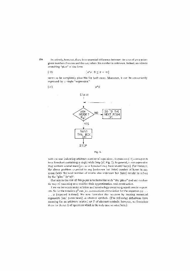
Intuitively, however, there is no essential difference between the case of an a priori given number of rooms and the case when this number is unknown. Indeed, an infinite branching "plan" of the form

(10) {ękф | 0 < k < 00}

seems to be completely plausible for both cases. Moreover, it can be conveniently

expressed by a single "expression"

(11) ę*ф

START

V N 0 > »•

/ в o x ^ \ v INSIDE?

V N 0 > »•

G0 T0 THE NEXT R00M

(Ф!

\ YES

•

V N 0 > »•

PAINT THE BOX

m

V N 0 > »•

STOP

Fig. 2.

with the star indicating arbitrary number of repetitions. Expression (11) corresponds to a flowchart containing a single while loop (cf. Fig. 2). In general, a star expression may contain several stars (just as a flowchart may have several loops). For instance, the above problem extended to any (unknown but finite) number of boxes in any room (with the total number of rooms also unknown but finite) would be solved by the "plan" (i/>>)*.

Our aim in the rest of this paper is to formalize such "star plans" and use stochas­tic way of reasoning as a tool for their approximation and construction.

First we introduce some notation and terminology concerning repetitions in sequen­ces. So far the notation cpk was just a convenient abbreviation for the sequence qxp . . . . . . <p (repeated fc-times). We now formalize this notation by treating numerical exponents (and parentheses) as abstract symbols. (The following definitions have meaning for an arbitrary original set S of abstract symbols; however, we formulate them for the set I of operators which is the only case we need here.)

Definition 6. The set Rp(E) of repetition expressions over E is the smallest set of formal expressions including E* and such that with each a, be Rp(E) and n e {1, 2, 3, . . . } also ab e Rp(E) and (a)" e Rp(E).

In this context we treat the numerals 1, 2, 3, . . . , n, ... as abstract symbols (codes) representing natural numbers. We interpret the repetition expressions in the natural way as sequences over E: for a = a e E* define \a\ = a and for a, be Rp(E), n 2: 1 define \ab\ = \a\ \b\ and |(a)"| = aa .. . a (w-times). Note that \a\ = \b\ does not, in general, imply a = b. For instance, |(<pi/03 <p| = \cp(tli<p)3\ = (p\ji(pii(p\l/(p. The numerals occuring in a repetition expression a are called the repetition indices in a.

We introduce star expressions as an extension of repetition expressions:

Definition 7. The set St (E) of star expressions over E is the smallest set of formal expressions including E* and such that with each a, b e St (E) and n 6 {1, 2, . . . } also al e St (E), (5)" e St (E) and (5)* e St (E).

Clearly E* £ Rp (E) E St (E). Unlike the repetition expressions the star expres­sions represent sets of sequences in accordance with the common interpretation of the Kleene star in formal language theory. Formally we define

J(a) = {a} , if 5 = a e E* ;

J(ab) ={ab\ae J(a), b e J(b)} ;

J((a)n) = {axa2 . . . a„ | a ; e J(a) for 1 ^ i ^ n} ;

J((a)*) = {A} u {axa2 ... a„ | 1 — n < oo and a ; e ,/(5) for 1 | i | nj .

Sequences in J(a) are called the repetition instances of a. We shall mostly work with a less general, but easier to manipulate, special class Ju(a) of uniform repetition instances: a e Ju(a) iff a = \a\ where a is a repetition expression obtained from 5 by formal replacement of all stars occuring in S by some repetition indices. We shall use a special notation for uniform repetition instances: assume 3 has n St 1 occurences of stars and let k = (klt . . . , fc„) e N" be the n-tuple (N is the set of positive integers) of the repetition indices in the repetition expression a, replacing all the stars of S (e.g. from the left to the right). Then we denote by a[k] or a\ku . . . , fc„] the corres­ponding uniform repetition instance of 5:

5[k] = |«] .

Thus, e.g.,

((<?)* W [2, 3] = (p<p\li(p<p\li<p(p\p

(note that nonuniform repetition instances, e.g. (pil/cpcpili, cannot be written in this way). In the following, whenever we write S[/c] we tacitly assume that k~ e N", where n S: 1 is the number of occurences of stars in 5.

We shall now introduce the main concept of this section.

Definition 8. Let <Z, Y> be a problem in the image space I. A finite nonempty set K £ St (2) is a stochastic star plan for {X, Y>, and a (possibly infinite) set T £ £f is an analyzed stochastic star plan for <Z, Y> (corresponding to K), iff

J(K) = op (r)

and r is a quasi-plan for X with a goal assigment F such that for every E > 0, 5 > 0 and every S e K there exists a e T such that op (a) is a uniform repetition of a and

(0 R ( a ) ^ l - E ,

(ii) PA(F(a), Y) ;> 1 - 8 .

In a strict analogy with our previous variants of the concept of a plan (Definition 1 and Definitions 4 and 5) we might be tempted to call a "plan" actually the set J(K)y

rather than K. We make this conceptual shift in order to preserve the common intuition of a plan as a finite structure which can serve as an input to a physical executing system. Here a plan K is just a finitary presentation of the possibly infinite set J"(K) which can be itself viewed as the set of all possible realizations of K. (As a matter of fact, already in the case of a deterministic plan we worked with the set of all possible realizations of a "real plan" represented, e.g., by a flow diagram.)

In the special case when K happens to be a subset of E* the concept of an (analyzed) stochastic star plan coincides with that of an (analyzed) (0, 0)-stochastic plan because of the finiteness of K (cf., also, Theorems 1 and 2).

The intuitive meaning of the last part of Definition 8 (beginning "for every e > 0, S > 0 . . . " ) can be explained als follows.

In a typical case one may expect that with increasing number of repetitions in op (a), and thus with increasing length of a, the possibility that the goal has been achieved increases. Thus for arbitralily small 8 the sequence a in (ii) may tend to be large. If, at the same time, the reliability is growing for large a, the condition (i) may be satisfied as well.

However, in reality every additional repetition is likely to increase the probability of a failure and consequently the function R(a) might, in fact, decrease. This is indeed the case when R is the simple reliability RS (cf. Definition 4); we shall return to this case below.

For this reason it may be interesting to give an example of a reliability function increasing with the number of repetitions. Consider two operators <p, i// and a star expression (<p)* i/> with an analyzing function/:

f((p"ilf) = <cp, Au B.> <<p, A2, B2} . . . <<p, An, B„} <&, A0, B0> .

Let

?9i(Au Bt) = 1

for Í = 1, 2, . . . , n and let

1 P„«ДAi, я 0 ) = i -

( + ì

When R is RP we have

R(j(<p») = [ n % ^ i . -».)] • ?*»Mi> BO) = i - — J - • i=i n + 1

This function is increasing and lim R(j(<p"i/')) = 1. (Intuition: think that cp is "strike

the nail by a hammer" and \j/ is "hang a picture on the nail").

Now consider the case of R = RS. The following theorem shows that under this

(and some other) general assumptions any set K, in order to be a plan in the sense

of Definition 8, has to possess a rather strong property, which, in fact, eliminates

the advantages of taking the reliability into account.

Let S e St (£) and let a, be J"a(a). We write a g b if either a = b or

a = a[k1, ..., fe„] and b = a[k[, ..., K] where kt ^ k[ for all i = 1, . . . , n. Let

us call an analyzing function j for 5 normal iff for each a, be •/„(«), if c ^ b, then

f(a) is a subsequence off(b) (i.e., all transitions inj(a) occur also inj(fo)).

Theorem 3. Let R = RS and let K be a stochastic star plan for a problem <X, Y> with an analyzing function j which is normal for all 5 e K. Then for every ae K and every 5 > 0 there exists a e ^U(S) such that

W*)) = i and

PA(Y(/(a)), Y)Zl-5,

Proof. Let ae K. If S is star-free then the result follows directly from Definition 8. Assume, therefore, that there is at least one occurence of the star in S. Denote by au a2, . . . e J^U(S) a sequence of uniform repetition instances of S such that R(/(af) ^ >. 1 — 1/i and PA(Y(/(a,)), Y) > 1 — 1/j; such a sequence exists according to the definition of stochastic star plan. R = RS gives that, for any a = (<<p;, A,-, B.>)"=i e e l f

R(a) = n P j A , , B , . ) . ; = i

The assumption o n / gives that if a. = a2, then any factor in the product for R(/(aj)) occurs also in the product for R(/(a2)), so R(f(a1)) ^ R(/(a2)). The number of star occurences in a is finite, hence, starting with certain element a„0 in the sequence above, any at is comparable with some ay, j < i. Hence, for any e0 > 0 there is only a finite number of values R(/(a,)) in (l — s0, 1>. Consequently there is an index

i0 such that / ^ i0 implies R(/(a:)) = 1. Taking; > /0 such that PA(F(/(a:)), Y) > d (that is always possible) and setting a = a} we obtain the conclusion of the theorem. Q.E.D.

This result reveals a rather restrictive nature of the notion of a stochastic plan, especially in combination with the simple reliability function. The whole idea of introducing randomnes into the plans is reduced just to the case when the "proximity" to the goal is evaluated. When the goal is approached only by a limiting process, the definition requires existence of arbitrarily long transition sequences of reliability one.

In the following variant of Definition 8 the reliability of sequences is kept only above certain predetermined value.

Definition 9. The z-stochastic star plan and the corresponding analyzed e-stochastic star plan are defined in the same way as stochastic star plans in Definition 8 except that the phrase "for every e > 0, 3 > 0 "is replaced by "for a fixed e S: 0 and every 5 > 0".

The following implications between the predicates 'stochastic' and 'e-stochastic' can be easily verified for star plans (and corresponding analyzed star plans) for a given problem:

(i) '0-stochastic' implies 'stochastic';

(ii) 'stochastic' implies 'e-stochastic' for any e > 0;

(iii) 'e-stochastic'implies'e'-stochastic'for any e' >. e.

Neither of these implications can be reversed, in general (note that the goal assignment involved in the definitions may depend on e). A particular case when 'stochastic' implies '0-stochastic' is represented in Theorem 3.

Let us illustrate the concepts of a stochastic and e-stochastic star plans using our example of a robot looking for a box.

Example 2. Let us simplify the situation from Example 1 by considering only one operator (p ("going to the next room") and a goal "finding the box". Our aim will be to examine in which extent the expression (9)* may represent an e-stochastic star plan for this problem.

First, we construct an image space I appropriate for this purpose. Let the core theory Tt include the axioms

3i ROBOT-IN(i)

(i.e., "the robot is in one of the rooms") and

3/ BOX-IN(j)

("the box is in one of the rooms"). The problem <X, Y> is expressed by the formulas 159

X = ROBOT-IN(l),

Y = 3i(ROBOT-IN(i) & BOX-IN(i)) .

An intuitive way of defining the operator cp would be to set

C„ = ROBOT-IN(fc), R„ = ROBOT-IN(fc + 1

("fc + 1" means "the (fc + l) st room") but this would make <p dependent on a para­meter fc which is not essential to the 'going-to-the-next-room', operator, and moreover, it would not yield a convenient randomization of the transfer from one room to another. For our purposes it is therefore advantageous to assume C^ = R„ = true and to treat pairs <ROBOT-IN(fc), ROBOT-IN(fc + l)> as incidental phenomena of (p. In addition, we can represent the fact that the position of the box does not change when the robot moves (a frame property) by incidental phenomena of the type <BOX-IN(fc), BOX-IN(fc)>; in our case we use their complementary form <~lBOX-IN(fc), "|BOX-IN(fc)>. To make easier our task let us describe (and later randomize) only those incidental phenomena which will be explicitly used in the analyzed stochastic plan corresponding to (q>)*. Define for fc ^ 1

k

Ak = ROBOT-IN(fc) & A nBOX-IN(i), !=1

k

Bk = ROBOT-IN(fc + 1)& A HBOX-IN(i) ; i = l

let xk = <qj, Ak, Bky and denote a0 = A and <xk = x^x2 e. . xk (fc S; 1). We suggest the set

r «-. {afc I k £ 0}

as a natural and appropriate solution to our problem. Indeed, it is just a formal way of expressing the following reasoning of the planning subject: "suppose that the fc-th room is entered (after fc — 1 repetitions of cp) and the box has not yet been found in any of the previous rooms (i.e., Bk-l holds). Now, the box is either in room fc and then the goal is achieved (Yholds) or the box is not in room fc (Ak holds) and then the only possibility is to go to the next, (fc + l) st room."

Let us consider the following stochastic dependence function

(12) P„.(Afc, -W.-x) = 1 - \ i

(i ^ 1) its values for other pairs of formulas will be irrelevant. Here r\ is an arbitrary constant, 0 < . » 7 < 1 . Ifjj + O, then (12) indicate an increase of the probability that repetitions of <p actually causes the change, say, from Ax to B,- (the possibility of a fail­ure to move to a next room is considered).

Let us now introduce the goal assigment Fas follows.

F(«0) = F(A) = X ;

Y(ak) = F ( T , ...rk)~Bk, fc ^ 1 .

In this way Y(ak) represents the planner's a priori knowledge of the world after the sequence ak has been realized. The probability that the goal has been achieved in such a world is measured by the function PA(Y(ak), Y). Let us choose

(13) PA(F(afc),Y) = l - / + 1 , (fc^O)

where p is a constant, 0 < p < 1 (such a function would be obtained, e.g., from an assumption that the box was placed in a room randomly according to Poisson di­stribution with parameter p).

We are now in the position to verify that the sets K = {(<p)*} and T• = {ak | k ^ 0} satisfy Definition 8, resp. 9. Clearly,

J(K) = {cpk\k^ 0} = op (T ) .

To show that T is a quasi-plan for X with the goal assigment F we observe that (i) and (ii) from Definition 4 obtain the respective forms

T,LY] r- A! v X and

T,[5,JhA4+1 v Bk,

both trivially valid. Let s > 0 and 8 > 0. Let us ask whether there is a number n = «£_a for which

the sequence a„ satisfies (i) and (ii) of Definition 8. We distinguish two cases for (i). First, if R = RS then by (12) (for i = 1)

R(a„) = nPp(A,,£,.) = ( l ->0"

and we obtain the inequality

(14) (1 - fj)» ^ 1 - s .

Second, if R = RP, then we obtain analogously the inequality

(15) n f l - ^ U l - a

Now to satisfy (ii) we obtain by (13) the unequality 1 - p" + 1 > 1 — 8, i.e.,

(16) 8 ^ p»+1 .

To satisfy (16) for arbitrarily small 8 we need arbitrarily large n.

In the case R = RS the conditions (i) and (ii) can be both satisfied only if fj = 0.

On the other hand, for R = RP, it is enough to take e ^ 1 - FJ (1 - f//i2) ^ 1 --nn2\6.

Thus we can conclude that (q>)* is an 2-star plan for <Z, Y> with respect to the path-dependent reliability RP iff s ^ nn2\6 and with respect to the simple reliability RS iff ^ = 0 and e ^ 0. (<?)* is a star plan for {X, Y> (with respect to RS or RP) iff ^ = 0. Note that, in agreement with Theorem 3, ^ = 0 implies RS(a„) = 1 for every n.

5. ASYMPTOTIC PROPERTIES OF STAR EXPRESSIONS

In the last section we have introduced the concept of a stochastic star plan based on the idea that considering all repetitions (of an operator or a sequence of operators) as one single entity (indicated by a star occurrence) enables goal-oriented planning even in cases when a lack of important knowledge of the world would make deter­ministic planning unfeasible. A closer look at the main definitions (Definitions 8 or 9) shows that the concept of a stochastic star plan has two aspects. The first concerns the branching structure of a plan (represented by the concept of a quasi-plan), the second is related to its approximating qualities — the reliability of transition sequences and the degree in which they approach the goal. In this section we shall be concerned with the second aspect.

First, we shall consider the question of reliability. Let a e St (S) be an arbitrary but fixed star expression. It may be desirable to associate directly with a its "reliability" say g(a)e(0, 1>. Two difficulties arise, however. First, star expressions consist of operators, while the reliability function R was defined for transition sequences. Therefore we shall always assume that an analyzing function / : J(a) -* Sf is available; recall that op f(a) = a for every a e J(a). Let us define

<?/(«) = KM) for each a e ^(a).

Second, star expressions represent possibly infinite sets of sequences. There are several intuitively plausible ways how to define Qf(a) on the basis of gf : <f(a) -» -> <0, 1>. For instance,

Qf(a) = ix\f{Qf(a)\aeJ(a)}

gf2\a) = sup {gf(a) | a e J(a)} .

The former reflects a pessimistic approach, the latter an optimistic one. There are, however, strong intuitive reasons for a definition of an asymptotic nature. Our

motivation for introducing stars was to use them as indicators of loops with un­bounded number of repetitions. In the execution time this number is, of course, finite (maybe small) but the planning system is unable to make any predictions of its value. One is therefore inclined to derive the reliability of a plan asymptotically from the reliability of its partial realizations with the number of repetitions growing unboundedly.

The following definition represents a number of possibilities according to the man­ner how the repetitions grow and whether we follow the best or the worst cases.

Definition 10. Let 3 e St (E) be a star expression, let n = 0 be the number of star occurrences in 5, let g : N" -> M and let j be an analyzing function for 3, The upper (resp. lower) asymptotic reliability of a (with respect to j and g), denoted by Qf,g(a) (resp. Qfi9(a)), is defined as follows. If n = 0 (i.e. if 3 = a e £*) then

QfM = QfM = Q/(\a\) • If ?! > 0 then

Qf,Xs) = l i m SUP QAS M ) 9(S)-oo

and QfJ?) = hminf !o /(3[/c]).

9(S)-oo

The function g determines the character of the limit, that is the topology with respect to which the limits are computed (any set {/c | g(k) > f} is a neighbourhood of the infinity).

Thus, for instance, to say that the upper (resp. lower) asymptotic reliability of 5 is greater than 1 — £ (e > 0) is the same as to say that for all (resp. for a sufficiently large) m > 0, infinitely many (resp. all) uniform repetition instances 3[/c] satisfying g(k~) > m have reliability greater than 1—8. Two natural examples of g are g = = min (yielding a topology equivalent to the ordinary Euclidean one) and g = max. In practice we would not, in general, compute the exact values of the asymptotic reliabilities. It is usually sufficient to know their lower estimates which may be often easy to obtain. For instance, to show that e/jinax(3) > 1 — e it is enough to choose an arbitrary infinite sequence of distinct repetition instances au a2, ..., from J"u(a) such that

lim R(f(a„)) > 1 - e .

Example 3. Continuing the case study from Example 2 we shall compute the asymptotic reliability of the expression (<p)* with respect to the analyzing function j(^>*) = ak a n d *° a n arbitrary increasing function, say, g(k) = k. For the case R = RS we have

QA<pk) = RS(afc) = (1 - t,f

and thus

QL((9)*) = QJJLW) = iim(i-.,y-{° iff *>0-

*->O0 [ 1 if )| = 0 .

For the case R = RP

, = i V Í 2

and thus

eL((<p)*) = <?;,(»*) - lim n ( i - \ ) 2; i - ^ n • k ^ o o i = i \ r / 6

We shall turn now to the question of degree in which a transition sequence ensures the goal. Once a plan is constructed it is not important which particular form of the goal assigment Y was used — what matters is just the proximity to the goal. We shall introduce a new concept of a <5-suitability of transition sequences.

Definition 11. Let a e Sf be a transition sequence, (X, y> a problem, and <5 = 0. We say that a is d-suitable for {X, Y) iff there is a formula Y' such that PA(Y', Y) = _ 1 - 5 and if a = A then

Tt[x] h r

else if the last transition in a is <<p, A, B> then

T,[R„ & B] h r .

Clearly, if a is <5-suitable for {X, Y) then it is ^'-suitable for any <5' = 3.

It appears that for representing the asymptotic properties of star expressions in a plan it is convenient to formalize a property that a given star expression admits repetition instances which have the corresponding transition sequences <5-suitable with <5 arbitrarily close to zero, and at the same time, of reliability arbitrarily close to one (the case of stochastic star plans), or above a certain predetermined level (the case of e-stochastic star plans). We arrive at the following definition.

Definition 12. Let 3 6 St ( I ) be a star expression with an analyzing function f, let (X, y> be a problem and let E > 0. We say that 3 is asymptotically suitable for <X, y> with the reliability level 1 — e iff for every <5 > 0 there exists a e ./u(a) such that

(i) f(a) is <5-suitable for <Z, y> and

(ii) of(a) = 1 - e.

Note that this definition admits a trivial "nonasymptotic" case, when some parti­cular repetition instance a e Jzr

u(«) is <5-suitable for arbitrary 8 > 0. If in addition

164 0f(a) jg 1 — e, then the defining property is fulfilled independently of other repeti­tion instances of a. When this does not happen we shall talk about asymptotic suitability in proper sense.

The following theorem relates the asymptotic suitability to e-stochastic star plans.

Theorem 4. Let (X, Y> be a problem, let £ > 0, let T £ Sf be a quasi-plan for X and let K S St (£) be such that ^(K.) = op (T) and each 3 e K is asymptotically suitable for (X, Y> with the reliability level 1 — e (and with respect to some analyzing function/ : ^u(3) -> T). Then K is an e-stochastic star plan (and T the corresponding analyzed e-stochastic star plan) for \X, Y>.

Proof. Under the assumptions of the theorem let Y be the goal-assignment that makes T a quasi-plan. By Definitions 11 and 12 (and denoting f(a) by a), for each ae K and each § > 0 there exists a = f(a) e T such that

op (a) = a 6 J"Ja),

R(a) = Qf(a) ^ 1 - e

and there exists Y'a such that PA(YX, Y) ^ 1 - <5 and

a = A implies T[Z] h F/, ,

a = a ' O , A, B} implies Ti[R,, & B] \- Ya.

Now to show that K and T satisfy the conclusion of the theorem it is enough to define for any a e Zf

„,r \ ( Y' if a satisfies the four conditions above, Y (a) = i

I Y(a) otherwise.

Clearly, T is a quasi plan with a goal assigment Y'. The theorem now follows directly from Definition 8 (rephrased according to Definition 9). Q.E.D.

It is interesting to note that Theorem 4 provides a stronger property than Defini­tion 8 (resp. 9). The difference is in the condition of ^-suitability of a which requires that, upon termination of a, Y' is provable, while in the definition of quasi-plan, there is assumed that Y(a) possibly in disjunction with other formulas (representing the continuing branches of the plan) is provable. Consequently, in the latter case the decision whether to determinate after executing op (a) has to be left for the execu­tion stage.

It is natural to investigate possibilities of practical testing of a given star expres­sion whether it is asymptotically suitable with respect to a given reliability level (or to determine such a level when it is not given).

A direct use of Definition 12 may appear rather difficult and we may look for cases where a specific knowledge of real properties of involved operators may be

helpful. A typical such case occurs when we are able to identify certain parts of a given expression whose repetitions influence essentially the suitability (through the para­meter S) and distinguish them from another parts influencing the reliability.

Consider, for instance, the expression ((<p)* \j/*) (think about our example of cp striking a nail and \ji hanging a picture; the above expression may be a plan for the task of "hanging all pictures"). Assume that the reliability of (<p"i/')m decreases with increasing m but increases with increasing n (as in the case discussed earlier) and that, on the other hand, the suitability increases with m (more pictures are hanged) and does not depend on n. In such a case it is quite natural first to study the suitability for m -* co ignoring the reliability (this corresponds to taking the reliability level 0, i.e. e = 1 in Definition 12), and then to work on n in order to obtain some higher reliability level.

In general, this idea of splitting the two components of asymptotic properties of star expressions may be often helpful. The computation may be even further simplified if we dispose of a value of some type of the asymptotic reliability from Definition 10.

Let us make our above considerations more specific. Consider a star expression 3 with an analyzing function j and assume that we already know that a is asympto­tically suitable for <Z, Y> with the reliability level zero. This means that we can construct an infinite sequence of (not necessarily distinct) tuples k\, k~2, ... such that for each 5 > 0 there exists i ^ 1 such that j(3[k;]) is (5-suitable for <X, Y>. Assume, moreover, that we know, independently, that

(17) Ql„(a) > 1 - e

for some function g. How combine these two facts? There may exist a procedure (hopefully an efficient one) associating with every fc; another tuple kj such that 5[k ;] is <5-suitab]e for the same 8 as 3[fc;] (without caring for the reliability) and the new sequence fc; has the property that for arbitrarily large m > 0 there exists i >_ 1 such that g(k'i) > m. If this happens we can conclude that 5 is asymptotically suitable for (X, 7> with the reliability level 1 - e.

Indeed, by Definition 10 and (17) there exists m0 > 0 such that for all k, g(k) > m0

implies j(5[fc]) > 1 — e. By the property of the sequence (fc;) there is then j > 1 such that

ef(s[kj]) > l - e

for all j S: i0. The conclusion then follows from the asymptotic suitability of (k;) and hence also of (fc;).

The situation may be simplified by an appropriate choice of the function g in (17) which determines the limiting character of asymptotic reliability. Considering, for instance, g = max (which enables using (k;) = (fc;)) we arrive at the following result which, as a particular case of our above reasoning does not require a separate proof.

Theorem 5. Let <X, y> be a problem and let a star expression 3 (with an analyzing function/) be asymptotically suitable for <X, Y} in proper sense, with the reliability level zero. Let

<?7,max(«) > 1 - S

for some e > 0. Then 5 is asymptotically suitable for {X, Y) with the reliability level 1 — e.

Let us apply this theorem to our running example.

Example 4. We claim that for the case of the robot looking for the box (cf. Example 2) the expression (q>)* (with the analyzing function f(<p") = a" and with R = RP) is asymptotically suitable for the problem (X, Y}, with the reliability level 1 — 2r\. For any <5 > 0 let n be large enough so that pn + 1 < 8. Then, by (13),

pA(y(a„), y) > I - 5,

i.e., due to the particular form of Y(a„), a„ = j(<p") is <5-suitable for {X, Y). At the same time, a„ is not <5'-suitable for 8' < p" + i (by assumption p > 0). Thus (<p)* is asymptotically suitable in proper sense for <X, y> with the reliability level 0. Now, since

07.m«((<P)*) = ] i m R p ( 0 = i - n — > i - 21 n-»o> 6

(cf. Example 3), our claim follows directly from Theorem 5.

6. GENERATING STAR PLANS

In the preceding sections we have developed an extensive formalism involving such concepts as (£, <5)-stochastic plan and e-stochastic star plan, which could serve as "approximate" solutions of problems when deterministic plans are difficult to obtain, or even when they do not exist. We have analyzed these concepts qualitatively from various aspects, including the reliability and suitability of a plan for a given problem. So far we have not, however, discussed the question how such approxim­ating plans can be effectively constructed. A theory, no matter how powerful, which would merely evaluate the performance of plans would be of little use if not accom­panied by an effective procedure for plan formation.

The main subject of this section is to outline a general method, called STAR-PLANNER, which converts a given set of transition sequences gradually into a set of star-expressions asymptotically suitable for a given problem (with a given relia­bility level). It is understood that the input set of STAR-PLANNER is obtained from a deterministic problem solver generating a (branching) plan or, in a general case,

a potentially infinite quasi-plan for the problem in question. This problem solver, called GENERATOR, combined with STAR-PLANNER, may thus serve as a promis-sing tool for generating e-stochastic star plans.

To elucidate this conception we shall first discuss deterministic plan formation. Let us start with a concrete, but rigorously tractable case of planning in situation calculus (cf. [17]). A problem <X, Y> obtains the form of an implicative formula

(18) X [ - 0 ] - 3s Y[s]

which expresses the statement "if X holds in the initial situation (s0) then there exists a goal situation (s) in which Y holds". This formula together with an axiomatic representation of the environment and of the robot's abilities, is put into an auto­matic theorem prover supplemented by an answer-extraction routine. If the formula (18) is provable the answer-extraction routine produces as its output a finite set of operator sequences which is a deterministic (branching) plan for <X, Y>.

It is obvious that the described way of generating plans is practically applicable only when the cardinality of the obtained set of sequences is rather small. In fact, the artificial intelligence literature often tacitly assumes plans consisting only of a single operator sequence (straight-line plans). The situation is quite different when the generated sets are untractably large or even infinite. This is exactly the point where our stochastic approach enters the scene.

It is important to view properly the both mentioned cases: the generated set is large but finite (a deterministic plan exists) or the generated set is infinite (there is no deterministic plan in the conventional sense). We argue that there are no practical reasons for distinguishing these two cases*). In the situation calculus the latter case occurs when the formula (18) is not provable: the theorem prover may in certain cases work without halting forever all the time producing new and new operator sequences (this possibility is inevitable due to the undecidability of the first-order predicate calculus). In spite of that the infinite set of successively generated transition sequences may have properties that qualify it intuitively as a genuine plan for the original problem (cf. Example l).

Our approach is based on two main theses. According to the first, even small finite fragments of large finite, or infinite, outputs of deterministic problem solvers are representative enough to be taken as a point of departure for approximate planning. According to the second thesis, even infinite set may be treated as an execut­able plan, provided it is presented in a finitistic way.

The first thesis concern GENERATOR. We shall abstract from its particular form, may it be a resolution theorem prover in situation calculus, an image space search method, or any other problem solver, provided it uses incidental phenomena. We assume that, with input <X, Y>, it generates successively transition sequences ai,a2, ...;

*) Making no distinction between large finite and infinite objects is characteristic for heuristic approaches in artificial intelligence.

each sequence a,- representing one branch in a would-be deterministic analyzed branching plan. What is essential is the requirement that GENERATOR produces analyzed operator sequences (elements of Zf) where the incidental phenomena actually used during the computation are explicitly indicated. (Note that the incidental phenomena are here understood in the deterministic sense as the system Incj; in STAR-PLANNER they will be replaced by the randomized system P,.) Formally, we could enforce our first thesis by the assumption that GENERATOR produces a quasi-plan, but we shall not need further such explicit requirement.

Our second thesis leads us to the conception of STAR-PLANNER as a procedure constructing a finite set of star expressions. The rough idea is that STAR-PLANNER alternately (i) asks GENERATOR for new sequences and (ii) makes guesses how to obtain asymptotically suitable star expressions such that some (preferably all) so far accumulated sequences are their repetition instances. Thus STAR-PLANNER may stop independently of the fact that GENERATOR does not have finished its work (this is the point where the distinction between the large finite and the infinite is dispensed with).

We shall present STAR-PLANNER in a semiformal way, purposely in the form of a highly nondeterministic algorithm. Every nondeterministic step is conceived as a possible point for implementing various heuristic hints. Some ideas for such heuristics as well as possible default decisions when no heuristics are available are mentioned at appropriate places.

The inputs to STAR-PLANNER, besides GENERATOR (which is called by STAR-PLANNER as its subroutine), are the problem (X, Y>, a reliability level 1 - e, a reliability function R (RS, RM or RP) and some other parameters which will be explained later. The procedure consists of eleven steps.

Step 1. Initialize F := 0; K := 0; i := 0.

[T £ Lf will hold for all the transition sequences produced by GENERATOR up to

a current step, K £ St (E) will be the set of star expressions under construction

(eventually the output) and i counts the sequences at produced by GENERATOR.]

Step 2. Set i := i + 1, a := ah T := T u {a}. If the GENERATOR refuses to give &i or if i exceeds a previously set limit go to Step 11.

Step 3. If R(a) ^ 1 - e0 and « is c50-suitable for <X, Y> go to Step 4. Otherwise go back to Step 2.

[Here E0, 30 e <0, 1> are parameters which select candidates for the starring pro­cedure in Steps 4 — 8. In practice Step 3 should be understood as only a partial test: unless the answer is easy to obtain it is considered to be negative.]

Step 4. Find a e Rp (£) such that op (a) = \a\.

[This is a nondeterministic step since there may be several repetition expressions for the same sequence (example: |(<p</')3 <p\ = |<p(i <p)3|). An informed heuristic would suggest the natural repetitions; in absence of such heuristics there is a simple default algorithm: search for shortest repeated subsequences from the left to the right, replace them by repetition expressions and iterate this procedure for thus obtained expression.]

Step 5. Let k be the number of occurences of repetition indices in a. Initialize*) •HIT : = &>{\,2, ...,k}.

Step 6. If W is empty go back to Step 2. Else select Qeif and construct the star expression b as follows: for each j e Q replace formally thej'-th occurence of a repe­tition index in a by a star occurence (in particular, if Q is empty, then b = a).

[The nondeterminism of this step is due to the phrase "select Q e W". This appears to be one of the most important places where a suitable heuristic should be chosen. An ideal heuristic would recognize those particular repetitions which indicate natural and/or necessary loops in the constructed plan and distinguish them from accidental repetitions. Due to the difficulty of finding such an ideal heuristic a practical imple­mentation may follow a more realistic "syntactically" controlled strategy. Such a strategy may be, for instance, based on the following suggestions:

(1) give the preference to Q with small cardinality (this yield star expressions with small number of stars);

(2) give the preference to inner, resp. outer, occurences of repetition indices (pre­ference to small, resp. large, loops);

(3) give the preference to large repetition indices (an important strategy based on the intuitively sound argument that a larger number of repetitions more likely indicates a loop);

(4) use the experience from the previous passes through Step 6 (this step is a part of a loop, cf. Step 8). In particular, there may be cases when the computation expen­ses for Steps 7 and 8 may be decreased, say, by selecting Q with the "previous Q" as a subset.]

Step 7. Specify an analyzing function/: Jjb) -> Sf such that / ( |a | ) = a.

[By "specify" we mean to give rules how to evaluate / when its value is needed (in Step 8). In general, Step 7 may appear rather difficult; however, in concrete cases the knowledge of a may be quite sufficient for extrapolating / to higher (or lower) repetitions.]

*) 0* denotes the power set, i.e. the set of all subsets.

Step 8. Test whether b is asymptotically suitable for {X, Y} with the reliability level 1 — £ (and with respect to analyzing function / ) . If not, either set W : = : = W — {Q] and return to Step 6 or (give up and) return to Step 2.

[The question of effective testing whether a given star expression is asymptotically suitable with a given reliability level was thoroughly analyzed in Section 4. The either-or-nondeterminism of Step 7 enables to leave the loop of Step 6 sooner than W is emptied, thus avoiding the maximum number of 2k passes. The heuristics for this nondeterminism may be combined with the heuristics for Step 6 and may be either static, e.g., by admitting the g's of only certain prespecified type, or dynamic, by learning from the previous passes.]

Step 9. Set K : = K u {£} and for all p e E check whether op (0) e J(K). If not re­turn to Step 2.

[Since K is a set of regular expressions the standard automata-theoretic techniques can be used for this purpose.]

Step 10. Halt. Output is K.

Step 11. Halt. Announce a failure.

It is clear that the set K produced by STAR-PLANNER consists entirely of star expressions asymptotically suitable for (X, Y> with the reliability level 1 — s (and with respect to appropriate analyzing function constructed in Step 7). However, in order that such K be an e-stochastic star plan, a necessary and sufficient condition would be, according to Theorem 4, that the corresponding set of analyzed sequences

rR = VM-fM

(different /= for different 3 e X, in general) is a quasi-plan for X.

Let us illustrate by an example how STAR-PLANNER works.

Example 5. Let us return to Example 1 with two operators

(p: "go to the next room" t/>: "paint the box"

and the task to paint the box. C^ and R,, were described in Example 2, let

Q = 3((ROBOT-IN(0&BOX-IN(i)),

R,A = BOX-PAINTED .

Consider a GENERATOR generating successively transition sequences a., a2> • • •

where a ; is

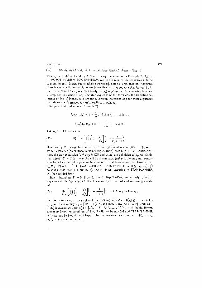
(19) <cp, Au Bj> <<p, A2, B 2 > . . . <<p, A„(i), B„ ( i )> <•>, 4» ( l ) + 1, B „ ( i ) + 1 >

with Aj, fe = n(i) + 1 and Bfc, k < n(i), being the same as in Example 2, -B„co+1

is "ROBOT-IN(n(/)) v BOX-PAINTED". We do not require the sequences a ; to be of monotonously increasing length (if i increases), suppose only, that any sequence of such a type will, eventually, occur (more formally, we suppose that for any/ e N there is i e N such that;' = n(ij). Clearly, op (a,) = <p"(j></< and the analyzing function is supposed to ascribe to any operator sequence of the form <pJij/ the transition se­quence as in (19) (hence, it is just the case when the values of / for other sequences than those already generated can be easily extrapolated).

Suppose that (unlike as in Example 2)

P Д A . , Bk) = 1 - ± ; 0 < ц < 1 , k š 1 ,

P Л (A>5* + . )= i -fe + 1

k > 0 .

Taking R = RP we obtain

(20) *w = [п(.-ÿ 40 +1 Denoting by C = C(n) the limit value of the right-hand side of (20) for n(i) —> co we can easily see (an exercise in elementary analysis), that C _ 1 — n. Considering, now, the star expression (tp)* \p (e St (S)) and using the definition of Qf, we obtain that 6f(((p)* "A) = c = 1 — V- As will be shown later, (q>)* \j/ is the only star expres­sion for which the value gf must be computed or at least minorized. Assume that PA(BJ+1, Y) = 1 - l/(i + 1) and recall that Y = BOX-PAINTED. Let 0 = e, e0, 80(< i ) be given such that 1] < min (e0, e). Other objects occuring in STAR-PLANNER will be specified later.

Step 1 initializes T : = 0, K : = 0, i : = 0. Step 2 offers, successively, operator sequences of the type cp'\j/, i _ 0 not necessarily in the order of increasing length. As

(21) um r n (Í - -Cíl I"1 - —^ = c = - - 1 > -.— LM V W J L í + d there is an index n0 = n0(n, e0) such that, for any n(i) < n0, R(a;) = 1 — E0 holds (if n = 0 then clearly n0 = [ l / £ - *])• A t t h e s a m e t i m e> PA(BI+U Y) tends to 1 if n(i) increases and, for n(i) > [l/<50 - 1], PA(l3„(i)+1, Y) = 1 - <50 holds. Hence, sooner or later, the condition of Step 3 will not be satisfied and STAR-PLANNER will continue by Step 4. Let it happen, for the first time, for a;; set n = n(i), a = a,-, £o> <>o < i g i v e s that n > 1.

Now, op (a) = cpn\\i. Considering, e.g., the heuristics trying to introduce as large

repetition indices as possible, we obtain the expression (cp)n \j> e Rp ( l ) with the pro­

perty that op (a) = (<p)n \j/, so Step 4 is executed. Trying to apply Step 5, we have

k = 2, iV = 3P{\, 2}. Selecting Q e W we may use a heuristic combining viewpoints

(l) and (3) mentioned after Step 5 when STAR-PLANNER described, i.e. we prefer to

replace by the star small number of high repetition indices, so we select {Q} = 1.

Executing Step 6 for a = op (a) we obtain, hence, b = (cp)* f. Step 7 establishes

an analyzing function / according to (19). As lim (l — l/(i + 1)) = 1, (21) holds

and both the limited functions are monotonously increasing, we can easily conclude

that (cp*) \p is asymptotically suitable with the level 1 — E, so the answer to Step 8

is positive and Step 9 follows. We set K = {b} and see that any ft e T is such that

op (p) = cp'ip for an i e N, so op (j8) e $(K) = J(b). Hence, STAR-PLANNER halts

after Step 10 giving K = {(cp)* \jj}.

(Received October 28, 1977.)

REFERENCES

[1] L. S. Coles et al.: Decision Analysis for an Experimental Robot with Unreliable Sensors. In: Proceedings of the 4th International Joint Conference on Artificial Intelligence, Tbilisi 1975, 749-757.

[2] R. O. Duda, P. E. Hart, N. J. Nilsson: Subjective Bayesian Methods for Rule-Based In­ference Systems. Research Report TN 124, Stanford Research Institute, 1976.

[3] J. A. Feldman, R. F. Sproull: Decision Theory and Artificial Intelligence II. Cognitive Science 1 (1977), No. 2.

[4] R. E. Fikes, P. E. Hart, N. J. Nilsson: Some New Directions in Robot Problem Solving. In: Machine Intelligence 7, Edinburgh University Press, 1972, 405 — 403.

[5] R. E. Fikes, P. E. Hart, N. J. Nilsson: Learning and Executing Generalized Robot Plans. Artificial Intelligence 3 (1972), 251-288.

[6] J. A. Goguen: On Fuzzy Robot Planning. In: Fuzzy Sets and their Applications to Cognitive and Decision Processes, New York, Academic Press, 1975.

[7] L. R. Harris: The Heuristic Search under Conditions of Error. Artificial Intelligence 5 (1974), 217-234.

[8] I. M. Havel, I. Kramosil: Probabilistic Methods in Robot Decision Making. In: Sbornik praci celostatni konference o kybernetice, Praha 1976, 66—80.

[9] W. Jacobs, M. Kiefer: Robot Decisions Based on Maximizing Utility. In: Proceedings of the 3rd International Joint Conference on Artificial Intelligence, Stanford 1973, 402—410.

[10] I. Kramosil: A Probabilistic Approach to Automaton-Environment Systems. Kybernetika 11 (1975), 3, 173-206.

[11] I. Kramosil: A probabilistic Restriction of Branching Plans, In: Mathematical Foundations of Computer Science, 1977, Lecture Notes in Computer Science 53, Springer Verlag, Ber l in-Heidelberg-New York 1977, 342-349.

[12] I. Kramosil: Probabilistic Restrictions of Branching Plans for Goal-Oriented Automaton Behaviour. (In Czech) Research Report, Institute of Information Theory and Automation, 1977.

[13] I. Kramosil: Some Remarks on Probabilities over Formalized Languages. Submitted for publication.

[14] J. H. Munson: Robot Planning, Execution and Monitoring in an Uncertain Environment. 173 In: Proceedings of the 2nd International Joint Conference on Artificial Intelligence, London 1971, 33S-349.

[15] J. Piper: Integrated Planning and Acting in a Stochastic Environment. Research Report, School of Artificial Intelligence, University of Edingburgh, 1972.

[16] L. Siklossy, J. Dreussi: Simulation of Executing Robots in Uncertain Environments, Rese­arch Report TR-16, Computer Science Department, University of Texas, 1973.

[17] O. Stepankova, I. M. Havel: A Logical Theory of Robot Problem Solving. Artificial In­telligence 7 (1976), 129-161.

[18] O. Stepankova, I. M. Havel: Incidental and State-Dependent Phenomena in Robot Problem Solving. Kybernetika 13 (1977), 6, 421—438 (cf. also the preliminary version In: Proceedings of the AISB Summer Conference, Edingburgh 1976, 266—278).

Ing. Ivan M. Havel, CSc Ph. D., Dr. Ivan Kramosil, CSc, Ustav teorie informace a aulomatizace CSA V (Institute of Information Theory and Automation — Czechoslovak Academy od Sciences), Pod voddrenskou vezi 4, 182 08 Praha 8. Czechoslovakia.