Distributed Multi-Robot Navigation in Formation among Obstacles:A Geometric and Optimization Approach with Consensus

Javier Alonso-Mora∗, Eduardo Montijano†, Mac Schwager‡ and Daniela Rus∗

Abstract— This paper presents a distributed method for navi-gating a team of robots in formation in 2D and 3D environmentswith static and dynamic obstacles. The robots are assumed tohave a reduced communication and visibility radius and shareinformation with their neighbors. Via distributed consensusthe robots compute (a) the convex hull of the robot positionsand (b) the largest convex region within free space. Therobots then compute, via sequential convex programming, thelocally optimal parameters for the formation within this convexneighborhood of the robots, allowing for reconfigurations,when required, by considering a set of target formations. Therobots navigate towards the target collision-free formation withindividual local planners that account for their dynamics. Theapproach is efficient and scalable with the number of robotsand performs well in simulations.

I. INTRODUCTION

Muti-robot teams can be employed for various tasks, suchas surveillance, inspection, or automated factories. In thesescenarios, robots may be required to navigate in formation,for example for maintaining a communication network, forcollaboratively handling an object, for surveilling an area orto improve navigation.

Multi-robot navigation in formation has received extensiveattention in the past, with many works considering obstacle-free scenarios. In [1] we leveraged efficient optimizationtechniques, namely quadratic programming, semi-definiteprogramming and (non-linear) sequential quadratic program-ming to devise a centralized method for local navigationin formation. These techniques provide good computationalefficiency, local guarantees and generality, and are employedat different stages of the method for local motion planningin formation among static and dynamic obstacles, albeitcentralized.

In this work we combine the optimization concepts pre-sented in [1] with distributed consensus and geometric rea-soning to achieve similar results in a distributed schema,where robots are no more centrally controlled, but insteadhave a limited field of view, and communicate with theirimmediate neighbors.

∗ The authors are at CSAIL-MIT, 32 Vassar St, 02139 Cambridge MA,USA {jalonsom,rus}@mit.edu† The author is with Centro Universitario de la Defensa, Zaragoza, Spain,

emonti@unizar.es‡ The author is with the Department of Aeronautics and

Astronautics, Stanford University, Stanford, CA 94305, USA,schwager@stanford.edu

*This work was supported in part by SMARTS N00014-09-1051, theBoeing Company, the MIT-Singapore Alliance on Research and Technologyunder the Future of Urban Mobility and by Spanish projects TELOMAN(DPI2012-32100), SIRENA (CUD2013-05) and grant CAS14/00205. Weare grateful for their support.

Given a set of target formation shapes, our method opti-mizes the parameters (such as position, orientation and size)of the multi-robot formation in a neighborhood of the robots.The method guarantees that the team of robots remainscollision-free by rearranging its formation. A simplifiedglobal planner, only waypoints for the formation center arerequired, can use this method to navigate the group of robotsfrom an initial location to a final location. But a humanmay also provide the global path for the formation, or adesired velocity, and the robots will adapt their configurationautomatically.

A. Related works

Extensive work exists for real-time navigation of multiplerobots in formation. These techniques include using a setof reactive behaviors [2], potential fields [3], navigationfunctions [4] and decentralized feedback laws with graph the-ory [5]. These have been mostly shown in 2D environmentsand may require extensive tuning for the particular formationand environment. In contrast, our method automatically opti-mizes for the formation parameters natively in a 2D and 3Ddynamic environment. On the down side, our method doesnot directly model the agent dynamics in the optimization,although it includes them in the individual local planners.

Distributed formation control solutions are also abundantin the literature [6]. The restriction of having a centralplanner can be easily lifted using nearest neighbors informa-tion [7]. These type of solutions usually rely on consensus-type controllers, e.g., [8], [9], or optimization methods [10],and assume the environment is obstacle-free. Compared tothem, we exploit consensus algorithms to obtain all thenecessary information to compute the optimal formation inthe presence of obstacles.

Convex optimization frameworks for navigating in forma-tion include semidefinite programming [11] which considersonly 2D circular obstacles, distributed quadratic optimiza-tion [12] without global coordination and limited adaptationof the formation, and second order cone programming [13]which triangulates the free 2D space to compute the optimalmotion in formation. In contrast, we propose a more generaloptimization plus consensus based approach.

Offline centralized non-convex optimizations include amixed integer approach [14] and a discretized linear temporallogic approach [15]. They provide global guarantees but scalepoorly with the number of robots. The second one is furtherlimited in the definition of the formation. In contrast, we aimat on-line computation, albeit local, by solving a non-linearprogram via sequential convex programming. This technique

target target

obstacle

target

(a) Independent target formations

target target

obstacle

target

(b) Independent obstacle-free regions

target target

obstacle

target

(c) Our approach

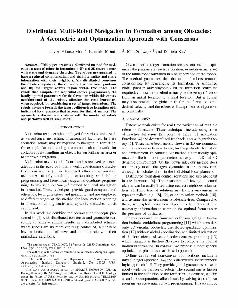
Fig. 1. Example of three approaches for distributed formation planning with obstacles as discussed in Sec. II. (a) Each robot independently computesa target formation (red/blue). Consensus on the formation’s parameters (green) would lead to a formation in collision with the obstacle. (b) Each robotcomputes an obstacle-free region, but their intersection is empty. (c) Our approach, see Sec. II, with target formation, after consensus, in green. Note that,in this example, the left most obstacle is not within the field of view of the robot in the right (blue region), but seen by the one in the left (red region).

has been employed [16] to compute collision-free trajectoriesfor multiple UAVs, but without considering formations.

B. Contribution

The main contribution of this paper is a distributed methodfor navigation of a team of robots while reconfiguring theirformation to avoid collisions. The method applies to robotsnavigating in 2D and 3D workspace among static and movingobstacles.

As part of our holistic method, we present distributedconsensus methods to compute (a) the convex hull of therobot’s positions and (b) the intersection of convex regions.We further rely on convex and non-convex optimizationtechniques first introduced in [1].

We provide a formal analysis with convergence guaranteesof the distributed algorithms composing the holistic approachand simulations with teams of robots.

C. Organization

Sec. II provides a high level overview of the whole ap-proach presented in the paper. Sec. III describes the notationand the centralized solution to the problem. Sec. IV describesthe main algorithm and Sec. V discusses experimental re-sults. Finally, the conclusions of the paper are in Sec. VI.

II. ALGORITHM OVERVIEW

Consider a team of robots, each with a limited field ofview, and a communication topology.

A naive approach could be that each robot computesa target formation and then all robots perform consensuson the formation parameters. Unfortunately, this can leadto a formation in collision with an obstacle, as shown inFigure 1(a). This problem can be solved if all the robotscompute a new formation in a common obstacle-free regionwhich is convex.

An approach to compute this common obstacle-free re-gion could be that each robot computes an obstacle-freeregion with respect to its limited field of view and thenthe robots collaboratively compute the intersection of allregions. Nonetheless, this could lead to an empty intersectionas shown in Figure 1(b).

This second problem can be solved by imposing that theconvex obstacle-free region computed by each robot accountsfor the robots’ positions, which is equivalent to it accountingfor the convex hull of the robots’ positions. See Figure 1(c)for an example.

Following this line of thought, the proposed method con-sists of the following steps.

1) Distributed computation of target formation:a) Robots perform distributed consensus to compute the

convex hull of the robots’ positions.b) Each robot computes the largest convex region in

obstacle-free space, grown from the convex hull of therobots’ positions and which is directed in the preferreddirection of motion.

c) Robots perform distributed consensus to compute theintersection of the individual convex regions.

d) Each robot computes the optimal target formationwithin the resulting convex volume.

e) Robots are assigned, with a distributed optimization, totarget positions within the target formation.

2) Collision-free motion towards the target formation:Robots, at a higher update rate, navigate towards theirassigned goals within the target formation. They locally avoidcollisions with their neighbors.

III. PRELIMINARIES

A. Definitions

1) Robots: Consider a team of robots navigating in for-mation. For each robot i ∈ I = {1, . . . , n} ⊂ N, its positionat time t is denoted by pi(t) ∈ R3. Let G = (I, E) bethe communication graph associated to the team of robots.Each edge in the graph, (i, j) ∈ E , denotes the possibilityof robots i and j to directly communicate with each other.The set of neighbors of robot i is denoted by Ni, i.e.,Ni = {j ∈ V | (i, j) ∈ E}. We assume that G is connected,i.e., for every pair of robots i, j there exists a path of oneor more edges in E that links robot i to robot j. We denoteby d the diameter of G, which is the longest among all theshortest paths between any pair of robots. In the followingwe consider all robots to have the same shape (cylinders).But the method is not strictly limited to this case.

2) Motion planning: This work presents an approach forlocal navigation. We consider that a desired goal positionfor the team of robots is given, and potentially known byall robots. This can be given by a human operator or astandard sampling based approach, and is outside the scopeof this work. Denote by g(t) ∈ R3 the goal position forthe centroid of the formation at time t. The distributed localplanner presented in this work computes a target formationand the required motion of the robots for a given time horizonτ > 0, which must be longer than the required time to stop.Denote the current time by to and tf = to + τ .

3) Static obstacles and field of view: For each robot i,its field of view, typically a sphere of given radius centeredat the robot’s position, is denoted by Bi ⊂ R3. Consider aset of static obstacles O ⊂ R3 defining the global map, andOi = Bi

⋂O the set of obstacles seen by robot i. Denote

by Oi the set Oi dilated by half of the robot’s volume, i.e.,the positions for which the robot of cylindrical shape wouldbe in collision with any of the obstacles within its visibilityradius.

4) Moving obstacles: Moving obstacles within the fieldof view of robot i can be accounted for. Consider j ∈ Ji ={1, . . . , nDO,i} ⊂ N the list of observed moving obstacles ofshape Dj ⊂ R3. We denote by Dj(t) the volume occupiedby the dynamic obstacle j at time t and Dj(t) its dilation byhalf of robot i’s volume. For predicted future positions weemploy the constant velocity assumption.

5) Position-time workspace: For robot i and current timeto denote the union of static and dynamic obstacles seen byrobot i by

Oi(to) = Oi × [0, τ ] ∪⋃

t∈[0,τ ]j∈Ji

Dj(to + t)× t ⊂ R4.

The position-time workspace for the robot is then

Wi(to) = R3 × [0, τ ] \ Oi(to) ⊂ R4. (1)

B. Formation definition

We consider a pre-defined set of f ∈ N default formations,such as square, line or T and known by all robots inthe team. Denote by F i0, 1 ≤ i ≤ f , one such defaultformation. Formation F i0 is given by a set of robot positions{ri0,1, . . . , ri0,n} and a set of vertices {fi0,1, . . . , f

i0,ni} relative

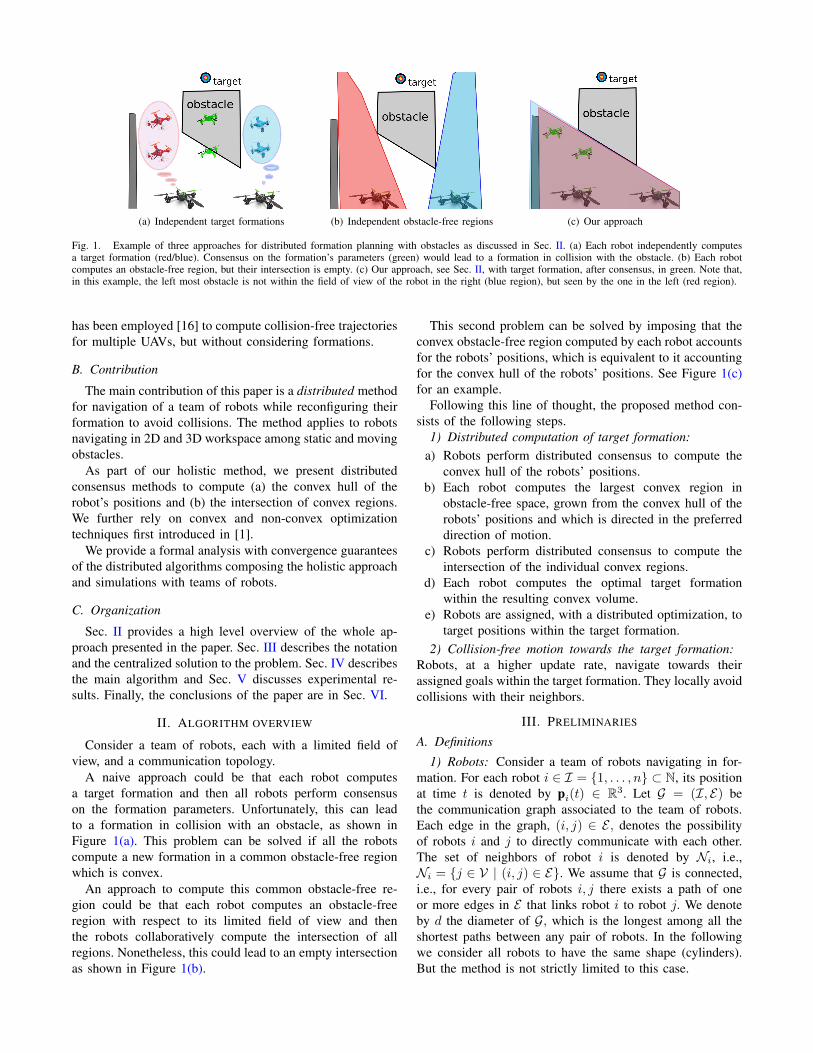
to the center of rotation (typically the centroid) of theformation. The set of vertices represents the convex hullof the robot’s positions in the formation, thus reducing thecomplexity for formations with a large number of robots.Denote by di0 the minimum distance between any given pairof robots in the default formation F i0. See Fig. 2 for anexample.

A formation is then defined by an isomorphic transforma-tion, which includes an expansion s ∈ R+, a translationt ∈ R3 and a rotation represented by a unit quaternionq ∈ SO(3), its conjugate denoted by q. The vector ofoptimization variables is denoted by x = [t, s,q] ∈ R8 andthe vertices and robot positions of the resulting formation

c

f1

f2

f3

f4

do

t

q

s

Fig. 2. Example of a square formation with sixteen disk robots andtransformed by x = [t, s, q]. The convex hull is given by vertices fj .

F i(x) are given by

rij = t + s rot(q, ri0,j), ∀j ∈ [1, n],

fij = t + s rot(q, fi0,j), ∀j ∈ [1, ni],(2)

where the rotation in SO(3) is given by[0 rot(q, x)

]T= q×

[0 x

]T × q. (3)

In the exposition of the method we rely on this definitionfor the formation, but the method is more general and can beapplied to alternative definitions, such as a team of mobilemanipulators carrying a rigid object. For that description ofthe formation, refer to Sec. V of the centralized method [1].

C. Centralized formation planningThe original algorithm for centralized local formation

planning [1] consists of the following steps.First, compute the largest convex polytope P in free space,

grown from the current robot positions, pi(to) ∈ P , ∀i ∈ I,and that is directed towards the goal g(tf ).

Second, compute the optimal formation F(tf ) containedwithin P and minimizing the distance between the for-mation’s centroid and the goal g(tf ). The parameters ofthe formation are optimized subject to a set of constraintsvia a centralized sequential convex optimization. In thiscomputation the robot’s dynamics are ignored.

Third, in a faster loop, the robots are optimally assignedto target positions of the formation F(tf ) and move towardsthem employing a low level local planner [17] that generatescollision-free inputs that respect the robot’s dynamics.

In the case that no feasible formation exists, the robotsnavigate independently towards the goal.

We extend this to distributed navigation in formation.

IV. DISTRIBUTED ALGORITHM

In this section we present the distributed algorithm tocompute the obstacle-free target formation. The algorithmaccounts for the limited visibility and communication ca-pabilities of all the robots by iterative message exchangeusing a consensus-type scheme. To avoid confusions in thenotation, throughout the section we denote discrete-timecommunication rounds using the index k and remove thecontinuous time dependency of the previous section. Weassume that the final time tf is longer than the amount oftime required for the distributed algorithm to compute theformation.

A. Convex hull of the robots’ positions

The first step the robots need to address to computethe target formation is the computation of the convex hull,C, of their positions. While this is a trivial problem incentralized scenarios, the same is not true in the currentcontext of limited communications because each robot onlyhas access to partial information. To overcome this limitationwe propose a distributed algorithm that allows all the robotsto obtain the convex hull of their positions using only localinteractions. In the algorithm we assume that there is afunction, convhull, that computes the convex hull spannedby a given set of points. Under this assumption, we let eachrobot handle a local estimation of the convex hull, Ci, thatis initialized containing exclusively the robot’s position, i.e.,Ci(0) = pi.

After that, the robots execute an iterative process whereat each iteration the local estimations are grown using theconvex hull estimations obtained by direct neighbors in thecommunication graph. Then, the robots communicate to theirneighbors only the new points that are part of their convexhull estimation, Ci(k) = Ci(k)\Ci(k−1). The whole processis repeated for a number of communication rounds equalto the diameter of G, d. This method is synthesized inAlgorithm 1.

Algorithm 1 Distributed Convex Hull - Robot i1: Ci(−1) = ∅, Ci(0) = pi2: for k = 0 . . . d− 1 do3: Send Ci(k) = Ci(k) \ Ci(k − 1) to all j ∈ Ni4: Receive Cj(k) from all j ∈ Ni5: Ci(k + 1) =convhull(Ci(k), Cj(k))6: end for

Proposition 1: The execution of Algorithm 1 makes thelocal estimation of all the robots converge to the actual con-vex hull of the whole team in no more than d communicationrounds. That is,

Ci(d) = C, ∀i ∈ I. (4)Proof: In order to show that (4) holds, we first show

by induction that

Ci(k + 1) = convhull(Ci(k), Cj(k)), (5)

for all i ∈ I, j ∈ Ni and k ≥ 0.Equation (5) holds for k = 1 because Ci(0) = Ci(0) =

pi and, therefore, for all i, Ci(1) =convhull(Ci(0), Cj(0)).Assume now that Eq. (5) is also true up to some other k > 0.Thus,

Ci(k + 1) = convhull(Ci(k), Cj(k))

= convhull(convhull(Ci(k − 1), Cj(k − 1)),

Cj(k) \ Cj(k − 1))

= convhull(Ci(k), Cj(k)),

where in the last equality we have accounted that all thepoints that are not sent by robot j are already contained inthe convex hull at the previous step of robot i.

Now let Ni(k), k ≥ 0, be the set of robots that arereachable from robot i after k propagation steps. That is,for k = 1, Ni(1) = Ni, whereas for k = 2, Ni(k) containsthe neighbors of robot i and the neighbors of its neighbors.In a second step we show that

Ci(k) = convhull(pi,pj), j ∈ Ni(k), (6)

for all k ≥ 0. Clearly Eq. (6) is true for k = 0 and k = 1.Assume that it is also true for some other k. Using (5),

Ci(k + 1) = convhull(Ci(k), Cj(k)),

= convhull(pi,pj), j ∈ Ni(k) ∪Nj(k)

= convhull(pi,pj), j ∈ Ni(k + 1).

By induction, since the communication graph is assumed tobe connected, Ni(d) = I and (4) holds.

In the worst case, where the convex hull contains thepositions of all the robots, our algorithm presents a com-munication cost equal to that of flooding all the positionsto all the robots. Nevertheless, even in such case, there arepractical advantages of using this procedure rather than pureflooding. Besides the likely savings in communications frompositions that are not relayed because they do not belongto the convex hull, with our procedure there is no need fora specific identification of which position corresponds to aparticular robot, making it better suited for pure broadcastimplementations.

Remark 1 (Unknown d or changing networks): If the di-ameter, d, is unknown, the consensus runs until convergencefor all robots. Since only new points are transmitted at eachiteration, the convergence of the algorithm can be detectedusing a timeout when no new messages are received. Usingthis strategy our algorithm can also be used in the presence ofchanges in the communication graph, as long as the typicalassumption of periodic joint connectivity occurs [7].

B. Obstacle-free convex region

Denote by g ∈ R3 the goal position for the robot formationand consider it known by all robots. Recall that, from theprevious step, all robots have knowledge of the convex hullC of the robots’ positions. With this common information,but different obstacle map due to the limited field of view,each robot computes a obstacle-free convex region embeddedin position - time space, denoted Pi ∈ R3 × [0, τ ].

Analogously to the derivations in [1], Pi is given by theintersection of two convex polytopes, both directed towardsthe goal g, the first one containing C and the second onecontaining only the centroid of C, denoted by c ∈ R3.Following the notation therein, the convex polytope is thengiven by Pi = Pfo→g|i ∩ Po→g|i = P [g,τ ]

C×0 (Wi(to)) ∩P [g,τ ]

c×0 (Wi(to)) ⊂ Wi(to).Pi guarantees that the transition to the new formation, and

the transition, will be obstacle-free (from [C × 0] ⊂ Pfo→g|iand Pi ⊂ Pfo→g|i) and is likely to make progress in futureiterations (Pi ⊂ Po→g). The convex regions are grownin the direction towards the goal g following an iterativeoptimization [18] as described in [1].

However, due to the local visibility of the robots, some ofthese regions may intersect some obstacles that a particularrobot has not seen. Additionally, these regions might not beequal for all robot, which, if used without further agreement,would lead to different target formations. Thus, the robotsneed to agree upon a common region that is globally freeof obstacles. For that purpose, we next propose a distributedalgorithm that computes the intersection of all the regions,P =

⋂i∈I Pi.

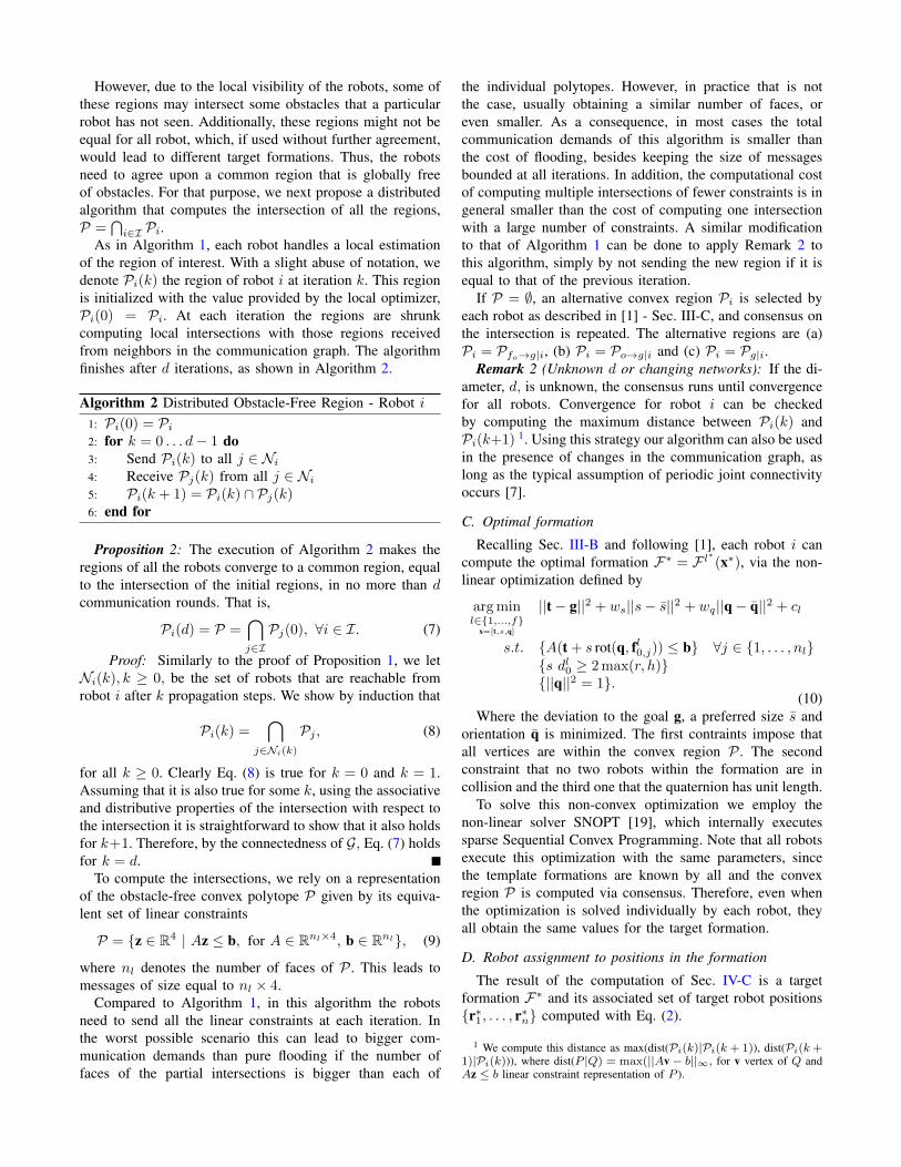
As in Algorithm 1, each robot handles a local estimationof the region of interest. With a slight abuse of notation, wedenote Pi(k) the region of robot i at iteration k. This regionis initialized with the value provided by the local optimizer,Pi(0) = Pi. At each iteration the regions are shrunkcomputing local intersections with those regions receivedfrom neighbors in the communication graph. The algorithmfinishes after d iterations, as shown in Algorithm 2.

Algorithm 2 Distributed Obstacle-Free Region - Robot i1: Pi(0) = Pi2: for k = 0 . . . d− 1 do3: Send Pi(k) to all j ∈ Ni4: Receive Pj(k) from all j ∈ Ni5: Pi(k + 1) = Pi(k) ∩ Pj(k)6: end for

Proposition 2: The execution of Algorithm 2 makes theregions of all the robots converge to a common region, equalto the intersection of the initial regions, in no more than dcommunication rounds. That is,

Pi(d) = P =⋂j∈IPj(0), ∀i ∈ I. (7)

Proof: Similarly to the proof of Proposition 1, we letNi(k), k ≥ 0, be the set of robots that are reachable fromrobot i after k propagation steps. We show by induction that

Pi(k) =⋂

j∈Ni(k)

Pj , (8)

for all k ≥ 0. Clearly Eq. (8) is true for k = 0 and k = 1.Assuming that it is also true for some k, using the associativeand distributive properties of the intersection with respect tothe intersection it is straightforward to show that it also holdsfor k+1. Therefore, by the connectedness of G, Eq. (7) holdsfor k = d.

To compute the intersections, we rely on a representationof the obstacle-free convex polytope P given by its equiva-lent set of linear constraints

P = {z ∈ R4 | Az ≤ b, for A ∈ Rnl×4, b ∈ Rnl}, (9)

where nl denotes the number of faces of P . This leads tomessages of size equal to nl × 4.

Compared to Algorithm 1, in this algorithm the robotsneed to send all the linear constraints at each iteration. Inthe worst possible scenario this can lead to bigger com-munication demands than pure flooding if the number offaces of the partial intersections is bigger than each of

the individual polytopes. However, in practice that is notthe case, usually obtaining a similar number of faces, oreven smaller. As a consequence, in most cases the totalcommunication demands of this algorithm is smaller thanthe cost of flooding, besides keeping the size of messagesbounded at all iterations. In addition, the computational costof computing multiple intersections of fewer constraints is ingeneral smaller than the cost of computing one intersectionwith a large number of constraints. A similar modificationto that of Algorithm 1 can be done to apply Remark 2 tothis algorithm, simply by not sending the new region if it isequal to that of the previous iteration.

If P = ∅, an alternative convex region Pi is selected byeach robot as described in [1] - Sec. III-C, and consensus onthe intersection is repeated. The alternative regions are (a)Pi = Pfo→g|i, (b) Pi = Po→g|i and (c) Pi = Pg|i.

Remark 2 (Unknown d or changing networks): If the di-ameter, d, is unknown, the consensus runs until convergencefor all robots. Convergence for robot i can be checkedby computing the maximum distance between Pi(k) andPi(k+1) 1. Using this strategy our algorithm can also be usedin the presence of changes in the communication graph, aslong as the typical assumption of periodic joint connectivityoccurs [7].

C. Optimal formation

Recalling Sec. III-B and following [1], each robot i cancompute the optimal formation F∗ = F l∗(x∗), via the non-linear optimization defined by

arg minl∈{1,...,f}

x=[t,s,q]

||t− g||2 + ws||s− s||2 + wq||q− q||2 + cl

s.t. {A(t + s rot(q, fl0,j)) ≤ b} ∀j ∈ {1, . . . , nl}{s dl0 ≥ 2 max(r, h)}{||q||2 = 1}.

(10)Where the deviation to the goal g, a preferred size s and

orientation q is minimized. The first contraints impose thatall vertices are within the convex region P . The secondconstraint that no two robots within the formation are incollision and the third one that the quaternion has unit length.

To solve this non-convex optimization we employ thenon-linear solver SNOPT [19], which internally executessparse Sequential Convex Programming. Note that all robotsexecute this optimization with the same parameters, sincethe template formations are known by all and the convexregion P is computed via consensus. Therefore, even whenthe optimization is solved individually by each robot, theyall obtain the same values for the target formation.

D. Robot assignment to positions in the formation

The result of the computation of Sec. IV-C is a targetformation F∗ and its associated set of target robot positions{r∗1, . . . , r∗n} computed with Eq. (2).

1 We compute this distance as max(dist(Pi(k)|Pi(k + 1)), dist(Pi(k +1)|Pi(k))), where dist(P |Q) = max(||Av− b||∞, for v vertex of Q andAz ≤ b linear constraint representation of P ).

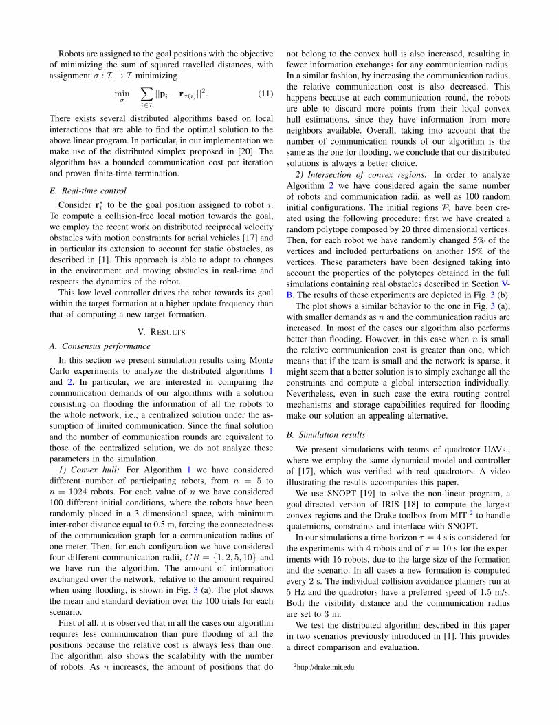
Robots are assigned to the goal positions with the objectiveof minimizing the sum of squared travelled distances, withassignment σ : I → I minimizing

minσ

∑i∈I||pi − rσ(i)||2. (11)

There exists several distributed algorithms based on localinteractions that are able to find the optimal solution to theabove linear program. In particular, in our implementation wemake use of the distributed simplex proposed in [20]. Thealgorithm has a bounded communication cost per iterationand proven finite-time termination.

E. Real-time control

Consider r∗i to be the goal position assigned to robot i.To compute a collision-free local motion towards the goal,we employ the recent work on distributed reciprocal velocityobstacles with motion constraints for aerial vehicles [17] andin particular its extension to account for static obstacles, asdescribed in [1]. This approach is able to adapt to changesin the environment and moving obstacles in real-time andrespects the dynamics of the robot.

This low level controller drives the robot towards its goalwithin the target formation at a higher update frequency thanthat of computing a new target formation.

V. RESULTS

A. Consensus performance

In this section we present simulation results using MonteCarlo experiments to analyze the distributed algorithms 1and 2. In particular, we are interested in comparing thecommunication demands of our algorithms with a solutionconsisting on flooding the information of all the robots tothe whole network, i.e., a centralized solution under the as-sumption of limited communication. Since the final solutionand the number of communication rounds are equivalent tothose of the centralized solution, we do not analyze theseparameters in the simulation.

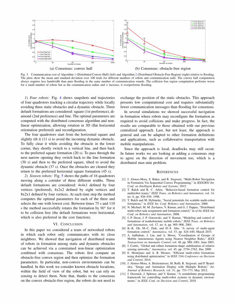
1) Convex hull: For Algorithm 1 we have considereddifferent number of participating robots, from n = 5 ton = 1024 robots. For each value of n we have considered100 different initial conditions, where the robots have beenrandomly placed in a 3 dimensional space, with minimuminter-robot distance equal to 0.5 m, forcing the connectednessof the communication graph for a communication radius ofone meter. Then, for each configuration we have consideredfour different communication radii, CR = {1, 2, 5, 10} andwe have run the algorithm. The amount of informationexchanged over the network, relative to the amount requiredwhen using flooding, is shown in Fig. 3 (a). The plot showsthe mean and standard deviation over the 100 trials for eachscenario.

First of all, it is observed that in all the cases our algorithmrequires less communication than pure flooding of all thepositions because the relative cost is always less than one.The algorithm also shows the scalability with the numberof robots. As n increases, the amount of positions that do

not belong to the convex hull is also increased, resulting infewer information exchanges for any communication radius.In a similar fashion, by increasing the communication radius,the relative communication cost is also decreased. Thishappens because at each communication round, the robotsare able to discard more points from their local convexhull estimations, since they have information from moreneighbors available. Overall, taking into account that thenumber of communication rounds of our algorithm is thesame as the one for flooding, we conclude that our distributedsolutions is always a better choice.

2) Intersection of convex regions: In order to analyzeAlgorithm 2 we have considered again the same numberof robots and communication radii, as well as 100 randominitial configurations. The initial regions Pi have been cre-ated using the following procedure: first we have created arandom polytope composed by 20 three dimensional vertices.Then, for each robot we have randomly changed 5% of thevertices and included perturbations on another 15% of thevertices. These parameters have been designed taking intoaccount the properties of the polytopes obtained in the fullsimulations containing real obstacles described in Section V-B. The results of these experiments are depicted in Fig. 3 (b).

The plot shows a similar behavior to the one in Fig. 3 (a),with smaller demands as n and the communication radius areincreased. In most of the cases our algorithm also performsbetter than flooding. However, in this case when n is smallthe relative communication cost is greater than one, whichmeans that if the team is small and the network is sparse, itmight seem that a better solution is to simply exchange all theconstraints and compute a global intersection individually.Nevertheless, even in such case the extra routing controlmechanisms and storage capabilities required for floodingmake our solution an appealing alternative.

B. Simulation results

We present simulations with teams of quadrotor UAVs.,where we employ the same dynamical model and controllerof [17], which was verified with real quadrotors. A videoillustrating the results accompanies this paper.

We use SNOPT [19] to solve the non-linear program, agoal-directed version of IRIS [18] to compute the largestconvex regions and the Drake toolbox from MIT 2 to handlequaternions, constraints and interface with SNOPT.

In our simulations a time horizon τ = 4 s is considered forthe experiments with 4 robots and of τ = 10 s for the exper-iments with 16 robots, due to the large size of the formationand the scenario. In all cases a new formation is computedevery 2 s. The individual collision avoidance planners run at5 Hz and the quadrotors have a preferred speed of 1.5 m/s.Both the visibility distance and the communication radiusare set to 3 m.

We test the distributed algorithm described in this paperin two scenarios previously introduced in [1]. This providesa direct comparison and evaluation.

2http://drake.mit.edu

5 16 64 256 10240

0.2

0.4

0.6

0.8

1

1.2

1.4

1.6

1.8

Number of robots

% o

f dat

a se

ntco

mpa

red

to fl

oodi

ng

Com Rad 1mCom Rad 2mCom Rad 5mCom Rad 10m

5 16 64 256 10240

0.2

0.4

0.6

0.8

1

1.2

1.4

1.6

1.8

Number of robots

% o

f dat

a se

ntco

mpa

red

to fl

oodi

ng

Com Rad 1mCom Rad 2mCom Rad 5mCom Rad 10m

(a) Consensus: convex hull (b) Consensus: obstacle-free regionFig. 3. Communication cost of Algorithm 1 (Distributed Convex Hull) (left) and Algorithm 2 (Distributed Obstacle-Free Region) (right) relative to flooding.The plots show the mean and standard deviation over 100 trials for different numbers of robots and communication radii. The convex hull computationalways requires less bandwidth than pure flooding in the same number of communication rounds. The collision free region computation performs worsefor a small number of robots but as the communication radius and n increase, it overperforms flooding.

1) Four robots: Fig. 4 shows snapshots and trajectoriesof four quadrotors tracking a circular trajectory while locallyavoiding three static obstacles and a dynamic obstacle. Threedefault formations are considered: square (1st preference), di-amond (2nd preference) and line. The optimal parameters arecomputed with the distributed consensus algorithm and non-linear optimizaiton, allowing rotation in 3D (flat horizontalorientation preferred) and reconfiguration.

The four quadrotors start from the horizontal square andslightly tilt it (11 s) to avoid the incoming dynamic obstacle.To fully clear it while avoiding the obstacle in the lowercorner, they shortly switch to a vertical line, and then backto the preferred square formation (20 s). To pass through thenext narrow opening they switch back to the line formation(30 s) and then to the preferred square, tilted to avoid thedynamic obstacle (37 s). Once the obstacles are cleared theyreturn to the preferred horizontal square formation (45 s).

2) Sixteen robots: Fig. 5 shows the paths of 16 quadrotorsmoving along a corridor of three different widths. Threedefault formations are considered: 4x4x1 defined by fourvertices (preferred), 4x2x2 defined by eight vertices and8x2x1 defined by four vertices. At each time step the methodcomputes the optimal parameters for each of the three andselects the one with lowest cost. Between times 75 s and 110s the method successfully rotates the formation by 90o for itto be collision free (the default formations were horizontal,which is also preferred in the cost function).

VI. CONCLUSION

In this paper we considered a team of networked robotsin which each robot only communicates with its closeneighbors. We showed that navigation of distributed teamsof robots in formation among static and dynamic obstaclescan be achieved via a constrained non-linear optimizationcombined with consensus. The robots first compute anobstacle-free convex region and then optimize the formationparameters. In particular, non-convex environments can behandled. In this work we consider known obstacle locations,within the field of view of the robot, but we can rely onsensing to detect them. Note that, thanks to the consensuson the convex obstacle-free region, the robots do not need to

exchange the position of the static obstacles. This approachpresents low computational cost and requires substantiallyfewer communication messages than flooding for consensus.

In several simulations we showed successful navigationin formation where robots may reconfigure the formation asrequired to avoid collisions and make progress. In fact, theresults are comparable to those obtained with our previouscentralized approach. Last, but not least, the approach isgeneral and can be adapted to other formation definitionsand applications, such as collaborative transportation withmobile manipulations.

Since the approach is local, deadlocks may still occur.In future works we are looking at adding a consensus stepto agree on the direction of movement too, which is adistributed max-min problem.

REFERENCES

[1] J. Alonso-Mora, S. Baker, and R. Siegwart, “Multi-Robot Navigationin Formation Via Sequential Convex Programming,” in IEEE/RSJ Int.Conf. on Intelligent Robots and Systems, 2015.

[2] T. Balch and R. C. Arkin, “Behavior-based formation control formultirobot teams,” IEEE Trans. on Robotics and Automation, vol. 14,no. 6, pp. 926–939, 1998.

[3] T. Balch and M. Hybinette, “Social potentials for scalable multi-robotformations,” in IEEE Int. Conf. Robotics and Automation, 2000.

[4] N. Michael, M. M. Zavlanos, V. Kumar, and G. J. Pappas, “Distributedmulti-robot task assignment and formation control,” in of the IEEE Int.Conf. on Robotics and Automation, 2008.

[5] J. P. Desai, J. P. Ostrowski, and V. Kumar, “Modeling and control offormations of nonholonomic mobile robots,” IEEE Trans. on Roboticsand Automation, vol. 17, no. 6, pp. 905–908, 2001.

[6] K.-K. Oh, M.-C. Park, and H.-S. Ahn, “A survey of multi-agentformation control,” Automatica, vol. 53, pp. 424–440, March 2015.

[7] A. Jadbabaie, J. Lin, and A. Morse, “Coordination of Groups ofMobile Autonomous Agents using Nearest Neighbor Rules,” IEEETransactions on Automatic Control, vol. 48, pp. 988–1001, June 2003.

[8] J. Cortes, “Global and robust formation-shape stabilization of relativesensing networks,” Automatica, vol. 45, pp. 2754–2762, Dec 2009.

[9] E. Montijano and A. R. Mosteo, “Efficient multi-robot formationsusing distributed optimization,” in IEEE 53th Conference on Decisionand Control, 2014.

[10] J. Alonso-Mora, A. Breitenmoser, M. Rufli, R. Siegwart, and P. Beard-sley, “Image and Animation Display with Multiple Robots,” Int.Journal of Robotics Research, vol. 31, pp. 753–773, May 2012.

[11] J. Derenick, J. Spletzer, and V. Kumar, “A semidefinite programmingframework for controlling multi-robot systems in dynamic environ-ments,” in IEEE Conf. on Decision and Control, 2010.

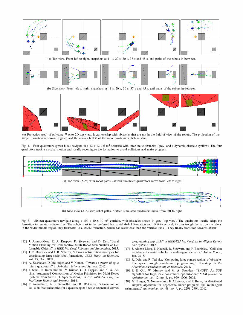
(a) Top view. From left to right, snapshots at 11 s, 20 s, 30 s, 37 s and 45 s, and paths of the robots in-between.

(b) Side view. From left to right, snapshots at 11 s, 20 s, 30 s, 37 s and 45 s, and paths of the robots in-between.

(c) Projection (red) of polytope P onto 2D top view. It can overlap with obstacles that are not in the field of view of the robots. The projection of thetarget formation is shown in green and the convex hull C of the robot positions with blue stars.

Fig. 4. Four quadrotors (green-blue) navigate in a 12 x 12 x 6 m3 scenario with three static obstacles (grey) and a dynamic obstacle (yellow). The fourquadrotors track a circular motion and locally reconfigure the formation to avoid collisions and make progress.

(a) Top view (X-Y) with robot paths. Sixteen simulated quadrotors move from left to right.

(b) Side view (X-Z) with robot paths. Sixteen simulated quadrotors move from left to right.

Fig. 5. Sixteen quadrotors navigate along a 100 x 10 x 10 m3 corridor, with obstacles shown in grey (top view). The quadrotors locally adapt theformation to remain collision free. The robots start in the preferred horizontal 4x4x1 formation and tilt it to vertical, to pass trough the narrow corridors.In the wider middle region they transform to a 4x2x2 formation, which has lower cost than the vertical 4x4x1. They finally transition towards 4x4x1.

[12] J. Alonso-Mora, R. A. Knepper, R. Siegwart, and D. Rus, “LocalMotion Planning for Collaborative Multi-Robot Manipulation of De-formable Objects,” in IEEE Int. Conf. Robotics and Automation, 2015.

[13] J. C. Derenick and J. R. Spletzer, “Convex optimization strategies forcoordinating large-scale robot formations,” IEEE Trans. on Robotics,vol. 23, Dec. 2007.

[14] A. Kushleyev, D. Mellinger, and V. Kumar, “Towards a swarm of agilemicro quadrotors,” in Robotics: Science and Systems, 2012.

[15] I. Saha, R. Ramaithitima, V. Kumar, G. J. Pappas, and S. A. Se-shia, “Automated Composition of Motion Primitives for Multi-RobotSystems from Safe LTL Specifications,” in IEEE/RSJ Int. Conf. onIntelligent Robots and Systems, 2014.

[16] F. Augugliaro, A. P. Schoellig, and R. D’Andrea, “Generation ofcollision-free trajectories for a quadrocopter fleet: A sequential convex

programming approach,” in IEEE/RSJ Int. Conf. on Intelligent Robotsand Systems, 2012.

[17] J. Alonso-Mora, T. Naegeli, R. Siegwart, and P. Beardsley, “Collisionavoidance for aerial vehicles in multi-agent scenarios,” Auton. Robot.,Jan. 2015.

[18] R. Deits and R. Tedrake, “Computing large convex regions of obstacle-free space through semidefinite programming,” Workshop on theAlgorithmic Fundamentals of Robotics, 2014.

[19] P. E. Gill, W. Murray, and M. A. Saunders, “SNOPT: An SQPalgorithm for large-scale constrained optimization,” SIAM journal onoptimization, vol. 12, no. 4, pp. 979–1006, 2002.

[20] M. Burger, G. Notarstefano, F. Allgower, and F. Bullo, “A distributedsimplex algorithm for degenerate linear programs and multi-agent

assignments,” Automatica, vol. 48, no. 9, pp. 2298–2304, 2012.