a structural design guide for flexible residential …
TRANSCRIPT

S
6~5.7(94) I $a AUS
41 I TO A NEW AGE OF PAVEMENT DESIGN
A STRUCTURAL DESIGN GUIDE FOR FLEXIBLE RESIDENTIAL STREET PAVEMENTS
Superseded
By P. J. Mulholland Senior Research Scienllst
Special Report No. 41 ~~ AUSTRALIAN ROAD RESEARCH BOARD ~ "liliiii

Since Special Report 41 was published in 1989, there have been a
number of subsequent publications offering more current guidance.
Present advice is to review the Austroads Guide to pavement
technology: Part 2: Pavement structural design, published in 2012
(AGPT 02/12).
, I 'l ~
" ,
!
INTO A NEW AGE OF PAVEMENT DESIGN A STRUCTURAL DESIGN GUIDE FOR . ~ FLEXIBLE RESIDENTIAL STREET PAVEMENTS
by
P. J. Mulholland Senior R~search Scientist
r----~_AU~TI2.4.L1AN ROAD RESEARCH BOARD AUSTRALIAN ROAD RESEARCH BOARD
I I 11111111
AUSTRALIAN ~OAD RESEARCH BOARD DIRECTORS 1988 - 1989
Chairman I.~X stoney, A.A.SA,DIp,.Bus.Studies, MAG.I., FAI.M., Chairman and Managing Director, ~odd Construction Authority, Victoria
Deputy Chalrmal1 . R.J. I'ayze, B.E.(Hons), M.S.C.E., Commissioner of Highways, South Australia ·S.G. bockflll, B.E., B.Ec" M.Eng.Sc., F.l.E.Aust., Director, Transport and Works Division, ACT Administration B.G. Fisk, AR.S.M., B.Sc.(Eng.)(Met.), C.E., M.l.M.M., Chief Executive, Roads and Traffic Authority, New South Wales G.B. Frecker, J.P., BCE. Ph.D., C.E., M.I.E.Aust., Senior Vice President, Australian Local Government Association 1.0. Gordon, B.E., M.Eng.Sc., M.I.E.Aust., M.C.I.T., Secretary, Deportment of Transport and Works, Northern Territory A.H. Tognollnl, AM., B.E., F.l.E.Aust., F.C.I.T., Commissioner of Main Roads, Western Australia W.G. Upton, First Assistant Secretary, Commonwealth Department of Transport and Communications P.J. WeHenhall, Dlp.C.E., M.l.E.Aust.. M.C.l.T., FAI.M., Director of Main Roads, Tosmonia R.J.E. Wharton,.B.E. (Civil), M.I.E: Aust.. Commissioner of Main Roads, Queensland P.W. Lowe, B.E., (Civil), M.I.E.Aust.,
Executive Director, Australian Road Research Board
Senior Staff Executive Director- P.w. Lowe, B.E., (Civil), M.I.E.Aust., Deputy Director- J.B. Metcalf, B.Sc., Ph.D., F.G.S., F.I.E.Aust., F.I.C.E.

AUSTRALIAN ROAD RESEARCH BOARD
The Australian Road Research Board is the focal point of road research in Australia. It undertakes a comprehensive range of road and road transport research. The results are disseminated to appropriate organisations and to scientists, engineers and associated specialists involved with the design, location, construction, upkeep and use of roads.
The need for a national research centre was realised by NAASRA, the National Association of Australian State Road Authorities, which founded the Board in 1960. In 1965 ARRB was registered as a non-profit making company financed by Australia's Federal and State Government Road Authorities. Each Member Authority is represented on ARRB's Board of Directors, whose policies are administered by the Executive Director. The Board also has a system for regularly receiving external advice.
All research is controlled from the Australian Road Research Centre at Vermont in Victoria, but, since its inception, the Board has sponsored research conducted at universities and other centres. The 1988-89 overall program of the Board is budgeted at MS7.0.
ARRB disseminates road research information through conferences, symposia and its own publications. This journal, for example, is designed to allow scientist and practitioner to contribute to road literature.
ARRB also maintains a unique library of road literature and operates a computer-based information service called INROADS which collects and collates all Australian road research findings. It also operates the internationallRRD data base of OECD in Australia.

CONTENtS
1. INtRODUCTION
1.1 General 1.2 Scope 1.3 Terminology
· 1.4 Abbreviations · 1.5 Design Conslderdtlohs
. 2. THE STRENGTH O~ THE SUPPORTING SUBGRADE
1 1 2 3 4
6
,2. i General r 6 · 2.2 Design CBR for New Construction 7
2.3 Design CBR for Reconstruction and Resheeting 13 .2.4 Drainage Considerations 18
3. THE NATURE AND LEVEL O~ TRAFFIC LOADING 22
· 3.1 GEmeral 22 · 3.2 Design Traffic Value for New Construction. 23 3.3 Design Traffic Value for Reconstruction and
Resheetlng 28
4. . PAVEMENt tHICKNESS DESIGN
4.1 Generai 4.2 Special Polhts of Note
. 4.3 Design Criteria for Urban Construction 4.4 Design Criteria for Rural Construction 4.5 Stage Construction
34
34 35 39 42 43
5. PAVEMENT MATERIALS 45
5.1 General 45 5.2 Basecourse Materials 45 5.3 Subbase Materials 46 5.4 Other Materials . 46
6. PAVEMENT SURFACINGS 49
6.1 General 49 6.2 Sprayed Seals 50 6.3 Asphalt 54
7. CONSTRUCTION STANDARDS 58
7.1 General 7.2 General Earthworks ;;8 7.3 Subgrade Preparation 58 7.4 Subbase Construction 59 7.5 Basecourse Construction 59
·7.6 Pavement Surfacing 60
REFERENCES 61
.' . f ,"
APPENDIX A - PAVEMENT THICKNESS DESIGN: WORKED EXAMPLES 66
APPENDIX B - ASPHALT OVERLAY DESIGN 80

FOREWORD
Ih preparing the Design Gulde~ various comments were received on the preliminary draft (Multlolland 198/) from a wide source of lucal government engineers and design consultants. These comments brought about numerous minor changes in the draft document and two major changes.
Reference Is made here to the two major changes.
The first highlights the fact that the tables of data assembled from Project 392 are more to lJe considered national indicators than specific local specifications. The data supplied in these tables are best supported by local Information to derive local specifications. This applies more to Table IV (Correction factors F to be applied to soaked CBR to estimate the equilibrium in situ CBR) than to any other table. The point the Design Guide emphasises is that if councils have used the soaked C BR successfully as their hosis of pavemont design in the pusl I hen they shc;>uld use no Jess than the soaked CBR in the future.
The second major change shows that the Design Guide is more flexible In regard to the confidehce limit that the designer can use for his design. The preliminary draft recommended that the following confidence limits be used as the basis for establishing thA most oppropriatc design curves:
(a) for urban construction, use a 95% confidence limit; and
(b) for rural construction, use a 90% confidence limit.

However, it appeared to some reviewers that the design curves b9sed on a 95% confidence limit were too conservative. The Design Guide therefore makes provision for this in the text as follows:
'There may be good and valid reasons to vary from the' recommended confidence limit of 95%. For example', where pavement materials are scarce or they are particularly costly, the designer has the option of using a confidence limit of 90% but should not adopt a figure below this for full urban construction '.
Design examples are given which illustrate application of the latter curves (Fig. 10) in preference to application of the curves based on confidence limit of 95% (Fig. 7). Importantly, the Guide gives the designer the flexibility of varying from the recommended confidence limits. .
One final point should be made and that is, that all figures, tables, formulae and words contained herein will be regularly subject to review. It will be the aim to carry out this review every two years.
LOCAL GOVERNMENT REPRESENTATION
ARRB'S organisational research structure has amongst its working groups, one group devoted to assisting Local Government with its roading problems. This group is known as the ARRB Local Government COll)mittee. The Committee meets twice yearly to consider research proposals, assess priorities and oversee progress on existing projects. Membership of the present-committee is shown below.
It is in this manner that ARRB endeavours to maintain a close link with the needs of Local Government.
In the case of Project 392, the Local Government Committee decided that there should be a Project Committee working with the project team to provide guidance through each major stage. A committee of nine people with a broad cross-section of experience in local government was chosen to perform this function.
LOCAL GOVERNMENT ~OMMITTEE .
Chairman
Committee Members
Mr Colin Pitman, City Engineer, City of Enfield, South Australia
MrRayMoore, City Engineer, City Of Toowoomba, Queensland 'Mr Don Sheffield, Chief Engineer, , Canterbury Municipal Council, New South Wales . Mr John Fenwick, City Engineer, Parramatta City Council, New South Wales Mr John King, Deputy City Engineer,
. City of Perth, Western Australia Mr Ken McNamara, City Engineer, City of Hawthorn, Victoria

Mr Bob Seiffert, City Engineer, City of Frankston, Victoria . Mr Bill Lawson, Tasmanian Local Government Industry Training Committee Mr John Wilson, Regional Mahager. ., Road Construction Authority East Gippsland, Victoria Mr Malcolm Smith, Traffic Engineer, Highways Department, South Australia
PROJECT ADVISORY COMMITTEE
Chairman Mr Ray Moore, City Engineer, City of Toowoomba,Queensland
CommiHee Members Mr Skip Tonkin, Consulting Engineer, B.C. Tonkin and Associates, South Australia Mr Errol Jones, Materials Engineer: Brisbane City Council, Queensland Mr John King, Deputy City Engineer, City of Perth, Western Australia Mr Ron Schneider, Planning Engineer, Warringah Shire Council, New South Wales Mr Richard Bain, Works Engineer, Shire of Corio, Victoria Mr John Price, Senior Design Engineer, City of Waverley, Victoria
Ex-Officio Members Mr Peter Lowe, Executive Director, Australian Road Research Board Dr John Metcalf, Deputy Director Australian Road Research Board

ACKNOWLEDGEMENTS
Many authorities were involved in the production of this Design Guide. First and foremost, there were the 160 councils and other authorities which made the project financially viable. Next came the 80 councils and the Housing Department of New South Wales which actively participated In the background test program. The five mainland State Road Authorities should also be mentioned for the assistance they I:>rovlded with laboratory and field ·testing. Certain persons rate a special mention:
.' Mr Peter Armstrong who carried out a great deal of the field testing; • Mr Peter Morris who, with Dr John Metcalf, formulated the oriQinal
research proposal and helped with some very early report "preparation;
• Mr Greg Schofield who complied the project's computer data bank;
• Mr Andrew Churchward who assisted with the analysis of the project aata;
• Dr Peter Barnard who verified the form of our interim design CUNes; • Dr John Oliver who prepared the first draft of Chapter 6 of the
Guide; and, • Dr John Metcalf and Dr Max Lay who reviewed early drafts of the
Guide.
Others committed time to reviewing earlier drafts of the Guide or making written contributions:
Road Construction Authority (RCA) of Victoria, Department of Main Roads (NSW), Main Roads Department (Qld), Australian Asphalt Pavement Association, Cement and Concrete Association of Australia, Royal Melbourne Institute of Technology, Department of Housing (NSW), B. C. Tonkin and Associates, Bornhorst & Ward Consulting Engineers, Cameron McNamara Consultants, Golder Associates Pty Ltd, Blacktown City Council, Brisbane City Council. Caboolture Shire Council, Camberwell City Council, Coburg City Council. Corio Shire

Council. Cranbourne Shire Council. Hornsby, Shire Council. Lake Macquarie City Council. Sutherland Shire Council, Toowoomba City Council, Townsville City Council, Warringah Shire Council. Wollongong City Council and Southland City Council. NZ, .
A Project Advisory Committee under the Chairmanship of Mr .Ray Moore, City Engineer, City ofT oowoomba, met on nine occasions over the six years of the project This committee provided excellent guidance to the project team, Important decision-making matters were capably handled by the ARRB Local.Government Committee which had supported the project from its inception.
I would take this opportunity to thank RCA Victoria for allowing me the time to work on secondment with ARRB,
Finally, how far could one go without the efforts of the ladies who battled away on the word-processor: Alison Whyatt, Mandy King, Julie Chia, Shirley Lee and Lorelle Carter.
My thanks to one and all.
P .. J. Mulholland Project Co-ordinator Design and Maintenance of Residential Streets

INFORMATION RETRIEVAL AND ABSTRACT The abstract and keywords on this page are provided in the interests of improved information retrieval. Each reference card is designed so that it can be incorporated in the reader's own file.
ISSN 0572- 144X ISBN 0 86910 359 8 Report ISBN 0 86910 362 8 Mlcrofiche APRil 1989
MULHOLLAND. P.J. (1989) : STRUCTURAL DESIGN GUIDE FOR RESIDENTIAL STREET PAVEMENTS. Australian Road Research Board. Special Report No. 41. 97 pages. including 14 figures. 16 tables and 2 appendices.
KEYWORDS : 'Pavement designl"Design guider:;treeu'Slrucrurat destgnrL",,"1 government/pavement maintenance/urban area/residential area/pavement testing! road/deflection/California bearing ratio/density/moisture contenUthicknessidynamic penetation testlgradinglAtterberg limitsitrafficltraHic flow/axlelbituminous pavement! pavement layer ABSTRACT: ARRB Project 392 research findings are formally implemented through the publication of this Design Guide. The objective of the Design Guide is to. provide Australian local government authorities with a scientifically-based and consistent approach to street pavement and design. It covers the six most important phases in street pavemenl design: (1) Subgrade Assessment. (2) TraNic Assessment. (31 Thickness Design. (4) Pavement Materials. (5) Pavement Surfacing and (6) Construclion Slandards. Detailed consideration is given to flexible pavements consisting of unbound component layers. while some passing reference is made to flexible pavements with bound component layers and to pavements constructed with concrete blocks or paving bricks. It is intended that the Design Guide bring the pavement designer up-to-date wilh the latest design procedures pertaining to residential street pavements .
• Major INROADS descriptors
Although this report is believed to be correct at the time of its publication. the Australian Road Reseorch Board does not accept responsibility for any consequences arising from the use of the information contained in it. People using the information contained in the report should apply. and rely upon. their own skill and judgement to the particular issue which they are considering.
Reference to. or reproduction of this report must include a precise reference to the report.
Wholly set up. designed and printed at the Australian Road Research Board. Vermont South. Victoria. 1989

1. INTRODUCTION
1.1 GENERAL
This Design Guide' has been prepared by the Australian Road Research Board (ARRB) for and on behalf of Australian Local Government Authorities (LGAs) to assist engineers with the task of designing residential street pavements. The Guide outlines design procedures relatIng to the structural design and overlay of street pavements. These procedures are based primarily upon the investigations and analyses of ARRB Project 392: Design and Maintenance of Residential Streets, from July 1982 to June 1987.
Charts included in the Guide may be revised as ARRB research progresses and LGAs gain experience in the use of the aesign procedures.
The Guide is intended as an aid to professional engineers. It must be used along with professional judgement and sound engineering practice in developing any successful design. It is not intended to serve as a standard design specification and it would be inappropriate to refer to it in this way. .
1.2 SCOPE
The scope of the Guide is as follows.
• Its design procedures apply to the structural design and overlay of residential street pavements, .
• Design traffic loading is limited to a cumulative figure of 106
equivalent standard axles (ESA), Beyond this figure, any pavement should be designed as a main road or highway and reference should be made to the local State Road Authority (SRA) design manual or to the NAASRA Guide to the Structural Design of Road Pavements (NAASRA 1987).
ARRB SR 41. 1989

STRUCTURAL DESIGN GUIDE FOR FLEXIBLE RESIDENTIAL STREET PAVEMENTS
• Empirical relationships are used to cover a wide range of subgrade soil types and Australian climatic conditions.
• Detailed consideration Is given to flexible pavements consisting of unbound granular layers. while some passing reference is made to flexible pavements with hOllnd layers and to p(Jv~ments constructed with concrete blocks or pavino bricks. Pave ment 5urfodng con hp. either asphalt or blturnil1()us spray and chip seal.
f _ ...... 1 . '
1.3 tERMINOLOGY
Users of the Guide must be careful to read and understand the termlnoiogy whlctl follows, hefore procoeding to pul fUlll1er Sections to lise. terminology is consistent with Australian Standard 1348.1. Road and Traffic Engineerlng-GlossaryofTerms(SAA 1986). RefertoFig. 1 for the typical pavement cros.s-section for residential streets.
2
'Subgrdde
In situ natural material or select Imported fill constitutino the foundation of the pavement. the prepared surface of which is called the fortnatlon.
Pavement
That portion of a road. excluding shoulders. placed above the subgrade for the support of. and to f0111! a running surface for. vehicular traffic. It consists of one or more layers of material referred to as surfacing. basecourse and subbase.
traffic ranees)
pavement
subgrade
carriageway
Fig. 1- Typical pavement cross-section for residential streets.
ARRB SR 41. 1989

STRUCTURAL DESIGN GUIDE FOR FLEXIBLE RESIDENTIAL STREET PAVEMENTS
.. Surfaclng ..
Consists of bituminous spray and chip seal or asphplt. The function of the surfqcing is to: provide adequate 'traction and skid resistance for traffic, ,waterproof the pavement, resist traffic abrasion and, in the case of asphalt, assist in distributing stresses imposed by traffic. Asphalt is often placed In two courses, the binder course being the first and the wearing course (usually of lower maximum particle size) being the second,
Basecourse
That portion of the pavement immediately supporting the surfacing. The thickness and quality ofthe basecourse contribute most to
. the ability of the pavementto distribute stresses Imposed by traffic. The basecourse may be laid in a number of courses each typically
. of about 1,00 - 150 mm in compactec;l thickness.
Subbase
That portion of the pavement below the basecours.e which provides the additional thickness of material required above the subgrade. The subbase is generally a granular material of lesser quality than the basecourse and may be placed In one or more courses each typically between 100 mm and 200 mm compacted thickness. It is often used as a working platform over a poor subgrade.
Kerb and Channel (or Kerb and GuHer) .. , ,
A border of relatively rigid material. constructed at the edge of the pavement. Its main function is to carry run-off from the pavement surface but it also delineates the edge of the carriageway.
Subsurface Drainage System
A drainage system installed within the pavement and/or subgrade with the principal objective of controlling subgrade moisture levels.
1.4 ABBREVIATIONS
The following abbreviations are used in the Guide:
AADT - Annual Average Daily Traffic AAPA - Australian Asphalt Pavement Association
ARRB SR 41, 1989 3

STRUCTURAL DESIGN GUIDE FOR FLEXIBLE RESIDENTIAL STREET PAVEMENTS
ARRB - Australian Road Research Board CACA - Cement and Concrete Association of Australia CBR - California Bearing Ratio CV - Commerdal Vehicle ESA - Equivalent Standard Axle(s) LGA - Local Government Authority LL - Liquid limit NAASRA - National Association of Australian State I~oad Authorities PL - Plastic Limit PI - Plasticity Index SAA - Standards Association of Australia SRA - State Road Authority
1.5 DESIGN CONSIDERATIONS
Pavement performance depends on many factors, the six most basic of these being:
(1) the strength of the supporting subgrade under in-service mois-ture conditions;
(2) the nature and level of the traffic loadings; (3) the total pavement thickness; (4) the strength, stiffness and durability of the materiols which
make up the pavement; (5) the type of surfacing, and (6) the construction standards to which the pavement is built.
These six factors can be seen as analogous to the teeth of a cogwheel which is located in a massive machine. The cogwheel represents a single pavement, as shown by Fig. 2, and the machine, which is composed of many such cogwheels, represents a road or street network. The analogy highlights the importance of the pavement designer giving full consideration to all six factors in each design. If he fails to do so, not only Is the one povement affected but olso others odjacent to it and the road network as a whole can be expected to experience greater wear over a given time. The cost of the added structural maintenance and reconstruction then becomes a drain on the community which expects a high level of performance from its roads and streets.
The environment, above ground and below ground, plays its part by the effect it has on each of the six factors. It may be seen as the rim of the cogwheel in Fig. 2.
4 ARRB SR 41. 1989

STRUCTURAL DESIGN GUIDE FOR FLEXIBLE RESIDENTIAL STREET PAVEMENTS
This Design Guide examines each of the six design factors, along with the effects of the environment, and provides the designer with guidelines by which to maintain a smooth-running, durable and high quality sJreet network.
\
'""
Fig. 2 - Analogy of the pavement as a cogwheel
ARRB SR 41, 1989 5
c .
2. THE STRENGTH'OF THE SUPPORTING SUBGRADE
2.1 G~NERAL
In designing a new pavement. It is essential that the strength and stiffness of the supporting subgrade is logically assessed and .that variations are accurately predicted. It is assumed here that the longterm performance of the new pavement will depend not so much on the strength achieved at construction. but more on the strength achieved Under equilibrium moisture conditions after most moisture movements have ceased. A logical procedure for assessing this 'equilibrium' strength is outlined in Section 2.2.
lri designing for the reconstruction of an existinQ pavement. it is normally assumed that the pian ned works will bring about little change
. in subgrade' maisture. Under these circumstances. it can be expected that the strength of the supporting subgrade will not vary to any significant degree from the strength existing prior to reconstruction. and the relevant procedure to assess subgrade strength will be as outlined In Section 2.3. This may be a conservative assumption in cases where the existing pavement has been permitting moisture to enterthe pavement structure.
In Sections 2.2 and 2.3. subgrade strength is given in terms of the California Bearing Ratio (CBR). This is obtained from a standard soil penetration resistance test (SAA 1979a). In situ CBR refers to a test performed in the field (see Fig. 3b) and soaked CBR to a test performed on a laboratory sample which hds undergone four days soaking in a test mould.
Drainage is a very Important factor affecting the strength and stiffness of the supporting subgrade. Therefore. drainage considerations are separately covered in Section 2.4.
Subgrade salls are classified in accordance with the Unified Soil Classification (lable I). The prefixes of group symbols shown in the Table Indicate six main soil types - gravel (G). sand (S). silt (M). clay (C). finegrained organic soil (0) and peat (pt). The Guide covers the design of
6 ARRB SR 41, 1989

STRUCTURAL DESIGN GUIDE FOR FLEXIBLE RESIDENTIAL STREET PAVEMENTS
pavements on all six soil types. The designer is recommended to undertake further investigation in the special cases of highly expansive clays and frost-susceptible silts. Guidance for such investigations is given in Lay (1986), Federal Highway Administration (1979), Pitman, lasiello and Mcinnes (1985), and Indian Roads Congress (1984).
2.2 DESIGN CBR FOR NEW CONSTRUCTION
2.2.1 Site Investigation
A site investigation should be carried out along the alignment of a new construction to identify the extent and condition of the various soil deposits likely to be encountered. Here, particular attention needs to be paid to the soils within close vicinity of the proposed gradeline as they will provide the supporting strength of the subgrade. Pavement widenings should be treated as for new construction.
The investigation should be based principally on a series of testholes from which soil samples are obtained. The frequency of testholes should vary according to the length and Importance of the street being designed, as shown in Table /I, and should also depend on the variability of the site.
Test holes need not be located over lengths where the depth of fill exceeds 500 mm; otherwise, they should be randomly located along the length of and within the width of roadway. Wherever possible, the depth of the test hole should extend 500 mm below the proposed subgrade level. Sufficient bulk samples should then be taken of each subgrade soil to enable it to be classified in the laboratory by field moisture, liquid limit (LL), plastic limit (PL), linear shrinkage (LS), grading and soaked CBR*. Soils to be placed in fills and likely to have a controlling influence on a pavement's performance should be classified in the same manner. All other soils may be identified by noting the soil type during a field inspection, and by taking samples for moisture content determination.
It is desirable that the investigation should also include a limited amount of testing performed on sealed pavements near to the job site. These pavements should have similar subgrades to that of the new construction, be in a similar environment and preferably have been under traffic for three years or more. The testing itself should include field moisture contents,lLs, PLs, gradings, soaked laboratory CBRs, and dynamic cones on subgrade soils sampled from four to
'Further details relating to laboratory sample reqUirements may be found in the Methods of Testing Soils for Engineering Purposes. AS 1289 (SAA 19770). The tests themselves are described in Lay (1985 and 1986).
ARRB SR 41, 1989 7

STRUCTURAL DESIGN GUIDE FOR FLEXIBLE RESIDENTIAL STREET PAVEMENTS
tABLE I THE UNIFIED SOIL CLASSIFICATION
Refer to Appendix D of the SAA Site Investigation Code. AS 1726 (SAA 1981) for further details relating to this Table
Description Roling of
Sub-ornlll) Sub-grade Division ·and Field Sub-Groups Symbol Strength
Identification (CBR Range)
Gravel Composed of materials Well graded grovels or GW Excellent and less than 6Omm. with gravel-sand mixtures. (40 - 80) gravelly more than 50% by dry little o~ no material salls mass greater than under the
O.06mm. and 0.425 mm sieve. more than 50% of the
Poorly graded gravels GP Good to excellent coarse grains greater
or gravel-sand mixtures. (30 - 60) than 2.00 mm.
little or no material under the 0.425 mm sieve.
~ 0.06 mm is about Silty gravels. gravel- GM Good to excellent the smallest particle sand-silt mixures. (20 - 60) visible to the naked eye).
Clayey gravels. GC Good to very good gravel-sand-clay (20 - 40) mixtures.
Composed of material less Well graded sands or SW Good to very good
than 60 mm is size. with gravelly sands. little or (20 - 40)
more than 50% by dry mass no material under the
greater than 0.06 mm. and 0.425 mm sieve.
Sands more than 50% of the Poorly graded sands or SP Fair to good
and coarse grains.less than gravelly sands. little or (10 - 30)
sandy 2.nomm. 110 materlOI under the solis 0.425 mm sieve.
They feel gritty when Silty sands. SM Fair to good rubbed between fingers. sand-silt mixtures. (10 - 30)
Clayey sands. SC Fair sand-clay mixtures. (5 - 20)
Composed of material Silts (Inorganic). ML Fair to poor' less.than 60 mm In size. rock flour. silty (15 or less)
Fine-with more than 50% by fine sands with dry mass less than slight plasticity.
grained O.06mm. Fair to poor solis Clayey silts CL having Not gritty between (inorganic). gravelly (15 or less)
low fingers. clays. sandy clays. plasticity silty clays. (silts)
liquid Limit less than 50% .. Organic silts and OL Poor organic silty clays of (7 or less) low plastiCity.
8 ARRB SR 41, 1989

Division
Finegrained soils having high plasticity
'organic soils
STRUCTURAL DESIGN GUIDE FOR FLEXIBLE RESIDENTIAL STREET PAVEMENTS .' .
TABLE I (Cont.)
Description and Field.
Identification
Soils with liquid limits greater than SO. Can be readily rolled into threads when moist. Greasy to the touch. They show considerable shrinkage on drying and are all highly compressable soils.
Sub-Groups
Highly compressible micaceous or diatomaceous soils.
Cloys (inorganic) of high plasticity,
Organic cloys of medium to high plasticity,
Peat and other highly organic swamp soils which ore usually brown or block in colour. Very compressible, Easily identifiable visually,
TABLE II
Sub-group Symbol
MH
CH
01-1
PI
Rating of Sub-grade Strength'
(CBR Range)
Poor (10 or less)
Fair to very poor (15 or less)
Very poor (15 or,less)
Extremely poor (3 or less)
RECOMMENDED FREQUENCY OF TESTHOLES FOR INVESTIGATING NEW CONSTRUCTION
Purpose of Test hole
Short Streets « 120 m)
Long Streets (> 120 m)
Laboratory testing performed on each different subgrade soil sampled (Soaked CBRs and Soil Classification Tests)
Sampling to be performed at 2 or 3' sites; laboratory testing carried out on relevant materials, The aim should be to perform tests on three samples of
Sampling to be perfOlllled 01 one site every 60 to 100 m'; laboratory testing carried out on relevant materials, The aim should be t6 perform tests on three samples of the one soil type
ARRB SR 41, 1989
the one soil type .
• Note that the statistical confidence with which results can be assessed increases three to fourfold when the more frequent testing Interval is adopted; this must be weighed against a 50 per cent increase in cost.
9
,

STRUCTURAL DESIGN GUIDE FOR FLEXIBLE RESIDENTIAL STREET PAVEMENTS
five different sites. Test results will give a comparison of in situ CBW measured under equilibrium moisture conditions and soaked labaratory CBR. It is Important to keep a record of such comparisons for use In future designs.
Sizes of field samples should be determined directly from laboratory test sample requirements. Relevant requirements are as summarised In TohlR III.
2.2.2 bellneatlon of Subgrdde Areas
lest results must be analysed carefully to Indicate how the subgrade Is likely to vary along the job length, under equilibrium moisture conditions. This analysis needs to take into account significant changes in 5011 type, an assessment of drainage and how it will vary along the job leng1h.
The first step normally taken Is to list the results on each subgrade sample something like as follows:
Soil Classification <Table /) Drainage Rating (Good, Fair or Poor)
i, Fleld'Molsture Content GrodirrQ Rt::l~ull~ % pusslng 2.36 mm
% passing 425 ~m % passing 75 ~m
Grain Size Classification Liquid Limit Plastic Limit Plastlr.ity Inrlp.lC Linear Shrinkage Lab. Soaked CBR
Results are listed with samples taken In order'of running chainage .. Each cut or section of low fill « 500 mm) is represented by the subgrade soils sampled during drilling. Sections of higher fill (> 500 mm), on the other hand, deserve special consideration. For each of these, it is usuol to asSume that one soil type will control design and unless some action Is taken to be selective in the filling process, the soil from the adjacent cut with lowest soaked CBR should control design.
'In situ CBRs will usually be estimated from an in situ CBR/dynamic cone penetration relationship established by the designer (see Section 2.3.3). The penetration itself is measured by a dynamic cone penetrometer. a simple metal device with steel rod which Is driven into the soil by the drop of a large .hammer (see Fig. 30).
ARRB SR 41, 1989

STRUCTURAL DESIGN GUIDE FOR FLEXIBLE RESIDENTIAL STREET PAVEMENTS
TABLE III REQUIRED SIZE OF FIELD SAMPLES FOR
LABORATORY SOILS TESTING
Type of soli
Laboratory Test Fine Grained Medium Grained Coarse Grained
Not less than 80% paSSing -2.36 mm sieve -19.0 mm sieve -37.5 mm sieve
Moisture Content 250gm SOOgm 2.5 kg
LL. PL. LS 750gm 1.5 kg 2.5 kg
Grading 250gm 10 kg 45 kg
Compaction and 20 kg 30 kg Not Applicable Soaked CBR
Consecutive samples arethen compared inorderofrunning chainage. This process of comparison aims at identifying any significant change in soil type ar drainage. The process proceeds until the results of the final two samples are compared and delineation of the job length into sections of similar subgrade and drainage pattern is achieved. Sections must be of sufficient length to conform with practical and economical construction practice.
Note should be taken of very poor and wet subgrade material (CBR < 3) and of the need to have this material removep, stabilised or drained. .
2.2.3 Subgrade Strength Achieved under Equilibrium Moisture Conditions
The most vital step to be taken in the pavement design procedure Is to accurately predict the subgrade strength achieved under equilibrium moisture conditions. Common practice in the past has been to assume that the constructed subgrade Will, over a period of several years, reach an equilibrium state approximating that of a soil sample undergoing four days soaking in a laboratory mould. Pavement design has therefore been based on the laboratory soaked CBR of the subgrade material.
The prediction of 'equilibrium subgrade strength' has since been shown to be not quite so simple. Recent research shows that it should take into account subgrade soil type, climate and drainage
ARRB SR 41. 1989 11
/
STRUCTURAL DESIGN GUIDE FOR FLEXIBLE RESIDENTIAL STREET PAVEMENTS
(Mulholland 1986). It Is suggested that this be done In the following ways;
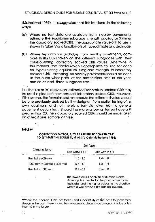
(a) Where no test data are available from nearby pavements. estimate the equilibrium subgrade strength as a factor (F) times the laboratory soaked CBR. The appropriate value of F to use is shown In Table IVas a function of soli type. climate and drainage.
(b) Where test ddta are dvdllable tram nearby povements. compare In situ CBRs taken on the different subgrades with their corresponding laboratory soaked CBR values. Determine in this manner the faefor which is appropriate to use for each soli type relating equilibrium subgrade strength to laboratory soaked CBR. All testing on nearby pavements should be done In the outer wheelpath. at the most critical time of the year. and on at least three subgrade sites.
Ih either (0) or (b) above. an 'estimated' laboratory soaked CBR may be used In place of the measured laboratory soaked CBR. However. If this is done. the formula used to computethe estimated value should be one previously derived by the designer from earlier testing of his own local salls. and not merely a formula taken from a general pavement design text. Should the material being tested have a PI greater than 20. then laboratory soaked CBRs should be undertaken on at least one sample in three.
tABLE Iv CORRECTION FACTOR, F, TO BE APPLIED TO SOAKED CBR'
TO ESTIMATE THE EQUILIBRIUM IN SITU CBR (Mulhollond 1986)
Climatic Zone
Rainfall ~ 600 mm
1000 mm ~ Rainfall> 600 mm
Rainfall> 1000 mm
Soil Type
Salls with PI < 11
1.0- 1.5
0.6 - 1.1
0.4- 0.9
SOilS with PI > 11
1.4 - 1.8
1.0 - 1.4
0.6 - 1.0
The lower values apply to a situation where drainage is expected to be poor. water table high. etc. and the higher values to the situation where a well drained site can be assured.
'Where the soaked CBR has been used successfully as the basis for pavement design In the past. there should be no reason to discontinue using on F value of less than 1.0 In the future.
12 . ARR[) SR 41. 1989
STRUCTURAL DESIGN GUIDE FOR FLEXIBLE RESIDENTIAL STREET PAVEMENTS
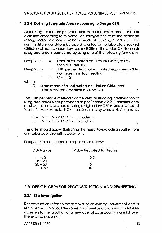
2.2.4 Defining Subgrade Areas According to Design CBR
At this stage in the design procedure. each subgrade area has been classified according to its particular soil type and assessed drainage rating; and predictions have been made of Its strength under equilibrium moisture conditions by applying a factor to laboratory soaked CBRs (or estimated laboratory soaked CBRs). The design CBR for each subgrade area Is computed by using one of the following formulae:
Design CBR Least of estimated equilibrium CBRs (for less than five results).
Design CBR 10th percentile of all estimated equilibrium CBRs (for more than four results). C - 1.3 S
where C Is the mean of all estimated equilibrium CBRs. and S is the standard deviation of all values.
The 10th percentile method can be very misleading If deilneation of subgrade areas is not performed as per Section 2.2.2. Particular care must be taken to exclude any single high or low CBR result. a so-called 'outlier'. For example. if CBR results on a clay were 5. 4.7.8 and 15:
C - 1.3 S = 2.2 if CBR 15 is included. or C - 1.3 S = 3.6 if CBR 15 is excluded.
The latter should apply. illustrating the need to exclude an outlier from any subgrade strength assessment.
Design CBRs should then be reported as follows:
CBR Range
<5 5-20
20-50 >50
Value Reported to Nearest
0.5 1 5
10
2.3 DESIGN CBRs FOR RECONSTRUCTION AND RESHEETING
2.3.1 Site Investigation
Reconstruction refers to the removal of an existing pavement and its replacement to about the same finanevel and alignment. Resheeting refers to the addition of a new layer of base quality material over the existing pavement.
ARRB SR 41. 1989 13
STRUCTURAL DESIGN GUIDE FOR FLEXIBLE RESIDENTIAL STREET PAVEMENTS
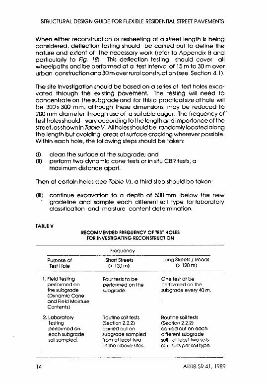
When either reconstruction or resheeting of a street length is being considered. deflection testing should be carried out to define the nature and extent of the necessary work (refer to Appendix Band particularly to Fig. 18). This deflection testing should cover all wheel paths and be performed at a test InteNal of 15 m to 30 mover urban construction and 30 m over rural construction (see Section 4.1).
The site Investigation should be based on a series of test holes excavated through the existing Pdvement. The testing Will need to concentrate on the subgrade and for this a practical size of hole will be 300 x 300 mm. although these dimensions may be reduced to 200 mm diameter through use of a suitable auger. The frequency of test holes should vary according to the length and importance of the street. as shown In Table V. All holes should be randomly located along the length but avoiding areas of surface cracking wherever possible. Within each hole. the following steps should be taken:
(I) clean the surface of the sub grade: and (II) perform two dynamic cone tests or In situ CBR tests. a
maximum distance apart.
Then at certain holes (see Table \/). a third step should be taken:
(iii) continue excavation to a depth of 500 mm below the new gradeline and sample each dltterent soil type tor laboratory classification and moisture content determination.
TABLE V
14
RECOMMENDED FREQUENCY OF TEST HOLES FOR INVESTIGATING RECONSTRUCTION
Purpose of Test Hole
1. Field Testing performed ()n the subgrade (Dynamic Cone and Field Moisture Contents)
2. Laboratory Testing performed on each subgrade soli sampled.
Frequency
Short Streets « 120 m)
Four tests to be performed on the subgrade.
Routine soil tests (Section 2.2.2) carned out on subgrade sampled from at least two of the above sites.
Long Streets / Roads (> 120 m)
One test ot be performed ()n the subgrade every 40 m.
Routine soil tests (Section 2.2.2) carned out on each different subgrade soil - at least two sets of results per soil type.
ARRO SR 41. 1989
STRUCTURAL DESIGN GUIDE FOR FLEXIBLE RESIDENTIAL STREET PAVEMENTS
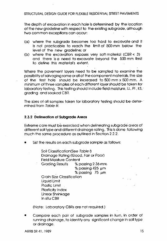
The depth of excavation in each hole is determined by the location of the new gradeline with respect to the existing subgrade. although two common exceptions can occur:
(a) where the subgrade becomes too hard to excavate and It is not practicable to reach the limit of 500 mm below the level of the new gradeline: or
(b) where the excavation exposes very soft material (CBR < 3) and there is a need to excavate beyond the 500 mm limit to define this material's extent.
Where the pavement layers need to be sampled to examine the possibility of salvaging some or all of the component materials. the size of the test hole should be increased to 500 mm x 500 mm. A minimum of three samples of each different layer should be taken for laboratory testing. This testing should include field moisture. LL. PI . LS. grading and soaked CBR.
The sizes of all samples taken for laboratory testing should be determined from Table fIf.
2.3.2 Delineation of Subgrade Areas
Extreme care must be exercised when delineating subgrade areas of different soil type and different drainage rating. This Is done following much the same procedure as outlined in Section 2.2.2.
• List the results on each subgrade sample as follows:
Soil Classification(See Table /) Drainage Rating (Good. Fair or Poor) Field Moisture Content Grading Results "10 passing 2.36 mm
"10 passing 425 11m "10 passing 75 11m
Grain Size Classification Liquid Limit Plastic Limit Plasticity Index Linear Shrinkage In situ CBR
(Note: Laboratory CBRs are not required.)
• Compare each pair of subgrade samples in turn. In order of running chainage. to identify any significant change in soli type or drainage.
ARRB SR 41. 1989 15
STRUCTURAL DESIGN GUIDE FOR FLEXIBLE RESIDENTIAL STREET PAVEMENTS
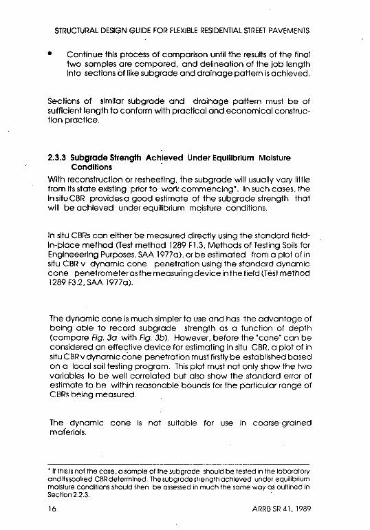
• Continue this process of comparison until the results of the final two samples are compared. and delineation of the job length Into sections of like subgrade and drainage pattern is achieved.
Sections of similar subgrade and drainage pattern must be of sufficient length to conform with practical and economical construction practice.
2.3.3 Subgrade Strength Achieved Under Equilibrium Moisture Conditions .
With reconstruction or resheeting. the subgrade will usually vary little from Its state existing prior to work commencing". In such cases. the In situ CBR provides a good estimate of the subgrade strength that will be achieved under equilibrium moisture conditions.
In situ CBRs can either be measured directly using the standard fieldIn-pldce method (Test method 1289 F 1.3. Methods of Testing Soils for Englneeering Purposes. SAA 1977a). or be estimated from a plot of in situ CBR v dynamic cone penetration using the standard dynamic cone penetrometer as the measuring device in the field (Test method 1289 F3.2. SAA 1977a).
The dynamic cone is much simpler to use and has the advantage of being able to record subgrade strength as a function of depth (compare Fig. 30 with Fig. 3b). However. before the 'cone' can be considered an effective device for estimating in situ CBR. a plot of in situ CBR v dynamic c·one penetration must firstly be established based on a local soil testing program. This plot must not only show the two variables to be well correlated but also show the standard error of estimate to be within reasonable bounds for the particular range of CBRs bp.ing measured.
The . dynamic cone Is not suitable for use In coarse-grained maferials .
• If this Is not the case. a sample of the subgrade should be tested in the laboratory and its.soaked CBR determined. The subgrade strength achieved under equilibrium moisture conditions should then be assessed in much the some way as outlined in Section 2.2.3.
16 ARRB SR 41. 1989

STRUCTURAL DESIGN GUIDE FOR FLEXIBLE RESIDENTIAL STREET PAVEMENTS
Fig. 3a - Pictorial view of the dynamic cone penetrometer
Fig. 3b - Pictorial view of the in situ CBR apparatus
2.3.4 Defining Subgrade Areas According to Design CBR
In the case of reconstruction or resheeting, the assessment of design CBR is reasonably straightforward: one ar other of the following equations should be used for each different subgrade area:
Design CBR
Design CBR
where:
least of estimated equilibrium CBRs (for less than five results) 10th percentile of all estimated equilibrium CBRs (for more than four results) C -1.3 S
C Is the mean of all estimated equilibrium CBRs, and S is the standard deviation of all values.
ARRB SR 41, 1989 17

STRUCTURAL DESIGN GUIDE FOR FLEXIBLE RESIDENTIAL STREET PAVEMENTS
Estimated equilibrium CBRs are usually made equal to the estimated in situ CBRs (see Section 2.3:3). In the case where the design CBR is computed as the 10th percentile of all estimated equilibrium CBRs, any 'outliers' must firstly be eliminated from the computation (see Section 2.2.4).
2.4 DRAINAGE CONSIDERATIONS
2.4.1 Drainage Factors Affecting Design
Drainage and its effect on pavement performance should be considered from two different but rEllated viewpoints.
Firstly, a best estimate Is made of how drqinoge will affect the 'equilibrium' strength ofthe subgrade. Section 2.2.3 of the Guide Indicates the way in which this should be done. by estimating the equilibrium subgrade CBR dependent upon subgrade material type, clitT'late and drainage conditions expected to exist at the site.
Secondly, steps should be taken to Improve any poor drainage currently existing at the site. The nature of the terrain and the rainfall paffern at the site will both be critical factors to consider.
Poorly drained pavements are most offen associated with:
• sites in flat or gently-undulating country; • sites where a shallow water table exists; • sites where irrigation or excessive garden watering occurs; • sites where active springs or aquifers exist; • sites which are known to be subject to flOOding: and/or • high rainfall.
For new construction. therefore. the soil sUNey should include the location of any springs, zones of seepage or water-bearing strata. When subsurface water is encountered during investigatory drilling, the borehole(s) should be cased so that the maximum height of the water table can be determined.
In the case of reconstruction, particular attention should be directed to assessing the moisture conditions existing within the old pavement and the subgrade. and to gauging the effectiveness of the various elements of the existing drainage system. Areas of surface cracking are natural locations where moisture will tend to congregate In pavement layers and/or the subgrade. Site evaluation should include therefore making a comparison of field moisture contents with respective plastic limits or optimum moisture content values. Should field
18 ARRB SR 41. 1989
.1'

STRUCTURAL DESIGN GUIDE FOR FLEXIBLE RESIDENTIAL STREET PAVEMENTS
moisture contents of subgrade samples exceed plastic limits or optimum moisture contents by 10 per cent. this would indicate that the subgrade will need drying out during construction. Also. notes should be taken describing the condition of kerb and channels. the type. width and condition of pavement surfacing. pavement crossfall. and the effectiveness of any subsurface drains present (I.e. whether they are still working or not).
2.4.2 Drainage Factors Affecting Construction
For new streets the aim should be to construct the pavement as far above the water table as practically or economically possible. The minimum difference between the subgrade and the level of the water table should be 600 mm. If a pavement cannot be built to meet this requirement. consideration shoulci be given to the installation of subsurface drains to lower the water table by the required amount.
Drainage problems are often encountered where a high water table Is found to exist adjacent to a cutting. particularly where the original water table is at a higher elevation than the pavement 5urfoce. In such situations. provision of subsurface drains must always be considered.
On flat or gently-sloping ground. strict level control should be maintained during the construction process. Subsurface drains along the lower edge of the pavement may also be warranted in these circumstances.
The following guidelines apply to overall pavement drainage. given the availability of suitable pavement materials;
(a) No pavement layer should be entirely surrounded by materials of lower permeability (see Fig.4a).
(b) The flow path to the subsurface drain should proceed through materials of increasing permeability (see two alternatives in Figs 4b and 4c).
(c) The capacity of the subsurface drainage system should be adequate to dispose of estimated quantities of water from surface infiltration ar other sources. Gerke (1987) provides a comprehensive guide to the design of subsurface drainage systems.
Other factors required to maintain good drainage are:
• regular observations to be made of the drainage system after periods of prolonged rainfall. .
• quick action to be taken to flush out blocked subsurface drains and to clean blocked outlet structures.
ARRB SR 41. 1989 19

STRUCTURAL DESIGN GUIDE FOR FLEXIBLE RESIDENTIAL STREET PAVEMENTS
Fig. 40 - Unsatisfactory subsurface drain arrangement: water from the basecourse is unable to reach the subsurface
drain through the subbase
I more permeable I than base I I I . I 0 I Alternative drain l. - __ .. placement
Fig. 4b - Satisfaction subsurface drain arrangement: water from the basecourse is able to reach the subsurface drain through
20
the subbase
Fig. 4c - Alternative satisfactory subsurface drain arrangement to Fig. 4b: water from the basecourse Is given direct
access to the subsurface
ARRB SR 41. 1989

STRUCTURAL DESIGN GUIDE FOR FLEXIBLE RESIDENTIAL STREET PAVEMENTS
• pothole repair and sealing of cracks in an exi~ting pavement to be an Integral part of any maintenance program to minimise moisture infiltration.
Finally. care should be taken in the selection of trees and/or shrubs to be planted close to any street pavement. Some types of vegetation will cause drying out of the subgrade which. in expansive clays leads to significant distortion of the pavement surface (Mcinnes 1986 and Barry 1986). These two references outline the problem. provide a list of suitable shrubs and trees. and specify planting clearances.
ARRB SR 41. 1989 21
3. THE NATURE AND LEVEL OF TRAFFIC LOADING
3,1 GENERAL
The performance of the residential street pavement is affected by the nature and level of traffic loading encountered over its design life. In this Design Guide, for the purposes of determining the composite effect of traffic, two major assumptions are made.
The first assumption concerns the means of computing load equivalents between different axle configurations. For this, standard axle loads need to be Identified for the various configurations. Such standard axle loads are set by regulation:
• for a single axle consisting of single tyres, the standard load = 5.4 t,
• for a single axle consisting of dual tyres, the standard load = 8.2 t, and .
• for a tandem axle consisting of dual tyres, the standard load = 13.6 t.
These loads are considered to be equivalent because they produce the same maximum surface deflection and each is assumed to cause approximately the same damage to a pavement. One pasS of a standard load is taken to be an equivalent standard axle (ESA).
The second assumption concerns the me<;lns of computing equivdlent standard axles for a particular axle configuration carrying other than its standard load. It is assumed here that the 'fourth power law' applies. The application of this law means that an axle or axle group of load P and standard load Ps has as much damaging effect on a pavement as (P/PS)4 equivalent standard axles (ESA).
The composite effect of a traffic stream consisting of different axie types and loads can therefore be found by converting all axle passes to ESA and determining the total. The Design Traffic Value is then the total number of ESA occurring over the design life of the pavement.
22 .A.RRB SR 111; 1989
STRUCTURAL DESIGN GUIDE FOR FLEXIBLE RESIDENTIAL STREET PAVEMENTS
The following Sections Indicate, step by step, how to compute the Design Traffic Value taking Into account:
• present ar predicted commercial traffic volumes, • commercial traffic growth, • street capacity, and • design life of pavement.
Two sepdrdte cases are treated herein:
(a) new construction (Section 3.2); and (b) reconstruction and resheetlng (Section 3.3).
3.2 DESIGN TRAFFIC VALUE FOR NEW CONSTRUCTION
3.2.1 Construction Traffic
Construction fraffic Is brought on by the construction of new houses during the staging of a SUbdivision. During this staging, each completed pavement must take its share of the total number of construction traffic movements generated. The usual assumption made is thot construction traffic can be equated to:
(Number of houses seNlced by the street) x (Number of ESA generated by the average house)
Various figures are quoted in relation to the number of ESA generated by the construction of the average housing residence: 16 ESA (Drew 1981) through to 24 ESA (Schofield 1985). Construction traffic caused by the later installation of in-ground swimming pools, etc. should also be considered. In the absence of evidence of a need for special calculations, it Is recommended that a value of 20 ESA per residence be adopted.
The number of residences seNiced by each street is not always easily determined, particularly where streets are set out in a grid system, because of the many pOints of access. Traffic studies have shown that traffic generated in residential streets varies between 4 and 12 trips per day per residence (Schofield, Mulholland and Morris 1984). By' assuming a number of vehicle trips per day per residence, an estimate of the number of dwellings seNlced by each street can be made from the annual average daily traffic (AADT). By adopting a figure of seven vehicle trips per day per residence, the following equation can be used to predict construction traffic:
Construction traffic ESAs = (AADT /7) x 20 = 3 AADT
ARRB SR 41. 1989 23

STRUCTURAL DESiGN GUIDE FOR FLEXIBLE RESIDENTIAL STREET PAVEMENTS
The sta~ing of the subdivision will determine the number of days over which the construction traffic will apply. . . ,
3.2.2 In-service Traffic
In-service traffic takes into account all traffic other than construction vehicles, buses and garbage services. In-service traffic Is giver, uy 1I1~ tollowing general forrnulu:
In-service traffic ESAs = Ns ' 365. Y
where: . N ESA per day per lane for commercial vehicles other
than buses'and garbage vehicles s
Y p for r = 0
( I + r)P - 1 Y for r > 0 ahd Q = P'
In(l+r)
( 1 + r)Q - 1 y + (P - Q) ( 1 +r )Q-l
In(l+r) for r > 0 and Q < P
traffic growth rate
P design life in years
Q time In years for traffic to reach saturation level.
The three basic variables which influence In-service traffic are N r and P, which are now discussed in more detail. s.
N s. can be arrived at either by adopting an ESA value from Table VII or by using the AADT, percentage commercial vehicles (% CV) and ESA/CV figures given in Table VII and calculating Ns as: '
AADT <>foCV N = -- x x ESA ICV
s 2 100
For streets expected to take industrial trafficking, computations should be done using figures approaching the higher values in the table. Allowance must also be made for
"See TobIe VI for values of Y as a function of P and r
24 Ar~RB SR 41. 1989

STRUCTURAL DESIGN GUIDE FOR FLEXIBLE RESIDENTIAL STREET PAVEMENTS
double trafficking In the case of narrow pavements having widths less than 5.0 m or In the case of pavements having widths less than 9.0 m with consistent levels of kerbside parking.
r: Is usually dependent on the level of traffic. If traffic increases cannot be predicted, an appropriate value taken from ' Table VII should be adopted.
P: may need to be adjusted to take into account the bUild-up In traffic In the early years of subdivision construction. Collectors and distributors in particular would take some time (between five and ten years) to service all traffic generated from adjacent subdivisions. It would be expected that traffic on these Joads would start at a zero level and build up to a nedr maximum over the five to ten-year period, For traffic cdlculation, therefore, P should be reduced effectively by one-half of the assumed build-up period.
TABLE VI VALUES OF tHE GiloWtk FACTOR Y AS A FUNCTION OF P and r.
~I 5 10 15 20 25 30 35 40
0.000 5,00 10.00 15,00 20,00 25,00 30,00 35,00 40,00
0.005 5,06 10,24 15,57 21.02 26,61 32,36 38,22 44,25
0,010 5,13 10,51 16,18 22.13 28,38 34.95 41.87 .49,14
0.Ql5 5.19 10.78 16,80 23,29 30,28 37,82 45,93 54,65
0,020 5.26 11,06 17,47 24,55 32,35 40,98 SO,50 61,03
0.Q25 532 11,34 18,15 25,85 34,57 44,48 55,60 68,21
0,030 5.39 11,63 18,88 27,28 37.00 48,28 61.36 76,54
3.2.3 Bus Traffic
The formula for estimating bus trdffic is as follows:
Bus traffic ESAs = N b' 365. Y
where:
N = bus L (no. of services/day/lane x ESA per b types bus)
ARRB SR 41. 1989 25

STRUCTURAL DESIGN' GUIDE FOR FLEXIBLE RESIDENTIAL STREET PAVEMENTS
Y = as defined previously for in-service traffic. (This assumes that bus traffic varies directly with In-service traffic over the design life of the pavement).
To estimate N b requires a study of the planned use of buses by bus type and a determination of the ESA per bus for each bus type. The latter range between 0.6 and 1.4 ESA for light duty buses and 1.3 to 3.7 ESA fui' heavy duty buses.
TABLE VII TRAFFIC STATISTICS FOR RESIDENTIAL STREETS
Updated figures from Mulholland (1986) Figures In bracket~ are mean values.
Street Type AADT %CV ESA I CV ESA I Day Limits Per Lane
Minor <150 1.0- 15.0 0.01- 0.70 0.03 - 5.0 0.00 (3.6) (0.20) (0.40)
Local Access 150- 1000 1.0 - 25.0 0.10- 1.00 0.2- 15 0.01 (5.0) (0.50) (4.0)
Collectors 1000- 3000 2.0- 20.0 0.10 - 1.20 5-90 0.015 o.m (0.50) (30)
Dstributors >3000 2.0- B.O 0.20 - 0.90 20-190 0.Q25 (3.7) (0.50) (60)
3.2.4 Garbage Traffic
Two principal assumptions are made in estimating garbage traffic In terms of ESA. It is assumed that:
(i) garbage traffic will remain reasonably constant over the design life of the pavement; and
(ii) garbage trucks in local access and minor streets will traffic the outer wheel path only 50 per cent of the time.
Garbage traffic is then estimated according to:
Garbage traffic ESAs = Ng
• 52. P
where: N
g = ESA per garb,age truck x no. of passes per week x f
'26 ARRB SR 1.11, 1989

STRUCTURAL DESIGN GUIDE FOR FLEXIBLE RESIDENTIAL STREET PAVEMENTS
proportion of the time garbage trucks traffic the outer wheel path 0.5 for minor and local access streets 1.0 for collectors and distributors.
A two-axle garbage truck has an average loading of 2.14 ESA and a three-axle garbage truck has a value of 3.04 ESA (Schofield 1985). If the loading is not known, an appropriate value to use would be 2.6 ESA.
3.2.5 The Design Life In Terms of ESA
The Design Life In years (P) should only be specified after a cost study has been made of different design-maintenance options. Nevertheless, it Is common practice to adopt:
20 years < P < 40 years for urban (fixed level) construction; and
10 years < P < 30 years for rural (non-fixed level) construction,
It may be necessary to adjust the P value to take into account the build-up in traffic in the early years of subdivision traffic (refer to the note regarding P given in Section 3,2.2),
Using an appropriate value for p, the Design Traffic Value can be computed in terms of ESA as the sum total of:
• Construction traffic ESAs, • In-service traffic ESAs, • Bus traffic ESAs, and • Garbage traffic ESAs,
A final check should be mode to ensure that the computed Design Traffic Value is of the right order forthe street type concerned. Table VIII provides a basis for this final check.
TABLE VIII
RANGE OF ES~ FOR A TYPICAL STREET (BASED ON A 20 YEAR DESIGN LIFE)
Street Type
Minor
Local Access
Collector
Distributor
ARRB SR 41, 1989
Range of Computed ESA
2 X 1(}' - 6 X 10'
3X 10' - 3X lOS
6 X 10' - 2 X 1()6
above'3 X 10⁵ •
27

STRUCTURAL DESIGN:GUIDE FOR FLEXIBLE RESIDENTIAL STREET PAVEMENTS
Use the NAASRA pavement design manual (NAASRA 1987)for over 1 ()6
ESA. The street types are defined by the AADT limits given In Table VII.
3.3 DESIGN TRAFFIC VALUE FOR RECONSTRUCTION AND RESHEETING
3.3.1 Traff!c COI_lnt Prpcedure
The traffic count procedure defined below assumes Ihat little trdfflc loading data are available for the pavement to be reconstructed or resheeted and that no weigh-in-motion devices are available.
The steps to be taken to acquire traffic loading data from a one-day manual count of commercial vehicles by number and load distribution follow.
Step 1 Establish a set of vehicle configurations by which the person counting can clearly distinguish the different vehicle types by axle arrangements. A useful set is shown in Fig. 5.
Step 2 Classify each vehicle by estimated per cent fully loaded.
Where there is no indication of the load within an enclosed truck. assume 50 per cent laden.
Step 3 Record the number of commercial vehicles each hour in both directions during the count and classify each cammer cial vehicle according to vehicle type and estimated per cent loading. A proforma such as that shown in Fig. 6 should suffice forth is purpose. Hours at recording could probably be restricted to 8 hours. 7.00 a.m. to 11.00 a.m. and 2.00 p.m. to 6.00 p.m .. to cover batt) peak periods during the day.
The results from the one day manual count should be summarised thus:
TABLE IX
COMMERCIAL VEHICLE COUNT BY VEHICLE TYPE AND ESTIMATED'. LOADING
Light Truck Two Axle Three Axle Articulated or Van Heavy Truck Heavy Truck Vehicle Buses
• E 25 50 75 F E 25 50 75 F E 25 50 75 F E 25 50 75 F E 50 F
Totals overS 2. hours
3 3 2 1 2
(Sample values only)
• E = Empty . 25 = 25 per cent laden 75 = 75 per cent laden
28
2
50 = 50 per cent laden . F = Full:
ARRB SR 41. 1989

STRUCTURAL DESIGN GUIDE FOR FLEXIBLE RESIDENTIAL STREET PAVEMENTS
TARE IT}
T<3
Tare ·Net Gross
GVM
II 3<T<6 ---
Tare Net Gross
GVM
III T>6
Tare Net
Gross GVM
DESCRIPTION
RIGID TRUCK: light two axle truck with dual rear wheels
~ 0 J 1.0 1.0 1.0 1.5 2.0 2.5
4.5 t
RIGID TRUCK: Heavy two axle trucks with dual rear wheels used by councils or carriers of goods
~I I (0 0 J
3.5 2.5 1.9 6.0 5.4 8.5
14 t
RIGID TRUCK: Three <lxle highway trucks used by quarries or highway carriers .
J5i1 I ·~....L.-f-'--_-_----'0=-o _----::::;:0:-r'J
3.5 1.9 5.4
20 t
. 3.5
11.5 15.0
'.1 .
Fig 5 - Set of vehicle configurations to be used in manual traffic IOdding count G"vM = gross vehicle mass; T = tare mass
ARRB SR 41. 1989
.\."!" . • .. \',
~1'
:.1
.-
29

STRUCTURAL DESIGN GUIDE FOR FLEXIBLE RESIDENTIAL STREET PAVEMENTS
IV SEMI-TRAILER' Any heavy articulated vehicle, . ""~""5 axle configuration assumed
v
..
. '.~ "
~C::::::::0=G~o ·'\.==-~==-~=0===-=0~J '. ./
Tare 4.0 4.0 Net .0 11.0 Gross 4.0 15.0 GVM 34t
. BUS Any heavy duty bus
es Tare 4.0 Net 2.5 Gross 6.5
GVM 15 t \
4.0 11.0 15.0
1{5U 1.0 i.5 8.6
Fig 5 (Cont).- Set of vehicle configurations +0 be used in manual traffic loading count GVM = gross vehicle mass; T = tare mass
Desirably, three days of such counts should be recorded, say on a Monday, aWednesday and a Saturday of a typical working week and these counts should take in at least one day of the garbage collection.
A seven day traffic count by automatic traffic counter would be useful information to have on hand to determine the distribution of traffic over' a week and to estimate the per cent CV for the street under examination.
.30 . ARRB SR 41. 1989

» ;;::) ;;::) OJ (J) ;;::)
J:>. :-'
-0 ex> -0
-n <6. 0-
6 =l: o· () 0 C :l -+ U a 0' 3 Q
ARRB Residential Street Traffic Survey ARRB PROJECT NO. 392 : Design and Maintenance of Residential Streets
Name of Street: Location: Suburb : Width of Pavement (m) . Date . Estimated No of Allotments Serviced .
Vehicle (CVt,re) T<3 3$ T < 5 n5 Semi-trailers Buses type Non·CV (cars) (CVne1) 2.5 8.0 13.5 22.0 4.0 Comments •
lime E 25 50 75 F E 25 50 75 F E 25 50 75 F E 255075 F E 50 F
Total
Note: Traffic shall be counted In both directions • Special note shall be taken of whether CVs share IWPs.
~ ;;::) C q C
~ ,-CJ m (J)
G) Z (J) c a m
o ;;::)
-n ,-m X 55 ,-m ;;::)
rn o m Z -I }> ,-
~ ;;::) m m -I
~ m ~ m Z uJ
STRUCTURAL DESIGN GUIDE FOR FLEXIBLE RESIDENTIAL STREET PAVEMENTS
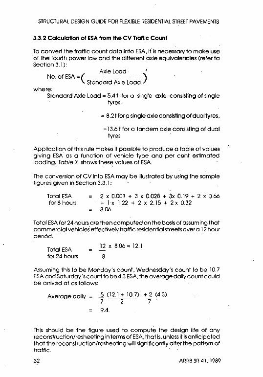
3.3.2 Calculation of ESA from the CV Traffic Count
To convert the traffic count data into ESA. If Is necessary to make use of the fourth power law and the different axle equivalencies (refer to Section 3.1):
Axle Load 4
No. of ESA =( ) Standard Axle Load
where: Standard Axle Load =5.4 t for a single axle conslstihg of single
tyres.
= 8.2 Hor q single' axle consisting of dualtyres.
= 13.6 t for a tandem axle consisting of dual tyres.
Application of this rule makes it possible to produce a table of values giving EsA as a function of vehicle type and per cent estimated loading: Table X shows these values of ESA.
The conversion of CV into ESA may be illustrated by using the sample figures given in Section 3.3.1:
Total ESA for 8 hours
2 x 0.001 + 3 x 0.b28 + 3x 0.19 + 2 x 0.66 . + lx 1.22 + 2 x 2.15 + 2 x 0.32
8.06
Total ESA for 24 hours are then computed on the basis of assuming that commercial vehicles effectively traffic residential streets over a 12 hour period.
Total ESA for 24 hours
12 x 8.06 = 12.1
8
Assuming this to be Monday's count. Wednesday's count to be 10.7 ESA and Saturday's count to be 4.3 ESA. the average daily count could be arrived at as follows:
Average daily = ...§. (12.1 + 10.7) +-.1, (4.3) 7 2 7 9.4.
This should be the figure used to compute the design life of any reconstruction/resheeting in terms of ESA. that is. unless it is anticipated that the reconstruction/resheeting will significantly alter the pattern of traffic.
32 ARRB SR 41. 1989

STRUCTURAL DESIGN GUIDE FOR FLEXIBLE RESIDENTIAL STREET PAVEMENTS
TABLE X
ESA AS A FUNCTION OF VEHICLE TYPE AND PER CENT LOADING (Schofield 1985)
Truck Load Light Two Axle Three Axle Articulated Large Truck Heavy Heavy Vehicle Buses
Truck Truck
Tare (t) T<3 3~T<5 T~5 Sflmis Ruses Net (t) N = 2.5 N =8.0 N = 13.0 N = 22.0 N =4.0
E 0.001 0.19 0.18 0.32 0.83 25% 0.004 0.35 0.34 0.42 50% 0.008 0.66 0.67 0.78 1.73 75% 0.016 1.22 1.33 1.62 F 0.Q28 2.15 2.48 3.26 3.21
3.3.3 beslgn life In terms of ESA
the adopted design life In years (P) is converted to total ESA by use of the following formula:
Design Traffic Value = (Average Daily ESA Count) x 365 x y
where: y=
y=
y=
P for r = 0
In(l+r)
In (1 +r)
for r > 0 dnd Q = P'
+(P-Q)( 1 +r)Q-l
for r > 0 and Q < P
r = traffic growlh role (refer Table VI)
P = design life in years
Q = time in years, for traffic to reach saturation level.
Any future traffic increases expected over and above those given by the value r should be allowed for by reference to Section 3.2.3 (for buses) and/or to Section 3.2.4 (for garbage services). .
'(See Tobie VI for values)
ARRB SR 41, 1989 33
:;,
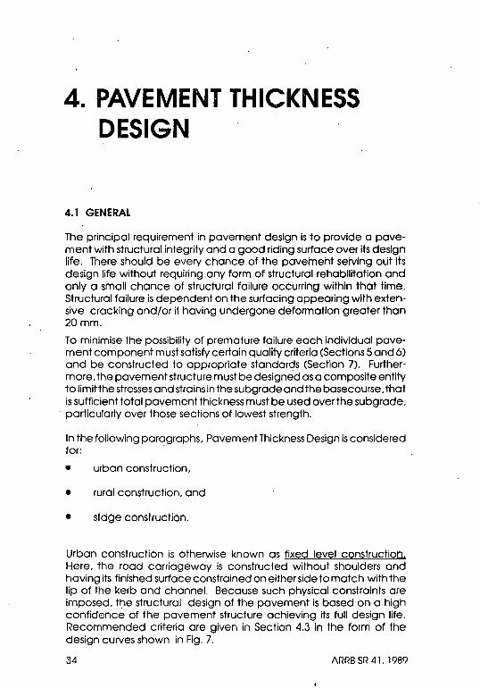
4. PAVEMENT THICKNESS DESIGN
4.1 GENERAL
The principal requirement in pavement design is to provide a pavement with structural integrity and a good riding surface over its design life. There should be every chance of the paveinent serving oLit its design life without requiring any form of structural rehabilitation and only a small chance of structural failure occurring within that time. Structural failure Is dependent on the surfacing appearing with extensive cracking and/or it having undergone deformation greater than 20mm.
To minimise the possibility of premature failure each individual pavement component must satisfy certain quality criteria (Sections 5 and 6) and be constructed to appropriate standards (Section 7). Furthermore, the pavement structure must be designed as a composite entity to limit the stresses and strains in the subgrade and the basecourse, that is sufficient total pavement thickness must be used over the subgrade, particularly over those sections of lowest strength.
In the following paragraphs, Pavement Thickness Design is considered for: .
• urban construction,
• rural construction, and
• stage construction.
Urban construction is otherwise known as fixed level construction. Here, the road carriageway is constructed without shoulders and having its finished surface constrained on either side to match with the lip of the kerb and channel. Because such physical constraints are imposed, tt'le structural design of the pavement is based on a high confidence of the pavement structure achieving its full design life. Recommended criteria are given in Section 4.3 in the form of the design CUNes shown in Fig. 7.
34 ARRB SR 41, 1989
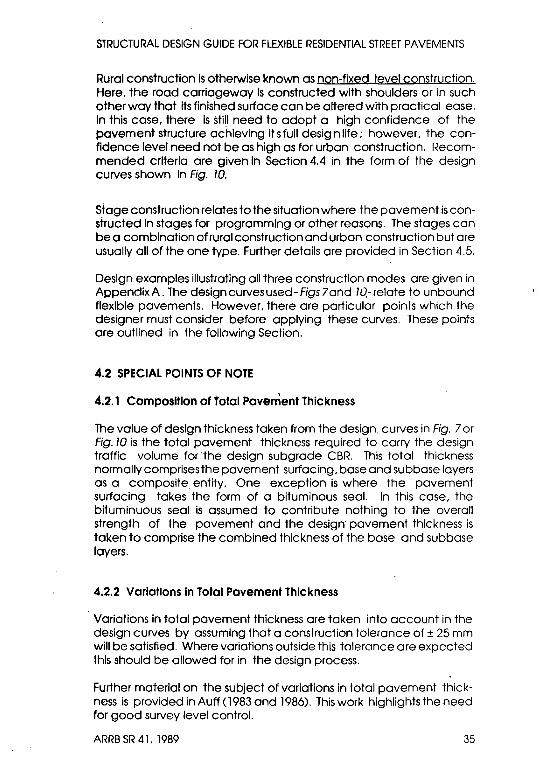
STRUCTURAL DESIGN GUIDE FOR FLEXIBLE RESIDENTIAL STREET PAVEMENTS
Rural construction Is otherwise known as non-fixed level construction. Here. the road carriageway Is constructed with shoulders or in such other way that Its finished surface can be altered with practical ease. In this case. there is still need to adopt a high confidence of the pavement structure achieving Itsfull designlife: however. the confidence level need not be as high as for urban construction. Recommended criteria are given In Section 4.4 in the form of the design CUNes shown In Fig. 10.
stage construction relates to the situation where the pavement is constructed In stages for programming or other reasons. The stages can. be a combination of rural construction and urban construction but are usually all of the one type. Further details are provided in Section 4.5.
Design examples illustrating all three construction modes are given in Appendix A. The design CUNes used - Figs 7 and 10,- relate to unbound flexible pavements. However. there are particular points which the designer must consider before applying these CUNes. These points are outlined in the following Section.
4.2 SPECIAL POINTS OF NOTE
4.2.1 Composition of total Pavement Thickness
The value of design thickness taken from the design CUNes in Fig. 7 or Fig. 10 is the total pavement thickness required to carry the design traffic volume for the design subgrade CBR. This total thickness normally comprises the pavement surfacing. base and subbase layers as a composite entity. One exception is where the pavement surfacing takes the form of a bituminous seal. In this case. the bituminuous seal is assumed to contribute nothing to the overall strength of the pavement and the design' pavement thickness is taken to comprise the combined thickness of the base and subbase layers.
4.2.2 Variations in Total Pavement Thickness
Variations In total pavement thickness are taken Into account in the design CUNes by assuming that a construction tolerance of ± 25 mm will be satisfied. Where variations outside this tolerance are expected Ihls should be allowed for in the design process.
Further material on the subject of variations in total pavement thickness is provided in Auff (1983 and 1986). This work highlights the need for good sUNey level control.
ARRB SR 41. 1989 35

STRUCTURAL DESIGN GUIDE FOR FLEXIBLE RESIDENTIAL STREET PAVEMENTS
4.2.3 Thickness of Pavement Components
For practical reasons it is recommended that the following minimum layer thicknesses be adopted:
MlnlmLim Thickness
Asphull SUi'faclng 25mm
Bose Loyer l00mm
Subbase Layer l00mm
The total pavement thickness is computed from Fig. 7 or Fig. /0, as appropriate, to provide adequate cover over the subgrade. The thir:-knASS nf basecourse plus asphalt surfacing is computed In similar manner to provide adequate cover over the subbase. Fur this, the design CBR of the subbase is usually assumed to be, 30 (see Sectloh 5.3).
4.2.4 Deflection Check oil Fatigue Cracking
For pavements with a design traffic value greater than lOS ESA, a deflection check is incorporated in the thickness design procedure with the intent of precluding fatigue crocking in the asphalt surfacing. Details of this deflection check can be found in Section 2.2 of the NAASRA Interim Guide to Pavement Thickness Design (NAASRA 1979). The deflection check is Illustrated In Appendix A.l, Worked Example No.2.
It i:; anticipated that this rleflection check will be developed further as research continues to improve the criteria for evaluating pavement structural integrity (see Appendix B). There may be a need to consider setting a limit on surface curvature as well as setting a limit on total surface deflection. Future revisions of the NAASRA Guide will advise of such changes.
4.2.5 Design of Bound Pavements
Where Figs 7 and Ware applied to the design of bound pavemehts, the designer may conservatively assume thu I the bound matericils are equivalent to the unbound materials, unless he has sufficient confidence to apply pavement layer equivalency factors defined by:
Equivalent thickness of unbound material = Equivalency Factor x Thickness of bound material
Preferably, equivalency factors should be established by testing previous construction work or be obtained from some reputable external source.
36 ARRB SR 41. 1989

STRUCTURAL DESIGN GUIDE FOR FLEXIBLE RESIDENTIAL STREET PAVEMENTS
it Is strongly recommended that any bound pavement .qesigned using Fig. 7 or Fig. 10 be checked against the NAASRA Guide to the Structural Design of Road Pavements (NAASRA 1987).
Other design documents may also be referred to:
• the Australian Asphalt Pavement Association's Design Manual (AAPA 1983) - for design of any bitumen-bound pavement.
• the Main Road Department Queensland's Interim Manual for Design of Flexible Pavements (MRD 1981) - for design of any cement-stabilised pavements. (see Section 4.2.6).
• NAASRA's Guide to Stabilisation in Roadworks (NAASRA 1986) - for stabilisation works in general.
4.2.6 Design of Cement-Treated Pavements
Cement is commonly regarded as the most effective additive for treating sand and fine crushed rock, and can also be useful for treating clays when used in combination with lime (NAASRA 1986). The correct proportion of cement to use in any particular situation is best determined by the controlled laboratory testing of specimens of the material containing varying additive concentrations (Dunlop 1980).
The cement treatment of materials for pavement construction can be divided Into two general types:
(a) Cement Modification: in which the cement, up to about 3 per cent by weight of soil, is added to a soil to alter its properties to meet specification requirements.
(b) Cement Stabilisation: in which sufficient cement, commonly between 3 and 10 per cent, is added to a soil to produce a material having usable tensile strength when compacted and cured.
Pavements conSisting of cement-modified materials can be characterised and designed as unbound. However, pavements consisting of cement-stabilised materials must be designed specifically as bound' pavements (see Section 4.2.5 and the following paragraph).
SpeCial precautions should be taken to minimise the risk of shrinkage cracks in the basecourse reflecting through to the wearing surface. For instance, practical difficulties occur with clean well-graded gravels where high strength develops with the addition of cement (Metcalf 1977). A good check is to have samples of the cement-treated material tested in the laboratory to ensure that the seven-day
ARRB SR 41. 1989 37

STRUCTURAL DESIGN GUIDE FOR FLEXIBLE RESIDENTIAL STREET PAVEMENTS
unconfined compressive strength does not rise above 2 MPa. Minimum cover is another Important aspect that should be Investigated (Dunlop 1980 NAASRA 1979). Then for all types of material, careful construction control is essential to achieve thorough mixing. adequate compaction and proper curing (Lay and Metcalf 1983).
Furth!;!r Information on each of these particular points Is available from the Cement and Concrete Association of Australia.
4.2.7 Design of Lime -Treated Pavements
Lime is commonly regarded as the most effective additive for treating clayey soils. and can also be useful for treating plastic quarry materials (NAASRA 1986). The correct proportion of lime to use in any particular situation is best determined by the controlled laboratory testing of !;f)Acimens of the material containing varying additive concentrations (Dunlop 1980).
The lime treatment of materials for pavement construction falls Into the two categories:
(a) Lime Modification whereby small amounts of lime. 1/2 to 1 per cent by weight in the case of granular material and 2 to 3 per cent in the case of clay soils. are added to bring the material to within specification.
(b) Lime stabilisation whereby greater amounts of lime. 2 to 4 per . cent in the case of granular material and 3 to 6 per cent in
the case of soils are added to provide structurally adequate rnotArial for use within the pavement.
Pavements conSisting of lime-modified materials can be chardcterised and designed as unbound. while pavements consisting of IImestabilised materials are best designed on a structural basis utiliSing the tensile strength of the stabilised layer(s) in accordance with NAASRA (1987).
4.2.8 Effect of Vehicle Behaviour
The design curves (Figs 7 and 1(}) take no account of the effect of vehicle behaviour on the performance of a pavement. There are two common cases where vehicle behaviour may be critical:
•
38
Near to or at traffic signals. where it may be necessary to provide stronger and stiffer surfacings to withstand both the stationary loadings and the horizontal forces due to traffic stopping and starting.
ARRB SR 41. 1989
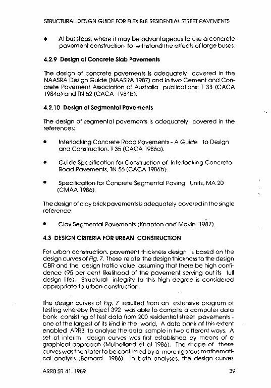
STRUCTURAL DESIGN GUIDE FOR FLEXIBLE RESIDENTIAL STREET PAVEMENTS
• At bus stops. where it may be advantageous to use a concrete pavement construction to withstand the effects of large buses.
4.2.9 Design of Concrete Slab Pavements
The design of concrete pavements is adequately covered in the NAASRA Design Guide (NAASRA 1987) and in two Cement and Concrete Pavement Association of Australia publications: T 33 (CACA 19811a) and TN 52 (CACA 1984b).
4.2.10 Design of Segmental Pavements
The design of segmental pavements is adequately . covered in the references:
• Interlocking Concrete Road Pavement5 - A Guide to Design and Construction. T 35 (CACA 1986a).
• Guide Specification for Construction of Interlocking Concrete Road Pavements, TN 56 (CACA 1986b).
• Specification for Concrete Segmental Paving Units, MA 20 (CMAA 1986).
The design of clay brick pavements is adequately covered in the single reference:
• Clay Segmental Pavements (Knapton and Mavin 1987).
4.3 DESIGN C~ITERIA FOR URBAN CONSTRUCTION
For urban construction, pavement thickness design is based on the design curves of Fig. 7. These relate the design thickness to the design CBR and the design traffic value, assuming that there be high confidence (95 per cent likelihood of the pavement serving out its full design life). Structural integrity to this high degree is considered appropriate to urban construction.
The design curves of Fig. 7 resulted from an extensive program of testing whereby Project 392 was able to compile a computer data bank consisting of test data from 200 residential street pavementsone of the largest of its kind in the world. A data bank of this extent enabled ARRB to analyse the data sample in two different ways. A set of interim design curves was first established by means of a graphical approach (Mulholland et al 1986). The shape of these curves was then later to be confirmed by a more rigorous mathematical analysis (Barnard 1986). In both analyses, the design curves
ARRB SR 41. 1989 39

STRUCTURAL DESIGN GUIDE FOR FLEXIBLE RESIDENTIAL STREET PAVEMENTS
CBR 3D =CBR20
NAASRA Design Curve, indicated bV dashed lines E .s
::l 200 m C -'" -
. 'CBRIS
CBR12-
~~9::'k _
-1r.RA'nJ
ICBRIS)
(~RR1'.1
U
f 300
C Q)
E ~ 400
~
CBR7 ICBR9)
ICBR7) -- ICBRS)
..... ICBR4) 1---. Subgrades with CaR < 3
500 ~ should be designed as per r-- subgrades with CaR = 3 I--- but with the initial subgrade I-- layer stabilised 10 a depth I-- of 100 150 mm
ICBR3)
600L-__ ~ __ ~-L~~LLL-__ ~ __ ~-L~LLLLL-__ -L __ ~~~LLLUL-____ ~ 3456789
103 Hf 3456789
las Trattic: ESA
34567B9
106
Fig. 7 - Interim thickness design curves for residential street pavements, based on a 95 per cent confidence limit
(Mulholland 1986; Barnard 1986)
showed some differences from the NAASRA (1987) design curves within the range of lOS to lO6 ESA and particularly at low CBR values. However, the NAASRA design curves at lOS ESA correspond closely to the rural construction curves of Fig. 10 based on a 90 per cent confid8nGF! (If thF! pavement servinQ out its design life. This Is not unexpected, as the NAASRA curves are based on historical data gathered generally from rural pavements and supported by SRA experience on these pavements.
In addition, factors such as:
• different construction practices and standards
• different traffic patterns,
• different subgrade and drainage conditions, and
• existence of and provision for underground services
support the more conservative design for fixed-level urban streets.
Note: There may be good and valid reasons to vary from the recommended confidence limit of 95 percent. For example, where pave-
40 ARRB SR 41. 1989

';
STRUCTURAL DESIGN GUIDE FOR FLEXIBLE RESIDENTIAL STREET PAVEMENTS
ment materials are scarce or they are particularly costly, the designer has the op,tlon of using a confidence limit of 90 per cent but should not adopt a figure below this for full urban construction. When using a confidence limit of 90 per cent the designer should refer·to the curves of Fig. 10 ..
Three worked examples are given In Appendix A. 1 to illustrate the use of the d.esign method as it applies to urban construction;
• The first example considers the design of a new pavement in a cul- de-sac where design traffic Is less than 105 ESA. Design curves are based on the confidence limit of 90 per cent.
• The second example illustrates the further check that should be made to prevent fatigue cracking occurring in an asphalt surfacing layer which is more than 25 mm thick, and where the design traffic value exceeds 105 ESA. Design curves are based on the confidence limit of 95 per cent
• The third example illustrates the design of an existing local access pavement which is to undergo total reconstruction. Design curves are based on the confidence limit of 95 per cent.
Typical cross-sections for urban construction are shown in Figs 8 and 9.
[k;;&!.K',i:,1.'*'i""';:i'17.Aj;;~;,i:",~~ o 0
Fig.8 - Typical cross-section for an urban pavement with asphaltic concrete surfacing
Fig. 9 - Typical cross-section for an urban pavement with spray and chip seal surfacing
ARRB SR 41. 1989 41'

E
STRUCTURAL DESIGN GUIDE FOR FLEXIBLE RESIDENTIAL STREET PAVEMENTS
4.4 DESIGN CRITERIA FOR RURAL CONSTRUCTION
Much of Section 4.3 applies also to rural construction. The major difference is that pavement thickness design may be based on a highe~ failure probability level because rural construction can accommodate resheeting and asphalt overlays with greater ease than urban comtruction.
·········T·· I' .. __ L .. J .... ,.L·,LI.
MINIMUM BASE THICKNESS
CtnralDOn~!nA NAASRA Design Thicknesses at 106 ESAs
g 200
CBR30 .Q!R20 CBR1S
CBR12
CSl!!
_ ICBR20)
ICBR1S)
ICBR12) ::l Q) C
i-- t-rC8!!!
~ 300 U
CBRS IC~R9)
£ ICBR7)
c Q) 400
..... - ,...... Ir.RRS)
E ~ o a..
..... ICBR4) f--. Subgradcs with CBR < 3
500 ~ should be designed as per f- iuligrlldOI , ... Ith r.RR =:l (CBR3'
E~~Jb~Ut~W£ith~t~h.~;n~ili~'I~'U:~:'.:d'~~~~~~~~~~==~~~~~~~~ __ -=~~ 600
~ laver stabilised to a depth I-- of 100 150 mm
3456789 3456789 3456789
l(f l~ l~ Troffic: ESA
Fig. 10 -Interim thickness design curves for residential steel pavements. based on a 90 per cent confidence limit
(Barnard 1986)
The design curves of Fig. 10 are based on achieving structural integrity to a probability level of 90 per cent (i.e. 10 per cent chance of rehabilitation being required before the end of the design life). These curves have been derived by ARRB using a rigorous statistical analysis of the Project 392 test data (Barnard 1986). Such analysis follows in line with the most recent approaches being adopted by overseas organisations (Lister 1984 AASHTOI Y8S).
A worked example (No.4) is given in Appendix A.2 to Illustrate the outlined design criteria. Because the example assumes a design traffic value of less than 10S ESA. the deflection check for fatigue cracking in the asphalt layer is not carried out (see Worked Example No.2). Typical cross-sections for rural construction are shown in Figs 11 and 12.
42 ARRB SR 41.1989

STRUCTURAL DESIGN GUIDE FOR FLEXIBLE RESIDENTIAL STREET PAVEMENTS
It must be remembered that in using Fig. 70 or any other set of design curves. the design CBR is computed to be on the low side of recorded subgrade strengths (see Sections 2.2.4 and 2.3.4). and the design traffic value is estimated to come within close range of the actual traffic figure. if anything on the conservative side. The other design variable to consider is the confidence limit which determines the actual set of design curves put into use. Sensitivity analysis will show that the design thickness is much more dependent on thp. rlp.~ion CBR 01 tile confidence limit value than it is on the design traffic value (Mulholland 1988). The design CBR should not be altered from the computed figure unless the designer has very good reason for doing ~ However. there may be circumstances in rural construction where a different set of design curves can be used other than the set based on a confidence limit of 90 per cent. Stage construction or temporary works could be examples of this. See Worked Example No.6. which follows in Appendix A.6. where a confidence limit of 1)0 per cent is adopted for the first stage of stage construction. The relevant design curves are given in Fig. 17.
Fig. 11 - Typical cross-section for a rural pavement with asphaltic concrete surfacing
Fig. 12 - Typical cross-section for a rural pavement with spray and chip seal surfacing
4.5 STAGE CONSTRUCTION
Two of the most common examples of stage construction are illustrated in Appendix A.3 as Worked Examples Nos. 5 and 6.
• Worked Example No.5 considers the design of a cul-de-sac pavement which is to be constructed initially with a spray and chip seal below the lip of kerb and channel then several years
ARRB SR 41. 1989 43

•
•
STRUCTURAL DESIGN GUIDE FOR FLEXIBLE RESIDENTIAL STREET PAVEMENTS
later with asphalt flush with the lip of kerb and channel. Design curves are based on a confidence limit of 90 per cent.
'-. ...r-'
Worked Example No.6 considers the design of a local access pavement which is to be constructed initially to non-fixed level standards, then later improved to fixed level standards. Design curves for the nnn-tixed conslru(;lion are ba:;cd on a confldr:oru;:A limit of 80 per cent and the curves for the fixed levei cbnstrucllu/I are based 01'1 the cunfidence limit of 95 par cent.
Typical cross-sections for these types of stage construction are shown in Figs 13 and 14.
ff 2nd stage being a layer of asphaltic concrete
, 1st stage comprising the pavement with a spray chip seal .
------- - - -- -
o . o
Fig. 13 - Typical cross-section for an urban pavement which is to be constructed in two stages
I I I
~
2nd stage comprising additional pavement.
d' subsurface drains and kerb channels
~ 1st staQe comprising the sedled pavement and unsealed shoulders
-=-~-===- --=--=-------==--_- -=r-...f1
~; '. ;'~ ,~; , ~~~~~~~ I I
L9J
Fig, 14 - Typical cross-section for a rural povement which is later to be improved to urban standards
44 /\RRB SR 41, 19R9

5. PAVEMENT MATERIALS
5.1 GENERAL
The prime function of the pavement layers is to distribute wheel load stresses over a sufficiently wide area to reduce transient and permanent deformation to acceptably low levels. For unbound materials to perform this function effectively in the long term they must satisfy certain quality standards.
Up until Project 392 there has been no significant testing of residential streets in Australia and very little elsewhere in the world. From its testing of residential streets in Project 392, ARRB has been able to establish initial quality standards for such materials which appear to distinguish good performance from bad performance (Mulholland 1986). These standards are outlined below for base materials, subbase materials and other materials in that order. The standards must still be considered interim and may be modified in the light of future performance data.
5.2 BASECOURSE MATERIALS
Quality standards for continuously-graded base materials are as follows:
Grading - to conform with the limits specified in Table XI for crushed rocks and Table XII for Natural gravels.
Plasticity Index
- ::; 6 for climatic zones where rainfall greater than 600mm.
-::;10 for clilT'atic zones where rainfalll~ss than 600 mm.
Laboratory - in excess of 80 for urban-type construction. !:joaked CBR - in excess of 60 for rural-type construction" .
• This latter standard is based on verbal comment received from numerous shire engineers and has yet to be validated by any research findings.
ARRB SR 41. 1989 45

. STRUCTURAL DESIGN GUIDE FOR FLEXIBLE RESIDENTIAL STREET PAVEMENTS
Note that no durability requirements are specified here. For durability requirements for high traffic situations, the designer should refer either to local State Road Authority specifications or to the Draft Australian Standard for Aggregate' and Rock for Engineering Purposes (SA A 1977b). . .
The suitability of different types of geological material as basecourse aggregate Is discussed in LOY (1986). The principal advantage of crushed rocks normally comes in that they have sharp angular faces. This feature enables: natural' interlock to develop between the particles and therefore higher strength to be achieved over rounded gravel for the same t:ompactive effort.
5.3 SUBBASE MATERIALS
Quality standards for subbase materials are as follows:
Gradings - to conform with the limits specified In Table XIII for crusheu rocks and Table XIV for natural
gravels.
Plasticity -.~ 12 for all subbase materials. Irluex
Laboratory -In excess of 30. Soaked eBR
Reference to Lay (1986) should also be made when considering the suitability of a particular stone or gravel as pavement subba~e.
5.4 OTHER MATERIALS
Materials not conforming with the above grading and plastiCity standardsmay be permitted as basecourse or subbase provided they meet the eBI< requirements and where sufficient experience has been gained with the material's performance In practice.
The deSigner should note that, under certain conditions, the use of bound materials may prove economically viable. For details regardIng the required qualities of bound materials, the designer should use the following references:
• A Guide to Stabilisation in Roadworks (NAASRA 1986) • Structural Design of Flexible Pavements (AAPA 1983)
46 ARRB SR 41. 1989

STRUCTURAL DESIGN GUIDE FOR FLEXIBLE RESIDENTIAL STREET PAVEMENTS
TABLE XI ,J
Sieve Size (mm)
53.0 37.5 26.5 19.0 9.50 4.75 2.:16
)(0.425 ><.0.Q75
TABLE XII
Sieve Size (mm)
53.0 37.5 26.5 19.0 9.50 4.75 2.36 0.475 0.Q75
RECOMMENDED GRADING LIMITS FOR BASES: CRUSHED ROCKS (SAA 1983)
Permitted Grading of Production (% Passing)
Nominal Size (mm)
40 30 . 20
100 97 -100 100 90-95 96- 100 100
93-100 48 -67 58 -75 64-85 31 -48 37 - 56 44-64 22 0 :14 25 - 42 ~2 -47 10- 18 11- 20 13 - 22 /1- 10 4- 11 3 - 11
RECOMMENDED GRADING LIMITS FOR BASES: NATURAL GRAVELS (NAASRA 1974)
40
100 95-100 86-95
50-74 35 - 59 25 -46 10 - 26 4 - 17
Permitted Grading of Production (% Passing)
Nominal Size (mm)
30
100 98 -100
60- 82 42-66 30-52 12-30 4- 18
20
100 93-100· 71- 87 47 - 70
. 35-56 14 - 32 6- 20
ARRB S~ 41. 1989 47
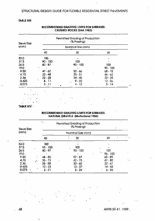
STRUCTURAL DESIGN GUIDE FOR FLEXIBLE RESIDENTIAL STREET PAVEMENTS
TABLE XIII
Sieve Size (min)
53.0 37.5 26.5 19.0 9.50 4.75 2.36 0.425 0.075
TABLE xiv .
Sieve Size (mm)
53.0 37.5 26.5 19.0 9.50 4.75 2.36 0.425 0.075 ,
48
"
RECOMMENDED GRADING LIMITS FOR SUBBASES: CRUSHED ROCKS (SAA 1983)
Permitted Grading of Production (% Passing)
Nnmlnnl Si7p. (mm)
40 30 LU
100 90- 100 100 80 - 87 90- 100 100
90-100 47 - 62 52 -66 68 - 78 32 -48 35-51 46 - 62 22 - 38 24 -40 32 - 38 8 - 1'1 9 - 22 12 - 26 3-;11 11- 12 5- 14
RECOMMENDED GRADING LIMITS FOR SUBBASES: NATURAL GRAVELS (Mulholland 1986)
Permitted Grading of Production (% Passing)
Nominal Size (mm)
. 40 30 ?n
100 95-100 100 80- 97 93 - 100 100
96-100 48 - 85 57 - 87 65-89 35- 73 42 - 75 . 47 -80 25-58 30-60 32 - 67 10-33 13 - 37' 14-42 3- 21 5- 24 . 6- 26
ARRBSR4l.1989.

6. PAVEMENT SURFACING
6.1 GENERAL
The surfacing is an important part of the residential street pavement.ln addition to its technical function. which is discussed in more detail below. the appearance of the surfacing is the means by which users and taxpayers judge the quality of the entire pavement. It is important. ther~fore. that a residential street surfacing should remain free from obvious imperfections and not require frequent maintenance. The user and adjacent residents also require it to have a pleasing appearance. provide good riding quality. be suitable for pedestrian use and produce a low tyre/road noise level.
The technical requirements for the surfacing are that It should:
(a) be impermeable to air and moisture.
(b) have a long service life and be maintenance free for a considerable period.
(c) be flexible and need not have the high resistance to rutting required of more heavily-trafficked pavements.
(d) be of acceptably low level of longitudinal roughn~ss. and
(e) have adequote low speed skid resistance but not necessarily the high surface macrotexture which is required by high speed traffic.
Two surfacing types commonly satisfy these requirements - the spray and chip seal and the thin asphalt surfacing. Under normal circumstances. the designer must decide between these for the residential street pavement. Some of the broad factors that may affect his choice are as follows.
ARRB SR 41. 1989 . 49

STRUCTURAL DESIGN GUIDE FOR FLEXIBLE RESIDENTIAL STREET PAVEMENTS
SPRAY AND CHIP SEALS
Advantages
• Low cost (approx. 1/3 that of 25 mm asphalt) (NAASRA 1985) • Good skid resistance and light reflectance. even in the wet • Reasonable seNice life (7 to 12 years) (NAASRA 1985).
Dlsadvantgges
• Stone loss likely at areas of high traffic stress (e.g. stop lines) • Rough surface for pedestrlon and bicycle troffic • Tracking of precoat or bitumen on tyres onto driveways. etc. • Loose stones from the construction process can be a problem.
ASPHALt
Advantages
• • • Long seNice life (12 to 20 years) (NAASRA 1985) No stone loss likely Pleasant appearance.
Disadvantages
• . For overlays. Increased height can be a problem with gutters and under bridges
• Hlghe,r cost than spray and chip seal.
Thin asphalt surfaclngs. ratherthan spray ond chip s8nls.ore mo~t common In residential streets in the large urban centres. This may be due more to the desire of residents to have an aesthetically pleasing street surfacing which adds t6 the value of their property. rather than to technical considerations.
Further details relating to the spray and chip seal and the thin asphalt surfacing are given In the Sections which follow.
6.2 SPRAYED SEALS
6.2.1 Design References and Procedures
Full Information on the selection of materials and on the design and construction of sprayed seals Is given In the NAASRA publication: Bltumlnuous Surfacing Vol. 1 - Sprayed Work (NAASRA 1984a) The
50 ARRB SR 41. 1989
STRUCTURAL DESIGN GUIDE FOR FLEXIBLE RESIDENTIAL STREET PAVEMENTS
information given below is intended to supplement this and to draw attention to important areas. Dickinson (1984) further assists the designer's understanding of the subject.
The design procedure used in Australia is based on the method first developed in New Zealand ( Hanson 1935).lt depends on the assumption that. after rolling and particle orientation by traffic. the aggregate particles in a seal will lie close packed as a single layer with their least dimension vertical. The average thickness of this layer is the average least dimension of the stones (ALD).lhe design intention Is to fill a predetermined proportion of the voids in this layer with bitumen.
The essential features of the design method are as follows.
(1) The average least dimension (ALD) of the sealing aggregate is determined using a simple sieving procedure.
(2) The percentage of the theoretical surface voids to be filled by bitumen depends on the degree of traffic compaction the surfacing will receive. This percentage is obtained from a table (NAASRA 1984a). For the normal residential street situation. a value of 90 or 95 per cent should be used.
(3) The bitumen application rate. expressed in L/m2• is then calculated from a simple expression involving the ALD and per cent voids filled.
(4) Adjustments to the application rate are then made to allow for the texture and absorptivity of the surface to be treated.
(5) For traffic flows of less than SOOveh/d. a fluxing oil. normally diesel. may be added to the bitumen to soften it and help to ensure that the seal is adequately compacted by the low level of traffic.
(6) The aggregrate application rate is calculated from the ALD with an allowance being made for imperfect spreading and initial losses due to traffic action.
The calculated application rates may be modified further. depending on local experience with the materials used.
There may be situations where a two-coat seal should be considered - despite the added cost involved.Two-coat seals provide longer life. smoother surface texture. (similar to that of an asphalt) and less loss of aggregate in areas where traffic stresses are high such as at stop lines. While guidance on the design of such seals can be given (NAASRA 1984a). some experience is always necessary to judge the correct application rates.
ARRB SR 41. 1989 51
STRUCTURAL DESIGN GUIDE FOR FLEXIBLE RESIDENTIAL STREET PAVEMENTS
6.2.2 Material Specification
To achieve a good result inthe field, the designer must carefully specify the right type of aggregate and the right class of bitumen. Guidelines are provided below.
Aggregate
Crushed rock is normally used for sealing aggregate but in some areas natural gravel may be the only material available. In this case, it is normal to specify that at least 75 per cent by mass should have two or more faces produced by crushing.
It is Important that the aggregate should be relatively single sized and fairly cubical In shape.Simple tests are used to measure and control particle shape and grading (NAASRA 19840). The aggregate must be able to resist decomposition on exposure and must have sufficjent strength and resistance to wear for the expected traffic conditions.For-~ areas where high values of skid resistance must be maintained or where the aggregate will be subject to severe traffic polishing, a material with a high Polished Aggregate Friction Value should be used (SAA 19840 and b). Information on the range of aggregate tests used Is given by Dickinson (1984).
Sealing aggregate is normally precoated with diesel fuel, tar, bitumen or an oil-based proprietary agent. The main purpose of this is to wet any dust on the surface of the aggregate and to allow adhesion of the bitumen binder to the surface of the aggregate after spraying. The rate of application of precoat depends on the size, cleanliness, type and dampness of the aggregate being used. For diesel fuel the rate is normally In the range 6 to 12 L/m2.Adhesion agents should be added if there is a possibility of rain during or shortly after construction.These agents are preferably added to the precoat but may be added to the bitumen shortly before spraying.
Bitumen
Class 170 bitumen is normally used for sealing and the required properties are given In AS 2008 (SAA 19800). If the aggregate used in a sprayed surfacing Is durable and the base remains structurally sound, then the life of the surfacing may be determined by the durability of the bitumen. Bitumen hardens by oxidation until it reaches a level where it cracks or falls to hold the surface stones and surfaCing distress occurs.
The resistance of a bitumen to oxidation hardening is measured by the ARRB Durability Test (SAA 1980b). Road trials have shown the relation-
52 ARRB SR 41, I YIW

STRUCTURAL DESIGN GUIDE FOR FLEXIBLE RESIDENTIAL STREET PAVEMENTS
ship which exists between the Durability Test result and hardening on the road (Oliver 1984). A minimum durability value of nine days is commonly required for Class 170 bitumen and should be specified to ensure adequate seal life.
6.2.3 The Construction Process
To place a durable seal with a satisfactory surface requires care, experience and skill on the part of the laying crew and the supervising personnel. Most problems with seal performance can be traced back to lack of care or attention to detail during the construction process.
It is not possible to describe the process in detail here and the reader is referred to the appropriate publications (NAASRA 19840; Dickinson 1984).
Some important pOints are as follows.
•
•
•
•
•
•
•
For an initial seal the preparation of the surface which is to receive the seal is most important. Any irregularities will reflect through the seal and subsequent reseals.
When an initial seal (not a primerseal) is being placed, the surface should be primed and sufficient time left for the prime to cure.
Bitumen sprayers should be regularly calibrated. The jets should be undamaged and properly aligned and frequent checks for blocked jets should be made. .
The correct bitumen application rate, cutter content and spraying temperature should be used. If the sprayer calibration I~ suspect, this can be checked relatively easily in the field using the carpet tile method (Tredrea 1985).
The correct aggregate application rate should be used. Insufficient coverage results in 'fatty' areas. Over-application restricts optimum stone orientation, results in wastage and creates a potential traffic hazard.
Field measurements need to be taken at the completion of each sprayer run to ensure that the specified bitumen and aggregate application rates are within acceptable tolerances. Standard daily record sheets are readily available for this purpose.
Traffic speeds should be kept low forthe first hour or so after laying, possibly by leading traffic through behind a roller. The Important particle orientation process is started by rolling but is completed by the action of low speed vehicle tyres. If high speed traffic
ARRB SR 41, 1989 53

STRUCTURAL DESIGN GUIDE FOR FLEXIBLE RESIDENTIAL STREET PAVEMENTS
travels over the surface before a reasonable degree of particle interlock has occurred, then the seal may be permanently damaged through stone loss.
6.3 ASPHALT
6.3.1 Design References and Procedures
The primary reference on the subject of asphalt mix design is the NAASRA publication: Biturninuous Surfacing. Vol. 2'- Asphalt Work (NAASRA 1984b). Personnel conce~ned with the specification and placement of asphalt surfaclngs should also use the Asphalt (Hot Mix) Paving - Guide to Good Practice, AS 2734 (SA A 1984a) when preparing the actual construction specification. Further background information on the subject is given in Dickinson (1984).
Two procedures are used to design asphalt mixes in Australia. The most commonly used Is the Marshall method.ln New South Wales, however. the modified Hubbard Field method is often preferred. Both procedures are described in detail in NAASRA (1984b). In order to design a mix using either method, it is necessary to have access to a properly equipped laboratory 'staffed by experienced personnel. For this reason, few Local Government Authorities have designed their own residential street mix, and the more common practice has been to specify State Road Authority (SRA) - designed mixes because these mixes are readily available and are able to be specified by adopting the SRA standard specification.
A note of caution is given here that these mixes do not always perform under light traffic conditions. ARRB research (Oliver 1979) has shown that highway-type mixes, particularly when laid as a thin layer, can have a high air void content immediately after placement and heavy traffic is necessary to produce post-construction densification.When such mixes are laid on residential streets the traffic is usually not heavy enough to compact them further and a high air void content remains.The result is that there is an increased access of air to the interior of the mix and therefore a greater possibility of the bitumen hardening prematurely. Oliver suggests that there may be a substantial benefit in terms of service life achieved by a more critical look at mix design and mix selection for residential streets and it is. suggested (Oliver 1986) that there may be the potential to double service life.
6.3.2 Mix Design
In highway-type mixes, experience over decades has established, with a fair degree of confidence, the relationship between laboratory compaction and field compaction (I.e. the compaction at construction plus the further compaction under traffic).This is not the case in residential mix design. Here, experience is presently lacking to enable
54 ARRB'SR 41, 1989

STRUCTURAL DESIGN GUIDE FOR FLEXIBLE RESIDENTIAL STREET PAVEMENTS
the determination of the correct number of blows in the laboratory to replicate field compaction. In residential streets. the degree of compaction at construction is maintained over life. with little if any further compaction by traffic.
As well as asphalt mixes. there are other mixes which have often been found to be very satisfactory in service in overseas environments.Many contain more bitumen and sand than asphalt and may lead to rutting in hot environments. Examples include: hot rolled asphalt. gap-graded mixes and stone filled sheet asphalts. There is no approved Australian design method for these mixes and yet they may provide adequate service.Therefore. they must be assessed in particular localities and their performance observed underthe relevant conditions of climate. traffic. etc. and their performance compared with more conventional AI.IMralinn mixes.
Two types of mix recommended here are as follows:
ARRB Gap-graded Mix
ARRB developed a gap-graded design because such mixes are easy to compact. so a low air void content is obtained at construction and no traffic compaction is necessary (Oliver 1986).ln addition less of the voids in a gap-graded mix are interconnected than in a continuously graded mix with the same air void contents and this, helps reduce the rate of bitumen hardening. It is possible to manufacture a similar mix by approximately matching the aggregate composition and bitumen content given in Table XV. Since the properties of the fine aggregate are very important in this type of mix. the proportion of (angular) crushed rock fines to (rounded) sand is given. rather than a combined aggregate grading. Approximately 7 per cent of the combined aggregate should pass the 0.075 mm sieve so the amount of added filler will need to be adjusted depending on the proportion of material. in the sand and crusher dust fractions. which posses the 0.Q75 mm sieve.
The bitumen content can be varied by a small amount depending on experience with the laid material.Some experimentation may be nec" essary to determine the best compaction procedure as gap-graded mixes are more prone than dense-graded mixes to shove in front of the roller and produce cracks if rolled at too high a temperature. The compacted mix has a smooth and dense surface texture with a sandy appearance.
High Bitumen Content Mixes
The Road Construction Authority of Victoria (RCA) has designed a series of mixes by modifying the conventional highway mix to be more suitable for lightly-trafficked streets. The main change has been
ARRO SR 41. 1989 55
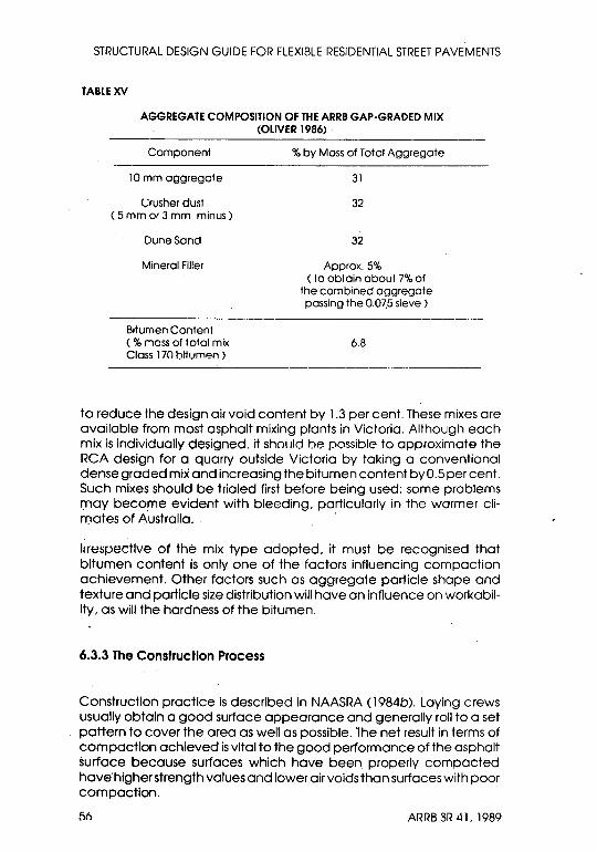
STRUCTURAL DESIGN GUIDE FOR FLEXIBLE RESIDENTIAL STREET PAVEMENTS
TABLE XV
AGGREGATE COMPOSITION OF THE ARRB GAP-GRADED MIX (OLIVER 1986)
Component
10 mm aggregate
Crusher dust ( 5 mm or 3 mm minus)
Dune Sand
Mineral Filler
Bitumen Content ( % moss of total mix Closs 170 blt'.lmen )
% by Moss of Total Aggregate
31
32
32
Approx.5% ( to obtain about 7% of
the combined aggregate passing the 0.07.5 sieve)
6.8
to reduce the design air void content by 1.3 per cent. These mixes are available from most asphalt mixing plants in Victoria. Although each mix is individually designed. it shol lid be possible to approximate the RCA design for a quarry outside Victoria by taking a conventional dense graded mix and increasing the bitumen content byO.5 per cent. Such mixes should be trialed first befare being used; some problems may beco.me evident with bleeding. particularly in the warmer cli-mates of Australia. . .
irrespective of the mix type adopted. it must be recognised that bitumen content is only one of the factars influencing compaction achievement. Other factars such as aggregate particle shape and texture and particle size distribution will have an influence on workabilIty. as will the hardness of the bitumen.
6.3.3 The Construction Process
Construction practice Is described in NAASRA (1984b). Laying crews usually obtain a good surface appearance and generally roll to a set pattern to cover the area as well as possible. The net result in terms of compaction achieved is vital to the good perfarmance of the asphalt surface because surfaces which have been properly compacted have' higher strength values and lower air voids than surfaces with poor compaction.
56 ARRB 3R 41. 1989
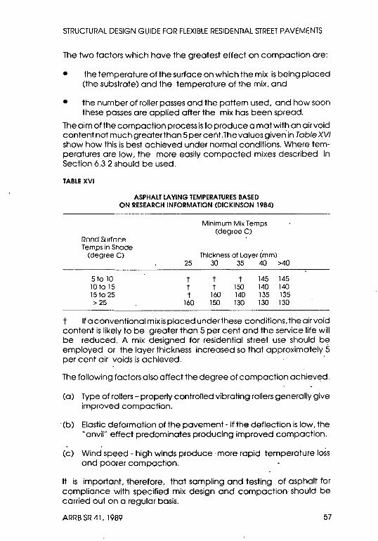
STRUCTURAL DESIGN GUIDE FOR FLEXIBLE RESIDENTIAL STREET PAVEMENTS
The two factors which have the greatest effect on compaction are:
• the temperature of the surface on which the mix is being placed (the substrate) and the temperature of the mix, and
• the number of roller passes and the pattern used, and how soon these passes are applied after the mix has been spread.
The aim of the compaction process is to produce a mat with an airvoid content not much greater than 5 per cent .The values given' in Table XVI show how this is best achieved under normal conditions. Where temperatures are low, the more easily compacted mixes described In Section 6.3.2 should be used.
TABLE XVI
ASPHALT LAYING TEMPERATURES BASED ON RESEARCH INFORMATION (DICKINSON 1984)
Rnnd SlIJfnr.p. Temps in Shade
(degree C)
5to 10 10to 15 15 to 25 > 25
Minimum Mix Temps (degree C)
Thickness of Loyer (mm) 25 30 35 40 >40
t t t
160
t t 145 145 t 150 140 140
160 140 135 135 150 130 130 130
t If a conventional mix is placed underthese conditions, the air void content is likely to be greater than 5 per cent and the service life will be reduced. A mix designed for residential street use should be employed or the layer thickness increased so that approximately 5 per cent air voids is achieved.
The following factors also affect the degree of compaction achieved.
(a) Type of rollers - properly controlled vibrating rollers generally give improved compaction.
(b) Elastic deformation of the pavement - if the deflection is low, the "anvil" effect predominates producing improved compaction.
(c) Wind speed - high winds produce· more rapid temperature loss and poorer compaction.
It is important, therefore, that sampling and testing of asphalt for compliance with specified mix design and compaction should be carried out on a regular basis.
ARRB SR 41. 1989 57

7.CONSTRUCTION STANDARDS
7.1 GENERAL
The quality af construction. to 0 very large extent. will determine the performance of a flexible' pavement structure. This quality must commence from the outset with the preparation of the subgrade and any underlying fill. and continue through to the completion of the laying of the pavement surfacing.
An.essential part of the design process. therefore. is a description of the. construction standards or controls to ensure the realisation of the assumptions made as the basis of the final design. These standards must relate'to general earthworks. subgrade. subbase. basecourse and pavement surfacing. that is . to the total construction process. as outlined In the paragraphs which follow.
7.2 GENERAL EARTHWORKS
As a first step to general earthworks. clearing and grubbing should be -carried out and all top soil removed. Any fill should then be placed In layers to achieve a minimum density of 95 per cent standard compaction (AS 1289 of SAA 1977 a). Proof rolling may be used to ensure that no soft spots occur within the fill. This should be done following on closely from the completion of normal rolling. A fully ballasted self-propelled three wheel steel-wheeled roller. heavy pneumatic tyred roller with high contact pressure or loaded truck should be used for this exercise.
7.3 SUBGRADE PREPARATION
T(1e top 150 mm of the subgrade formation should be compacted to 100 per cent standard compaction.
Care must be taken to ensure that no discontinuities exist across the width of the subgrade. A typical example would be an existing unsealed road of narrow width with table drains. which is to be widened -and reconstructed to urban-type standards. with its
58 ARRB SR 111. 1989
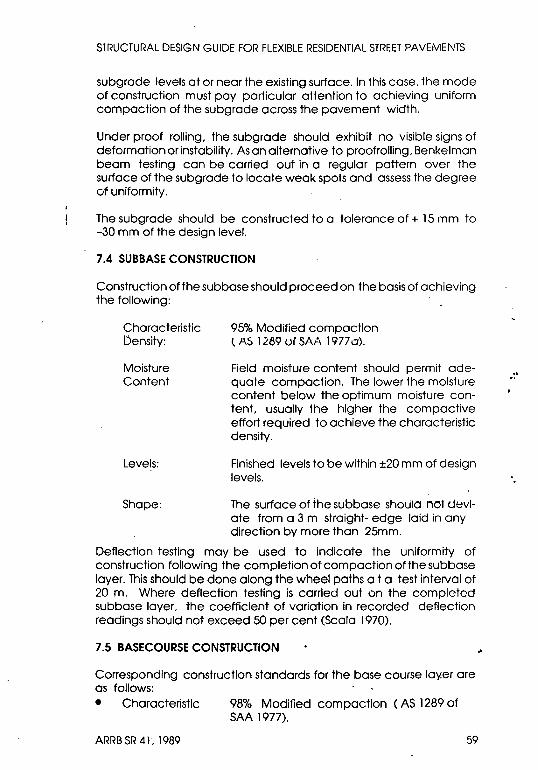
STRUCTURAL DESIGN GUIDE FOR FLEXIBLE RESIDENTIAL STREET PAVEMENTS
subgrade levels at or near the existing surface. In this case. the mode of construction must pay particular attention to achieving uniform
. compaction of the subgrade across the pavement width.
Under proof rolling. the subgrade should exhibit no visible signs of deformation or instability. As an alternative to proofrolling. Benkelman beam testing can be carried out in a regular pattern over the surface of the subgrade to locate weak spots and assess the degree of uniformity.
The subgrade should be constructed to a tolerance of + 15 mm to -30 mm of the design level.
7.4 SUBBASE CONSTRUCTION
Construction of the subbase should proceed on the basis of achieving the following:
Charocteristic Density:
Moisture Content
Levels:
Shape:
95% Modified compaction t AS 1289 ur SAA 19770).
Field moisture content should permit adequate compaction. The lower the moisture content below the optimum moisture content. usually the higher the compactive effort required to achieve the characteristic density.
Finished levels to be within ±20 mm of design levels.
The surface of the subbase shOljlO nol deviate from a 3 m straight- edge laid in any direction by more than 25mm.
Deflection testing may be used to indicate the uniformity of construction following the completion of compaction of the subbase layer. This should be done along the wheel paths a t a test interval of 20 m. Where deflection testing is carried out on the completed subbase layer. the coefficient of variation In recorded deflection readings should not exceed 50 per ceht (Scala 1970).
7.5 BASECOURSE CONSTRUCTION
Corresponding construction standards far the base course lay.er are as follows: • Characteristic 98% Modified compaction (AS 1289 of
SAA 1977).
ARRB SR 41. 1989 59
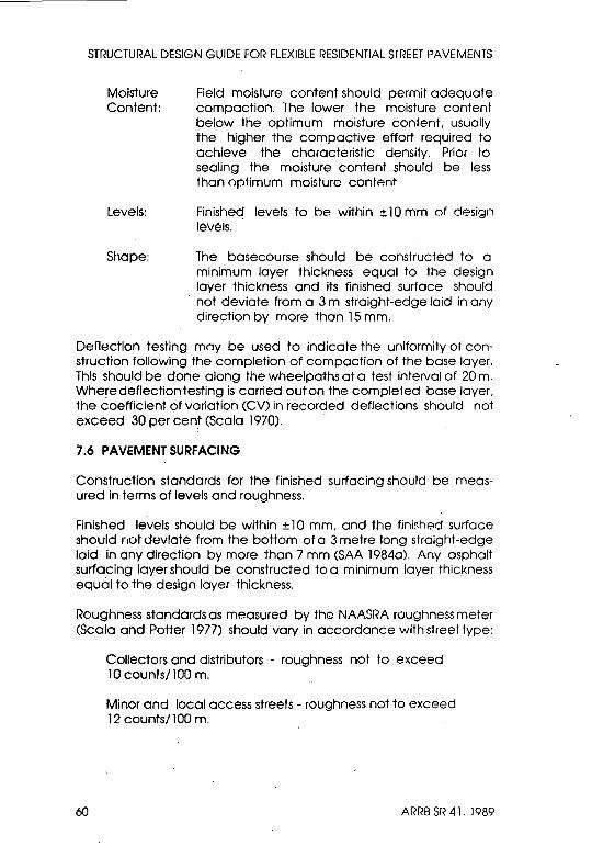
STRUCTURAL DESIGN GUIDE FOR FLEXIBLE RESIDENTIAL STREET PAVEMENTS
Moisture Content:
Levels:
Shape:
Field moisture content should permit adequate compaction. The lower the moisture content below the optimum moisture content. usually the higher the compactive effort required to achieve the characteristic density. Prior to sealing the moisture content should be less than optimum moisture contp.nt
Finished levels to be within ~ 10 mm of design levels.
The basecourse should be constructed to a minimum layer thickness equal to the design layer thickness and its finished surface should
. not deviate from a 3 m straight-edge laid in any direction by more than 15 mm.
Denectlon testing may be used to indicate the uniformity of construction following the completion of compaction of the base layer. This should be done along the wheelpaths at a test interval of 20 m. Where deflection testing is carried outon the completed base layer. the coefficient of variation (CV) in recorded deflections should not exceed 30 per cenJ' (Scala 1970). .
7.6 PAVEMENT SURFACING
Construction standards for the finished surfacing should be measured in terms of levels and roughness.
Finished levels should be within ± 1 0 mm. and the finished surface 3hould noldevlate from the bottom ofa 3 metre long straight-edge laid in any direction by more than 7 mm (SAA 1984a). Any asphalt surfacing layer should be constructed to a minimum layer thic,kness equOi to the design layer thickness.
Roughness standards as measured by the NAASRA roughness meter (Scala and Potter 1977) should vary in accordance with street type:
60
Collectors and distributors - roughness not to exceed 10 counts/ 100 m.
Minor and local access streets - roughness not to exceed 12 counts/l00 m.
ARRB SR 41. 1989

REFERENCES
AMERICAN .A'3"nC:IATION OF STATE HIGHWAY AND TRANSPORTATION OFFICIALS (1985). Proposed AASHTO guide for design of pavement structures. Volumes 1 and ? NCHRP project 20-7/24.
AUFF, AA (1983). Quality control of dimensions In road construc-tion. Australian Road Research Board. Special Report SRNo. 2~. .
__ (1986). The selection of statistical control schemes forconstruction quality control. Australian Road Research Board. Special Report SRNo. 30. .
AUSTRALIAN ASPHALT PAVEMENT ASSOCIATION (1983). Structural design of flexible pavements. Manual No.1. AAPA,Melbourne.
BARNARD, P. (1986). Data collection and statistical analysis tecniques for deriving pavement design curves. Australian Road Research Board. Internal Report, AIR 392-5.
BARRY, I.M. (1986). The influence of trees and. shrubs on pavement 1055 of shape. Road Construction Authority of Victoria. Technical I~eport 75. RCA. Melbourne.
CEMENT AND CONCRETE ASSOCIATION OF AUSTRALlA(1984a). Concrete street and parking area pavement design. T33. CACA, Sydney.
__ (1984b). Single lane bus bays. TN52. CACA, Sydney.
__ (19860). Interlocking pavements - a guide to design and construction. TN35. CACA, Sydney.
__ (1986b). Guide specification for construction of Interlocking concrete road pavements. TN56. CACA. Sydney.
ARRB SR 41. 1989 61

STRUCTURAL DESIGN GUIDE FOR FLEXIBLE RESIDENTIAL STREET PAVEMENTS
CONCRETE MASONRY ASSOCIATION OF AUSTRALIA (1986). Specification for concrete segmented paving units. MA 20. CMAA. Sydney.
DEPARTMENT OF MAIN ROADS. NEW SOUTH WALES (1983). Pavement thickness design. M.R. Form No. 76. DMR. Sydney.
DICKINSON. E.J. (1984). Bituminol IS Roads in Australia. Australian Road Research Board.
DI\I.W. P.J. (1981). f'lexlble road pavement thickness design for residential streets. Final year Project Report to Dept Civil Engi neering. Unlv. of Newcastle. NSW.
DUNLOP, R.J. ( 1980). A review of the design and performance of roads incorporating lime and cement stabilised pavement layers. Australian Road Researdh Board ARRJournal. Sept. 1980. Vol 10. NO.3
FEDERAL HIGHWAY ADMINISTRATION (1979). Technical guide lines for expansive soils in highway subgrades. Report No. FHWA-RD-79-51. FHWA. Washington. D.C.
GERKE. R.J. (1987). Subsurface drainage of road structures. Australian Road Research Board. Special Report SRNo. 35.
HANSON. F.M. (1935). Bituminous surface treatment of rural highways. Proc. New Zealand Soc. Clv. Eng. 21 (1934-35). pp. 247-59.
INDIAN ROADS CONGRESS (1984). Guidelines for the design of flexible pavements. IRC, New Delhi.
JONES. EA and MALLON. P. (1983). Pavement analysis and design by Benkelman Beam. Proc. 2nd Nat. Conf. on Local Government Eng .. PP. 325-29. Brisbane.
KNAPTON, J. and MAVIN. K.C. (1987). Clay segmental pavements. Brick Development Research Institute/Australian Clay Brick /\sso· clatlon/Royal Melbourne Institute ofTechnology.
LAY. M.G. and METCALF. J.B. (1983). Soil stabilisation in Australia. Proc. 2nd Nat. Conf. on Local Government Eng. pp. 346-51. Brisbane.
__ (1985). Source Book for Australian Roods: Third Edition. Australian Road Research Board.
_. _ (1986). Handbook of Rood Technology. Gordon and Breach: London
02 ARRB SR 41. 1989

STRUCTURAL DESIGN GUIDE FOR FLEXIBLE RESIDENTIAL STREET PAVEMENTS
MAIN ROADS DEPARTMENT, QUEENSLAND (1981). Interim manual for the design of flexible pavements.
METCALF, J.B. (1977). Principles and application of cement and lime stabilisation. Australian Road Research Board, Research Report ARR No. 49.
MciNNES, D.B. (1986). Drying effect of different verge planted tree species on urbon roods. Proc. 13th ARRB Conf. 13(4), pp. 54-66.
MULHOLLAND, P. J., (1988), Pavement design variable and street construction cost, Proc. NSW LGEA Conf., Sydney
__ SCHOFIELD, G.M. and ARMSTRONG, P. (1986). Structural design criteria for residential street pavements: interim rep,ort based on Stage 1 of ARRB Project 392. Australian Road Research Board. Research Report, ARR Nu. 140.
__ (1987) Structural design guide for residential street pavements: preliminary draft. Australian Road Research Board. Research Report ARR No. 150
NATIONAL ASSOCIATION OF AUSTRALIAN STATE ROAD AUTHORITIES: (1974). A guide to the selection and testing of gravel for pavement construCtion. NAASRA, Sydney.
__ (1979). Interim guide to pavement thickness design. NAASRA, Sydney.
__ (1984a). Bituminous surfacing. Vol. 1 - Sprayed Work. NAASRA, Sydney.
__ (1984b). Bituminous surfacing. Vol. 2 - Asphalt Work. NAASR,A., Sydney.
_._ (1985). Guide to the selection of bitGminous surfacing for
pavements. NAASRA, Sydney.
__ (1986).Guide to stabilisation in roadworks. NAASRA, Sydney.
__ (1987). Pavement design: A guide to the structural design of road pavements. NAASRA, Sydney.
OLIVER, J.w.H. (1979). Asphalt mixes for residential streets. Fourth Int. Conf. of Aust. Asphalt Pavement Assoc., Melbourne.
ARRB SR 41, 1989 63

STRUCTURAL DESIGN GUIDE FOR FLEXIBLE RESIDENTIAL STREET PAVEMENTS
_'_(1983). Road trials laid to evaluate mix designs for resurfacing lightly trafficked residential streets. Australian Road Research Board. Research Report. ARR No. 125.
__ (1984). An Interim model for prediCting bitumen hardenIng in Australian sprayed seals. Proc. 12th ARRB Conf. 12(2). pp. 112-20.
__ ' (1986). Road trials to evaluate mix designs for resurfacing residential streets: results after 6 years. Australian Road Research Board. Internal Report AIR 305-2.
PITMAN. C.J .. IASIELLO. W.N .. MciNNES. D.B. (1985). Investigations into residential street pavements on expansive clay subgrades. Proc. 3rd National Conf. on Local Government Eng .. pp. 130--33. Melbourne.
SCALA. A.J. (1970). The use of Benkelman beam deflection test in control of construction and work. Proc. 5th ARRB Conf.. 5(5). pp. 181-94.
__ and POTIER. D.W. (1977). Measurement of road roughness. Australian Road Research Board. Technical Manual ATMNo. 1.
SCHOFIELD. G.M. (1985). Traffic as a design variable for residential str~~t pavements. Australian Road Research Board. Internal Report. AIR 392-4.
__ . MULHOLLAND. P.J. and MORRIS. P.O. (1984). State of the ort report. Design and maintenance of residential street pavements. Australian Road Reseorch Board. Internal Report. AIR 392-1.
STANDARDS ASSOCIATION OF AUSTRALIA (19770). Methods of testing soils for engineering purposes. AS 1289. SAA. Sydney.
__ (l977b). Draft Austra lion Standard for aggregate and rock for engineering purposes. Part 3 -pavement base and subbase. DR 83181. SAA. Sydney.
__ (19800). Residual bitumen for pavements. AS 2008. SAASydney.
__ (1980b). Methods of testing bitumen and related road making products. AS2341 Section 13. Durability of bitumen. SAA. Sydney.
__ (1981). The site Investigation code. AS 1726. SAA. Sydney.
__ (1984a) . .Asphalt (hot-mixed) paving - guide to good practice. AS 2734. SAA, Sydney.
ARr~B sr~ 41.IY/lY

STRUCTURAL DESIGN GUIDE FOR FLEXIBLE RESIDENTIAL STR~ET PAVEMENTS
__ (1984b). Laboratory polishing of. aggregate using the verti-cal road wheel machine. ASl141.40. SAA. Sydney. . - . __ (l984c). Laboratory polishing of· aggregate using the hori-
zontal bed machine. AS 1141.41. SAA. Sydney. -
__ (1986). Road and traffic engineering - glossary of terms . .Part 1 - Road design and construction. AS 1348.1. SAA. Sydney.-
TREDREA. P.F. (1985). Measurement ofthe application rates of scrap rubber modified bituminous binders. Australian Road Research Board. Internal Report. AIR 286-12.
ARRB SR 41. 1989 65

APPENDIX A PAVEMENT THICKNESS DESIGN: WORKED EXAMPLES
A.1 DESIGN FOR URBAN CONSTRUCTION
Three worked examples are given:
it Worked Example No. 1 considers design of a new pavement in ci cul-de-sac where design traffic is less than 105 ESA (Section A.l.l).
• Worked Example No.2 illustrates the further check that should be mode to prevent fatigue crocking occurring in an asphalt surfacing layer which is more than 25 rl)m thick. in the particular Instance where the design traffic value exceeds 105 ESA (Section A.1.2). .
• Worked Example No.3 illustrates design of an existing local access pavement which is to undergo total reconstruction (Section A. 1 :3).
A. 1.1 Worked Example No.1:
A new pavement of urban-type construction where the design traffic value Is :::;;105 ESA. Design curves are based on the confidence limit of 90 per cent
DATA: Street Description
Subgrade
Cul-de-sac of 100 m length
Heavy cloy (CH) along entire length with Laboratory soaked CBRs recorded of 3.0, 4.5 and 4.0; PI = 25.
Dynamic cone results from. three year old pavements located nearby gave In situ.CBRs on the some heavy clay of 5.4,7.8 and 15.
66 ARRB SR 41. 1989

STRUCTURAL DESIGN GUIDE FOR FLEXIBLE RESIDENTIAL STREET PAVEMENTS
800mm Rainfall Drainage Good site with subsoil drains to be pro
vided Traffic Design Life (P)
DESIGN CALCULATIONS
Anticipated AADT 150 30 years
(i) Design CBR Least of Lob. CBRs x Fodor from Table IV for PI > 11 3.0x 1.4 4.2. say. 4.0
Importantly. thic value is confirmArl hy thA results ogtained from .the pavements nearby.
(ii) Design Traffic
AADT N, Y Ng
Design Traffic
Construction ESAs + In-service ESAs + Garbage ESAs
= .1 AAm + N,.365,Y + Ns .52.P
150 (from given data) 0.4 (from Tobie VII) P = 30 (Section 3.2.2) 2.60 x 1 x 0.5 = 1.3 (Section 3.2.4)
3 x 150 + 0.4 x 365 x 30 + 1.3 x 52 x 30 450 + 4380 + 2028 6860. say. 6.9 x ]()I ESA
Note that this value is within the range given for Minor Streets In Tobie VIII.
(iii) Design Thickness from Fig. 10 = 265 mm
(iv) Pavement to be composed of. say:
i:~~~;~~~:;ng E . ~~t~:~~,~ Fora design traffic of6.9x 1()3 ESA and a design CBR of 30 (see Fig. 7(}). the required depth of cover over subbase is 100 mm which is satisfied by the above.
A.l.2 Worked Example No.2:
A new pavement. of fixed level construction where· the design traffic value> 105 ESA. Design curves are based on the confidence limit of 95 per cent.
ARRB SR 41. 1989 67

STRUCTURAL DESIGN GUIDE FOR FLEXIBLE RESIDENTIAL STREET PAVEMENTS
DATA:
Street Description
Subgrade
1st 500 rn
2nd 1000 m
Rainfall
Drainage
Traffic
No. of light buses per day, per lane
No. uf garbage trucks'per week
Design Life (P)
Collector of 1500 m length.
Silty clay (CL) with Lab. soaked CBRs recorded uf 5,7,6,8 and 4.h: PI = 17.
Clayey sand (SC) with Lob. soaked CBRs recorded of 14. 18, 12.9 and 12; PI ==10.
1200 mm
Fair with subsoil drains to be provided
500veh/d at year 0 2500 veh/d at year 5 then increasing by 2% per annum
10
5
30 years
N.B. Traffic capacity assumed not to be exceeded in the 30 years.
DESIGN CALCULATIONS:
(i) Design CBR for 1st 500 m
Design CBR for 2nd 1000 m
.6R
10th percentile of 5 Lab. CBRs x 0.8 (Factor from Table IV for PI > 11) (6.1 - 1.3 x 1.27) x 0.8 3.6, say, 3.5
10th percentile of 5 Lab. CBRs x 0.65 (Factor from Table IV for PI < 11) (13.0 - 1.3 x 2.97) x 0.65 6.5, say, Z
AI~I~B SR 41. 1989

STRUCTURAL DESIGN GUIDE FOR FLEXIBLE RESIDENTIAL STREET PAVEMENTS
(ii) Design Traffic
AADT N,
P
Y
Nb ~jg
Design Traffic
Construction ESAs + In-service ESAs + Bus ESAs + Garbage ESAs 3.AADT + N,.365.Y + N
b.365.Y + Ng,s2.P
2500 (from given data) 30 (from Table Vlf)
28 years (to take into account initial build-up in traffic)
(1 + 0.02)28 -1
In (1 + 0.02)
0.7410. -- = 37.4 (Section 3.2.2) 0.0198
10 x 1.0 = 10 (Section. 3.2.3) 0;0 ~,60 )( fi)( 1,0 "" 13 (Section 3.2.4)
3 x 2500 + 30 x 365 x 37.4 + 10 x 365x 37.4 + 13 x 52 x 28 7500 + 409 530 + 136510 + 18928. 572 468, say, 5.7 x 10⁵ ESA
Note that this value is just within the range given for Collectors in Table VIII.
(iii) Design Thicknesses from Fig. 7:
495mm For 1st 500 m For 2nd 1000 m = 310 mm
(iv) Pavements to be composed of. say:
1st Section Asphalt Surfacing = 30mm
Base Loyer. l00mm
Subbase Layer 365mm
2nd Section Asphalt Surfacing 30mm
Base Loyer l00mm
Subbase Layer 18Qmm
ARRB SR 41, 1989 69
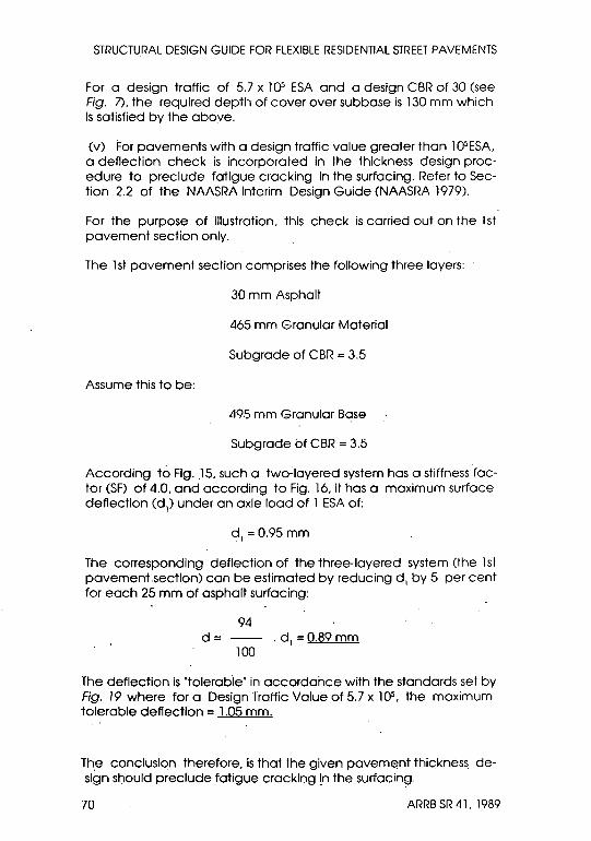
STRUCTU.RAL DESIGN GUIDE FOR FLEXIBLE RESIDENTIAL STREET PAVEMENTS
For a design traffic of 5.7 x 10⁵ ESA and a design CBR of 30 (see Fig. 7), the required depth of cover over subbase is 130 mm which Is satisfied by the above.
(v) For pavements with a design traffic value greater than lOSESA, a deflection check is incorporated in the thickness design procedure to preclude fatigue cracking in the surfacing. Refer to Section 2.2 of the NAASRA Interim Design Guide (NAASRA 1979).
For the purpose of illustration, this check is carried out on the 1st pavement section only.
The 1st pavement section comprises the following three layers:
30 mm Asphalt
465 mm Granular Material
Subgrade of CBR = 3.5
Assume this to be:
49.5 mm Granular Base
Subgrade bf CBR = 3.5
According to Fig . .15, such a two~layered system has a stiffnessfactor (SF) of 4.0, and according to Fig. 16, it has a maximum surface deflection (d)) under an axle load of 1 ESA of:
d1 =0.95 mm
The corresponding deflection of the three-layered system (the 1 st pavement.sectlon) can be estimated by reducing d 1 by 5 per cent for each 25 mm of asphalt surfacing:
94 d = -- . d 1 = 0.89 mm
100
The deflection is 'tolerable' in accordance with the standards set by Fig. 79 where for a Design Traffic Value of 5.7 x lOS, the maximum tolerable deflection = 1.05 mm.
The conclusion therefore, is that the given pavement thickness design should preclude fatigue cracking [n the surfacing.
7Q ARRB SR 41. 1989
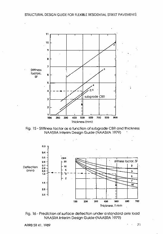
STRUCTURAL DESIGN GUIDE FOR FLEXIBLE RESIDENTIAL STREET PAVEMENTS
Stiffness footon;,
SF
11 ,--,,--,---,---,---,---,---,--,
10
8
7
6
5
4
2
1~~L-~ __ ~ __ -ll __ ~ __ ~ __ -L __ ~
100 200 300 400 500 600 700 800 900
Thickness (mm)
Fig. 15 - Stiffness factor as a function of subgrade CBR and thickness NAASRA Interim Design Guide (NAASRA 1979) .
0.3
0.4
0.5 CBR
0.6
r Deflection 0.7 10 0.8
(mm) 0.9 .-- ~--1.0
1.5
2.0
2.5
100
stifness factor. SF
2
J
5
7
10
200 300 400 500 600 700
Thickness. T mm
Fig. 16 - Prediction of surface deflection under a'standard axle load NAASRA Interim Design Guide-(NAASRA -1979)
ARRB SR 41. 1989 71
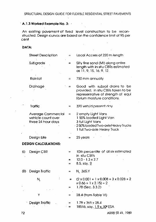
STRUCTURAL DESIGN GUIDE FOR FLEXIBLE RESIDENTIAL STREET PAVEMENTS
. A. 1.3 Worked Example No.3: .
An existing' pavement of fixed level construction to be reconstructed. Design CUNes are based on the confidence limit of 95 per
cent
DATA:
Street Description
Subgrade'
Rainfall
Drainage
Traffic
Average Commercial vehicle count over three 24 hour days
Design Life
DESIGN CALCULATIONS:
(i) Design CBR
(ii) Design Traffic
y
Design Traffic
72
Local Access of 220 m length
Silty fine sand (MI) along entire length with in situ CBRs estimated as 11.9. 15. 16.9. 12.
750 mm annually
Good with subsoil drains to be provided; in situ CBRs taken to be representative of strength at equi librium moisture conditions.
3?O vE'lh/nl'rp.sp.nt noy
2 empty Light Vans 1 50% loaded Light Van 3 full Light Vans
·25O%loadedTwo-axleHeavyTrucks 1 full Two-axle Heavy Truck .
25 years
10th percentile of all six estimated in situ CI3I~s 12.0-1.3x2.7 8.5. say. 2
Nt 365.Y
(2 x 0.001 + 1 x 0.008 + 3 x 0.028 + 2 x 0.66 + 1 x 2.15) + 2 1.78 (Sec. 3.3.2)
28.4 (from Table VI)
1.78 l( .'365 x 28.4 18516, say, l21LJ..Q'I ESA
ARRB SR 41. 1989
~TRUCTURAL DESIGN GUIDE FOR FLEXIBLE RESIDENTIAL STREET PAVEMENTS
Note that In calculating Nt' it was not necessary to apply a factor of 1.5 because the counts covered the full 24 hour day and not 8 hours. Assumed traffic growth factor of 1 per cent was taken from Table VII.
(iii) Design Thickness from Fig. 7 205mm
(Iv) Pavement to be composed of. say:
Asphalt Surfacing
Base Layer
Subbase Layer
100mm
100mm
Note: One cannot use 80 mm layer thickness for a subbase since its specified minimum thickness =·100 mm (see Section ~ 2.1)
For a design traffic of 1.9 x lQ4 ESAs and a design CBR of 30 the required depth of cover over the subbase should be 1.00 mm. which is satisfied by the above.
A.2 DESIGN FOR RURAL CONSTRUCTION
A single worked example is given h'3reunder (Section A.2.1). Because the example assumes a design traffic value of less than 105
ESA. the deflection check for fatigue cracking in the asphalt layer Is not carried out (Section A.l.2).
A.2.1 Worked Example NO.4:
A pavement of rural-type (non-fixed level) construction where the design traffic ~1Q5 ESA. Design curves are based on the confdence limit of 90 per cent.
DATA:
Street Description
Subgrade
Rainfall
Drainage
ARRB SR 41. 1989
. Local Access of 300 m length
Clayey silt (Cl) along' entire length with Lab. CBRs recorded of 10.7.12. 9and7;PI=15. 600mm
. Poor with no subsoil drains provided.
. 73

STRUCTURAL DESIGN GUIDE FOR FLEXIBLE RESIDENTIAL STREET PAVEMENTS
Traffic
Design Life (P)
400 veh/d anticipated AADT; 5% expected commercial vehicle rate, with traffic growth rate of 1 % per annum.
20 years
DESIGN CALCULAtioNs:
(i) Design CBR 10th percentile of 5 Lab. CBRs x 1.4 (Factor from Table IVfor PI > 11) (9.0 - 1.3 x 1.90) x 1.4 9.1. say, 2
(ii) Design Traffic Construction ESAs + In-service ESA's + Gorl;;>oge ESAs
AADT
ESA/CV
N , -
y
Ng
Design Traffic
- 3.AADT + Ns.365.Y + Ng 52.P
400 veh/d (from given data)
0.40 (from Table VI{)
400 5 i -- x -- x 0.04"" 4.0 (!Jec. 3.2.2)
2 100
22.1 (from Table VI)
2.60 x 1 x 0.5 = 1.3 (Para. 3.2.4)
. 3 x 400 + 4.0 x 365 x 22.1 + 1.3 x 52 x 20 1200 + 32412 + 1352 34964, say, ~ ESA
Note that this value is within the range given for Local Access Streets in Table VIII.
(iii) Design Thickness from Fig. 10 = 175 mm
(iv) Pavement to be composed of, say:
Bituminous Seal
Base Layer 175mm
The thin bituminous seal is assumed here not to contribute to the overall strength of the pavement. -
74 , ARRB SR 41. 1989
. STRUCTURAL DESIGN GUIDE FOR FLEXIBLE RESIDENTIAL STREET PAVEMENTS
A.3 DESIGN FOR STAGE CONSTRUCTION
Two worked examples of stage construction are given hereunder.
• Worked Example NO.5 considers design of a cul-de-sac pavement which is to be constructed initially with a bituminous seal below the lip of kerb and channel. then several years later with asphalt flush with the lip of kerb and channel (Sec.A.3.1).
(I Worked Example No. 6 considers design of a local access pavement which is to be constructed initially to non-fixed level (low structural integrity) standards, then a decade later to fixed level standards (Section A.3.2).
A.3.1 Worked Example NO.5:
A fixed level pavement initially constructed with bituminous seal and several years later, covered with asphalt surfacing layer to complete construction. Design curves are based on a confidence
limit of 90 per cent.
DATA:
Street Description
Subgrade
Rainfall
Drainage
Tronic
Cul-de-sac of 80 m length
Heavy clay (CH) along entire length with Lab. soaked CBRs recorded of 2.5 and 3.5; PI = 32.
.1000 mm
Fair site with subsoil drains provided
120 veh/d anticipated AADT 2% comme~cial vehicles
1 st Stage of Construction to achieve a Design Life 3 years
2nd Stage of Construction to achieve a further Design Life 20 years
DESIGN CALCULATIONS:
(i) Design CBR
ARRB SR 41. 1989
Least of Lab. CBRs x Factor from Table IV for PI >11· 2.5 x 1.2 = 3.0 .
75
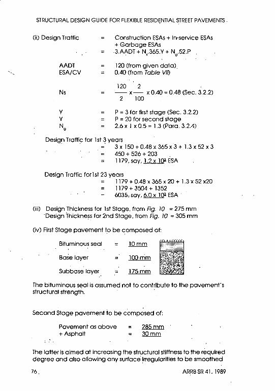
STRUCTURAL DESIGN GUIDE FOR FLEXIBLE RESID~NTIAL STREET PAVEMENTS.
(ii) Design Traffic Construction ESAs + In-service ESAs + Garbage ESAs
AADT ESA/CV
Ns
-. .3.AADT + N .365.Y + N .52.P . , 9
120 (from given data). 0.40 (from Table Vlf)
120 2 - x- x 0.40 = 0.48 (Sec. 3.2.2)
2 100
P = 3 for first stage (Sec. 3.2.2) P = 20 for second stage 2.6 x 1 x 0.5 = 1.3 (Para. 3.2.4)
Design Traffic for 1st 3 years . . . 3 x 150 + 0.48 x 365 x3 + 1.3 x 52 x 3
450 + 526 + 203 . 1 179 , say, l2..xJ.Q3 ESA
Design Traffic forlst 23 years 1179 + 0.48 x 365 x 20 + 1.3 x 52 x20 1179 + 3504 + 1352 6035, 60'1', ~ ESA .
(iii) Design Thickness for 1st Stage, from Fig. 10 = 275 mm 'Design Thickness for 2nd Stage, from Fig. 10 = 305 mm
(iv) First Stage pavement to be ~omposed of:
Bituminous seal
Base layer
Subbase layer
lOmm
100 rrim
175mm
The bituminous seal is assumed not to contribute to the pavement's structural strength. .
Second Stage pavement to be composed of:
Pavement as above + Asphalt
285mm 30mm
The latter is aimed at increasing the structural stiffness to the required degree and also allowing any surface !rregularities to be smoothed
76. ARRB SR 41. 1969

STRUCTURAL DESIGN GUIDE FOR FLEXIBLE RESIDENTIAL STREET PAVEMENTS
out, following the termination of construction traffic. Under such circumstances of light traffic, an additional 30 mm of asphalt should provide the second stage pavement with adequate total design thickness. Deflection testing would be carried out in, say, Year 3 of the First Stage's trafficking to confirm:
(a) the actual timing of the overlay: and (b) the adequacy of a 30 mm overlay.
The overlay design method as outlined in Appendix B would be used for this.
A.3.2 Worked Example NO.6:
A pavement constructed in its firststage.to non-fixed level standards, then in its final stage to fixed level standards. Design curves for the non-fixed level construction are based on a confidence limit of 80 per cent and the curves for fixed level construction are based on the confidence limit of 95 per cent.
DATA:
Street Description
Subgrade
Rainfall
Drainage
Traffic
Local Access of 200 m length
Highly compressible silt (MH) along entire length with Lab. soaked CBRs recorded of 4,3,3 and 4.5: PI = 20.
700 mm annually
Fair site with subsoil drains not provided in the first stage but in the second stage
300 ve,h/d anticipated AADT . 3% commercial vehicles
1 st Stage of Construction to achieve a Design Lif~ 10 years
2nd Stage of Construction to achieve a further Design Life 30 years
DESIGN CALCULATIONS:
(i) Design CBR
ARRB'SR 41. 1989
Least of Lab. CBRs x Factor from Table IV for PI > 11 3.0 x 1.2 3.6,say,~
77
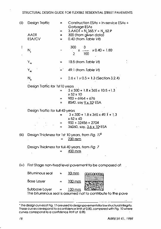
STRUCTURAL DESIGN GUIDE FOR FLEXIBLE RESIDENTIAL STREET PAVEMENTS
(ii) Design Traffic Construction ESAs + In-service ESAs + Garbage ESAs 3.AADT + N 365.V + N .52.P s. g
AADT 300 (from given data) ESA/CV = 0.40 (from Table VI{)
300 ·3 N
5 X x 0.40::: 1.80
2 100
V,O 10.5 (from Table Vf)
Vd[) 49.1 (from Table Vf)
Ng 2.6 x 1 x 0.5 = 1.3 (Section 3.2 . .11)
Design Traffic for 1stlO years 3 x 300 + 1.8 x 365 x 10.5 + 1.3 x 52 x 10 900 + 6964 + 676 8540, say 2..x..l.Q3 ESA
Design Traffic for full 40 years 3 x300 + 1.8 x 365 x 49.1 + '1 .. 3
x 52 x 40 900 + 32456 + 2704 36060, say, 3.6 x 1 ()A ESA
(iii) Design Thickness for 1st 10 years, from Fig. 17-230mm
Design Thickness for full 40 years, from Fig. 7 400mm
(iv) First Stage non-fixed level pavement to be composed of:
Bituminous seal
Base Layer 100mm
Subbase Layer 130 mm The bituminous seal is assumed not to contribute to the pave
• The design curves of Fig. 17 are used to design pavements for low structurallntegrlty. These curves correspond to a confidence limit of 0.80, compared with Fig. 10 where curves correspond to a confidence limit of 0.90.
II:! AI~I~~ Sl~ 41, 191:!9
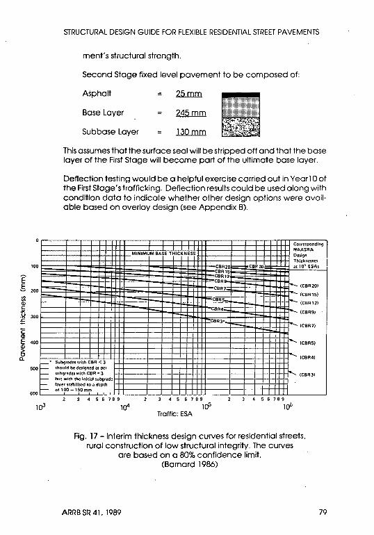
100
E -5 200
~ ()) c ~ 0 300 ~
~ E 400 ())
t5 c.. r-"
500 f--f--'---
600
STRUCTURAL DESIGN GUIDE FOR FLEXIBLE RESIDENTIAL STREET PAVEMENTS
ment's structural strength.
Second Stage fixed level pavement to be composed of:
Asphalt
Base Layer 245mm
Subbase Layer 130mm
This assumes that the surface seal will be stripped off and that the base layer of the First Stage will become part of the ultimate base layer.
Deflection testing would be a helpful exercise carried out in Yearl 0 of the First Stage's trafficking. Deflection results could be used along with condition data to indicate whether other design options were available based on overlay design (see Appendix B).
Co" •• pond;ng I - "!; ..... .... , .. '; .. :!c"!. NAASRA
MINIMUM BASE THICKNfSf Design
::;~~n~~~s I CBR20 I:::::::::::::: C8R30: CBRlS CBR12 CBR9
CBR7 (CBR201
(CBR15! C8R5
(CBR121 - CBR4_ {CBRS!
CBR3" - (CBR71
(CBRS!
(CBR4! Subgrades with CBR < 3 should be designed as per subgrades with CaR c 3 (CBR31 but with the initial subgrade layer stabilised to a depth of 100 - 150 mm
34567B9 3456189 3 456789
,Q'I ,05 1(1' Traffic: ESA
Fig. 17 - Interim thickness design curves for residential streets, rural construction of low structural integrity. The curves
are based on a 80% confidence limit. (Barnard 1986)
ARRB SR 41. 1989 79

APPENDIX B ASPHALT OVERLAY DESIGN
PRELIMINARY NOTES TO THE DESIGN PROCEDURE
Overlays on residential streets are usually asphalt although on.occasions where a thick overlay is called for, an unbound layer may be used or the alternative of cement, lime or bitumen stabilisation' of the basecourse may be adopted. For design using thick overlays of granular materials, the designer is referred to Section 1O.S of the NAASRA Guide to the Structural Design of Road Pavements (1987).
In its Project 392 research, ARRB gathered some test data from which it could outline a procedure for asphalt overlay design. This procedure is based upon deflection analysis, details of which follow In Sections B.l to B.S. .'
However, the designer must be warned that cp.rtain sections of this procedure ore based on sketchy information. These sections are:
(a) Section B.2.2 - Corrections for Temperature and Moisture;
(b) Section B.4 (c), Fig. 20 - Design Deflection as a function of Cumulative ESA for Bound Pavements; and,
(c) Section B.4 (d): Fig. 21 - Overlay Design' Curves for Residential Street Pavements.
In-house derived relationships should be used In preference to these.
One final precautionary. note must be given In regard to use of deflection testing for overlay design. Deflection testing must be acknowledged purely as a non-destructive test and therefore as indicating little about the quality of individual pavement components. Consequently, there could be occasions where deflection testing showed the pavement to be sound or in need of a small depth of asphalt overlay, when the basecourse and/or subbase was actually of poor quality and in need of replacement or modification. For this reason, full pavement testing is sometil'T}~s used for design of overlays Just as it Is used for design of reconstruction works (refer Section 2.3). Cost and speed of testing are usually the overriding factors.
80 ARRB SR 41. 1989

STRUCTURAL DESIGN GUIDE FOR FLEXIBLE RESIDENTIAL STREET PAVEMENTS
8.1 GENERAL
Proper design procedures and good construction practice should lead to a satisfactory pavement. However. even an initially-sound pavement deteriorates in time - with the weor and tear of traffic and the action of environmental forces. Sooner or later the pavement requires more than simply routine maintenance and to maintain its structural integrity and/or surface shape. it will require an asphalt overlay. The important factor here is to have the means of evaluating the structural integrity of the pavement before signs of distress show in the surface.
This Section of the Guide provides a general procedure for evaluating the structural integrity of a pavement so that preventative maintenance can effectively be brought in play. Fig. 18 illustrates this procedure in flow chart form.
Evaluation of structural integrity via
corrected deflections (Section B.2)
Determination Of TOleraOle deflection for particular
pavement type (Section B.3)
Corrected deflections
>
Generally no action required
Tolerable deflection?
Remove surfacing
and overlay
Does surface condition appear good?
Overloy with asphaltic concrete if possible
(Section B.4)
if not possible
Consider reconstruction; : proceed as .
per Section 2.3 .
Fig 18 - General procedure for evaluating structural. integrity of.a pavement
ARRB SR 41. 1989 81

STRUCTURAL DESIGN GUIDE FOR FLEXIBLE RESIDENTIAL STREET PAVEMENTS
The baxes shawn in heavy print illustrate the lagic af the asphalt averlay design pracedure:
• The existing structural strength af the pavement is characterised
•
•
•
. by its recarded deflectians. suitably corrected to. accaunt for temperature and seasanal variatians (see Sectian B.2)
The deflectian which the pavement can talerate. the so-called "Talerable Deflectian" . is determined from 0 T oleroble Deflectian cuNe accarding to. the nature of the pavement and its surfacing (see Sectian B.3).
A pavement generally requires strengthening when its carrected deflectians exceed the Talerable Deflectian andits surface is in fair to goad canditian.
Strengthening af the pavement. where necessary. is achieved by <;In asphalt averlay af design depth (see Sectian B.4).
An example illustrating the asphalt averlay design procedure is given' in Sectian B.S.
The averlay design curves in Fig. 21 relate to. asphalt averlays af 70 mm ar less. For averlays abave 70 mm in thickness. the designer is referred to the NAASRA Guide to the Structural Design af Raad Pavements (198n
B.2 EVALUATION OF STRUCTURAL INTEGRITY
In averlay design. praper care must be exercised to delineate the praject length into. statistically hamageneaus units. This process af delineatian shauld take into. accaunt variatian af:
(i) pavement deflection:.; (ii) pavement canditian; (iii) pavement and/or surfacing type; <;Ind (Iv) ·traffic.
Each ane of these factars can lead to. the requirement far different design depth of asphalt averlay.
Delineation af the test iength into. hamageneaus units is discussed in the fallawing paragraphs. with particular reference to. deflectian testing. Within each hamageneaus unit. structural integrity is measured in terms af the characteristic deflectian. equal to the mean deflectian plus a factar'times the standard deviatian af deflectians. Althaugh ather test equipment can be used far measuring deflectian. (e.g. the Falling Weight Deflectameter or the Deflectagraph). it is assumed that all deflectian measurements will be taken using the simpler and cheaper Benkelman beam (see Fig. 19).
8? ARRB SR 41. 1989
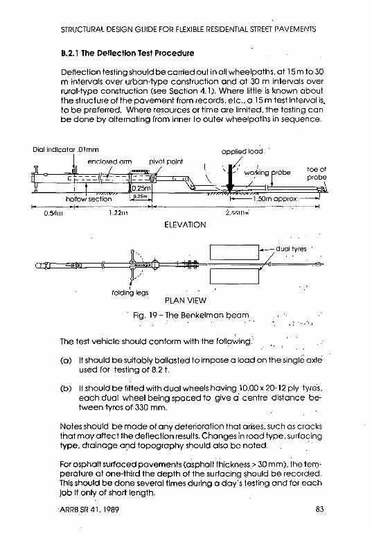
STRUCTURAL DESIGN GUIDE FOR FLEXIBLE RESIDENTIAL STREET PAVEMENTS
B.2.1 The Deflection Test Procedure
Deflection testing should be carried out in all wheelpaths, at 15 m to 30 m intervals over urban-type construction and at 30 m intervals over rural-type construction (see Section 4.1). Where little is known about the structure of the pavement from records, etc., a 15 m test interval is, to be preferred. Where r~sources or time are limited, the testing can be done by alternating from inner to outer wheelpaths in sequence.
Dial indicator .Olmm
l p.nr.losed arm
'1-0.54111 1..22111
pivot point I \
ELEVATION
PLAN VIEW
applied load / I I
, j wo;king probe
2. 1I4111 m
.=
Fig. 19 - The Benkelman I?earn .. j \ ' •• ~''''·.I
The test vehicle should conform with the following.'
(a) It should be suitably ballasted to impose a load on the single axle' used for testing of 8.2 t.
(b) It should be fitted with dual wheels having 10.00 x 20-12 ply tyre's, each dual wheel being spaced to give a' centre distance between tyres of 330 mm.
Notes should be made of any deterioration that arises, such as cracks that may aftect the deflection results. Changes in road type, surfacing type, drainage ar}d topography should also be noted. .
. . ' .
For asphalt surfaced pavements (asphalt'thickness > 30 mm), the ten)perature at one-third the depth of the surfacing should be record.ed. This should be done several times during a day's testing and for each job If only of short length.
ARRB SR 41, 1989 83

STRUCTURAL DESIGN GUIDE FOR FLEXIBLE RESIDENTIAL STREET PAVEMENTS
B.2.2 Corrections for Temperature and Moisture
For pavements with asphalt surfaces more than 25 mm thick. some allow<;:mce should be made for the effect of temperature on recorded deflections. The usual practice is to adjust deflections to a standard temperature (To) so that all deflections ore multiplied by a factor which depends upon the asphalt layer thickness (t) in mm and the difference between the test temperature and the standord temperature (T - TO> in °C. For example. the Department of Main ROads. NSW (1983) uses the temperature correction factors given in Table XVII. These temperature correction factors can be used when local figures ore not available. It is strongly recommended that the designer use correction factors which have been compiled as relevant to the particular region.
TABLE XVII
APPROXIMATE FACTORS TO BE APPLIED TO DEFLECTIONS TO CORRECT FOR SURFACE TEMPERATURE AS PER DMR NSW MR FORM 76 (1983)
(T -TO>°C To =25OC t (rnrn)
-15 -10 -5 5 10 15
30 0.95 0.97 0.98 1.02 1.03 1.05 40 0.94 0.96 0.98 1.02 1.04 1.06 50 0.92 0.95 0.97 1.03 1.05 1.08 60 0.91 0.94 0.97 1.03 1.06 1.09 70 0.89 0.93 0.96 1.04 1.07 1.11
/NB,: Table XVII should be corrected so that (T-To) is·1 read as (To-T) ._ .
If at all possible. pavements should be tested in their most critical moisture condition. that being:
during September to January in the southern part of Australia. or
during January to May in the northern part of Austrolia.
If they ore not. a correction for moisture must be introduced. such as that adopted by the Department of Main Roads. NSW (1983) (see Table XVIII ). Again it is strongly recommended that the designer develop his own correction factors for moisture as a function of subgrade soil type. rainfall and drainage conditions existing atthe site.
If the total width of pavement exists In a saturated condition. then the correction for moisture should be applied to all wheelpaths; otherwise. it should be applied to the outer wheelpath only.
84 ARRB SR 41. 1989

STRUCTURAL DESIGN GUIDE FOR FLEXIBLE RESIDENTIAL STREET PAVEMENTS
TABLE XVIII
APPROXIMATE FACTORS TO BE APPLIED TO DEFLECTIONS TO CORRECT FOR MOISTURE AS PER DMR NSW MR FORM 76 (1983) .
Rainfall (R in mm)
R ~ 75/J mm 75/J < R ~ 1200 mm R> 1200mm Water-Table < 3 m
(1) Winter. Spring rain
Sept to Jan (1) Jan to May (2)
1.0 1.0 1.0 1.0
(2) Summer rain
Deflection Test at Time or Year
Feb to Aug (1) June to Dec (2)
1.3 1.45 1.60 1.0
B.2.3 Determination of Characteristic Deflectlon(s)
After the necessary corrections for temperature and moisture have been made. deflections should be plotted. with results from each wheelpath identified separately. Such plots should enable one to Judge how the test length should be divided into homogeneous units on the basis of structural strength. Significant changes in. deflection should be apparent. --' .-.: •. -: .' .~ ~~ ". . .,
.. r'" . ~. . A further subdivision of these structural units may become necessary after consideration Is given to any noted changes in pavement condition. pavement type. surfacing type and/or traffic.
Within any homogeneous unit. at least ten deflection results should be available from each wheelpath.
Each homogeneous unit should be treated separately for the purposes of overlay design. with a characteristic deflection calculated for each wheelpath*.
·N.B. If same exceptionally high deflections and the road conditions indicate the need for patching prior to overlay. account should be taken of this by disregarding these deflections In the computation of the wheelpath characteristic deflection value.
ARRB SR 41. 1989 85

STRUCTURAL DESIGN GUIDE FOR FLEXIBLE RESIDENTIAL STREET PAVEMENTS
The formula to be used is as follows:
where d x s f
'f
d=:=.x+fs
the characteristic deflection (mm), the mean defledion (mm), the standard deviation of deflections (mm),and I.U tor an upper bound confidence IIrnil or 84 per cent, or 1.65 for an upper bound confidence limit ot 95 per cent.
The value adopted for f should correspond to the degree of reliability required in the overlay treatment: a valu~ of f = 1.0 provides good reliabilitY, while a value of f = ·1.65 provides excellent reliability. Consideration could be given to using f = 1 for local access and minor roads, and f;' 1.65 for. distributor and collector roads.
The highest characteristic deflection of all wheelpath values then becomes the deflection (dm) value representing the structural strength of the homogeneous unit concerned; and the need for overlay strengthening is judged on the basis of comparing this value (d.,) with the unit's tolerable deflection.
·B.3 DETERMINATION OF TOLERABLE DEFLECTION
The deflection obseNed atthe road surface when a wheel load passes is the sum of component deformations in the various pevement layers and in the subgrade. When this deflection exceeds a tolerable value (d,), the strain in the pavElm/:3nt or the subgrade reaches such a level that large permanent deformation can be transmitted through to the surface and failure can ensue. The objective, therefore, is to keep actual deflections. (or the greater percentage of them) below the tolerable value and so constrain permanent surface deformations to an acceploble level.
Tolerable deflection is known to be a function of not only traffic .Ioading, but also of pavement type and of surfacing type. For example, unbound materials are able to withstand greater deflections than bound materials because of their greater flexibility and likewise bituminous seals are able to withstand greater deflections than asphalt.
Table XIX indicates how tolerable deflection should be varied according to street type, depending on pavement structure (bound versus unbound) and pavement surfacing (asphalt versus bituminous seal) ..
86 AI~I~~ sr~ 41. 1989

STRUCTURAL DESIGN GUIDE FOR FLEXIBLE RESIDENTIAL STREET PAVEMENTS
TABLE XIX
TOLERABLE DEFLECTION AS A FUNCTION OF ROAD TYPE AND PAVEMENT TYPE (Mulholland 1986)
Bound Unbound Pavement Rood ESA/day Pavement Type Asphalt Bituminous
Seal
Distributor 40-380 0.65 1.00 1.20 Collector 10-150 0.80 1.25 1.45 Local Access 0.4-30 1.00 1.70 1.85 Minor 0.1-10 1.20 2.05 2.20
The need for pavement strengthening is judged on the basis of comparing the maximum characteristic deflection (dm) with the value of tolerable deflection (d,) as taken from Table XIX and the extent of asphalt overlay determined as per the procedure outlined in Section 8.4.
B.4 EXTENT OF ASPHALT OVERLAY
Taking each homogenous unit in turn, the procedure for determining the thickness of asphalt overlay is as follows:
(a) Ascertain whether dm > d,; if it does, then decide on the design life In years for the pavement to be overlaid.
(b) Estimate the design traffic loading in terms of cumulative ESA (refer Section 3.3).'
(c) Select the design (tolerable) deflection from the estimat~d design traffic loading; Fig. 20 shows the design deflection (dd) as a function of cumulative ESA for both bound and unbound pavements.
(d) Determine the overlay thickness required to reduce dm to ddby plotting (dm - dd) versus dm on Fig. 21
This procedure is simple, but several important points must be kept in mind.
• When an overlay is needed, the minimum thickness used should be2Smm.
• In normal fixed level construction, where the required overlay thickness exceeds 50 mm, reconstruction rather,than asphalt overlay may be the preferred treatment.
ARRB SR 41, 1989 87

STRUCTURAL DESIGN. GUIDE FOR FLEXIBLE RESIDENTIAL STREET PAVEMENTS
3.0
, 2.~
2.0
Tolerable deflection 1.5
(mm) I----~---
- u~bound pavement
I -- bound pavement -
---------- - -- ~ 1.0 --- -----.... 0.5
o 103
5xl0J
10'
5xl04 5xl0S
10'
Traffic: ESA
Fig. 20 - Design (tolerable) deflection as a function of cumulative ~SA for both bound and unbound pavements (Mulholland I(86) 1
1.5 r------,------.------,.-------,r-------,
en ,
(!:'<$' ~
1.0 1-----+----+--'---+---- 09';1'~'------"~ Reduction in ><i.~v~<;' deflection 1\O~
dm-dd 0.,)0\
(mm)
0.0 '----'---'--'--L--'---'---'-----'---'-....L--'---'-....L...L....-'--L-.-L........JL........J---J'--'--'---'-.....
88
0.5 1.0 1.5 2.0 2.5
Maximum characteristic deflection dm (mm)
Fig. 21 - Overlay design CUNes for residential street pavements (Mulholland 1986)
3.0
ARRB SR 41, 1989
10"
STRUCTURAL DESIGN GUIDE FOR'FLEXIBLE RESIDENTIAL STREET PAVEMENTS
• Before any overlay is placed, areas of failed pavement should be excavated and replaced with basecourse asphalt.
• Milling prior to overlaying may be a consideration where an Irregular surface exists, or where surface (oxidation) cracking prevails.
• To achieve good overall compaction, each layer comprising the overlay should have a thickness within the limits of one to three times the nominal aggregate dimensions.
• The contract specification should be written.(and construction control exercised) to ensure that the design overlay thickness occurs uniformly across the width of the pavement.
• After several weeks trafficking,. the completed overlay should be tested to check that the design criteria have in fact been satisfied; where they have not, redesign may be warranted, leading to the placement of an additional overlay.
8.5 EXAMPLE PROBLEM ILLUSTRATING OVERLAY DESIGN PROCEDURE
The following problem illustrates the previously-outlined procedure given in Sections B.2 to B.4.
The worked example relates to a pavement of fixed level construction which Is due for rehabilitation treatment. The street, Armstrong Avenue, Is shown to be located in the municipality of Brisbane, because Brisbane City Council is one Local Government Authority known to have developed its own temperature and moisture correction factors (Jones and Mallon 1983).
DATA:
Street Description
Subgrade
Pavement
Surfacing
Age of Pavement
ARRB SR 41, 1989
Local Access of 360 m length.
Mottled clay in first 210 m. . Yellow sandy clay in second 150 m.
200 mm consisting of unbound materials.
Spray seal plus reseal.
18 years.' "

STRUCTURAL DESIGN GUIDE FOR FLEXIBLE RESIDENTIAL STREET PAVEMENTS
Pavement Condition
Rainfall
Drainage
Topography
Truffic
Average Commercial Vehicle Count over three 24 hour days
Design Life of Asphalt Overlay
Signs of failure between Ch. 55 and Ch. 65. Some isolated signs of distress in first 170 m; otherwise appears in good structural condtlon.
1000 mm annually.
Good with.subsoil drains provided along entire length.
Flat.
450 veh/d present day.
3 empty light vans. 5 50% loaded light vans. 4 full light vans. 2 empty two-axle heavy trucks. 3 50% loaded two-axle heavy trucks. 2 full two-axle heavy trucks.
15 years.
Recorded deflections as per Figs 22 a to d.
DESIGN CALCULATIONS:
(j) Correction factors to be applied to recorded deflections are . as follows:
Temperature correction
Moisture correction.
1.00 (for spray seal*)
Highest Summer Deflection
Lowest Winter Deflection
1.25 (for good drainage sites)
• Brisbane City Council only opplies temperature corrections to asphalt surfaces exceeding 70 mm in thickness.
90 ARRB SR 41. 1989
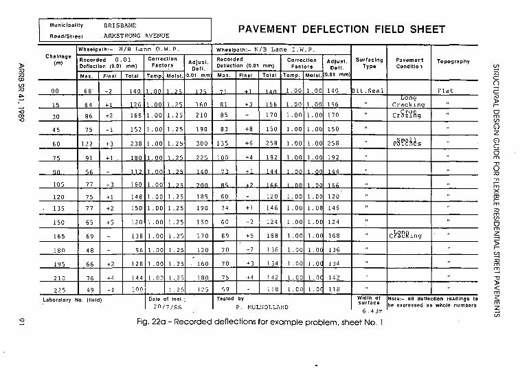
I Municipality BRISBANE PAVEMENT DEFLECTION FIELD SHEET RoadlStreet ARMSTRONG AVENUE
Chalnago (m)
00
15
30
45
60
75
qO
105
120
135
150
165
180
195
210
225
laboratory
Wheelpath:- NIB Lane O.W.P. Wheelpath:- NIB Lane I .W. P.
Recorded 0.01 Correction Recorded Correction Surlaclng Adjust. Adjust. Oelloctlon (0.01 mm) Factors
Dell. Oellectlon (0.01 mm) Factors Doll. Typo
Max. Final Tolal TemD Moist. :0.01 mm Max. Final Total Temp. Moist .0.01 mm)
68' -2 140 11 . on 11 ? '; 17<; 7 .1 In 1. 00 1. 00 140 bit.Sea1
64 +1 126 1. 00 1. 25 160 81 +3 156 1. 00 1. 00 156 "
86 +2 168 1. 00 1. 25 210 85 - 170 1. 00 1. 00 170 "
75 -1 152 1. 00 1. 25 190 83 +8 150 1. 00 1. 00 150 "
In +3 238 1. 00 1. 25 300 135 +6 258 1. 00 1. 00 258 "
91 +1 180 1. 00 1. 25 225 100 +4 192 1. 00 1. 00 192 "
'iii 112 11.00 I. 25 140 7' .1 1 d d 1 _ 00 1 _ O~ 144 "
77 -3 160 1. 00 1 ? <; ?OO R<; +? 1hh 1 nn 1 nr 1hh "
75 +1 148 1. 00 1. 25 185 60 - 120 1. 00 1. 00 120 "
77 +2 150 1. 00 1 .. 25 190 74 +1 146 1. 00 1. 00 146 "
65 +5 120 1. 00 1. 25 150 60 -2 124 1 .00 1. 00 124 "
69 - 138 1. 00 1 .25 170 89 +5 168 1. 00 1. O~ 168 "
48 - 96 1.00 1.25 120 70 +2 136 1. 00 1.0C 136 "
-66 +2 128 1. 00 1. 25 160 70 +3 134 1.00 1.0 134 "
76 +4 144 1.00 1.25 180 75 +4 142 1. 00 1.0 142 "
49 -] 10(,1 I .25 125 59 - 118 1.01) I. a lIS "
No. (lield) Tested by Width 01 surface I [)a~o 01 test:
.0/7/86 P. MULHOLL/,ND 6.43m
Fig. 22a - Recorded deflections for example problem, sheet No.1
Pavemert Conditio'
Topography
Flat Long
Cr"cki.na "
cr~2~gg "
"
p§~~Ms "
.,
"
"
"
"
"
d~B~inq "
"
"
"
" Note:- all de-flection readings to be expressed as whole numbers
~ ;;v C () -; C ;;v » r o m en G) Z G) c a m
" o ;;v
" r m X OJ r m ;;v m en a m Z -; » r
~ ;;v m m -;
~ m s: m Z ill
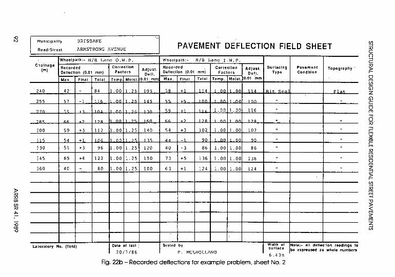
I I i
.. BRISBI\NE Municipality
PAVEMENT DEFLECTION FIELD SHEET Road/Slreel ARMSTRONG I\V:::NUE
Wheelpath:- NIB Lane O.W.P. Wheelpalh:- NIB Lane I.W. P. I
C,.lnage Recorded Correction Recorded Correctl~n Adjust. ! Surfacing
(m) Deflection (0.01 mm) Factors
Adjust. Deflecllon (0.01 mm) Factors Type Defl. Defl.
Max. Final Tolal Temp. Moist. 0.01' mm Max. Final Total Temp. Moist. 0.01 inm
240 42' - 84 1. 00 1. 25 105 58 +1 114 1,00 1 .00 114 B't Spa
255 57 -1 116 11 nn 1 JS 14S ~S ,S 1nn 1 nn nn ,nn "
~7n SS .1. 1 nA nn ,~ 1n 59 +1 11<. 1. 00 1. 00 116 "
"R~ /;/; ,? l?R nn 11 ?~ /;n <.<. ,7 7R nn nn ?R .. ;00 59 +3 112 1.00 1. 25 140 54 +3 102 1. 00 1. 00 102 "
,15 'i4 +1 1 nn .nn 1 7'i 11'i 44 -1 90 1..J10 1 00 90 "
;30 51 +3 96 1.00 1. 25 120 40 -3 86 1. 00 1. 00 86 "
;:45 65 +4 122 1. 00 1. 25 150 73 +5 136 1. 00 1.00 136 "
360 40 - 80 1. 00 1. 25 100 63 +1 124 1. 00 1. 00 124 "
La,oralory No. (field) Oato of test : lested by Widlh of surface
20/7/86 P. MULHOLLAND 6.43m
Rg. 22b - Recorded deflections for example problem, sheet No.2
Pavement Topography' Condition
F'l .. ~
"
"
"
"
"
"
"
Note:- all deflec"ion readings to be expressed as whole numbers
~ ;v c Q c ~ r o m (f>
G) Z (j) c a m -n
~. -n r m X 05 r m ;v
rn a m Z -f
5> r
~ ;v m m -f
~ m ~ m Z u:J

I Municipality BRISBANE PAVEMENT DEFLECTlON FIELD SHEET Road/Str"et
Chalnage (m)
00
15
30
45
60
75
90
105
120
135
150
165
180
195
210
225
Laboratory
ARMSTRONG AVENUE
Wheelpath:- SIB Lane O.W.P. Wheelpath:- "fR '" T W D
Recorded Correction Recorded Correctloll Adjust. Surfacing Deflection (0.01 mm) Factors Adjust.
Deflection (0.01 mm) Factors Type Defl. Defl.
Max. Final Total Temp Moist. 0.01 mm Max. Final Total Temp. Morst. 0.01 mm)
84· +4 160 1. 00 1. 25 200 80 +3 154 1. 00 1.llO 154 Bit Sea
84 +1 166 1. 00 1. 25 210 78 +3 150 1. 00 1.no 150 "
73 +3 140 11.00 11.25. 175 hR ,~ 1?" nn r n I?" "
94 +3 182 11.00 II ?~ ??~ 00 - ,.,0 nn 'n 17R "
139 +5 268 1. 00 1. 25 335 130 +5 250 1. 00 1. (,0 250 "
76 - 152 1. 00 1. 25 190 104 -1 210 1. 00 1. 00 210 "
70 +8 124 1. 00 1. 2: 155 75 +4 142 1. 00 11.(0 142 "
75 +2 146 1. 00 1 .2" 185 qR - 1Q" 1 nn r.n 1Q" "
71 +4 114 ~OO +..2" -L6S. '0 -" ,n nn I, r"<n 160 "
73 +3 140 .00 ll~ ~ fiO +1 114 1 00 (\(\ 114 "
54 -1 110 00 1 ~? S 140 ,,0 I' n nn I, (VI 110 "
77 +1 152 1. 00 1. 25 190 80 +2 156 1. 00 1. 0:) 156 "
74 +2 144 1. 00 1. 25 180 66 -1 134 1.00 1. OJ 134 "
51 -2 106 1. 00 1. 25 130 90 - 180 1. 00 1. 0) 180 "
70 +6 128 1.00 1 .25 160 7? - 144 nn 11 n1 1. "
43 +3 80 1.00 1 .25 100 4? +? RO 100 1 0:1 Rn " No. (field) Date of test: Tested by Widlh 01
sUlfaco 20/7/36 P. ~WLHOLL,\ND
6.43rn
Fig. 22c - Recorded deflections for example problem, sheet No.3
PaverT'ent Topography Condition
Flat Lona
Cracki~ "
"
" ",rnaJ.J. Patches "
,-roc Crazinq "
"
"
"
"
" "ong
Cracki~g "
"
"
"
" Note: all ::Jefleclion readings to be expressad as whole numbers
~ Al C () -I C Al » r-o m Vl G) Z (j) c a m
(5 Al
" r-m X OJ rm Al
m a m Z -I » r-
~ Al m m -I
~ m S m Z ul

» ;;V ;;V OJ (J) ;;V
l>.
-0 CD -0
I 'Aunicipality BRISBANE
I PAVEMENT DEFLECTION FIELD SHEET Road/Street ARMSTRONG AVENUE
Wheelpath:- S/B' Lane O. W. P .. Wheelpath:- S/B Lane I.W. P. Ch.lnage
Recorded ;m) Deflection (0.01 mm)
Max. Final Total
240 60 -2 124
,,55 44 - 68
;;70 51 +1 100
;;85 47 +2 90
:00 51 3 108
,:15 40 +2 76
110 54 InR
345 65 +4 122
360 59 +5 108
Labor.tory No. (field)
Correcllon Recorded Correction, Adjust. Surfacing Factors Adjust.
Deflection (0.01 mm) Factors Dell. Type Deft. Temp Moist. 0.01 mm PJlax. Final Total Temp. Moist. 0.01 mm)
1. 00 1. 25 155 6J +4 112 1. 00 1. 00 112 Bit.Sea
1. 00 1. 25 85 5:) - laO 1. 00 1. 00 100 .. 1. 00 1. 25 125 59 +4 110 1. 00 1. 00 110 ..
1. 00 1. 25 115 48 +1 q4 11 .00 1 no q4 ..
1.001 25 115 7h +1 114 h 11 . no 1 .00 14h .. 1.0 1. 25 ...9.5 ...5.4 - 110R 11 .00 1 .00 lOR ..
1 .O( .2S 11S 6:1 _1 1,,,, nn n '''' .. 1. 00 1. 25 150 56 -4 120 1. 00 1. c·o 120 ..
1. 00 1. 25 135 75 +3 144 1. 00 1. 00 144 ..
tt. st ~ of. .r· In :> or
f.' '"h n ,er' ,n '7°,..
Cate oj test Tesled by Width 01 surface
20/1/86 P. ~lULHOLL)l.ND 6.43m
Rg. 22d - Recorded deflections for e>:ample problem. sheet NO.4
Pavement Topography Condition
Flat
..
..
..
..
..
.. "
"
Nole:- all deflection readings to be expressed 3S whole numbers
~ ;;v c () -< c ~ r o m (J)
(j) z (j) c o m
o ;;v
" r m X CD r m ;;v m (J)
o m Z -< » r
~ ;;v m m -<
~ m ~ m Z (jj
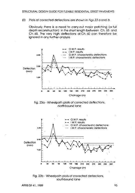
STRUCTURAL DESIGN GUIDE FOR FLEXIBLE RESIDENTIAL STREET PAVEMENTS
(ii) Plots of corrected deflections are shown in Figs 23 a and b.
Obviously. there is a need to corry out major patching (or full depth reconstruction) in the short length between Ch. 55 and Ch. 65. The very high deflectidns at Ch. 60 can therefore be Ignored In any further analysis.
Deflection (mm)
3.00
2.00
1.00
O.W.P. results I.W.P. results O.W.P. characteristic deflections I.W.P. characteristic deflections
I ! I , , ..
o 30 60 90 120 150 180 210 240 270 300 330 360
Chainage (m)
Fig. 23a - Wheelpath plots of corrected deflections. riorthboundlane
J.UU
2.00
Deflection (mm)
1.00
O.W.P. results I.W.P. results O.W.P. characteristic deflections I.W.P. characteristic deflections
o 30 60 90 120 150 180 210 240 270 300 330 ~60
Chainage (m)
Fig. 23b - Wheelpath plots of corrected deflections. southbound lane
ARRB SR 41. 1989 95

STRUCTURAL DESIGN GUIDE FOR FLEXIBLE RESIDENTIAL STREET PAVEMENTS
The wheelpath plots indicate that the street length should be broken up into two homogenous units: .
Unit 1 - Ch. 00 to Ch. 210, and Unit 2 - Ch.·210 to Ch. Jm ..
Other data (Le. pavement condition and subgrade type). confirm this to be the correct break-up.
Characteristic deflections (CDs) can then be determined as per the summary given in Table XX.
TADL[ X)(
WORKED OVERLAY DESIGN EXAMPLE; SUMMARY OF DEFLECTION STATISTICS
Homogenous. Lane and Wheel path Unit
Unit No: 1 Northbou'nd OW.P Northbound IW.P . Southbound I.W.P Southbound O.W.P
Unit No.2 Northbound O.w.P NOnnOOUM I.W.I-' Southbound I.W.P Southbound O.w.P
Mean x (mm)
1.75 1.49 1.54 1.77
1.31 1.11 1.14 1.23
From the above Table, it can be taken that:
for Unit 1, dm = 2.20 mm; and for Unit 2, d~ = 1.61 mm.
S.D C.D <! (mm) x + 1.65cr
0.27 2.20 0.18 1.79 0.28 2.01 0.25 2.19
0.18 1.61 U.14 1.34 0.20 1.47 0.22 1.60
These figures can be contrasted with the tolerable deflection value (d,) drawn from Table XIX.
• For an unbound pavement with bituminous seal. constructed as a local access road, d, = 1.85 mm.
The conclusion, therefore, is that Unit 1 requires an asphalt overlay, while Unit 2 does not.
96 ARRB SR 41. 1989

STRUCTURAL DESIGN GUIDE FOR FLEXIBLE RESIDENTIAL STREET PAVEMENTS
(iii) Design Traffic
Ns
Y
Design Traffic
Design Deflection (dd)
Design Overlay ThlolmmG
N,.365.Y
(3 x 0.0001 + 5 x 0.0008 + 4 x 0.028 + 2 x 0.19 + 3 x 0.6 + 2 x 2.15) ... 2 3.42 (Section 3.3.2)
16.2 (frUIII Tublt:: VI)
3.42 x 365 x 16.2 20186, say, 2.0 x 10· ESA. .
1.95 mm (Fig, 20)
2.20 - 1.95 = 0.25
25mm (Fig. 21)
.. '
In this particular instance, the decision would probably be made to apply an overlay thickness of 25 mm throughout the street length, including both Units 1 and 2. This would overcome any potential problem brought on by a change in surfacing type. It could also be used as a preventative rt:laintenance measure, costing relatively little for the additional pavement life achieved.
ARRB SR 41. 1989 97

ARRB PUDLICAJIONS
Th" Auslralian Road Research I:loard publishes a large numberoflechnical reports and manuals. A list of the most recent is shown below.
14th ARRB Conference Proceedings, Parts 1-8
Special Report No. 39 'Development of ·techniques for studying unsafe driving actions' by K.D. Charlesworth and P.T. Cairney
ipoolill naport tlo. 40 'Development and evaluation of highway speed weigh-in-motion oyztems in Australia' by S.E. Samuels
Special Report No. 42 'A history of traffic engineering in Australia' by R.T. Underwood
ARRB Research Report No. 154 'Speeds, friction factors and alignment design standards' by J.R. McLean
ARRB ReSto .. r~h Report No. ISS 'VLlMITS: an expert system for speed zone determination in Victoria' by J.R. Jarvis and C.J. Hoban
ARRB Research Report No. 156 'A citation analysis of Australian road technology' by M.G. Lay
ARRB Research Report No. 158 'Performance of eTB p"VAmRnt~ IIn(i",r lIr.t:olllratlld loading. Tho Quocn~· land ALF trial. 1986/87' by P. Kadar, E. Baran and R.G. Gordon
ARRB Technical Manual No. 26 'Description and operation of the ARRB video traile( by J.S. Dods
ARRB Technical Manual No. 27 'Prediction of traffic noise at simple signalised intersections' by S.E. Samuels and H. !:>hepherd
Order for these and olher ARRB publieatlons can be sent to:
Australian Road Research Board, PO Box 156, Nunawadlng, 3131, Victoria, Australia Telephone: (03) 235 1555 Fax: (03) 233 8878