a study into the optimisation and calculation of electrical losses in
TRANSCRIPT
Department of Mechanical and Aerospace Engineering
A study into the optimisation and calculation of
electrical losses in renewable energy generation
Author: Chris McGee
Supervisor: Dr Nick Kelly
A thesis submitted in partial fulfilment for the requirement of the degree
Master of Science
Sustainable Energy: Renewable Energy Systems and the Environment
2014

2
Copyright Declaration
This thesis is the result of the author’s original research. It has been composed by the
author and has not been previously submitted for examination which has led to the
award of a degree.
The copyright of this thesis belongs to the author under the terms of the United
Kingdom Copyright Acts as qualified by University of Strathclyde Regulation 3.50.
Due acknowledgement must always be made of the use of any material contained in,
or derived from, this thesis.
Signed: Date: 05/09/2014

3
Abstract
This project will investigate the main causes of electrical losses in renewable energy
generation.
The financial backers of many of the renewable projects being constructed today are
primarily concerned with achieving maximum profitability for their clients. One of
the key losses of revenue for a renewable energy project is ongoing losses from the
electrical components. It is therefore essential that we can accurately predict
electrical losses before investment. Investors need accurate, bankable data pre
construction and during site acquisition phases.
Firstly, a review of the losses attributed to the electrical technologies involved in
renewable energy generation will be conducted. This will involve performing an
analysis of empirical data from a variety renewable energy projects.
This data will then be used to construct tool for quickly and accurately predicting
losses in future projects thus giving potential investors bankable data for their
investments.

4
Acknowledgements
I would like to take this opportunity to thank the following people who helped in an
academic, support or social way throughout this project and the culmination of my
MSc.
I would like to thank my supervisor Dr. Nick Kelly who gave guidance and direction
on the technical aspects of this thesis.
Special thanks to SgurrEnergy for providing loss data for the project and for giving
me the opportunity to enhance my electrical career.
Special thanks go to the Electrical team at SgurrEnergy who helped formulate my
ideas. Especially David Partington for his assistance with fine tuning the loss tool.
A big thanks to all my fellow students who made this course one of the most
enjoyable and fulfilling experiences I’ve had so far. I made some genuine new
friends here.
I am grateful for the support of my family who has always believed in me no matter
what. I couldn’t have done this without them.
And finally to Rebecca. This one is for you.

5
Contents 1. Introduction .......................................................................................................... 10
1.1. Background ................................................................................................... 10
1.2. Objectives ...................................................................................................... 11
1.3. Scope ............................................................................................................. 11
1.4. Methodology ................................................................................................. 11
2. Technology ........................................................................................................... 13
2.1. Renewable energy systems............................................................................ 13
Solar Photovoltaic................................................................................................. 13
Onshore Wind ....................................................................................................... 16
Offshore Wind ...................................................................................................... 18
2.2. Electrical equipment ...................................................................................... 20
Cables ................................................................................................................... 20
Transformers ......................................................................................................... 23
Inverters ................................................................................................................ 25
3. Review of losses ................................................................................................... 27
3.1. Electrical Losses ............................................................................................ 27
Cable Losses ......................................................................................................... 27
Transformer Losses .............................................................................................. 29
Inverter Losses ...................................................................................................... 30
3.2. Data acquisition ............................................................................................. 32
4. Loss Tool .............................................................................................................. 35
4.1. Software specification and design ................................................................. 35
4.2. Development of tool ...................................................................................... 35
Input Parameters ................................................................................................... 35
Assumptions and exclusions ................................................................................. 40
4.3. Verification.................................................................................................... 41
Model testing ........................................................................................................ 41
5. Case study ............................................................................................................. 44
5.1. Technical review ........................................................................................... 44
5.2. Results ........................................................................................................... 47
6. Conclusions .......................................................................................................... 48

6
7. Further Work ........................................................................................................ 49
8. References ............................................................................................................ 50

7
List of Figures
Figure 2-1Solar Photovoltaic layout (Alasdair Miller, 2010) ...................................... 14
Figure 2-2 Typical site layout ...................................................................................... 17
Figure 2-3: Offshore wind farm arrangement .............................................................. 18
Figure 2-4 HV Power and control cables (Maximum HDMI Cable Length) ............. 20
Figure 2-5: ABB offshore cable ................................................................................... 21
Figure 2-6 Schneider Electric Minera range Tx datasheet (http://www.schneider-
electric.com/downloads) .............................................................................................. 24
Figure 2-7 Inverter configurations (Alasdair Miller, 2010) ......................................... 25
Figure 2-8 Transformer and transformerless inverter configuration (Alasdair Miller,
2010) ............................................................................................................................ 26
Figure 3-1 Stranded cable (Moore, 1999) .................................................................... 28
Figure 3-2 Miliken Conductor cross section (associates) ............................................ 29
Figure 3-3Freesun HEC-UL Inverter characteristics (Electronics, 2013) ................... 31
Figure 3-4 Inverter efficiencies (Alasdair Miller, 2010) ............................................ 32
Figure 4-1 Tab definition ............................................................................................. 42
Figure 5-1 Case Study Windfarm layout ..................................................................... 45

8
List of Tables
Table 1 Common cable parameters(Moore, 1999) ...................................................... 23
Table 2 Windfarm 1 operational report data ................................................................ 33
Table 3 Cable data aquisition ....................................................................................... 34
Table 4 Transformer data aquisition ............................................................................ 34
Table 5 Plant definition input ...................................................................................... 37
Table 6 Array cable input ............................................................................................ 38
Table 7 Transformer Input ........................................................................................... 39
Table 8 Array cable input ............................................................................................ 39
Table 9Case Study array cable arrangement ................................................................ 45
Table 10 Case study operational data .......................................................................... 46
Table 11 Case Study availability ................................................................................. 46
Table 12 Case study loss calculation results ................................................................ 47

9
Abbreviations and Acronyms
Abbreviation or Term Definition
AC Alternating Current
Ampacity Electrical current carrying capacity
Capex Capital Expenditure
DC Direct Current
DNO Distribution Network Owner
DRS Dynamic Rating System
DTS Distributed Temperature Sensing
HVAC High Voltage Alternating Current
HVDC High Voltage Direct Current
HV/MV/LV High Voltage / Medium Voltage
LTDS Long Term Development Statement
MPPT Maximum power point tracking
MVA Mega Volt Amperes
MVAr Mega Volt Amperes reactive
MW Mega Watts
OFTO Offshore Transmission Owner
OHL Overhead Line
ONAN Oil Natural Air Natural
Opex Operational Expenditure
OTDR Optical Time Domain Reflectometry
OWF Offshore Wind Farm
RTTR Real Time Thermal Rating
SCADA Supervisory Control and Data Acquisition
TSO Transmission System Operator
WTG Wind Turbine Generator
XLPE Cross Linked Poly Ethylene
10
1. Introduction
1.1. Background
The purpose of this thesis is to investigate the electrical losses in renewable energy
generation across several renewable generation technologies. Only the losses
encountered between point of generation and the metering connection point will be
considered as these are key to the bankable data which investors and developers
require to make informed financial decisions. These investors and developers use
renewable energy consultancies such as SgurrEnergy to provide the technical
expertise to back up their financial knowledge and allow them to make informed
choices about their investments.
Renewable energy generation projects are generally financed through a project
finance approach. Equity and project finance investment groups typically conduct a
project evaluation covering the legal aspects, permits, contracts, technical and
financial aspects. These are evaluated prior to achieving the projects financial close.
Projects are evaluated through Legal, Insurance and Technical due diligence
processes. The technical due diligence process concentrates on the following aspects:
Sizing of the generation plant (MW).
Physical layout of the site.
Electrical design layout and sizing.
Technology review of the major components.
Energy yield assesments.
Contract assessments
Financial model assumptions
SgurrEnergy perform many professional services for investors and developers
throughout the lifecycle of a renewable project. Some of these services include
performing this due diligence and energy yield analysis.
11
SgurrEnergy and especially the electrical department are frequently asked about the
electrical losses expected from a renewable energy generation project. To ensure
good value for clients the electrical team requires an easy to use and accurate loss
prediction method.
1.2. Objectives
The objective of this thesis is to undertake an analysis of the electrical losses
encountered in renewable energy generation and create an accurate prediction tool
that can be used to inform clients and investors. This thesis will document the process
that will enable the electrical team to provide bankable information on electrical
losses quickly and accurately while providing good value for both SgurrEnergy and
the Client. These loss calculations will then be able to be integrated into due
diligence or energy yield reports for other departments for submission to the Client.
Loss data and energy yields from existing renewable energy generation projects will
be collected and used to test the validity of the loss prediction tool.
The tool will be constructed in excel and will be an easy to use interface with multiple
input options. These will include Cable type, transformers and solar components such
as inverters and combiner boxes. Different renewable technologies such as solar
photovoltaic, onshore and offshore wind will be included in the loss calculation tool
as these make up the bulk of SgurrEnergy’s current portfolio.
1.3. Scope
The tool will be constructed upon mathematical models taken from first principle
electrical loss calculations. The tool will have to be accurate across various different
parameters for it to be admissible as bankable data for investors and developers. Only
components that contribute to a significant electrical loss will be factored in to the
model.
This thesis takes loss data from established projects in several worldwide locations
within SgurrEnergy’s extensive portfolio. The generation voltages vary as do the
generating technologies and size and location of the projects.
1.4. Methodology
A literature review was conducted on relevant published articles, working groups,
presentations, brochures, equipment specifications and industry papers. These are to

12
be reviewed to give an understanding of the past and recent developments in the field
of electrical losses.
An indicative loss calculation model will be constructed in Microsoft Excel and is
aimed at providing an illustrative approach to the electrical losses expected over a
range of renewable generation options.
Actual loss data from renewable generation plants within the SgurrEnergy portfolio
will be analysed and compared to the tool results to ensure accuracy across all the
renewable technologies.
A case study on a renewable energy generator will be conducted and its actual
measured electrical output compared to the calculated output determined by the loss
calculation tool.
This will give an indication of the tools accuracy.
13
2. Technology
Renewable energy generation comes in many forms and Scotland is lucky to
be situated geographically to take advantage of all of them with the exception
of Solar which would be better implemented in sunnier climates further south.
SgurrEnergy with their global footprint are ideally placed to consult across the range
although Scotland still makes up a significant portion of their renewable portfolio.
Renewables by their nature can be intermittent in their operation. In general for
renewable generation, export power varies as the wind speed or solar irradiation
across the site fluctuates. This creates a variable loading pattern on the power
transmission and distribution equipment connecting the site to the electrical grid. The
loading pattern associated with the output from renewable energy fluctuates and
cannot be controlled in the same way as more traditional embedded generation.
Electrical equipment is typically selected with appropriate static ratings to support the
maximum export current (MVA) requirements (both steady state and transient fault
current) however the maximum export capacity may only be realised for a fraction of
the site operating profile.
2.1. Renewable energy systems
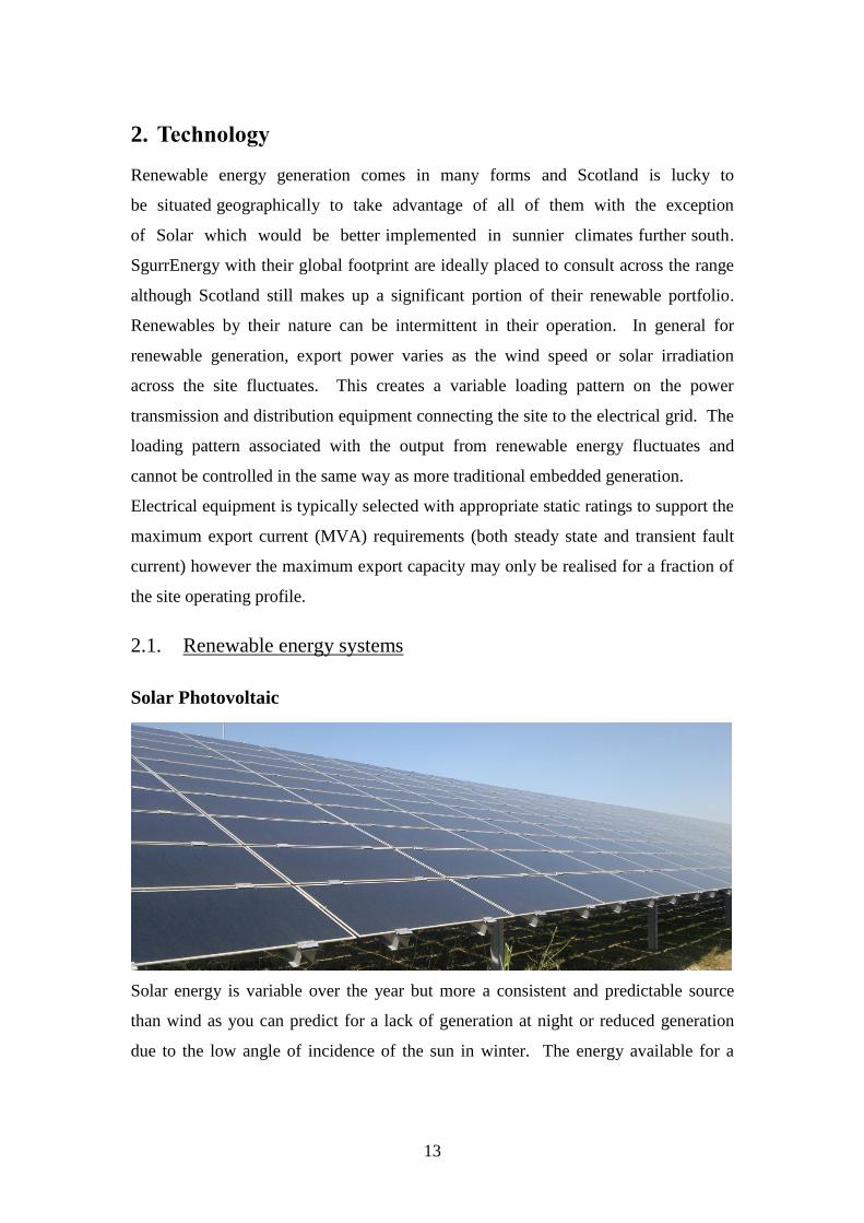
Solar Photovoltaic
Solar energy is variable over the year but more a consistent and predictable source
than wind as you can predict for a lack of generation at night or reduced generation
due to the low angle of incidence of the sun in winter. The energy available for a

14
solar installation is defined by the global horizontal irradiation which is the total
surface energy received on a unit area of receiving surface.
Thermal and voltage impacts on the DNO network are as per other embedded
generation within these periods of generation.
Inverters in photovoltaic generation need to be maintained near to full load capacity to
operate in their most efficient zone. Therefore it is common practice for inverters to
be undersized by 20% of the installed peak capacity, thus operating in the high
efficiency zone. This increases power delivery throughout the year, with only some
losses in high summer due to the undersizing. It has been shown in studies that the
conceptual design of a solar photovoltaic plant and the positioning of the inverters and
combiner boxes can have a dramatic effect on copper losses (Papastergiou, 2010)
The electrical design of a photovoltaic generation site is split between DC and AC
systems.
Figure 2-1Solar Photovoltaic layout (Alasdair Miller, 2010)
The DC system is made up of the following:
Array(s) of PV modules.

15
Inverters.
DC cabling (module, string and main cable).
DC connectors (plugs and sockets).
Junction and combiner combiners.
Disconnects and switches.
Protection devices.
Earthing.
The AC system is made up of the following:
AC Cabling.
Switchgear.
Transformers.
Substation.
Earthing and surge protection.
Solar photovoltaic modules have non-linear output efficiency due to environmental
effects such as shadowing and hot spots, electrical tolerances and different power
output across cells, so MPPT is employed to smooth power delivery by using
algorithms to sample power output and then alter the load across the string. These are
normally included in the inverter hardware and so the output of the whole string is
optimised based on the average.
There have been studies conducted in relation to PV plant design suggesting losses
can be reduced by increasing the DC collector grid before step up to AC (Siddique,
2014), however it is the experience of the author that this technique is not in
widespread use in the industry and is at an early stage of investigation.
Solar plants by their nature have a lower availability than wind generation so their
output is measured by a solar plants performance ratio. This is normally shown as a
percentage and is used to compare solar farm against each other. The performance
ratio quantifies the overall losses on the rated output of a solar plant.

16
Onshore Wind
Onshore wind has been a significant influence in SgurrEnergy’s entry into the
renewable consultancy business. It is fitting as Scotland led the world in the
development of electrical generation from wind, in fact the first wind powered
electrical generator was built by Professor James Blyth in Scotland in 1887 (Price,
2005). With Scotland’s windy climate it is natural that it should harness this abundant
resource for its power generation needs. This is the case at the moment and Scotland
has seen a rapid rise in recent years in the amount and scale of on shore wind farms
being erected around the country and currently 60% of renewable energy is
generated from wind farms both on shore and offshore. Whitelee windfarm in south
west Scotland is the biggest onshore windfarm in Europe consisting of 140 turbines
and generating a peak of 322MW of electricity (www.whiteleewindfarm.co.uk/about).
With this rapid expansion has come criticism. Wind turbines, initially seen as elegant
and futuristic have now become viewed eyesores in some quarters, ruining
Scotland’s scenic heritage in the eyes of many and pressure is now mounting to
develop large scale offshore capability instead of onshore. However transmission
and implementation costs for offshore generation rise considerably. Scotland does
have extensive offshore pipeline and cabling experience due to the oil industry and it
is hoped that this will drive costs down along with government renewable obligation
certificates (ROC’s). Unfortunately Scotland’s early lead in wind turbine

17
development wasn’t protected at government level and that lead was lost to
Denmark who now lead the world in technology implementation and
development. This should be an incentive to not make the same national
mistakes regarding offshore wind power development.
Onshore wind typically consists of a smaller number of turbines than offshore.
Whitelee as discussed has over 100 turbines but typical installations are 10-20
turbines. Turbine outputs vary but maximum onshore turbine size is normally 3 MW
due to local environment and planning issues.
Projects consist of ring or radial circuits of WTG’s with their own transformers and
switchgear stepping up the generation voltage to the site array voltage. This is then
fed back via the site array to the site substation for connection to the distribution grid
as shown in Figure 2-2
Figure 2-2 Typical site layout
These sites can take up a wide geographic area with cable runs into the tens of
kilometres and so losses can be significant due to the large distances between the
outlying WTG’s and the export metering point.
Onshore wind farm electrical components consist of the following:
WTG
WTG Transformer
Array cable
Switchgear
Export Transformer

18
Electrical losses will be recorded at all of these stages.
Offshore Wind
As the technology of wind generation has been optimised and up scaled, not to
mention the permitting and social pressures being felt by the onshore wind industry,
large scale offshore wind developments have witnessed a rapid rise to prominence and
focus.
Offshore developments are becoming larger in scale. Not only are the number of
turbines and arrays increasing in size, but the individual turbines are becoming larger
with Vestas unveiling its 8 MW turbine prototype (www.renewable
energyworld.com)
Figure 2-3 provides an overview of a typical UK offshore wind project and the
boundaries of responsibility for the stakeholders involved in the construction and
operation of a renewable energy connection to the electrical grid.
Figure 2-3: Offshore wind farm arrangement
With the larger distances involved in transmission from turbine to turbine and from
the offshore substations, transmission losses through the cable may be increased.
Offshore developments may mitigate for this by increasing the array voltages from 33
kV to 66 kV is some cases and by utilising HVDC technology at the offshore
substation. The increase in costs for the capital expenditure can be significant for
both the individual turbine 66 kV step up transformers and HVDC substations so any
19
generation losses that can be saved by utilising these technologies must be able to
offset these costs.
Electrical equipment in offshore environments is traditionally specified for continuous
power ratings however it is known that electrical equipment such as cables and
transformers may operate at higher ratings for periods of time. Under variable
operating load conditions the temperature of the equipment is allowed to rise then
cool as the load increases and decreases. In these situations it may be possible to
apply a dynamic rating to equipment which may enable greater power export through
electrical equipment.
Dynamic rating is a term that is applied to extending the rating of electrical equipment
in operation for periods of minutes, hours or days depending on the requirement and
constraints. It is essentially a decision to ‘overload’ electrical assets based on the
knowledge that the equipment can withstand the overload period and magnitude.
Dynamic ratings have been applied by electrical network operators for many years
and are based on the experience of the operator and their knowledge of the equipment.
An operator may choose to knowingly allow the overload of a circuit in the network
for an acceptable period to maintain availability. This is commonly known as
“sweating” an electrical asset.
More recently dynamic ratings have been applied using information from temperature
monitoring systems to enable the application of more accurate, continuous and
measured ratings on electrical equipment, this is referred to as a real time thermal
rating (RTTR).
The output of a RTTR system can theoretically be automatically integrated into the
power control system however this is considered a potential future development once
operators are comfortable with the feedback from a RTTR system philosophy.
In all cases overloading will increase the electrical losses to increased temperatures in
the equipment but may be offset against potential losses due to curtailment of
generation.
20
2.2. Electrical equipment
Cables
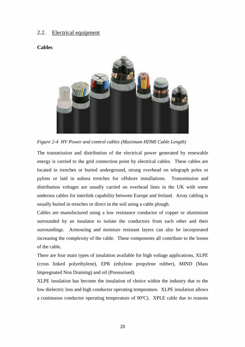
Figure 2-4 HV Power and control cables (Maximum HDMI Cable Length)
The transmission and distribution of the electrical power generated by renewable
energy is carried to the grid connection point by electrical cables. These cables are
located in trenches or buried underground, strung overhead on telegraph poles or
pylons or laid in subsea trenches for offshore installations. Transmission and
distribution voltages are usually carried on overhead lines in the UK with some
undersea cables for interlink capability between Europe and Ireland. Array cabling is
usually buried in trenches or direct in the soil using a cable plough.
Cables are manufactured using a low resistance conductor of copper or aluminium
surrounded by an insulator to isolate the conductors from each other and their
surroundings. Armouring and moisture resistant layers can also be incorporated
increasing the complexity of the cable. These components all contribute to the losses
of the cable.
There are four main types of insulation available for high voltage applications, XLPE
(cross linked polyethylene), EPR (ethylene propylene rubber), MIND (Mass
Impregnated Non Draining) and oil (Pressurised).
XLPE insulation has become the insulation of choice within the industry due to the
low dielectric loss and high conductor operating temperature. XLPE insulation allows
a continuous conductor operating temperature of 90ºC). XPLE cable due to reasons

21
of market availability, potential impacts on the environment and ease of installation is
the most common type cable encountered in renewable energy generation.
For the higher transmission voltages required for large scale offshore generation,
higher capacity subsea cables are used. Insulation voltages of up to 150 kV are now
becoming more common in three-core subsea XLPE cable applications. Transmission
voltages up to 170 kV are not uncommon however and they represent the established
end of the solid dielectric HV cable market. There is currently limited experience
above this voltage level.
Submarine cables provide the means to collect and export power from the offshore
WTGs to the wider grid onshore. In offshore wind farm installations there are two
types of submarine cable:
Inter Array Cables.
Export Cables.
Inter array cables provide a collection system which connect the individual WTGs to
the offshore substation while the export cables provide the connection from the
offshore substation to the shore where there typically is a connection to a land based
cable. Both types of cable are usually 3 core type with copper conductors, XLPE
insulation and integral optical fibres as shown in Figure 2-5.
Figure 2-5: ABB offshore cable
Inter array cabling usually operates at 33 kV or 66 kV while export cables operate at
voltages in excess of 100 kV.
Three-core submarine cables are available up to 245 kV using a solid dielectric
(XLPE), and a number of wind farms under development have orders for cables rated
for this voltage. This level of technology has limited service history and is still under
development
22
There is a history of self-contained fluid filled insulated cables (a form of pressurised
oil) being used for 400kV+ AC submarine cables but these are rare in the industry.
Losses in cables occur due to heat being dissipated when the cables are energised and
under load. Cable losses can be split into Conductor losses, dielectric losses and
sheath losses.
In solar photovoltaic applications low voltage DC is determined by national grid
codes and regulations determined applicable to that country.
According the IFC solar guidebook, solar cable should meet the following criteria.
The cable voltage rating. The voltage limits of the cable to which the PV
string or array cable will be connected must be taken into account.
Calculations of the maximum Voc voltage of the modules, adjusted for the site
minimum design temperature, are used for this calculation.
The current carrying capacity of the cable. The cable must be sized in
accordance with the maximum current. It is important to remember to de-rate
appropriately, taking into account the location of cable, the method of laying,
number of cores and temperature. Care must be taken to size the cable for the
worse case of reverse current in an array.
The minimisation of cable losses. The cable voltage drop and the associated
power losses must be as low possible. Normally, the voltage drop must be less
than 3%, but national regulations must be consulted for guidance. Cable
losses of less than 1% are achievable. (Alasdair Miller, 2010)
Cables for power generation are manufactured to recognised standards to ensure
operational quality is met regardless of installation conditions. These standards
include but are not limited to:
BS 60228 Conductors of Insulated Cables
IEC 60287 Electric Cables – Current Rating
IEC 60840 Power Cables with extruded installation and their accessories
23
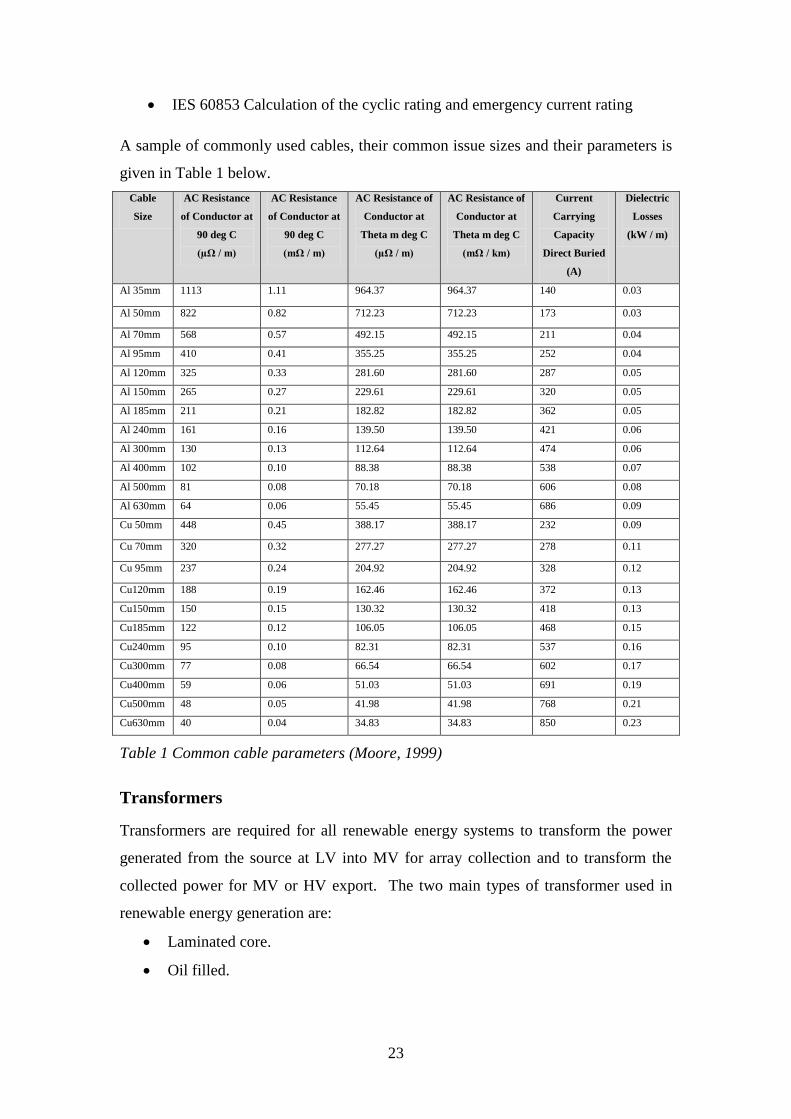
IES 60853 Calculation of the cyclic rating and emergency current rating
A sample of commonly used cables, their common issue sizes and their parameters is
given in Table 1 below.
Cable
Size
AC Resistance
of Conductor at
90 deg C
(µΩ / m)
AC Resistance
of Conductor at
90 deg C
(mΩ / m)
AC Resistance of
Conductor at
Theta m deg C
(µΩ / m)
AC Resistance of
Conductor at
Theta m deg C
(mΩ / km)
Current
Carrying
Capacity
Direct Buried
(A)
Dielectric
Losses
(kW / m)
Al 35mm 1113 1.11 964.37 964.37 140 0.03
Al 50mm 822 0.82 712.23 712.23 173 0.03
Al 70mm 568 0.57 492.15 492.15 211 0.04
Al 95mm 410 0.41 355.25 355.25 252 0.04
Al 120mm 325 0.33 281.60 281.60 287 0.05
Al 150mm 265 0.27 229.61 229.61 320 0.05
Al 185mm 211 0.21 182.82 182.82 362 0.05
Al 240mm 161 0.16 139.50 139.50 421 0.06
Al 300mm 130 0.13 112.64 112.64 474 0.06
Al 400mm 102 0.10 88.38 88.38 538 0.07
Al 500mm 81 0.08 70.18 70.18 606 0.08
Al 630mm 64 0.06 55.45 55.45 686 0.09
Cu 50mm 448 0.45 388.17 388.17 232 0.09
Cu 70mm 320 0.32 277.27 277.27 278 0.11
Cu 95mm 237 0.24 204.92 204.92 328 0.12
Cu120mm 188 0.19 162.46 162.46 372 0.13
Cu150mm 150 0.15 130.32 130.32 418 0.13
Cu185mm 122 0.12 106.05 106.05 468 0.15
Cu240mm 95 0.10 82.31 82.31 537 0.16
Cu300mm 77 0.08 66.54 66.54 602 0.17
Cu400mm 59 0.06 51.03 51.03 691 0.19
Cu500mm 48 0.05 41.98 41.98 768 0.21
Cu630mm 40 0.04 34.83 34.83 850 0.23
Table 1 Common cable parameters (Moore, 1999)
Transformers
Transformers are required for all renewable energy systems to transform the power
generated from the source at LV into MV for array collection and to transform the
collected power for MV or HV export. The two main types of transformer used in
renewable energy generation are:
Laminated core.
Oil filled.

24
WTG Transformers are provided to transform the LV output from the source into MV
for collection in the array network. Transformers are typically rated to meet the
source capacity and are located close to the generation source. In WTG’s,
transformers can be located in turbine, either in the nacelle, the base or outside, in
offshore WTG’s these can be located in the transition pieces of the offshore WTG
structure. Solar PV transformers are located next to the inverters in bays throughout
the solar farm.
Export transformers are required to transform the power from the array voltage to a
higher export voltage for transmission to the grid. As these are required to export a
significant amount of power from the whole generating plant they are usually much
larger with larger potential for losses.
Transformer ratings and characteristics are given in the manufacturers transformer
datasheet as shown in Figure 2-6
Figure 2-6 Schneider Electric Minera range Tx datasheet (http://www.schneider-
electric.com/downloads)
Transformers associated with large scale renewable projects are typically oil
insulated. Typically this provides a certain capability to operate in an overloaded
condition for a period before thermal breakdown of the windings and insulation
occurs. The heating and cooling of transformers is generally slower than with cables,
therefore any rating ‘bottle neck’ is more associated with cables.
Power transformers are typically sized to carry the maximum continuous MVA rating
of the project. Particularly for oil immersed transformers that are mostly used in
renewable energy projects, it is common to allow a period of overload, sometimes up
to 150% of continuous rating (depending on cooling system and insulation class).

25
This can often justify the under-sizing of transformers to save on size and cost which
are both important factors in offshore projects where space and cost savings are of
significant benefit.
Under-sizing of export or WTG transformers for rated output is not typical practice
for wind projects. Export transformers are known to be sized to utilise short term
overload capability in the event of outages. Therefore there is usually significant
short term overload capability in these components.
The life expectancy of transformers, regulators and reactors at various operating
temperatures is not accurately known. A typical transformer is guaranteed for the full
lifetime of the project, which can range from 20 to 30 years.
IEC 60076-7 (Loading guide for oil-immersed power transformers) may be used to
give an indication of permissible daily loading duties. This IEC standard can also be
applied to transformer design when considering the variable nature of renewable
energy generation.
Inverters
Inverters are used in renewable energy generation mainly in photovoltaic applications.
The inverters are used to convert DC into AC for stepping up to grid distribution and
transmission voltages.
Figure 2-7 Inverter configurations (Alasdair Miller, 2010)
In photovoltaic applications, inverters may be string type or central type. Central
inverters are used in medium to large photovoltaic installations typically over 5 MW.
String inverters are typically used in photovoltaic installations under 10 MW but as
pricing becomes more competitive they are becoming more prevalent.
26
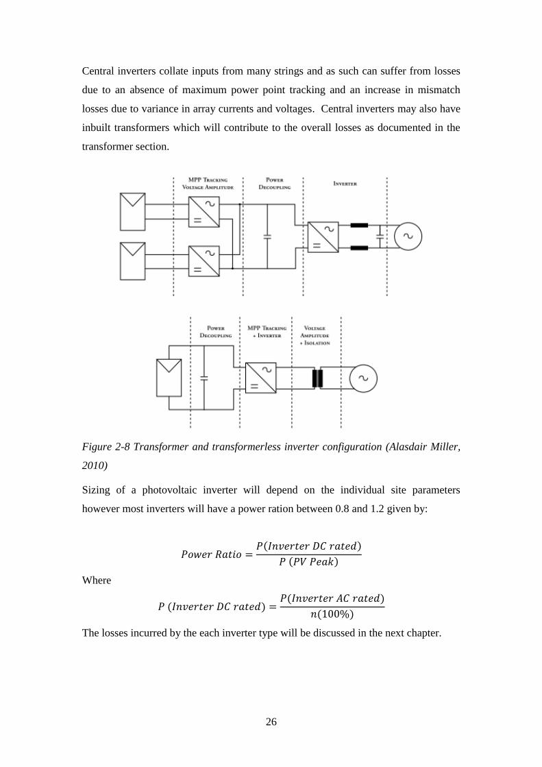
Central inverters collate inputs from many strings and as such can suffer from losses
due to an absence of maximum power point tracking and an increase in mismatch
losses due to variance in array currents and voltages. Central inverters may also have
inbuilt transformers which will contribute to the overall losses as documented in the
transformer section.
Figure 2-8 Transformer and transformerless inverter configuration (Alasdair Miller,
2010)
Sizing of a photovoltaic inverter will depend on the individual site parameters
however most inverters will have a power ration between 0.8 and 1.2 given by:
( )
( )
Where
( ) ( )
( )
The losses incurred by the each inverter type will be discussed in the next chapter.
27
3. Review of losses
3.1. Electrical Losses
Electrical losses occur due to many factors in renewable energy generation depending
on the technology being utilised.
Ancillary System or parasitic losses are due to parasitic consumption within the
generating facility. This may include losses for heaters or cooling systems,
transformer no-load losses, safety equipment and control systems.
Grid compliance control losses can be due to limitations on the grid external to the
renewable generator, both due to limitations on the amount of power delivered at a
given time, as well as limitations on the rate of change of power deliveries. These
could also include losses due to the power purchaser electing to not take power
generated by the wind due to curtailment conditions detailed in the grid connection
agreements between the generator and the DNO.
The electrical transmission efficiency including WTG transformers, solar inverters,
collection wiring, substation transformers and transmission wiring will be reviewed as
part of this study.
Cable Losses
Losses in electrical cables, whether they are onshore, offshore, buried or overhead
line occur when the load on the cable generates heat in the various constituent parts.
These consist of the conductor cores, the dielectric, any outer metallic layers or
shielding and any external insulation.
The conductor losses are ohmic losses given by:
nI2Rθ (watt)
Where n = number of cable cores
I = Current carried by the conductor (Amps)
Rθ= ohmic a.c. resistance of the conductor at θoC (Ω)
During the transmission of high A.C., the skin effect and proximity effect ensure that
the current is not evenly distributed throughout the cross section of the conductor.
The skin effect occurs when the cable is constructed from a large number of
concentric circular elements such as a stranded cable shown in Figure 3-1 .

28
Figure 3-1 Stranded cable (Moore, 1999)
The strands at the centre of the cable are surrounded by more strands and as such are
subjected to a greater magnetic flux than those strands on the outside of the cable.
This causes the current density to be greater on the outside of the cable than it is at the
centre. The increase in current density results in an increase in conductor resistance
which in turn will contribute to the overall losses.
The proximity effect also contributes to overall cable losses. In this instance
overlapping magnetic fields between closely arranged conductors interact via their
respective magnetic fields.
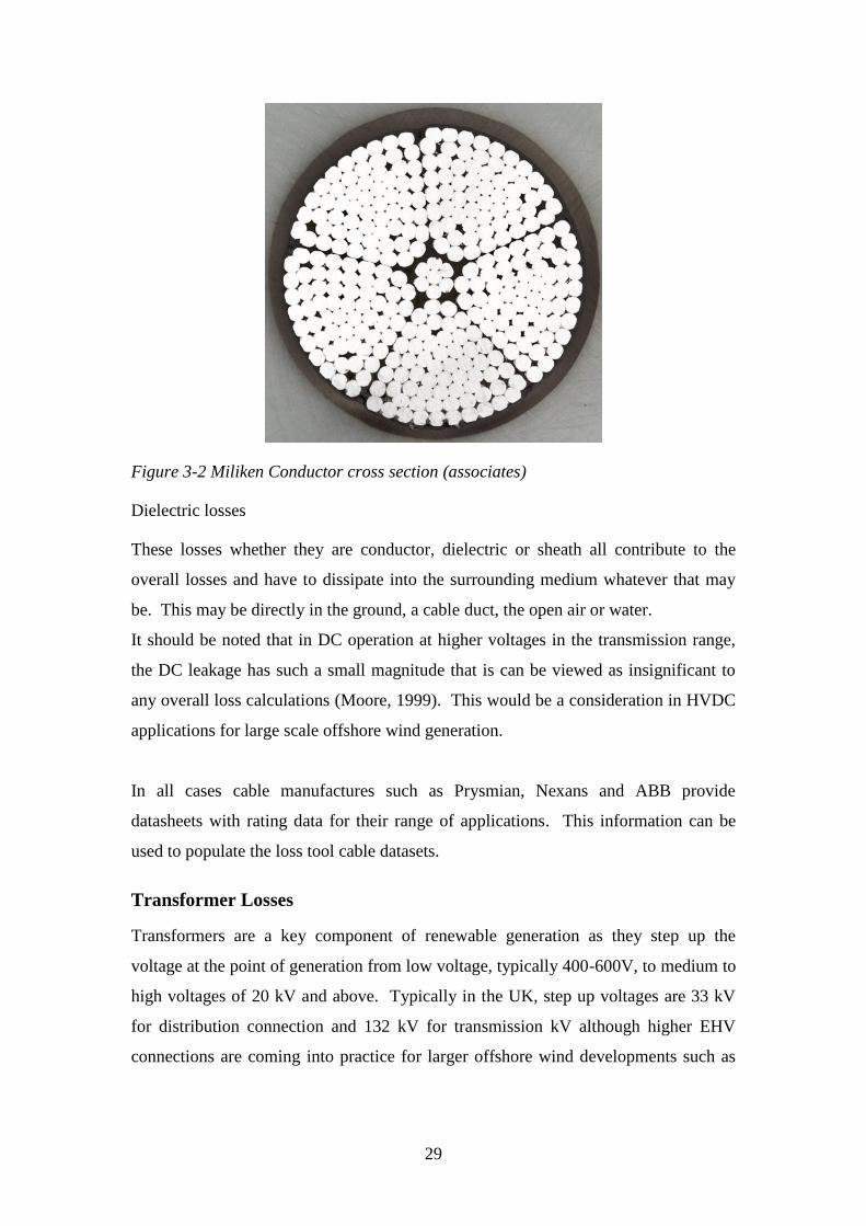
In both cases these losses and effects can be reduced by innovative cable design and
conductor arrangement and shaping. One such design is the milliken conductor which
uses shaped groups of conductors to reduce the effects.
29
Figure 3-2 Miliken Conductor cross section (associates)
Dielectric losses
These losses whether they are conductor, dielectric or sheath all contribute to the
overall losses and have to dissipate into the surrounding medium whatever that may
be. This may be directly in the ground, a cable duct, the open air or water.
It should be noted that in DC operation at higher voltages in the transmission range,
the DC leakage has such a small magnitude that is can be viewed as insignificant to
any overall loss calculations (Moore, 1999). This would be a consideration in HVDC
applications for large scale offshore wind generation.
In all cases cable manufactures such as Prysmian, Nexans and ABB provide
datasheets with rating data for their range of applications. This information can be
used to populate the loss tool cable datasets.
Transformer Losses
Transformers are a key component of renewable generation as they step up the
voltage at the point of generation from low voltage, typically 400-600V, to medium to
high voltages of 20 kV and above. Typically in the UK, step up voltages are 33 kV
for distribution connection and 132 kV for transmission kV although higher EHV
connections are coming into practice for larger offshore wind developments such as
30
London array which has two offshore substations exporting via two Nexans 150 kV
XLPE submarine export cables (www.nexans.com/news)
As previously discussed the higher the export voltage, the less the transmission,
export and distribution losses will be over the length of the cable. Depending on the
circuit configuration, the metering point of the generation plant is likely to be on the
export side of the metering switchgear after the step up transformer. This means that
any losses before this point will be part of the site electrical losses.
Transformers are subject to losses in both the core and the windings. The current
required for magnetising the core in order for it to cycle the magnetic flux at the
system frequency dissipates energy. This is commonly known as the no load loss.
This occurs whenever the transformer is energised.
Load losses also occur whenever there is a flow of current in the system. This is
determined by the magnitude of the current and the resistance of the system. This is
especially marked in the transformer windings. These losses only occur when the
transformer is under load. (Heathcote, 2008)
These losses are given as part of the manufacturers’ datasheets and along with the
efficiency and transformer ratings can be input into the loss tool datasets as tool is
expanded. It should be noted that forced cooling by either oil or air flow can reduce
the temperature of the windings. This allows the transformer to either operate at a
higher rating or the temperature losses can be reduced.
Inverter Losses
Inverter losses in Solar PV are a smaller contributer to the overall loss calculation
than either the cables or transformers. As most inverters are transformerless, the
losses are concentrated on the semiconductor components of the inverter circuitry.
These losses are ususlly in the order of 95% with peak efficiency od up to 98% in
transformerless inverters (Luo, 2013). Inverter efficiency is measured according to
IEC 61683 to ensure compliance.
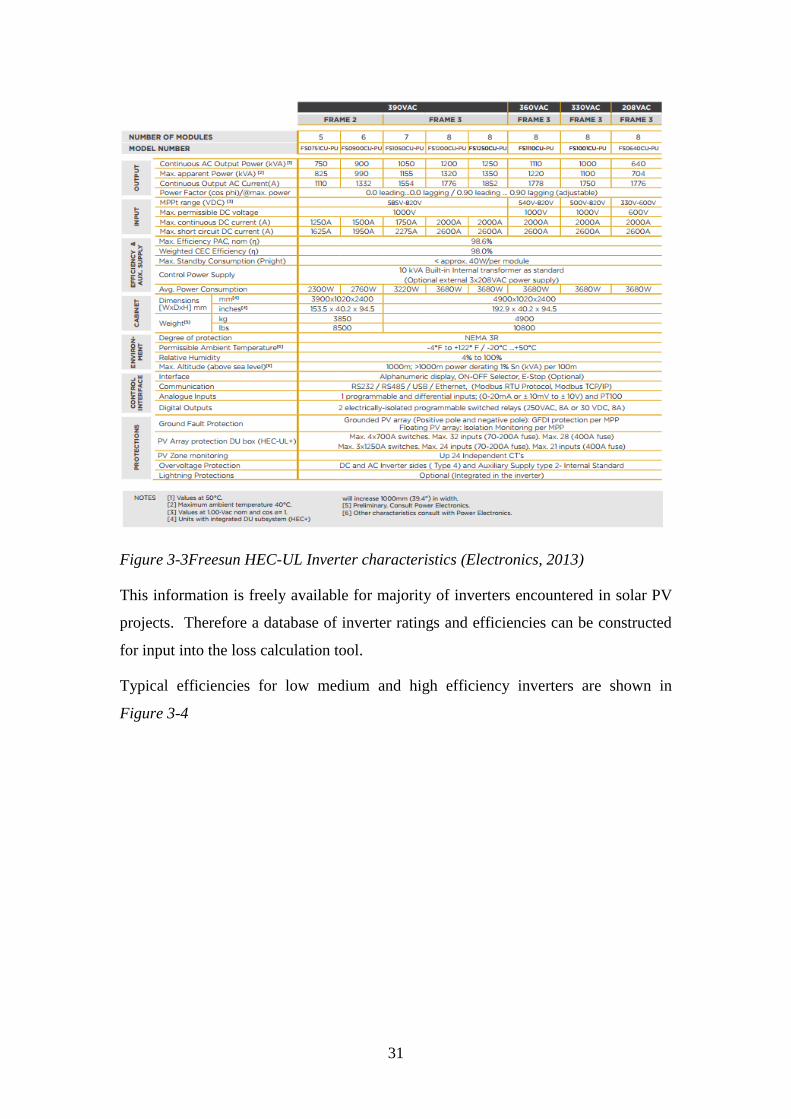
Datasheets provided publicly for inverters commonly used in solar PV generation
projects provide the efficiencies and ratings that may be used for calculations. The
datasheet and values for the Freesun HED-UL Central inverter are shown in Figure
3-3.
31
Figure 3-3Freesun HEC-UL Inverter characteristics (Electronics, 2013)
This information is freely available for majority of inverters encountered in solar PV
projects. Therefore a database of inverter ratings and efficiencies can be constructed
for input into the loss calculation tool.
Typical efficiencies for low medium and high efficiency inverters are shown in
Figure 3-4

32
Figure 3-4 Inverter efficiencies (Alasdair Miller, 2010)
Inverters are manufactured to ensure their efficiencies are in accordance with IEC
61683:1999 Photovoltaic systems – Power conditioners –Procedure for measuring
efficiency.
3.2. Data acquisition
Loss data has been acquired from SgurrEnergy’s large and varied portfolio. As
discussed, SgurrEnergy’s profile is wide and varied, however on and off shore wind
along with Solar PV make up the bulk of their business interests. To this end it was
decided to take three of the most used technologies along with three examples of each
of these to ensure a wide sample of loss data could be tested against the model.
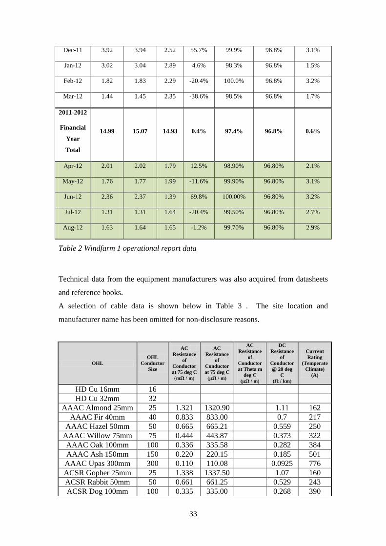
An example of an on shore wind farm operational report data is shown below in Table
2
Months
Energy
Exported1
(GWh)
Energy
Generated
(GWh)
Budget
Energy
(GWh)
Export
Variance2
(%)
Overall
Operational
Availability
(%)
Budgeted
Overall
Operational
Availability
(%)
Availability
Variance (%
points)
Oct-11 2.82 2.83 2.36 19.0% 95.5% 96.8% -1.3%
Nov-11 1.97 1.98 2.52 -21.6% 92.3% 96.8% -4.5%
33
Dec-11 3.92 3.94 2.52 55.7% 99.9% 96.8% 3.1%
Jan-12 3.02 3.04 2.89 4.6% 98.3% 96.8% 1.5%
Feb-12 1.82 1.83 2.29 -20.4% 100.0% 96.8% 3.2%
Mar-12 1.44 1.45 2.35 -38.6% 98.5% 96.8% 1.7%
2011-2012
Financial
Year
Total
14.99 15.07 14.93 0.4% 97.4% 96.8% 0.6%
Apr-12 2.01 2.02 1.79 12.5% 98.90% 96.80% 2.1%
May-12 1.76 1.77 1.99 -11.6% 99.90% 96.80% 3.1%
Jun-12 2.36 2.37 1.39 69.8% 100.00% 96.80% 3.2%
Jul-12 1.31 1.31 1.64 -20.4% 99.50% 96.80% 2.7%
Aug-12 1.63 1.64 1.65 -1.2% 99.70% 96.80% 2.9%
Table 2 Windfarm 1 operational report data
Technical data from the equipment manufacturers was also acquired from datasheets
and reference books.
A selection of cable data is shown below in Table 3 . The site location and
manufacturer name has been omitted for non-disclosure reasons.
OHL
OHL
Conductor
Size
AC
Resistance
of
Conductor
at 75 deg C
(mΩ / m)
AC
Resistance
of
Conductor
at 75 deg C
(µΩ / m)
AC
Resistance
of
Conductor
at Theta m
deg C
(µΩ / m)
DC
Resistance
of
Conductor
@ 20 deg
C
(Ω / km)
Current
Rating
(Temperate
Climate)
(A)
HD Cu 16mm 16
HD Cu 32mm 32
AAAC Almond 25mm 25 1.321 1320.90 1.11 162
AAAC Fir 40mm 40 0.833 833.00 0.7 217
AAAC Hazel 50mm 50 0.665 665.21 0.559 250
AAAC Willow 75mm 75 0.444 443.87 0.373 322
AAAC Oak 100mm 100 0.336 335.58 0.282 384
AAAC Ash 150mm 150 0.220 220.15 0.185 501
AAAC Upas 300mm 300 0.110 110.08 0.0925 776
ACSR Gopher 25mm 25 1.338 1337.50 1.07 160
ACSR Rabbit 50mm 50 0.661 661.25 0.529 243
ACSR Dog 100mm 100 0.335 335.00 0.268 390

34
ACSR Wolf 150mm 150 0.223 222.50 0.178 512
ACSR Lynx 175mm 175 0.191 191.25 0.153 562
ACSR Panther 200mm 200 0.165 165.00 0.132 615
ACSR Zebra 400mm 400 0.083 82.75 0.0662 931
Table 3 Cable data acquisition
A selection of the transformer data is shown below in Table 4. The site location and
manufacturer name has been omitted for non-disclosure reasons.
Power (MVA) Losses (kW) Voltage (kV)
ONAN ONAF NLL LL Total losses
8 10 8.5 63 71.5
12 15 10.5 74 84.5 38/20
12 15 38/20
16 20 12.5 85 97.5 38/20
24 30 38/20
31.5 40 22 177.37 199.37
48 60 110/20
60 24.5 240 264.5 110/20
60 75 29 259 288 110/20
75 27.5 280 307.5 110/20
70 88 42 345 387
80 100 38 423 461 110/20
80 100 110/20
80 100 47 190 237 110/20
100 33.5 335 368.5 110/20
84 112 138/34.5/313.8
90 120 38 423 461 110/20/10
Table 4 Transformer data acquisition

35
4. Loss Tool
4.1. Software specification and design
The tool has to be able to be used in an office environment primarily in the electrical
department at SgurrEnergy, but across departments and in the global offices if
required. This narrows down the software options somewhat. The author decided
that using a software package that required a paid licence would not be cost effective
and transference of data across departments would be problematic. Dedicated non
licenced software packages would remove the cost issue but there would be a training
aspect involved.
It was decided to use Microsoft Excel as the basis for the loss calculation tool as this
is readily available as part of the Microsoft office package installed on all the
SgurrEnergy computer systems across all the business departments and regions.
Microsoft Excel has the capability of storing multiple data sets. This is a requisite as
large amounts of cable, transformer and inverter data will be stored as a reference
within the tool.
This data will need to be pulled depending on the project technical parameters. Excel
allows this with the VLOOKUP function and tis inbuilt logic functions.
The tool has to be able to differentiate between different technologies and only pull
data that is relevant to that chosen technology.
This is performed with drop down menus on the front page. These are selectable with
the generation technology required. The parameters required for the chosen
technology then become available, all others being ignored.
Once all the required parameters and known inputs have been selected, the tool will
look up the datasets for the technical values and perform the calculation and show the
loss value as both a value and percentage of the total as required.
4.2. Development of tool
Input Parameters
The tool has been designed from the outset to be user friendly from the outset. This
requires input parameters to be relevant and easily identified.

36
Firstly the type of renewable generation technology is to be defined by the user. Each
technology will have different parameters linked to it for referencing. The
technologies included in this version of the tool are as follows:
Solar Photovoltaic
Onshore Wind
Offshore Wind
These three technologies represent 80% of SgurrEnergy’s current workload and as
such are relevant to the vast number of investor and due diligence queries regarding
electrical losses. The flexibility of the tool will ensure that more technologies can be
included as well as more datasets for the existing ones as new technology is
developed.
Each technology will have different input parameters that are exclusive to that type of
technology and will have stored datasets for the tool to access. A choice of one
particular technology will lock out parameters and datasets not relating to that
technology. This will keep the inputs and therefore calculations and outputs accurate.
Once the user has chosen the technology, the next stage will be to choose the number
of generating units. Depending on the application, these may be WTG’s or solar
inverters.
The inputs required for all technologies are as follows:
Technology Type
Number of generating units
Generating Unit rating (MW)
Maximum power factor setting
The Total rating is calculated by multiplying the unit rating by the number of units.
The Maximum MVA is given by dividing the total rating by the maximum power
factor.
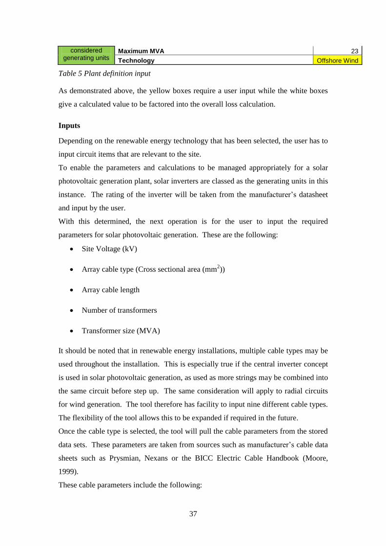
An example of the layout of the plant definition input section is shown in Table 5
PLANT GENERAL
DEFINITION - For Solar,
Inverters are
Unit rating (MW) 2
Number of generating units 11
Total Rating (MW) 22
Maximum Power Factor Setting 0.95
37
considered generating units
Maximum MVA 23
Technology Offshore Wind
Table 5 Plant definition input
As demonstrated above, the yellow boxes require a user input while the white boxes
give a calculated value to be factored into the overall loss calculation.
Inputs
Depending on the renewable energy technology that has been selected, the user has to
input circuit items that are relevant to the site.
To enable the parameters and calculations to be managed appropriately for a solar
photovoltaic generation plant, solar inverters are classed as the generating units in this
instance. The rating of the inverter will be taken from the manufacturer’s datasheet
and input by the user.
With this determined, the next operation is for the user to input the required
parameters for solar photovoltaic generation. These are the following:
Site Voltage (kV)
Array cable type (Cross sectional area (mm2))
Array cable length
Number of transformers
Transformer size (MVA)
It should be noted that in renewable energy installations, multiple cable types may be
used throughout the installation. This is especially true if the central inverter concept
is used in solar photovoltaic generation, as used as more strings may be combined into
the same circuit before step up. The same consideration will apply to radial circuits
for wind generation. The tool therefore has facility to input nine different cable types.
The flexibility of the tool allows this to be expanded if required in the future.
Once the cable type is selected, the tool will pull the cable parameters from the stored
data sets. These parameters are taken from sources such as manufacturer’s cable data
sheets such as Prysmian, Nexans or the BICC Electric Cable Handbook (Moore,
1999).
These cable parameters include the following:
38
Conductor CSA (mm2)
Insulation CSA (mm2)
Conductor resistance DC 20oC (Ω/km)
Conductor resistance AC 90oC (Ω/km)
Insulation resistance 20oC (Ω/km)
Capacitance (µF/mm)
Inductance (mH/km)
Current Rating (A)
MVA rating @ V (MVA)
Losses (W/m)
MVA rating for each cable is given by the following:
( )
Where A is the current rating and V is the array voltage.
Array Cable losses are then calculated by taking the stated cable losses for that type of
cable and multiplying by the length of cable.
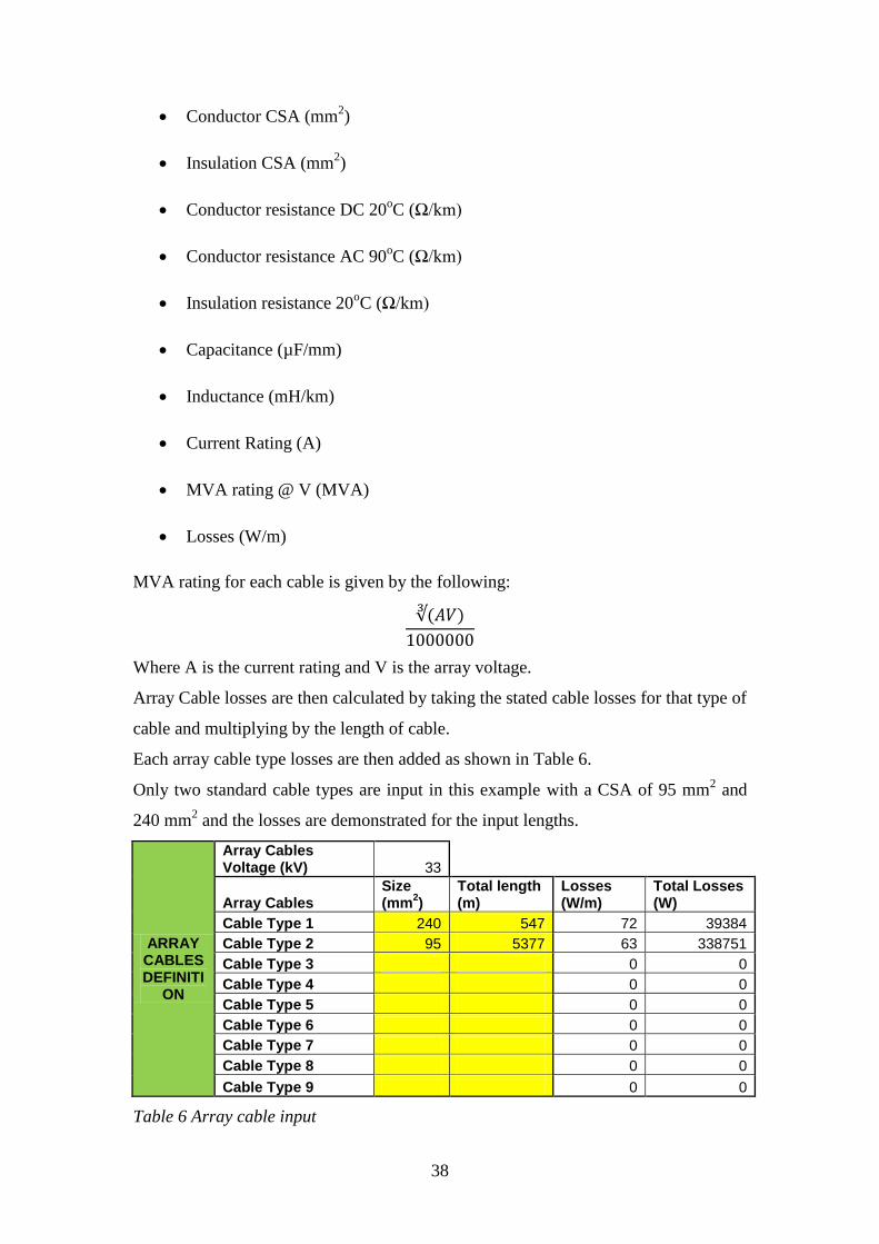
Each array cable type losses are then added as shown in Table 6.
Only two standard cable types are input in this example with a CSA of 95 mm2 and
240 mm2 and the losses are demonstrated for the input lengths.
ARRAY CABLES DEFINITI
ON
Array Cables Voltage (kV) 33
Array Cables Size (mm
2)
Total length (m)
Losses (W/m)
Total Losses (W)
Cable Type 1 240 547 72 39384
Cable Type 2 95 5377 63 338751
Cable Type 3 0 0
Cable Type 4 0 0
Cable Type 5 0 0
Cable Type 6 0 0
Cable Type 7 0 0
Cable Type 8 0 0
Cable Type 9 0 0
Table 6 Array cable input

39
Once the array cable losses are calculated the transformer losses are then determined.
Depending on the site configuration and layout design parameters, there may be
several stages of step up transformation performed. Typically in wind sites, WTG’s
have a transformer stage as well as the site having a transmission or distribution
transformer stage. Therefore there are input slots in place to be used by the operator
as required. In this way all transformer losses may be taken into account for the final
calculation.
These losses are determined by inputting first the number of transformers and their
MVA rating. The load losses (W) are then input by the user from the manufacturer’s
data sheets dependant on which make of transformer is being used.
The total losses can then be calculated by multiplying the individual load losses by the
number of transformers.
TRANSFORMERS
DEFINITION
Transformers Number
Size (MVA)
Load Losses (W)
Total Losses (W)
Transformer Type 1 (e.g. WTG) 11 2.1 16600 182600
Transformer Type 2 (e.g. Export Tx) 0 0 0 0
Transformer Type 3 0 0 0 0
Table 7 Transformer Input
The final loss calculation is performed on the export cable if required. The inputs are
shown in Table 8. There are a number of options as shown. The ability to choose AC
or Dc cable is available however the tool has not been equipped with the ability to
calculate these at this time and would be a development of the tool in time as this
becomes a more prevalent technology. The tool was designed to allow relatively easy
development if required.
EXPORT CABLE
DEFINITION
Export Cable AC
Number of Export Circuits 2
Export Cable Voltage (kV) 245
Total Export Current (A) 55
Current Per Circuit (A) 27
Export Cable length (m) 70000
Export Cable size (mm2) 630
DC Resistance of Export Cable Cores (per core) (ohms) 0.027
AC Resistance of Export Cable Cores (per core) (ohms) 0.036
AC Resistance of each circuit over export cable length (ohms) 7.565
Full load Losses on Export Cables (MW) 0.011
Table 8 Array cable input

40
Assumptions and exclusions
Typical cable data including current ratings and cable mass was taken from publically
available data published by BICC Cables (Moore, 1999). Specific values of cable
losses per km and costs for different cable sizes could not be provided by any cable
manufacturer as the information was described as commercially sensitive and project
specific.
Resistance of the export cables has been assumed as equal to the DC conductor
resistance (neglecting temperature rise) based on IEC 60287:
R'=ρ
R’ = DC conductor resistance
ρ = resistivity of conductor (1.7 x 10⁻⁸
for Copper)
l = Length of conductor
A = Cross-Section Area of conductor
The above values of resistance are based on a temperature of 20˚C. Resistivity of the
conductor will vary with temperature, with the resistance increasing as temperature
increases. This variation can be simplified to a linear function for a reasonable
temperature range as follows (neglected from this assessment):
R=R20 [1+α(T-20)]
R = the resistance of the conductor at temperature T
R20 = conductor resistance at 20˚C
T = operating temperature of the conductor (90˚C)
α = temperature coefficient of resistivity
Actual values of α, depend on the composition of the material in addition to the
temperature. For both copper and aluminium, a value of 0.0039 for α will give
sufficient accuracy for most conductor calculations.
NB. For a complete resistive losses analysis, the complex thermal model of the
export cables should be considered.
The density of copper has been taken as 8690 kg/m3.

41
The spreadsheet model was used to calculate indicative figures for:
Losses in the export cables.
Losses in the array cables.
Losses in the transformers.
Estimation of losses cost for various cable sizes and distances.
It should be noted that these losses are calculated on the basis of the generation plant
being at full load. This will satisfy the investors’ requirement for worst case scenario
prediction ability.
4.3. Verification
To verify that the calculations and VLOOKUP programs collate the correct data and
manipulate it in the correct way for each technology, a series of tests were conducted.
Model testing
The model was tested in a methodological way. The tool requires information from
various sources to be input.
These are as follows:
Technology Type
o Onshore Wind
Number of Units
Rating
o Off shore Wind
Number of Units
Rating
o Solar Photovoltaic
Number of Inverters

42
Rating
Cable Type
o Array
CSA
Length
o Export
CSA
Length
Export Transformer
o Number
o Rating
All of these inputs have a corresponding lookup table in a separate tab as shown in
Figure 4-1. The VLOOKUP function allows excel to pull data from any tab and fill it
in automatically depending on the user input.
Figure 4-1 Tab definition
Each technology was selected in turn to ensure that only the relevant datasheets were
available to input.
Then each parameter was checked in turn and the value cross referenced.
Cable type was checked, if copper was selected was the copper dataset accessed. If
Aluminium was selected, was the aluminium dataset selected. In both of these
instances there were no issues and the correct datasets were accessed.
The cable parameters were then checked. A value of CSA was input between 30 mm2
and 630 mm2 along with a standard unit length of 1000 metres. The value given for

43
the losses was checked against the BICC Electric Cables handbook data tables for
authenticity. This test was performed for both copper and aluminium cable. There
were a few numerical errors within the dataset (duplication and some magnitude
errors) but these were debugged out through a process of elimination.
The process was continued with the export cable parameters, the generator
(turbine/inverter) units and the grid transformers. Again there were some numerical
errors and one calculation error but these were debugged until operation was correct.
The tool was then given to a colleague, David Partington who is the Principle
Electrical Engineer in SgurrEnergy for verification. The final checks were performed
and Mr Partington input some models of his own to check the validity of the
calculations. These checked out and the user was confident that the tool could
perform the task required.
With the mechanics of the tool and user confidence in the calculations bringing a loss
calculation to within the required magnitude and within the expected range and
therefore achieving proof of concept, a case study was the next step to prove that the
tool was fit for purpose.

44
5. Case study
SgurrEnergy within its extensive global portfolio of projects has access to generation
data across a wide variety of generation technologies. These also vary in scale from
kilowatt single turbines to multi megawatt offshore installations. A case study was
carried out using loss data from a typical operational onshore wind farm in the UK.
This is typical of the type of project that investors and due diligence financial
investigation require loss calculations for. This would allow the loss calculations
from the tool to be compared to actual yield data from the site.
The name of the windfarm can’t be disclosed due to operational reasons but the data
may be used for analysis.
5.1. Technical review
The wind farm consists of 11 Vestas V80 2.0 MW wind turbine generators (WTGs) a,
giving a total rated capacity of 22 MW for the Project as a whole. The WTGs are a
three phase synchronous generator type with a permanent magnet rotor that is
connected to the grid through a full converter. The output voltage of the converter is
650 V which is stepped up to 33 kV by a transformer located in the WTG nacelle.
The medium voltage switchgear located at the tower base of the WTG allows the
WTG to be electrically isolated as required without affecting the wider wind farm
network. Due to local grid conditions indicated by the DNO, the wind farm is
constrained to 18.4 MW.
The operational frequency of the wind farm is 50 Hz and the Power factor of the site
is given as 0.95 lagging.
These WTGs have hub heights of 60 m (six WTGs) and 78 m (five WTGs), a rotor
diameter of 80 m and maximum tip height of 118 m.
The WTGs are connected by a network of buried XLPE copper cables each with a
conductor cross sectional area of 95 mm2 or 250 mm
2 depending on position in the
array. These cable sizes are suitable for the installation. The WTGs are connected
via the MV cable network to the wind farm substation MV switchgear. The
substation MV switchgear type is Safeplus manufactured by ABB. This switchgear is
commonly used in wind farms and appears to be appropriate for this application. The
Turbines are arranged in two strings from a central substation as shown in Figure 5-1
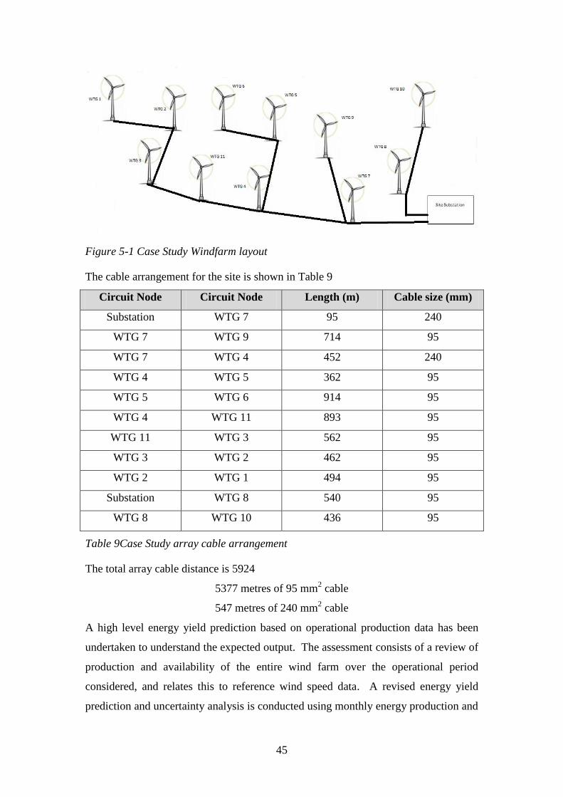
45
Figure 5-1 Case Study Windfarm layout
The cable arrangement for the site is shown in Table 9
Circuit Node Circuit Node Length (m) Cable size (mm)
Substation WTG 7 95 240
WTG 7 WTG 9 714 95
WTG 7 WTG 4 452 240
WTG 4 WTG 5 362 95
WTG 5 WTG 6 914 95
WTG 4 WTG 11 893 95
WTG 11 WTG 3 562 95
WTG 3 WTG 2 462 95
WTG 2 WTG 1 494 95
Substation WTG 8 540 95
WTG 8 WTG 10 436 95
Table 9Case Study array cable arrangement
The total array cable distance is 5924
5377 metres of 95 mm2 cable
547 metres of 240 mm2 cable
A high level energy yield prediction based on operational production data has been
undertaken to understand the expected output. The assessment consists of a review of
production and availability of the entire wind farm over the operational period
considered, and relates this to reference wind speed data. A revised energy yield
prediction and uncertainty analysis is conducted using monthly energy production and
46
reference wind speed data. This is delivered in the form of monthly operational
reports as described in 3.2.
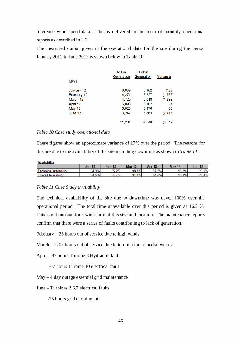
The measured output given in the operational data for the site during the period
January 2012 to June 2012 is shown below in Table 10
Table 10 Case study operational data
These figures show an approximate variance of 17% over the period. The reasons for
this are due to the availability of the site including downtime as shown in Table 11
Table 11 Case Study availability
The technical availability of the site due to downtime was never 100% over the
operational period. The total time unavailable over this period is given as 16.2 %.
This is not unusual for a wind farm of this size and location. The maintenance reports
confirm that there were a series of faults contributing to lack of generation.
February – 23 hours out of service due to high winds
March – 1207 hours out of service due to termination remedial works
April – 87 hours Turbine 8 Hydraulic fault
-67 hours Turbine 10 electrical fault
May – 4 day outage essential grid maintenance
June – Turbines 2,6,7 electrical faults
-75 hours grid curtailment

47
It can be derived that the generator has lost 17 % production over the period with 16
% of that due to availability issues. Approximately 0.5% of that is related to electrical
faults across the turbines. It may then be approximated that the expected electrical
losses for the plant over the period should be in the region of around 1.5 % of the
total.
It should be noted that some assumptions have been made due to the lack of actual
metered data and specific electrical losses per fault.
The site parameters were fed into the loss tool and the results witnessed in 5.2.
5.2. Results
Once all the parameters of the site were entered into the loss prediction tool the
following losses as shown in Error! Reference source not found.
Description Remarks Total Losses
(Watts) Percentage of Max Output
MV Collector Cables At estimated Operating Temperature 65,067 0.352%
2100KVA Export
Transformer Standard Losses 226,416 1.224%
LV Cables Ignore Losses 0 0.000%
Total 292,606 1.582%
Table 12 Case study loss calculation results
The loss calculation tool calculates the electrical losses to be 1.582 % which
according to the operational reports would be the expected losses from the electrical
components.

48
6. Conclusions
The main conclusion is that the tool performs to the level required by the electrical
department at SgurrEnergy. The calculations are within the correct order of
magnitude and the figures from the case study show that the tool calculates the losses
to a reasonable accuracy.
Some assumptions were made due to the lack of metered data but should not affect
the overall accuracy too much.
The tool should become more accurate with more datasets including inverters, WTG
transformers and transformers.
Metered data from the site would have conclusively proven the tools accuracy and it
is hoped that SgurrEnergy’s new O&M department will be able to supply this for
future projects.
The tool is not capable at the moment of replicating HV DC cable transmission losses
and as this is expected to be a growing market this omission should be rectified over
time.
The purpose of this thesis was to produce a tool that would provide accurate electrical
loss calculations for investors to be confidence with. The author concludes that this
has been achieved.

49
7. Further Work
If more time was available or further academic study was pursued, the following
topics could have been explored in relation to this body of work:
High Voltage Direct Current (HVDC) losses.
Expansion of the datasets to include less common cable and transformer
manufacturers
Dynamic ratings of cables to increase the current carrying capacity
Expansion of tool to model other renewable generation (Hydro, Wave)
50
8. References
Ackerman, T. (2012). Wind Power in Power Systems. Wiley.
Alasdair Miller, B. L. (2010). IFC Solar guidebook. Glasgow.
associates, S.-H. (n.d.). Total Machine control. Retrieved August 11, 2014, from Plant
or Manufacturing engineering: http://stewart-hay.com/plant1ie.htm
Colin Bayliss, B. H. (2007). Transmission and Distribution Electrical engineering.
Newnes.
Electronics, P. (2013). HEC-UL Solar inverter datasheet.
Heathcote, M. J. (2008). J&P Transformer Book. Newnes.
http://www.schneider-electric.com/downloads. (n.d.). Retrieved August 8, 2014, from
http://www.schneider-electric.com/: http://www.schneider-
electric.com/products/ww/en/3600-mv-transformers/3630-odt-oil-distribution-
transformers/60724-minera-ground-mounted/
Luo, F. L. (2013). Advanced DC/AC Inverters - Applications in Renewable Energy.
CRC Press.
Maximum HDMI Cable Length. (n.d.). Retrieved August 11, 2014, from
http://maximumhdmicablelengthtsrh.wordpress.com/
Moore, G. (1999). Electric Cables Handbook. Blackwell Science.
Papastergiou, K. (2010). Power Loss Calculations in Laarge Solar Parks.
Price, T. J. (2005). James Blyth - Britains First Modern Wind Power Engineer.
51
SgurrEnergy About. (n.d.). Retrieved August 20, 2014, from SgurrEnergy:
http://www.sgurrenergy.com/about-sgurr-energy/
SgurrEnergy Accreditations. (n.d.). Retrieved August 20, 2014, from SgurrEnergy:
http://www.sgurrenergy.com/about-sgurr-energy/accreditations/
SgurrEnergy Values. (n.d.). Retrieved August 20, 2014, from SgurrEnergy:
http://www.sgurrenergy.com/about-sgurr-energy/values/
Siddique, H. A. (2014). DC Collector Grid Configurations for Large Photovoltaic
Parks.
Weedy, B. M. (2004). Electric Power Systems. Chichester: Wiley.
Worzyk, T. (2009). Submarine Power Cables. Springer.
www.nexans.com/news. (n.d.). Retrieved August 08, 2014, from www.nexans.com:
http://www.nexans.com/eservice/Corporate-en/navigatepub_224833_-
23712/Nexans_wins_100_million_Euros_power_cable_contract.html
www.renewable energyworld.com. (n.d.). Retrieved 2014, from
http://www.renewableenergyworld.com/rea/news/article/2014/02/meet-the-
new-worlds-biggest-wind-turbine
www.whiteleewindfarm.co.uk/about. (n.d.).