a study of design improvements for a multi-tethered...
TRANSCRIPT

A Study of Design Improvements for a Multi-Tethered Aerostat System
François Deschênes
Department of Mechanical Engineering
McGill University
Montréal, Québec, Canada
March 2005
A thesis submitted to the Faculty of Graduate Studies and Research in partial
fulfillment of the requirements of the degree of
Masters of Engineering
© François Deschênes, 2005

ii
Abstract
The Large Adaptive Reflector is a Canadian design for a new radio telescope. The
receiver is held at the focus of the reflector by an aerostat tethered to the ground by
multiple tethers. One of the main goals in the design of this system is the minimization of
the motion of the receiver. Most perturbations are produced by the action of the wind on
the aerostat and transmitted to the confluence point via the leash that connects the aerostat
to the receiver. For that reason, this work focused on leash-related stabilization
techniques. Computer simulations were used to evaluate the benefits of different passive
and active methods. Among the passive approaches studied were the use of a constant
force spring and of a passive heave compensator. The active methods evaluated included
aerostat pitch control and active heave compensation. One of the more promising
approaches, a leash made of bungee cable, was evaluated experimentally on a prototype
of the system in Penticton, BC. Finally, a pitch control mechanism was designed. This
mechanism displaces the leash attachment point on the harness to pitch the aerostat nose
up or down.

iii
Résumé
Le LAR est un radiotélescope novateur conçu par un consortium canadien. Une des
principales composantes du LAR est un système de positionnement du récepteur
comprenant un ballon d’hélium retenu au sol à l’aide de câbles. Le but de ce système est
de positionner le récepteur au foyer du réflecteur et d’en minimiser le mouvement.
Comme la majeure partie des perturbations du système provient de l’action du vent sur
l’aérostat et que celles-ci sont transmises au récepteur à travers la laisse qui le relie à
l’aérostat, les techniques de stabilisation du récepteur étudiées dans la présente thèse sont
en lien avec la laisse. Afin d’évaluer les avantages des différentes techniques (passives et
actives) étudiées, une simulation numérique du système de positionnement fut utilisée.
L’utilisation d’un ressort à force constante ainsi que d’un compensateur passif de la laisse
font partie des méthodes passives étudiées tandis que le contrôle du lancement de
l’aérostat ainsi la compensation active de la laisse font partie des méthodes actives
étudiées. Une des méthodes les plus prometteuses, le remplacement de la laisse par un
câble élastique, fut évaluée expérimentalement sur un prototype situé à Penticton,
Colombie-Britannique. Finalement, un mécanisme permettant le déplacement du point
d’attache de la laisse sur le harnais dans le but de contrôler le lancement de l’aérostat fut
conçu.

iv
Table of Contents
Abstract.............................................................................................................................. ii
Résumé .............................................................................................................................. iii
Table of Contents ............................................................................................................. iv
List of Figures................................................................................................................... vi
List of Tables .................................................................................................................. viii
Acknowledgments ............................................................................................................ ix
Chapter 1 Introduction..................................................................................................... 1 1.1 Square Kilometre Array.......................................................................................1 1.2 Large Adaptive Reflector.....................................................................................2 1.3 Thesis Objective and Motivations .......................................................................4 1.4 Literature Survey .................................................................................................4
1.4.1 Single-Tethered Aerostats............................................................................5 1.4.2 Multi-Tethered Aerostats .............................................................................6 1.4.3 Heave Compensation ...................................................................................8
1.5 Thesis Organization .............................................................................................8
Chapter 2 Preliminary Study of Passive Methods ....................................................... 10 2.1. Introduction........................................................................................................10 2.2. System Configuration and Performance ............................................................10
2.2.1 Penticton Facility .......................................................................................11 2.2.2 Simulation ..................................................................................................12
2.3. Leash Properties.................................................................................................15 2.3.1 Leash Length..............................................................................................15 2.3.2 Leash Stiffness ...........................................................................................16 2.3.3 Leash Damping ..........................................................................................17
2.4. Constant Force Spring........................................................................................18 2.5. Passive Heave Compensation of the Leash .......................................................21
2.5.1 Pretension...................................................................................................23 2.6. Design Implications ...........................................................................................24
2.6.1 Reduction of the Leash Elasticity ..............................................................25 2.6.2 Passive Heave Compensation of the Leash ...............................................27
2.7. Comparison of the Passive Methods..................................................................30

v
Chapter 3 Preliminary Study of Active Alleviation Methods ..................................... 31 3.1 Introduction........................................................................................................31 3.2 Aerostat Pitch Control........................................................................................31
3.2.1 Aerostat Harness ........................................................................................32 3.2.2 Pitch Control ..............................................................................................34
3.3 Active Heave Compensation of the Leash.........................................................37 3.4 Design Implications ...........................................................................................40
3.4.1 Leash Attachment Point Actuation ............................................................40 3.4.2 Lateral Tailfin Actuation............................................................................41 3.4.3 Active Heave Compensation Actuation.....................................................43
3.5 Comparison of Active Methods .........................................................................43
Chapter 4 Detailed Study of the Bungee Leash............................................................ 45 4.1 Introduction........................................................................................................45 4.2 Bungee Leash Design ........................................................................................45
4.2.1 Choice of the Bungee Cable ......................................................................46 4.2.2 Design of the Bungee Leash Arrangement ................................................49 4.2.3 Bungee Leash Performance .......................................................................52
4.3 Test Set-Up and Procedure ................................................................................56 4.3.1 Test Setup...................................................................................................56 4.3.2 Procedure ...................................................................................................58
4.4 Results and Interpretation ..................................................................................61 4.4.1 Results........................................................................................................61 4.4.2 Interpretation..............................................................................................65
4.5 Conclusion .........................................................................................................69
Chapter 5 Design of a Variable Leash Attachment Point Mechanism ...................... 71 5.1 Introduction........................................................................................................71 5.2 Component Selection .........................................................................................72
5.2.1 Pulley .........................................................................................................72 5.2.2 Servo Motor ...............................................................................................73 5.2.3 Servo Amplifier .........................................................................................75 5.2.4 Gearing.......................................................................................................76
5.3 Mechanism Arrangement...................................................................................77 5.4 Performance .......................................................................................................79 5.5 Design Issues .....................................................................................................81
5.5.1 Mechanism Oscillation ..............................................................................81 5.5.2 Battery Power.............................................................................................82
5.6 Conclusion .........................................................................................................83
Chapter 6 Conclusion ..................................................................................................... 84 6.1 Recommendations for Future Work...................................................................87
References........................................................................................................................ 89

vi
List of Figures
Fig. 1.1. An artist’s conception of the LAR installation. ................................................ 2
Fig. 1.2. An actuated panel prototype in Penticton, BC.................................................. 3
Fig. 1.3. LAR’s receiver positioning system prototype in Penticton, BC....................... 7
Fig. 2.1. Penticton facility general scheme. .................................................................. 11
Fig. 2.2. Behaviour of the baseline system.................................................................... 14
Fig. 2.3. Payload errors of the baseline system with constant leash tension................. 15
Fig. 2.4. Confluence point position rms error as a function of leash length. ................ 16
Fig. 2.5. Confluence point position rms error as a function of leash stiffness. ............. 17
Fig. 2.6. Confluence point rms error as a function of leash damping ratio................... 18
Fig. 2.7. Uncoiling of a constant force spring............................................................... 19
Fig. 2.8. Baseline system with a 60-metre constant force spring.................................. 20
Fig. 2.9. Baseline system with a 10-metre constant force spring.................................. 21
Fig. 2.10. Location of a passive heave compensator in the system................................. 22
Fig. 2.11. Confluence point rms error and mean compensator length as a function of
passive alleviation stiffness............................................................................. 22
Fig. 2.12. Baseline system with a passive compensator.................................................. 24
Fig. 2.13. Representation of a passive heave compensation system. .............................. 28
Fig. 3.1. Penticton aerostat and harness. ....................................................................... 32
Fig. 3.2. Leash attachment point position with respect to the aerostat centre of
mass for a displacement of 1.4 metres on the harness. ................................... 33
Fig. 3.3. Aerostat pitch controlled using the leash attachment point position. ............. 34
Fig. 3.4. Aerostat pitch controlled using lateral tailfins deflection. .............................. 34
Fig. 3.5. Baseline system with pitch controller #2. ....................................................... 37
Fig. 3.6. Baseline system with leash speed control. ...................................................... 39
vii
Fig. 3.7. Leash attachment point actuation device. ....................................................... 41
Fig. 3.8. Penticton aerostat lateral fin............................................................................ 42
Fig. 3.9. Actuated lateral tailfin..................................................................................... 42
Fig. 4.1. Bungee stiffness characterization experimental setup. ................................... 47
Fig. 4.2. Example of elongation curve for a sheathed bungee cable............................. 47
Fig. 4.3. Load curve used to estimate the damping ratio of the BCI sample. ............... 49
Fig. 4.4. Custom-made bungee cord. ............................................................................ 51
Fig. 4.5. The three components of the bungee leash arrangement. ............................... 51
Fig. 4.6. Spectra leash and bungee leash configurations............................................... 52
Fig. 4.7. Payload motion for the Spectra and bungee leash configurations. ................. 53
Fig. 4.8. Payload rms error in function of aerostat net lift. ........................................... 54
Fig. 4.9. Payload motion for the baseline system with winch control. ......................... 56
Fig. 4.10. Instrument platform and ballonet platform. .................................................... 57
Fig. 4.11. Location of the instrument and ballonet platforms. ........................................ 58
Fig. 4.12. Penticton aerostat and trailer........................................................................... 59
Fig. 4.13. Two steps of the bungee leash releasing procedure........................................ 60
Fig. 4.14. Payload motion for the August 11th experiment. ............................................ 63
Fig. 4.15. Simulated payload motion with August 11th wind conditions. ....................... 64
Fig. 4.16. Simulation of Spectra Sample #10 with experimental top leash tension........ 67
Fig. 4.17. Simulation of bungee Sample #12 with experimental top leash tension. ....... 68
Fig. 4.18. Example of backup cable tangling (August 11th)............................................ 68
Fig. 5.1. Location of the leash attachment mechanism. ................................................ 72
Fig. 5.2. Pulley schemas and characteristics. ................................................................ 73
Fig. 5.3. Harness tension difference and speed for controller #2.................................. 74
Fig. 5.4. BSM80N-150 motor and characteristics......................................................... 75
Fig. 5.5. FDH2A05TR-EN23 amplifier and characteristics.......................................... 75
Fig. 5.6. Gear components and characteristics.............................................................. 77
Fig. 5.7. Leash Attachment Point Mechanism. ............................................................. 78
Fig. 5.8. Baseline system behaviour with the leash attachment mechanism................. 80
Fig. 5.9. Static equilibrium of the leash attachment mechanism................................... 81
Fig. 5.10. Mechanism oscillation for the simulation of Section 5.4. .............................. 82

viii
List of Tables
Table 2.1. Properties of some raw materials available as fibre........................................ 25
Table 2.2. Product EA of five Cortland Cable ropes....................................................... 26
Table 2.3. Comparison of the passive methods. .............................................................. 30
Table 3.1. Confluence point rms error produced by different pitch controllers. ............. 36
Table 3.2. Comparison of the active methods.................................................................. 44
Table 4.1. Properties of the BCI bungee sample.............................................................. 49
Table 4.2. Simulated Spectra and bungee leashes comparison........................................ 55
Table 4.3. Wind conditions sampling of August 11th experiment. .................................. 62
Table 4.4. Results in horizontal and vertical directions. .................................................. 65

ix
Acknowledgments
First and foremost, I would like to express my sincere gratitude to my advisor, Professor
Meyer Nahon. Although he probably does not suspect it, his determination has given me
the courage and motivation to persevere and to see my thesis to the end. I thank him for
his constant guidance, his dedication and his perspective, which has helped look at old
problems in new ways.
I would also like to acknowledge a number of McGill students with whom I worked on
the LAR project. I thank Casey Lambert for his advice and his help regarding the analysis
of the Penticton facility data, and I thank Gabriele Gilardi for helping me code the half-
bungee/half-Spectra leash in the LAR simulation. I thank Philippe Coulombe-Pontbriand
and Jennifer Pereira for their work on the integration of the wireless backup
communication system, and, Philippe, thank you for these incredible escapades at
MacDonald campus. My gratitude also goes out to Alexandre Boyer for waking me up at
the airport an hour before takeoff. Without his call, I would have missed a really nice
week in British Columbia.
Thanks to all the people at the Dominion Radio Astrophysical Observatory in Penticton,
especially Peter Dewdney, Donna Morgan and the aerostat “flight crew”: Dean Chalmers,
Richard Hellyer, Andrew Gray and Dave “Toffee” Del Rizzo. Dean, thank you for
introducing me to one of British Columbia’s greatest singers; and Richard, thanks for
shouting “RUN!” at the right moment. Quite possibly, you saved my life. I also cannot
forget Jean Bastien who installed the battery backup on the aerostat ballonet platform and
Angel Garcia who lodged me and drove me back and forth to the observatory every day
for a month.

x
Before working on the LAR, I had the chance to start a masters project in the Ambulatory
Robotics Laboratory, where I stayed even after my switch to the LAR project. I consider
this a chance since I met, in this lab, individuals who had a huge impact on my life and
radically changed my way of thinking. I thank James Andrew Smith, one of the finest
Francophiles I know, for all the conversations that allowed me to see my province from a
brand new perspective. I also thank Neil Neville for being my first McGill teammate.
This may seem insignificant today, but back then it meant a lot to me since I hardly spoke
English and I was a little scared. I also want to thank Christina Georgiades for
accompanying me through my thesis writing and job searching processes. Her moral
support was a lot more meaningful knowing that she was going through the same
obstacles. I thank Christopher Prahacs, the best opponent at Quake, for helping me design
the variable leash attachment point mechanism. I also express my sincere appreciation to
all the other great ARL people I had the chance to know: Don Campbell, Evgeni Kiriy,
Julien Marcil, Jacqui McCallum, Dave McMordie, Ioannis Poulakakis, Enrico Sabelli,
Akihiro Sato, Aaron Saunders, John “No Love” Sheldon, Matthew Smith, Charles
Steeves, Mike Tolley and Geneviève Vinois.
Outside the laboratory, I thank Philippe Cardou for his friendship and also for introducing
me to a lot of amazing people during these two years. I thank Geneviève Houde for all her
get-togethers, especially knowing that she would have preferred not to be the only one
who planned them. I thank them both, as well as Katia Bilodeau, Gabriel Meunier and
Guy Rouleau for the wonderful lunch times we shared at McGill.
Finally, thanks to Professor Clément Gosselin for arousing and feeding my interest in
robotics and to Professor Martin Buehler for giving me my first chance at McGill
University. Without your generosity and effort, none of this would be possible.
Funding for this research was provided by the Natural Sciences and Engineering Research
Council of Canada (NSERC). My personal funding was from le Fonds Québécois de la
Recherche sur la Nature et les Technologies (FQRNT).

xi
À mes parents et ma soeur Andrée-Anne.
Je vous adore!


1
Chapter 1
Introduction
1.1 Square Kilometre Array
Astronomers use radio telescopes (also named radio interferometers) to detect the
relatively long wavelength electromagnetic radiations emitted by outer space matter.
Since the first observations in 1932, radio astronomy has led, amongst others, to the
discovery of radio galaxies, quasars, pulsars and the cosmic microwave background.
According to the international radio astronomy community, the next step is the
observation of the formation of the early universe, including the emergence of the first
stars and galaxies. To achieve this, a revolutionary instrument, with an increase in
sensitivity of two orders of magnitude relative to existing interferometers, is needed
[1][2]. Since increasing a telescope’s sensitivity implies increasing its collecting area, this
instrument would need one square kilometre of collecting area – thirty times more than
the largest radio telescope ever built. This revolutionary instrument would be composed
of many antennas and is commonly known as the Square Kilometre Array (SKA) [3][4].
The project of designing the Square Kilometre Array has been undertaken by an
international consortium of radio astronomers and engineers representing more than
fifteen countries including Canada, USA, Europe, Australia, China, India and South
Africa. To keep the cost of such a large project reasonable, several international research
centres are presently developing completely new technologies. These include large arrays
of low-cost parabolic antennas, adaptive array technology and novel concepts for very
large, single-aperture antennas such as the LAR, which is the Canadian solution. The
timeline of the SKA project includes selection of the site in 2006 and of the final design
2
in 2008 for construction between 2012 and 2020. The expected cost of the SKA is one
billion US dollars.
1.2 Large Adaptive Reflector
Researchers at the National Research Council of Canada’s Herzberg Institute of
Astrophysics have suggested a novel design concept for the SKA known as the Large
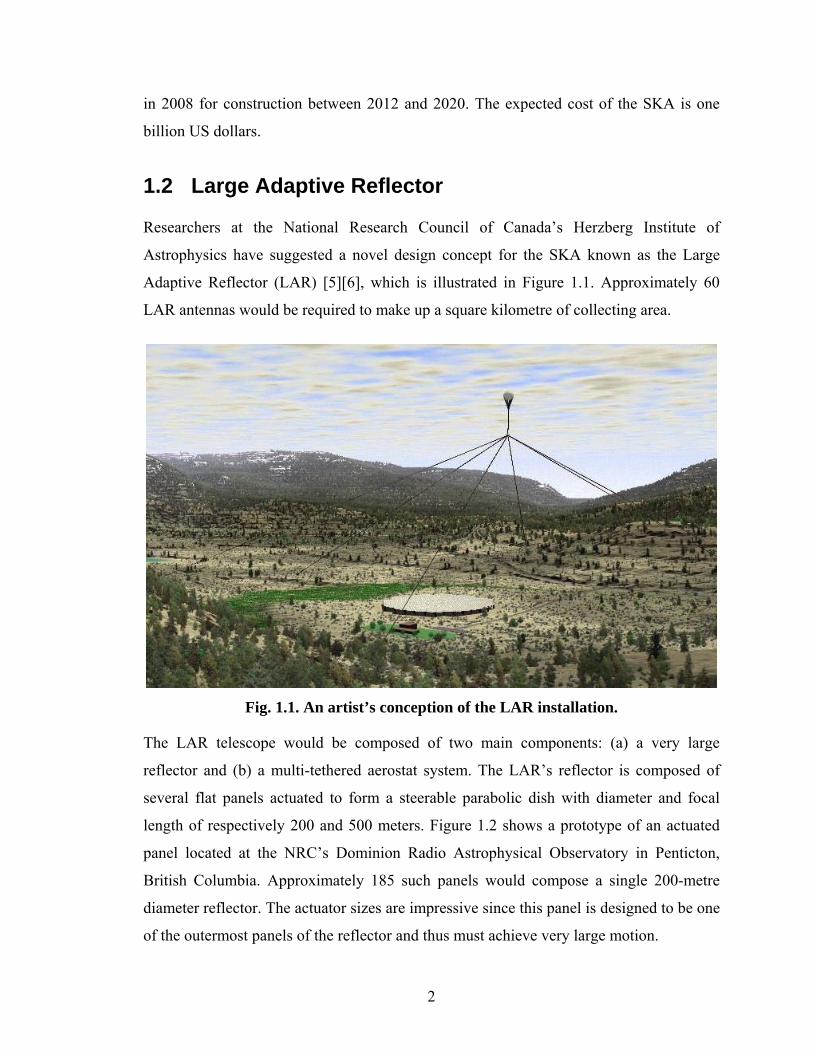
Adaptive Reflector (LAR) [5][6], which is illustrated in Figure 1.1. Approximately 60
LAR antennas would be required to make up a square kilometre of collecting area.
Fig. 1.1. An artist’s conception of the LAR installation.
The LAR telescope would be composed of two main components: (a) a very large
reflector and (b) a multi-tethered aerostat system. The LAR’s reflector is composed of
several flat panels actuated to form a steerable parabolic dish with diameter and focal
length of respectively 200 and 500 meters. Figure 1.2 shows a prototype of an actuated
panel located at the NRC’s Dominion Radio Astrophysical Observatory in Penticton,
British Columbia. Approximately 185 such panels would compose a single 200-metre
diameter reflector. The actuator sizes are impressive since this panel is designed to be one
of the outermost panels of the reflector and thus must achieve very large motion.

3
Fig. 1.2. An actuated panel prototype in Penticton, BC.
A multi-tethered aerostat system is used to hold the receiver package at the focal point of
the reflector, 500 metres aloft. This system is composed of a helium-filled aerostat
attached to the receiver package by a single tether commonly called the leash. The
receiver, also called focal package or payload, is fixed to the ground by three or more
tethers (see Figure 1.1). The LAR telescope is steered by modifying the reflector’s shape
and simultaneously varying the lengths of these tethers with winches located at the base
of each tether to position the receiver at the new focal point. For sufficient coverage of
the sky, the multi-tethered aerostat system must be able to position the focal package for a
range of zenith angles from 0 to 60o for all azimuths.
The Large Adaptive Reflector concept is a very promising approach for radio telescope
design. First, it permits the construction of larger fully steerable parabolic reflectors with
field-of-views comparable to those of much smaller antennas. Secondly, since it uses a
reflector with a large focal ratio (focal length divided by diameter), its off-axis
performance is exceptional. Finally, the relatively flat reflecting surface can be supported
on the ground in a distributed manner instead of being supported by a single mechanical
part as in the traditional designs, decreasing the cost per square metre of collecting area
by roughly an order of magnitude relative to conventional designs [5].

4
1.3 Thesis Objective and Motivations
The Large Adaptive Reflector concept looks very promising; however, its practical
feasibility raises some questions. One of the main uncertainties is whether or not the
multi-tethered aerostat system has the capacity to position the focal package to centimetre
accuracy, which is the precision required for good signal reception. The multi-tethered
tension structure is stiff enough to successfully resist wind forces and large enough to
filter out the highest frequency turbulence, but the present design is not good enough to
stabilize the receiver to centimetre accuracy.
In order to address the remaining payload disturbances, two active controllers will be
implemented in the LAR multi-tethered aerostat system. The first controller uses the
ground winches to vary the tether lengths and respond to the low frequency disturbances.
The second controller uses a parallel mechanism, mounted at the confluence point of the
tethers, to precisely stabilize the receiver at higher frequencies. It is estimated that this
five degrees of freedom parallel mechanism, which is called the Confluence Point
Mechanism (CPM), would be capable of correcting errors in a sphere of one metre and to
provide rotations of 0.5 rad about two axes.
However, the capacity of these two controllers to stabilize the receiver to centimetre
accuracy for all the configurations of the LAR multi-tethered aerostat system is far from
certain at this point as their design is not completed yet. In the eventuality that the winch
controller and the CPM are not sufficient, other stabilization techniques for the focal
package must be investigated. This is the focus of the present work, which is intended to
be preliminary. If they prove to be worthwhile, the stabilization techniques analysed here
will be further investigated and may be implemented in the LAR multi-tethered aerostat
system.
1.4 Literature Survey
This literature survey reviews the research performed on single-tethered and multi-
tethered aerostats. Additionally, work on heave compensation, which is a technique
commonly used in marine tethered systems, is presented. It is included since it is

5
envisioned that such a technique could be used in the LAR multi-tethered aerostat system
to decouple the aerostat and payload motions.
1.4.1 Single-Tethered Aerostats
Nearly all the literature on aerostats deals with streamlined aerostats. These consist of a
teardrop-shape ("streamlined") hull with 3 or 4 tailfins at the rear for stability, as shown
in Figure 1.3. The principal advantage of this shape relative to a spherical shape is that
they have lower drag and tend to have better survivability in high wind speeds. Single-
tethered aerostats have been the subject of many investigations, which can be separated
into linear and non-linear studies. DeLaurier performed the first study on the non-linear
dynamics of a single-tethered aerostat in 1972 [7]. His work consisted of a stability
analysis on a 2-D model for steady state wind conditions. DeLaurier added turbulence to
his analysis in 1977 [8]. Five years later, Jones and Krausman developed the first 3-D
non-linear dynamics model of a tethered aerostat, which included a lumped mass
discretized tether [9]. In 1983, Jones and DeLaurier enhanced this model by developing a
discretized aerostat modeling technique that took into account turbulence variation along
the length of the hull [10]. This work also estimated the aerodynamic properties of an
aerostat based on semi-empirical data. By linearizing the equations of motion developed
by Jones and DeLaurier, Badesha and Jones conducted a stability analysis of a large
commercial aerostat in 1993 [11]. Lambert and Nahon used another 3-D non-linear
dynamics model to perform a stability analysis of a single-tethered streamlined aerostat in
2003 [12]. In this work, the aerostat model was based on a component breakdown method
and the tether was discretized into lumped-mass nodes connected by lumped stiffness and
damping elements. It was found that the system remained stable for wind speeds up to
20 m/s and that the tether length had an effect on the stability.
Other works on single-tethered aerostats deal with experimental validation. In 1973, Redd
et al. presented a linear model of a tethered aerostat in a steady wind and validated it
using experimental data [13]. Even if this linear model neglected the coupling between
the tether and the aerostat, it highlighted that certain physical parameters of the system
had an important effect on its stability. Humphreys also used experimental data in 1997 to
validate his 3-D non-linear model of a towed, scaled aerostat [14]. Finally, in 2001, the

6
linearized dynamics model developed by Badesha and Jones [11] was validated by Jones
and Shroeder using real flight data provided by the US Army [15].
1.4.2 Multi-Tethered Aerostats
Little work has been done on multi-tethered aerostats other than on the LAR aerostat
system. The first researchers to demonstrate an interest in multi-tethered aerostats were
Leclaire and Rice in 1973 and Leclaire and Schumacher in 1974 [16][17]. These U.S. Air
Force researchers conducted an experimental study of tri-tethered aerostat systems. Their
experiments indicated that: (a) the payload of a tri-tethered system was much more stable
than the payload of an equivalent single-tethered system, and (b) separating the payload
and the aerostat by a leash reduced the payload motion further. In an attempt to capture
snapshot images of star surfaces, Le Coroller et al. designed and prototyped a
hypertelescope with focal optics suspended by a multi-tethered helium balloon
in 2004 [18]. The multi-tethered system consisted of two interconnected tether tripods,
one restraining the payload at an altitude of 35.6 metres and one restraining the leash
movement a few metres below the aerostat, which flew at an altitude of 140 metres. With
this system, they measured payload displacements of few millimetres for wind speeds up
to 3 m/s.
Research on the LAR multi-tethered aerostat system started in 1997. In 2000,
Fitzsimmons et al., of the National Research Council of Canada, presented a steady state
study of a tri-tethered aerostat system [19]. At the same time, Nahon assembled a
preliminary dynamics 3-D simulation of a multi-tethered spherical aerostat system
including a lumped mass tether model as well as winch control [20]. The encouraging
results of these studies regarding the precision of the multi-tethered aerostat as a
positioning system for the LAR led to a more detailed stage of analysis, which consisted
of simulation investigations together with experimental validations. In 2002, Nahon et al.
implemented a streamlined aerostat model in the computer simulation and performed a
comprehensive performance evaluation for different system configurations [21]. It was
found from that study that: (a) the system was mainly sensitive to the low frequency
turbulent gusts, (b) the spherical aerostat performed relatively better than the streamlined
aerostat in terms of receiver stabilization, and (c) for the worst-case receiver

7
configuration, which is 60o in zenith and azimuth, the receiver position error could be
kept under one metre if 50 kW were available at each winch.
Later, Lambert et al. used dimensional analysis to design a one-third-scale prototype of
the LAR positioning system [22][23]. The purpose of this prototype was to validate the
dynamics model used in the simulation and to evaluate the operational issues inherent to
multi-tethered aerostat systems. A streamlined aerostat was selected since it was thought
at that time that its relative low drag would be an important advantage for the positioning
system. However, this advantage came at the price of a fluctuating lift generated by wind
gusts on the aerostat hull [21]. The prototype was constructed on a National Research
Council site in Penticton, British Columbia, and is operational since the fall of 2002.
Figure 1.3 shows a picture of this tri-tethered streamlined aerostat prototype. In this
picture, we see the aerostat attached to the payload by the leash. The payload is attached
to the ground by four tethers: three of them resist the aerostat lift while the fourth one,
called the central tether (the darkest one in Figure 1.3), is slack and is used to power the
system. In 2005, Nahon et al. used experimental data provided by this prototype to
validate the simulation dynamics models, which proved to be remarkably accurate [24].
Fig. 1.3. LAR’s receiver positioning system prototype in Penticton, BC.

8
1.4.3 Heave Compensation
Heave compensation has been mainly investigated for use with remotely operated vehicle
(ROV) systems, which consist of a caged vehicle, a cable housing electrical and optical
conductors, and a support vessel. These unmanned systems are used for undersea
operations such as inspection and repair of marine structures and scientific exploration in
depths greater than two kilometres. In order to maximize the operating life of ROV
systems in rough seas, scientists have developed passive and active heave compensation
systems to decouple the motion of the cage from its support vessel. In 1988, Niedzwecki
and Thampi presented a study of a ship-mounted passive heave compensator [25].
Another analysis of a ship-mounted system was presented by Hover et al. in 1994 [26].
Both of these works highlighted that the cage motion could be exacerbated if the
compensator stiffness was poorly chosen. The first study of a cage-mounted passive
heave compensator was performed by Driscoll et al. in 2000 [27]. By including a lumped-
parameter heave compensation element into a ROV system computer simulation using a
lumped-mass tether model, it was found that the performance of ship-mounted and cage-
mounted pneumatic compensation systems in reducing the cage motion and the tether
tension was very similar. However, during extreme sea conditions, snap-loading of the
tether occurred with the ship-mounted system but not with the cage-mounted system. This
cage-mounted pneumatic compensation system was optimized numerically by Driscoll et
al. in 2001 [28]. Eide enhanced this 1-D computer simulation of a ROV system by
implementing an irregular wave model as well as a ship-mounted active heave
compensator in 2003 [29]. This enhanced simulation was used to compare three types of
controller: PID, LQG and H∞; for an active heave compensator. For most of the cases
investigated, the performance of the LQG and H∞ controllers was better than that of the
PID controller, for which gain tuning was very time consuming. Furthermore, the
performance of the LQG controller proved to be more consistent than the others in
minimizing the cage motion, tether tension fluctuations and required compensator power.
1.5 Thesis Organization
The focus of the present work is the investigation of methods for stabilizing the receiver
of the LAR multi-tethered aerostat system other than winch control and CPM control.

9
In Chapter 2, a preliminary study of passive design improvements for the LAR multi-
tethered aerostat system is performed. The Penticton experimental one-third-scale facility
is first presented [23]. A dynamic simulation of a multi-tethered aerostat system
developed by Nahon et al. [20][21] is then used to assess the capacity of several passive
methods to reduce the receiver motion. These different methods are (a) the modification
of the leash properties, (b) the use of a constant force spring, and (c) passive heave
compensation. They are applied to the same simulated baseline multi-tethered system in
order to compare them with respect to their payload rms motion. Finally, these passive
methods are evaluated in terms of their design implications.
In Chapter 3, an analysis similar to the one of Chapter 2 is applied to three active
methods: (a) aerostat pitch control using harness shape modification, (b) aerostat pitch
control using tailfin deflection, and (c) active heave compensation. They are first
simulated in the baseline system to assess their capacity to reduce the receiver motion and
then their design implications are evaluated.
In Chapter 4, a detailed design of a bungee leash is performed and implemented in the
Penticton facility for testing. The bungee leash arrangement is first designed and then, the
Penticton test set-up as well as the launching and retrieving procedures are explained.
Finally, the results of the experiments are presented and interpreted, followed by a
discussion of the bungee leash approach.
A detailed design of a leash attachment point mechanism is provided in Chapter 5. This
mechanism is used to displace the leash attachment point on the harness in order to pitch
the aerostat nose up or down. The different components of the mechanism are first
selected. Then, the mechanism arrangement is presented and implemented in the
simulated baseline system. The simulation results are then interpreted and design
improvements are discussed.
Chapter 6 provides the conclusions of this research as well as recommendations for future
work.

10
Chapter 2
Preliminary Study of Passive Methods
2.1. Introduction
In this chapter, a preliminary study of passive methods is performed in order to identify
techniques that improve the multi-tethered aerostat system performance. By passive, we
mean any device that is not actively controlled. In Section 2.2, we present the Penticton
experimental facility and the simulation we use in our study. We also show in that section
that more than 90% of the payload perturbations come from the aerostat. Consequently,
the three passive approaches studied in this chapter address methods to reduce
transmission of these perturbations. These methods are:
- Modification of the leash properties (Section 2.3)
- Use of a constant force spring (Section 2.4)
- Passive heave compensation (Section 2.5)
In Section 2.6, we investigate the design implications of two of the passive methods, and
finally, a summary of Chapter 2 is presented in Section 2.7.
2.2. System Configuration and Performance
In this section, the tools used to compare the different passive methods discussed in this
chapter are presented. We focus our study on the multi-tethered aerostat system located in
Penticton, British Columbia, since it will allow us to perform experimental validation, as

11
needed. We first present the configuration of this system and then discuss the simulation
used to perform the study.
2.2.1 Penticton Facility
A one-third-scale tri-tethered aerostat system is presently being tested in Penticton as a
proof of concept for the LAR radio telescope proposal. As mentioned in Section 1.2, the
LAR multi-tethered aerostat system is used as a positioning device for the receiver
package. The purpose of the Penticton prototype is to validate the dynamics model used
in the simulation developed by Nahon et al. [20][21], to demonstrate the accuracy of the
positioning system and to evaluate the operational issues inherent to multi-tethered
aerostat systems. This multi-tethered aerostat prototype is composed of three tethers,
three winches, a payload, a leash and a streamlined aerostat (see Figure 2.1).
Fig. 2.1. Penticton facility general scheme.
Instruments are mounted at the payload and at the aerostat to measure the system states
during flight. Among others, these instruments comprise GPS receivers, load cells, a wind
sensor and an inertial measurement unit. These instruments are powered from the ground
through the central tether, a fourth tether connected to the payload, as well as through the
leash for the aerostat instruments. Data from all sensors are transmitted to a ground
computer by two radio modems and via a RS-485 link that pass through the central tether
and the leash.

12
The winches are located at the base of the tethers in order to actively control their lengths.
These winches receive their command signals from the ground computer through a fibre
optic network. In the multi-tethered aerostat positioning system, the ground winches are
used in two different ways: (a) to steer the payload to a new location and (b) to
compensate for payload disturbances.
Between experiments, the aerostat is stored in a hangar. When an experiment is to be
performed, the aerostat is moved with a trailer to the launch location. The system is
launched and retrieved using a main winch located on the trailer, on which are initially
spooled the central tether and the leash.
The Penticton facility has a winch radius of 400 metres, a focal length of about
170 metres as well as a leash of 200 metres. The tethers are made of Plasma material
while the leash is made of Spectra [30]. All have a diameter of 6 mm. In this chapter, we
evaluate the performance of different passive methods by simulating this same system.
2.2.2 Simulation
The dynamics simulation developed by Nahon et al. [20][21] uses a mathematical model
of the tethered aerostat system that has been widely discussed elsewhere, but we will
briefly review its main features.
The aerodynamic forces acting on the streamlined aerostat components (hull and fins) are
first calculated separately and then summed to provide the aerostat overall behaviour as
well as the magnitude and direction of the force acting at the top of the leash [21]. Each
cable is modeled using a lumped-mass model [12], meaning that each continuous tether is
discretized into lumps joined by massless segments. The payload joins all the cables
together and is modeled as a 0.8-m (the diameter of the instrument platform) sphere
whose drag coefficient varies with Reynolds number [21]. The internal forces (stiffness
and damping) as well as the external forces (aerodynamics and weight) are used to
formulate the equations of motion for each lumped mass. The only input to the system is
a wind that varies with altitude as a function of Earth’s boundary layer to which is added
turbulent gusts following a von Karman spectrum [21]. A fourth-order Runge-Kutta

13
numerical integration routine is used to solve the resulting system of nonlinear dynamic
equations [31].
To be consistent in our analysis, we choose a special case where the system configuration
and the wind conditions are fixed. We call this case the baseline system. For the baseline
system, the aerostat net lift is chosen to be 2.7 kN, which is the maximum net lift
measured in Penticton. Furthermore, the payload is positioned at zero degree in zenith
and azimuth, meaning that all three tethers have the same length, which is 435 metres.
The mean wind comes from the North and is constant at 5 m/s. Turbulence is included
and no winch control is used. For each simulation, values different from the baseline
parameters will be specified.
The simulation is divided in two main parts: static and dynamic analysis. The initial state
of the system is first calculated by the static analysis and is then used as a starting point
by the dynamic analysis to compute the system state at each time step. For the baseline
system, the simulation yields the time histories shown in Figure 2.2, where the payload
and aerostat errors are calculated with respect to their mean values. The aerostat rotations
are calculated with respect to their mean values.
In this chapter, we evaluate the different passive methods by comparing their capacity to
stabilize the payload. The Root Mean Square (RMS) of their confluence point position
error ∆(t) is used:
[ ]∫ ∆=∆T
RMS dttT 0
2)(1 (2.1)
where t is the time and T the total simulated time interval.
The confluence point position rms error of the baseline system is 19 cm. This is the value
that we aim to reduce throughout this chapter. Using the simulation, we found that
replacing the aerostat by a constant force equal in magnitude and direction to the baseline
system mean leash tension produces a payload rms error of 0.5 cm. We therefore focus
our analysis on the perturbations produced by the aerostat and transmitted through the
leash.

14
Fig. 2.2. Behaviour of the baseline system.
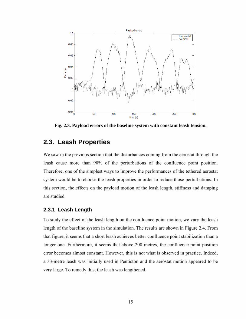
Since it is unlikely that we could stabilize the aerostat motion sufficiently to get a steady
leash orientation, stabilizing the leash tension magnitude is our main objective. If the
magnitude of the leash tension was constant but its direction fluctuated as in the baseline
case, we would get the system behaviour shown in Figure 2.3. In that figure, the top leash
tension is equal to the baseline mean leash tension, and the payload rms motion decreases
from 19 cm to 5 cm, a reduction of approximately 75% that is still highly desirable. By
comparing Figures 2.3 and 2.2 we deduce that variation in the leash tension magnitude
leads to fluctuations in vertical payload motion while variation in its direction leads to
fluctuations in horizontal payload motion.
15
Fig. 2.3. Payload errors of the baseline system with constant leash tension.
2.3. Leash Properties
We saw in the previous section that the disturbances coming from the aerostat through the
leash cause more than 90% of the perturbations of the confluence point position.
Therefore, one of the simplest ways to improve the performances of the tethered aerostat
system would be to choose the leash properties in order to reduce those perturbations. In
this section, the effects on the payload motion of the leash length, stiffness and damping
are studied.
2.3.1 Leash Length
To study the effect of the leash length on the confluence point motion, we vary the leash
length of the baseline system in the simulation. The results are shown in Figure 2.4. From
that figure, it seems that a short leash achieves better confluence point stabilization than a
longer one. Furthermore, it seems that above 200 metres, the confluence point position
error becomes almost constant. However, this is not what is observed in practice. Indeed,
a 33-metre leash was initially used in Penticton and the aerostat motion appeared to be
very large. To remedy this, the leash was lengthened.

16
0
0.05
0.1
0.15
0.2
0.25
0 50 100 150 200 250 300
Leash length (m)
Con
fluen
ce p
oint
RM
S er
ror (
m)
Baseline System
Fig. 2.4. Confluence point position rms error as a function of leash length.
On the other hand, we do not have quantitative results to confirm those observations. It is
possible that the perceived behaviour does not truly reflect larger or smaller confluence
point motion. For example, an operator tends to observe (and interpret) the frequency and
amplitude of oscillation of the aerostat motion. However, confluence point errors are
caused primarily by variation in the leash force. It is not clear that the correspondence
between these is direct. In order to better understand these issues quantitatively, a small-
scale facility is being constructed at McGill to provide more detailed data.
It is clear from the operational standpoint that installing a short leash would not be
beneficial. Additionally, the potential performance improvements (Figure 2.4) are not
very large. Shortening the leash length is therefore dropped from further consideration in
this study.
2.3.2 Leash Stiffness
In this subsection, we study the effect of the leash stiffness on the confluence point
motion. The stiffness of the leash is related to three parameters: its section area (A), its
unstretched length (lu) and its Young’s modulus (E) according to ulEAk = . To study the
effect of leash stiffness, we vary its Young’s modulus from 7.07x10⁵ to 7.07x10¹⁰ Pa in
17
the simulation, while keeping its unstretched length and its diameter constant. As a result,
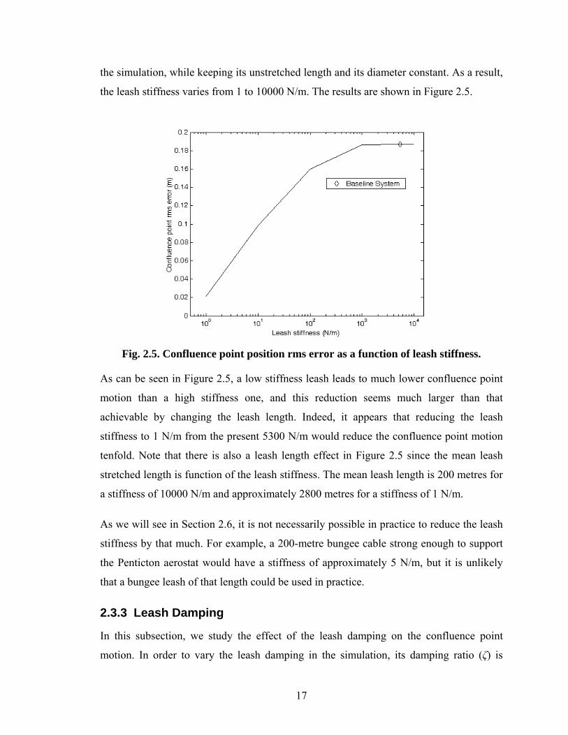
the leash stiffness varies from 1 to 10000 N/m. The results are shown in Figure 2.5.
Fig. 2.5. Confluence point position rms error as a function of leash stiffness.
As can be seen in Figure 2.5, a low stiffness leash leads to much lower confluence point
motion than a high stiffness one, and this reduction seems much larger than that
achievable by changing the leash length. Indeed, it appears that reducing the leash
stiffness to 1 N/m from the present 5300 N/m would reduce the confluence point motion
tenfold. Note that there is also a leash length effect in Figure 2.5 since the mean leash
stretched length is function of the leash stiffness. The mean leash length is 200 metres for
a stiffness of 10000 N/m and approximately 2800 metres for a stiffness of 1 N/m.
As we will see in Section 2.6, it is not necessarily possible in practice to reduce the leash
stiffness by that much. For example, a 200-metre bungee cable strong enough to support
the Penticton aerostat would have a stiffness of approximately 5 N/m, but it is unlikely
that a bungee leash of that length could be used in practice.
2.3.3 Leash Damping
In this subsection, we study the effect of the leash damping on the confluence point
motion. In order to vary the leash damping in the simulation, its damping ratio (ζ) is
18
varied from zero to one. The damping ratio is defined as crC
C=ζ where C is the actual
damping coefficient and Ccr is the critical damping coefficient. In our case, the critical
damping coefficient of each leash element is calculated at the first time step as
gkT
C ecr
⋅= 2 , where Te is the element tension, k the element stiffness and g the
gravitational acceleration. The results are shown in Figure 2.6.
0.17
0.175
0.18
0.185
0.19
0.195
0.2
0 0.2 0.4 0.6 0.8 1
Leash damping ratio
Con
fluen
ce p
oint
RM
S er
ror (
m) Baseline System
Fig. 2.6. Confluence point rms error as a function of leash damping ratio.
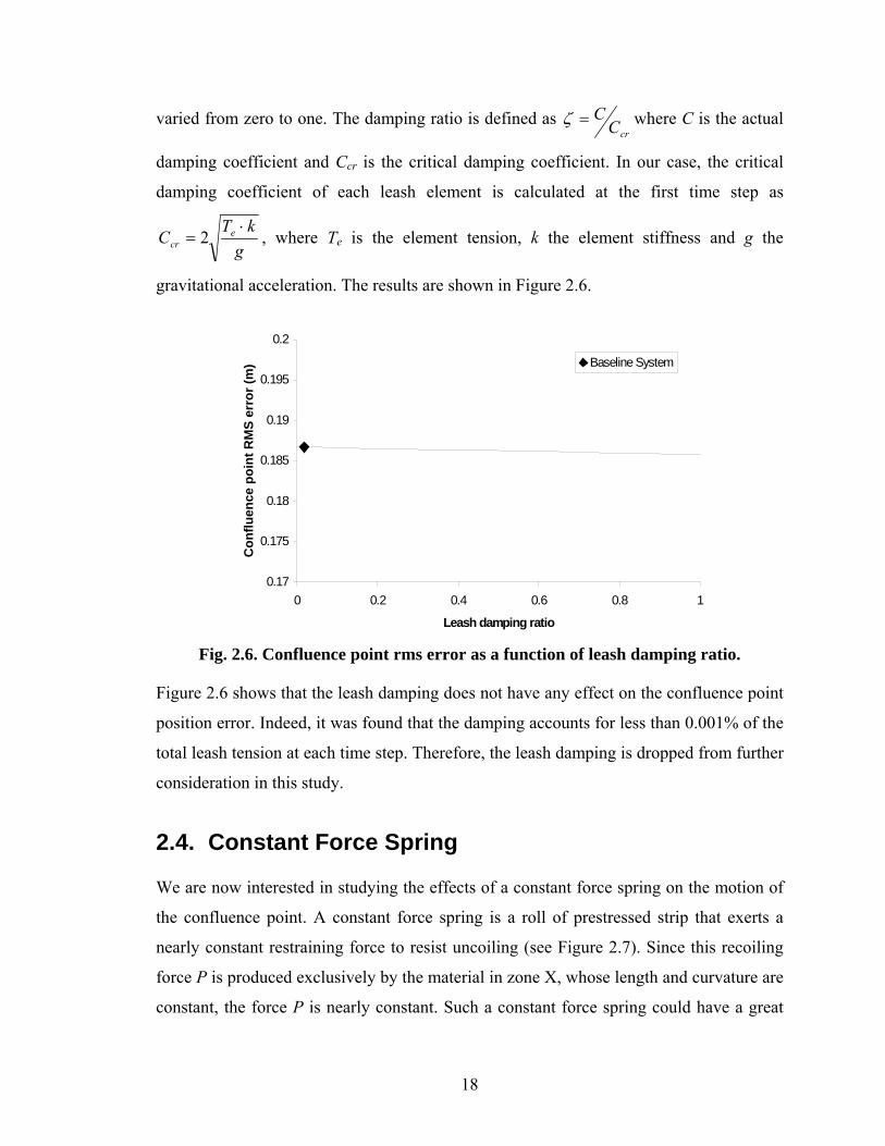
Figure 2.6 shows that the leash damping does not have any effect on the confluence point
position error. Indeed, it was found that the damping accounts for less than 0.001% of the
total leash tension at each time step. Therefore, the leash damping is dropped from further
consideration in this study.
2.4. Constant Force Spring
We are now interested in studying the effects of a constant force spring on the motion of
the confluence point. A constant force spring is a roll of prestressed strip that exerts a
nearly constant restraining force to resist uncoiling (see Figure 2.7). Since this recoiling
force P is produced exclusively by the material in zone X, whose length and curvature are
constant, the force P is nearly constant. Such a constant force spring could have a great

19
influence on the confluence point position error, as it would completely cancel the leash
tension disturbances. However, the largest commonly available constant force springs
only have a force of 180 N and the longest found is two metres long. Nevertheless, in this
section, we investigate the potential benefits of such a device assuming it was available.
Fig. 2.7. Uncoiling of a constant force spring [32].
The constant force spring is included in the simulation dynamics analysis with a constant
force equal to the leash initial tension. Indeed, including the spring in the static analysis
with a force different from the leash initial tension produces instability in the simulation.
The device is incorporated in the existing finite-element lumped-mass model as a single
lumped-parameter element at the bottom of the leash. Furthermore, the constant force
spring has a finite length. When one of its limits is reached, the spring becomes
ineffective.
The results of two simulations are presented in Figures 2.8 and 2.9 to demonstrate the
effects of the constant force spring: the first for a spring with a total travel of
60 metres (±30m) and the second for a spring with a travel of ten metres (±5m). In both
cases, the initial leash tension computed in the static analysis is approximately 2.6 kN.
As can be seen in Figure 2.8, the 60-metre spring is long enough for the wind conditions,
and its travel limits are never reached. With such a spring, the leash tension is constant for
the whole simulation and the rms motion of the confluence point is 5.4 cm instead of
19 cm for the baseline case (≈ 28%).
The results degrade significantly when the constant force spring is too short. Indeed,
when the constant force spring hits one of its stops, a discontinuity occurs in the leash
tension and the confluence point position error rises sharply. In the case of the 10-metre
spring (see Figure 2.9), the rms motion of the confluence point is only reduced to 15 cm.

20
Fig. 2.8. Baseline system with a 60-metre constant force spring.
It was mentioned in Section 2.2 that a system with constant leash tension and direction
would have its confluence point motion reduced to 4% of the baseline case. The constant
force spring reduces the motion “only” to 30% of the baseline case because it only
renders the magnitude of the leash tension constant — the direction still fluctuates.
The results of this section emphasize two points: (a) the constant force spring should be
long enough not to hit its stops too frequently, and (b) the spring force must be very close
to the mean leash tension or the travel required becomes very large. Since that mean
tension is a function of the wind conditions, which fluctuate, some other means would
have to be used to maintain a constant mean leash tension. Chapter 3 discusses possible
approaches for doing this. However, since this would entail too much complexity and it is
very unlikely that a suitably sized constant force device could be fabricated, this approach
is not considered further.

21
Fig. 2.9. Baseline system with a 10-metre constant force spring.
2.5. Passive Heave Compensation of the Leash
A passive heave compensator is a passive mechanism that includes a spring and a damper
that could be installed between the leash and the payload (see Figure 2.10) in order to
decouple the payload and aerostat motions. One advantage of such a compensator is that
arbitrary properties could be selected without being limited by rope materials.
In the simulation, passive heave compensation is included in the existing finite-element
lumped-mass model as a single lumped-parameter element, at the bottom of the leash.
The simulation is used to study the effect of the passive compensation stiffness on the
motion of the confluence point. Figure 2.11 shows (a) the rms error of the confluence
point position as well as (b) the mean value of the compensator length as functions of the
compensator stiffness.
As can be seen in Figure 2.11a, it is possible in principle to obtain very small confluence
point position error with a passive alleviation stiffness of 1 N/m, which is consistent with
the previous results for variations of the leash stiffness (Figure 2.5). Figure 2.11b shows
that the mean length of a passive alleviation system with a stiffness of 1 N/m is more than
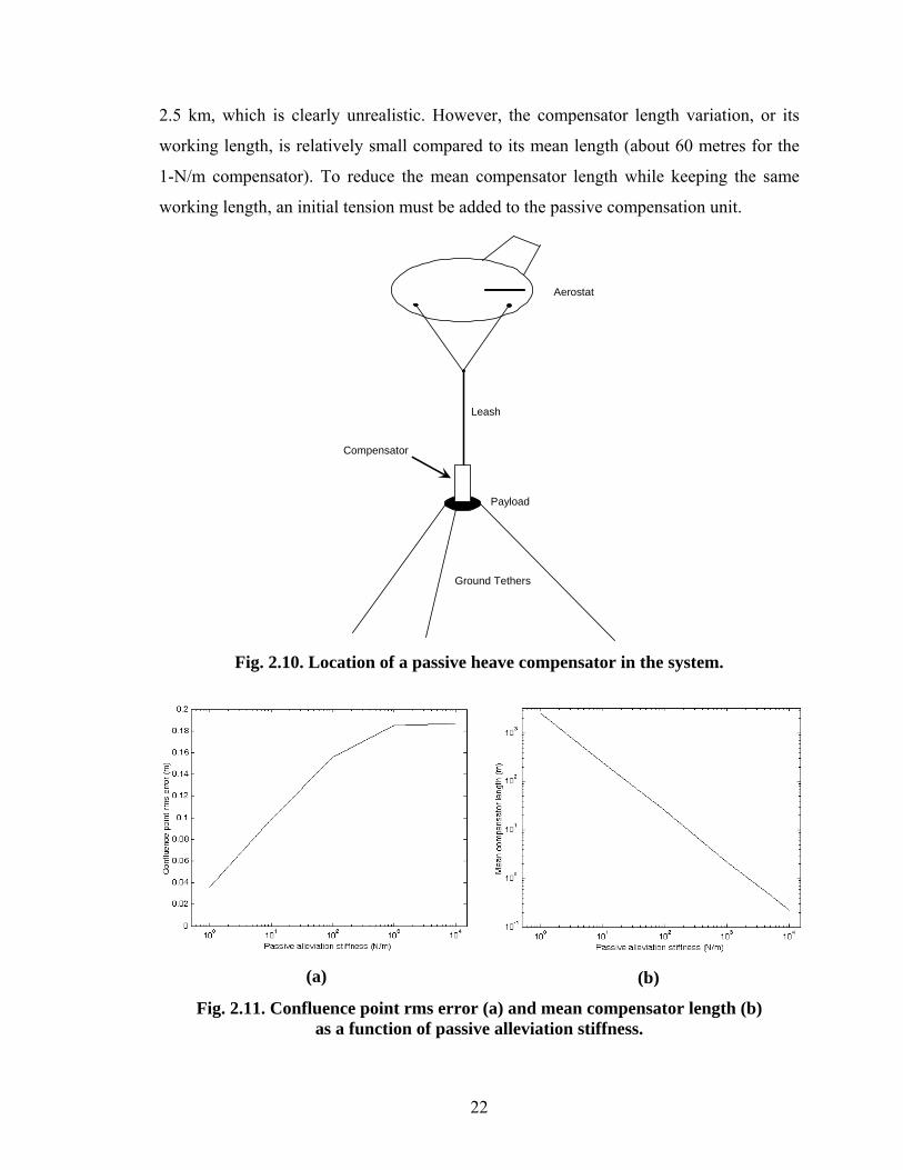
22
2.5 km, which is clearly unrealistic. However, the compensator length variation, or its
working length, is relatively small compared to its mean length (about 60 metres for the
1-N/m compensator). To reduce the mean compensator length while keeping the same
working length, an initial tension must be added to the passive compensation unit.
Payload
Aerostat
Ground Tethers
Leash
Compensator
Fig. 2.10. Location of a passive heave compensator in the system.
(a) (b)
Fig. 2.11. Confluence point rms error (a) and mean compensator length (b) as a function of passive alleviation stiffness.

23
2.5.1 Pretension
A pretension has to be added to a passive compensator in order to make it usable in
practice. Such a pretension would be added to the compensator spring in order to avoid
the excessive mean length needed otherwise.
In this subsection, the effects of adding initial tension to the passive alleviation element
are studied. In the simulation, the pretension (Tpre) is added to the elastic tension (kδ) of
the leash bottom element to give the total passive compensator tension (Tp):
prep TkT += δ (2.2)
For this study, the passive compensator stiffness is kept at 1 N/m since it is for this
stiffness that the best results were previously achieved. In selecting an appropriate value
of the pretension, it was found that, as pretension increased, the error of the confluence
point tended to increase. Theoretically, this should not have been the case. Indeed, adding
pretension to the passive compensator should affect only its mean length. Upon further
investigation, it was found that this was due to the effect of the pretension on the aerostat
altitude. Indeed, the wind forces, the turbulence and the air density are all functions of
altitude. Thus, by modifying the pretension, the altitude of the aerostat and the forces
acting on the system vary.
We found that a compensator with pretension and stiffness equal to 2.6 kN and 1 N/m
would reduce the confluence point position rms error to 4 cm and would require a
working length of about 60 metres (see Figure 2.12).

24
Fig. 2.12. Baseline system with a passive compensator.
By comparing Figures 2.8 and 2.12, we note that the passive heave compensator with a
stiffness of 1 N/m has the same effect as the constant force spring. Consequently, the
comments related to constant force springs at the end of Section 2.4 are also applicable to
passive compensators: (a) the working length of a passive alleviation device should be
long enough and (b) the pretension should be kept slightly below the minimum leash
tension or the compensator will hit one of its stops; this can be done either by controlling
the pretension or the leash tension. Chapter 3 presents some techniques to actively
stabilize the leash tension. We will discuss the design implications of building a passive
heave compensator with pretension in Subsection 2.6.2.
2.6. Design Implications
Until now, our analysis has mainly concentrated on the reduction of confluence point
motion to evaluate the performance of each passive method. However, the feasibility of
implementation of each approach is also very important. In this section, we perform a
preliminary evaluation of the design implications of two passive methods: reducing the
leash elasticity and passive heave compensation. Only those two are considered since the
25
other approaches did not improve the performance significantly enough or were judged to
be impractical.
2.6.1 Reduction of the Leash Elasticity
The results of Section 2.3 indicated that a substantial improvement in system performance
could be obtained by reducing the leash stiffness. With this in mind, we first consider the
properties of different raw materials used to construct braided ropes. Table 2.1 shows a
selection of materials available as fibre:
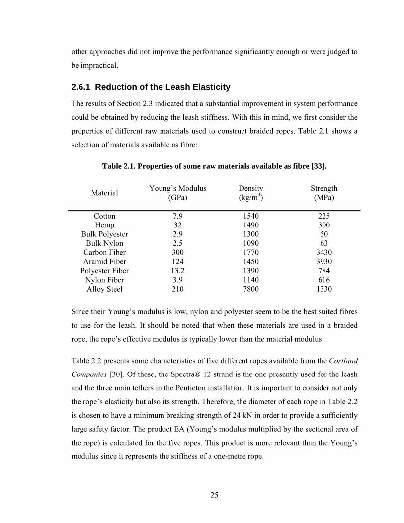
Table 2.1. Properties of some raw materials available as fibre [33].
Material Young’s Modulus (GPa)
Density (kg/m3)
Strength (MPa)
Cotton 7.9 1540 225 Hemp 32 1490 300
Bulk Polyester 2.9 1300 50 Bulk Nylon 2.5 1090 63
Carbon Fiber 300 1770 3430 Aramid Fiber 124 1450 3930
Polyester Fiber 13.2 1390 784 Nylon Fiber 3.9 1140 616 Alloy Steel 210 7800 1330
Since their Young’s modulus is low, nylon and polyester seem to be the best suited fibres
to use for the leash. It should be noted that when these materials are used in a braided
rope, the rope’s effective modulus is typically lower than the material modulus.
Table 2.2 presents some characteristics of five different ropes available from the Cortland
Companies [30]. Of these, the Spectra® 12 strand is the one presently used for the leash
and the three main tethers in the Penticton installation. It is important to consider not only
the rope’s elasticity but also its strength. Therefore, the diameter of each rope in Table 2.2
is chosen to have a minimum breaking strength of 24 kN in order to provide a sufficiently
large safety factor. The product EA (Young’s modulus multiplied by the sectional area of
the rope) is calculated for the five ropes. This product is more relevant than the Young’s
modulus since it represents the stiffness of a one-metre rope.
26
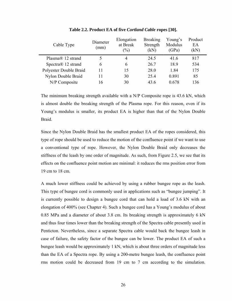
Table 2.2. Product EA of five Cortland Cable ropes [30].
Cable Type Diameter (mm)
Elongation at Break
(%)
Breaking Strength
(kN)
Young’s Modulus
(GPa)
Product EA
(kN)
Plasma® 12 strand 5 4 24.5 41.6 817 Spectra® 12 strand 6 6 26.7 18.9 534
Polyester Double Braid 11 15 28.0 1.84 175 Nylon Double Braid 11 30 25.4 0.891 85
N/P Composite 16 30 43.6 0.678 136
The minimum breaking strength available with a N/P Composite rope is 43.6 kN, which
is almost double the breaking strength of the Plasma rope. For this reason, even if its
Young’s modulus is smaller, its product EA is higher than that of the Nylon Double
Braid.
Since the Nylon Double Braid has the smallest product EA of the ropes considered, this
type of rope should be used to reduce the motion of the confluence point if we want to use
a conventional type of rope. However, the Nylon Double Braid only decreases the
stiffness of the leash by one order of magnitude. As such, from Figure 2.5, we see that its
effects on the confluence point motion are minimal: it reduces the rms position error from
19 cm to 18 cm.
A much lower stiffness could be achieved by using a rubber bungee rope as the leash.
This type of bungee cord is commonly used in applications such as “bungee jumping”. It
is currently possible to design a bungee cord that can hold a load of 3.6 kN with an
elongation of 400% (see Chapter 4). Such a bungee cord has a Young’s modulus of about
0.85 MPa and a diameter of about 3.8 cm. Its breaking strength is approximately 6 kN
and thus four times lower than the breaking strength of the Spectra cable presently used in
Penticton. Nevertheless, since a separate Spectra cable would back the bungee leash in
case of failure, the safety factor of the bungee can be lower. The product EA of such a
bungee leash would be approximately 1 kN, which is about three orders of magnitude less
than the EA of a Spectra rope. By using a 200-metre bungee leash, the confluence point
rms motion could be decreased from 19 cm to 7 cm according to the simulation.

27
However, we will see in Chapter 4 that because it can stretch to 400%, there is a practical
limit to the length of a bungee leash.
There are some drawbacks associated with a bungee leash. First, it would be much
heavier than a conventional rope. Secondly, a tether parallel to the bungee leash would
have to be installed for two reasons: (a) as explained in the previous paragraph, a safety
cable is needed since the safety factor of a bungee rope would be too low and (b) the
electrical wires that connect the aerostat to the ground need the protection of a stiff rope
or they will break. Other operational constraints arising from the use of the bungee leash
will be discussed in Chapter 4.
2.6.2 Passive Heave Compensation of the Leash
A passive heave compensation system for an underwater remotely operated vehicle
system was discussed in [27]. In that application, the mean tension was also very large
relative to the tension variations. As can be seen in Figure 2.13, the proposed design uses
a pneumatic spring and an accumulator to control respectively the stiffness and the
pretension of the compensator. A system of pulleys is included to increase the working
length of the compensator.
The passive compensation system presented in [27] appears well suited to our application
since (a) the operational problems it addresses are very similar to ours and (b) the
pneumatic solution it proposes would be relatively lightweight. In order to determine the
complexity that such a passive alleviation would add to the system, we adapt this
compensator design to our application.
First, to obtain a reasonably compact system we assume that the pneumatic piston would
have a length of 0.5 metre and a stiffness of 1 N/m, the stiffness that resulted in the lowest
confluence point rms motion in the previous section. According to the simulations done in
Section 2.5, such a passive heave compensator would need a travel of approximately 64
metres. Therefore, a system of seven pulley loops would be needed to get that working
length from a 0.5-metre piston ( 5.0264
7 = ). This system of pulleys would add weight and
complexity to the passive compensator.

28
Fig. 2.13. Representation of a passive heave compensation system [27].
According to [27], the volume of the accumulator can be found from:
111
1
−⎟⎟⎠
⎞⎜⎜⎝
⎛−+
= nTp
R
ppa
AV
δ (2.3)
where p represents the amplitude of the tension perturbations as a fraction of the mean
load, Ap is the piston section, a is the number of pulley loops, δT is the working length and
n is the ratio of specific heats of the gas which is 1.4 for air. We have already determined
that 7=a and 64=Tδ metres. Once again to obtain a reasonably compact system, we
assume a compensator piston diameter of 15 cm, which would have an area of
approximately 0.002 m2. To assess the value of p, we simulate the system with the
passive compensator of Subsection 2.5.1 and find that the minimum, the mean and the
maximum leash tension values are respectively 2553 N, 2573 N and 2610 N.
Therefore,
015.02753
25532753,2753
27532610max ≅⎟⎠⎞
⎜⎝⎛ −−
=p
and using Equation 2.3 we find an accumulator volume of 0.02 m3.

29
This means that the accumulator could be a cylinder of 20 cm diameter with a stroke of
65 cm. The maximum pressure inside the accumulator would be
2.9002.026107max
max =⋅
==pA
aTP MPa
The values found for the accumulator volume and the maximum pressure appear
reasonable and it is likely that a passive heave compensator based on this design would be
feasible in practice. However, this mechanism has a few drawbacks, the first of which is
weight. A more detailed design would have to be performed to determine the weight of a
passive heave compensator but at this point we know that an accumulator, a pneumatic
spring, a system of pulleys and the structure needed to maintain everything in place
would likely require significant additional aerostat lift. For this reason it would likely be
impossible to test such a device in the Penticton facility as the excess lift of that aerostat
is limited. On the other hand, since the aerostat of the full-scale LAR will be designed in
accordance with the system weight, the passive compensator could likely be
accommodated in that design.
Another disadvantage of a passive heave compensator is its complexity. Adding an
accumulator, a pneumatic spring and a pulley system with seven loops to the tethered
aerostat system would increase the risk of a malfunction. It should also be noted that the
compensator would need an additional subsystem to either adjust the pretension or the
mean leash tension according to the wind conditions since the mean tension in the leash
varies from 2440 N at a wind speed of 1 m/s to 3040 N at a wind speed of 10 m/s (the
maximum operating condition). This variation could not be accommodated by the normal
travel of a compensator with a stiffness of 1 N/m and working travel of 64 metres, and
would therefore have to be dealt with, either by a system to adjust the accumulator
pressure or a system to adjust the leash tension according to wind speed. In the next
chapter, we discuss some active methods to stabilize the leash tension

30
2.7. Comparison of the Passive Methods
Table 2.3 compares the several passive methods discussed in the present chapter. This
comparison is based on the simulation performance and the design implications of the
different approaches.
The analysis done in this chapter showed that only two passive methods for reducing the
confluence point motion warrant further investigation: (a) replacing the Spectra leash by a
bungee cable or (b) installing a passive heave compensator at the base of the leash.
Although the passive compensator has better performance, we chose to implement the
bungee leash due to its relative simplicity. Its design is considered in greater detail in
Chapter 4.
Table 2.3. Comparison of the passive methods.
Passive Methods Characteristics RMS error (cm)
MAX error (cm)
Design Implications Comments
Baseline system - Spectra® 12 strand - EA = 817 kN 19 41
- None (Presently implemented)
- Works reliably
Nylon Double Braid leash - EA = 85 kN 18 42 - Very easy to
adopt
- Feasible - Not very
effective
Bungee leash - EA = ~ 1 kN 7.0 16 - Weight issue - Feasible - See Chap. 4
Constant force spring
- Force = 2.6 kN - Length = 60 m 5.0 10
- Requires a system to adjust mean leash tension
- Not practically feasible
Passive heave compensator
- Stiffness = 1 N/m - Travel = ~ 60 m - Pretension = 2.6 kN
4.0 8.0 - Weight issue - Complexity
issue
- Feasible - Not further
discussed
31
Chapter 3
Preliminary Study of Active Alleviation Methods
3.1 Introduction
In this chapter, a preliminary study of two active alleviation methods is performed using
the simulation presented in Chapter 2. In order to compare these active methods to the
passive methods discussed in the previous chapter, they are applied to the same simulated
baseline system. The rms error of the confluence point position is again used to evaluate
the performance of each method.
For the reason presented in Chapter 2, that more than 90% of the payload perturbations
come from the aerostat through the leash, the two active methods studied in this chapter
also address the perturbations coming from the aerostat. These methods are aerostat pitch
control and active heave compensation.
3.2 Aerostat Pitch Control
Since the lift and the drag of a streamlined aerostat are functions of its pitch angle,
controlling the pitch of such an aerostat may help reducing the variations in the leash
tension and therefore reduce the confluence point motion. In this section, the effect of
aerostat pitch control on the confluence point stabilization is studied. Since some of the
pitch controllers studied use the aerostat harness geometry, we will first describe it in
detail. Note that the aerostat pitch control method is functional only if a streamlined
aerostat is used.

32
3.2.1 Aerostat Harness
The harness of the Penticton facility aerostat has 15 loops on each side. As can be seen in
Figure 3.1, each side is composed of four levels of loops: the first level has eight loops,
the second level has four loops, the third level has two loops and finally the fourth level
has a single loop. The ends of the eight loops on the first level are solidly fixed to the
aerostat. All the other loop ends are rings that slide on the previous level of loops. The
two lowermost loops (one on each side) are fixed together at a point where the leash is
solidly attached.
Fig. 3.1. Penticton aerostat and harness.
The dynamics of this harness has been analysed by Teodorescu [34]. She assumed for
simplicity that the ends of the loops on the first level lay on a horizontal line and that the
loops were always in tension. It was found in this study that for a fixed leash attachment
point on the harness, the harness behaves exactly like a rigid body. Furthermore, it was
found that when the leash attachment point on the harness is displaced, the harness
geometry varies and the leash attachment point follows an elliptical curve with
parameters a = 8.56 m and b = 7.94 m, where a and b are the major and minor semiaxes
of the ellipse. Consequently, the leash attachment point trajectory would be the same if
the harness was a single 17.13-m-long loop with its two fixed ends attached 6.41-m apart
on the aerostat.

33
Using the results of [34], the simulation incorporates two fourth degree polynomials that
give us the leash attachment point position with respect to the aerostat center of mass (see
Figure 3.2a) as a function of the length of the forward part of the harness lowermost loop
(l4F). These two polynomials are [34] :
44
534
2244 1031037.1119.018.342.1 FFFF llllXl −− ⋅−⋅+−−= (3.1)
44
234
244 1084,917.169.50.1355.1 FFFF llllZl −⋅+−+−= (3.2)
Since the Penticton harness lowermost loop is 6-m long, we use a value of 3 m for l4F in
the simulation to represent the fixed-attachment-point case where the leash is attached at
the center of the lowermost loop.
Is it to be noted that the harness amplifies the motion of the leash attachment point.
Indeed, we find that for a displacement of 1.4 metres on the harness (±0.7 metre from the
centre of the lowermost loop), the leash attachment point motion is approximately
5 metres longitudinally and 0.3 metre vertically (see Figure 3.2b). Thus, a small
displacement of the leash attachment point on the harness can have a large effect on the
pitch of the aerostat.
(a)
(b)
Fig. 3.2. Leash attachment point position with respect to the aerostat centre of mass for a displacement of 1.4 metres on the harness.

34
3.2.2 Pitch Control
We can change the aerostat pitch by two different actuation methods: (a) by actively
controlling the leash attachment point on the harness or (b) by actively controlling the
aerostat lateral tailfins. As is illustrated in Figure 3.3, moving the leash attachment point
forward pitches the aerostat nose down and moving it rearward pitches the aerostat nose
up.
Fig. 3.3. Aerostat pitch controlled using the leash attachment point position.
Figure 3.4 shows how leading-edge-up rotation of the aerostat lateral tailfins pitches the
aerostat nose down and a leading-edge-down rotation of the tailfins pitches the aerostat
nose up.
Fig. 3.4. Aerostat pitch controlled using lateral tailfins deflection.
For each of these two actuation techniques, a pitch controller could use one of the
following measured states as the feedback variable: the aerostat altitude, the payload

35
altitude or the leash tension. Indeed, since varying the aerostat pitch affects these states
and all are correlated to the confluence point motion, stabilizing them with a pitch
controller would have the effect of reducing the payload position error. Therefore,
combining the two actuation techniques and the three measured states generates six
different pitch control methods that are studied in this section.
For each method, a PID controller is implemented in the simulation. These PID
controllers generate a command according to the following formula by using a general
error term e(t):
∫++=∆ dttektektektd idp )()()()( (3.3)
where t is time, kp, ki and kd are the PID gains and ∆d(t) is the commanded change in
leash attachment position or the commanded change in aerostat lateral tailfins angle. The
leash attachment position and aerostat lateral fins angle variations are relative to the
values used in the uncontrolled baseline system, which are respectively 3 metres and
5.7 degrees. The error e(t) is function of the chosen measured state and is calculated
according to one of the following three equations:
⎟⎟⎟
⎠
⎞
⎜⎜⎜
⎝
⎛
−−−
=TensionLeash for the)(
Altitude Payload for the)(AltitudeAerostat for the)(
)(
d
d
d
TtThthHtH
te (3.4)
where H(t) and Hd are the measured and desired aerostat altitudes, h(t) and hd are the
measured and desired payload altitudes and T(t) and Td are the measured and desired
leash tensions. The desired values for the aerostat altitude, the payload altitude and the
leash tension come from baseline system static equilibrium values and are respectively
383 metres, 172 metres and 2.6 kN. The gains for each controller were optimized
manually. Table 3.1 presents the confluence point position rms error produced by the six
different pitch controllers.

36
Table 3.1. Confluence point rms error produced by different pitch controllers.
Pitch controller #
Actuation method
Feedback variable kp ki kd
RMS error (cm)
No controller - - - - - 19
1 Aerostat altitude 1.5 0.0 0.1 13
2 Payload altitude 3.0 1.0 0.01 7.0
3
Leash attachment
point position Leash
tension 0.7 0.0 0.0 16
4 Aerostat altitude 2.0 0.0 0.1 14
5 Payload altitude 2.0 0.1 0.3 7.0
6
Aerostat lateral tailfins
deflection Leash tension 2.5 0.1 0.1 10
From these results, it is found that a pitch controller could reduce the confluence point
rms error of the baseline system from 19 cm to a value as low as 7 cm. The pitch
controllers that look most promising are the two payload altitude controllers.
Furthermore, it is to be noted that unlike the other controllers, controller #3 quickly
becomes unstable as we increase its gains in the simulation. This instability would have to
be further analysed to understand its exact cause.
It is emphasized that the PID gains were optimized manually. Therefore, the payload rms
error may be further reduced if the gains were optimized more rigorously or if another
control method was used. From the results presented in Table 3.1, we cannot conclude
whether better payload stabilization would be achieved with an attachment point
controller or with control of the lateral fins. In Section 3.4, we discuss the design
implications of these two actuation methods.
The time history of the baseline system with pitch controller #2 is presented in Figure 3.5
as an example of the system behaviour with a pitch controller.

37
Fig. 3.5. Baseline system with pitch controller #2.
By comparing this figure to the baseline case shown in Figure 2.2, we
observe that in addition to reducing the payload error out of the focal plane, an
Attachment Point – Payload Altitude controller reduces the leash tension variation and
increases the aerostat pitch variation from a few degrees to approximately 20 degrees.
From Figure 3.5, we see that such a pitch controller would need a total displacement on
the harness of approximately 1.4 metres, which seems quite reasonable. Furthermore, we
find from the simulation that the maximum speed of that controller would need to be
around 0.7 m/s. For the tailfin controller #5, the fin deflection and angular speed would
need to be around 40 degrees and 20 degrees/s, respectively.
3.3 Active Heave Compensation of the Leash
We saw in Chapter 2 that confluence point motion is closely related to leash tension
variation. We saw that if we could stabilize the leash tension magnitude perfectly, the
payload perturbations would be reduced by at least 75%. In this section, we implement an

38
active heave compensator, which would be essentially a motor mounted at the payload
used to stabilize the leash tension; and we study its effect on the confluence point motion.
The active heave compensator studied uses leash speed control to maintain the leash
tension at a desired equilibrium value. To study this leash speed controller, the following
PID controller is implemented in the simulation:
∫++= dttektektektL idpu )()()()( (3.5)
where )(tLu is the unstretched leash length at time t, and kp, ki and kd are the PID gains.
The error term e(t) is given by:
dTtTte −= )()( (3.6)
where T(t) corresponds to the actual leash tension and Td to the desired leash tension,
which corresponds to the baseline system initial value of 2.6 kN. In the simulation, the
leash length change is applied to all the leash elements.
The gains used were optimized by trial and error: kp = 0.7 s/kg, kd = 0 s2/kg and
ki = 0.7 kg-1. With these gains, the leash speed controller reduces the confluence point
rms motion from 19 cm for the baseline system to 12 cm. Figure 3.6 presents the baseline
system behaviour with leash speed control. As we can see in that figure, the working
length needed with such a controller would be approximately 50 metres, while its
required speed would be approximately 1 m/s.

39
Fig. 3.6. Baseline system with leash speed control.
By comparing this figure to the baseline system case shown in Figure 2.2, we see that
such a leash speed controller would decrease the payload error in the vertical direction
and increase the leash tension variation frequency.
Furthermore, we find that the leash length variation of such a controller is quite similar to
that of a constant force spring (see Figure 2.8). This similarity raises the following
possibility: could we transform the active heave compensator with leash speed control
into an active constant force spring? Indeed, by supplying a DC servo motor with a
constant current, it produces a constant torque [35]. Therefore, rather than controlling the
leash speed to stabilize its tension, we could simply use a servo amplifier to ensure that a
constant current is supplied to the motor. Using this approach, it would be possible to
achieve the performance of the constant force spring described in Section 2.4. The
advantage of this active constant force spring approach is that the value of the constant
current set point could be adjusted as a function of wind speed. This would then avoid the
need for a separate means to compensate for changes in wind speed which we had

40
concluded was needed in case of the passive constant force approach. In the next section,
we consider whether such an active constant force spring is feasible in practice.
3.4 Design Implications
As we did in Section 2.6, we now perform a preliminary evaluation of the design issues
inherent in the different controllers discussed in Chapter 3. We focus our study on the
complexity, the weight and the power consumption of each approach.
For all the active controllers examined in this chapter, only two types of sensor are
required: a load cell and an altitude sensor. The existing multi-tethered system in
Penticton already has a load cell at the leash as well as GPS receivers at the payload and
at the aerostat. Furthermore, these sensors are planned to be included in the final LAR
radio telescope as well. Therefore, the sensors are not considered to be an issue and this
section focuses strictly on the design implications of the three actuation methods used in
the different controllers discussed in this chapter. These are the actuation of the leash-
harness attachment point, the actuation of the aerostat lateral tailfins as well as the
actuation of an active heave compensator.
3.4.1 Leash Attachment Point Actuation
In this approach, a device that would control the leash end point displacement on the
aerostat harness, shown schematically in Figure 3.7, would be installed between the leash
and the harness. It would comprise a motor, a pulley, a geartrain and a structure to
maintain everything in place. Such a device would add complexity and weight to the
multi-tethered aerostat system. Because of its weight, it may be impossible to test the
mechanism in the Penticton facility as the excess lift of the aerostat is limited, but this
would not be a problem in the full-scale LAR since that aerostat could be sized in
accordance with the system weight.
The advantage of a mechanism like this is that the motor could be relatively small since it
would only have to exert the tension difference (∆T) between the two ropes of the harness
(see Figure 3.7). Indeed, when the leash attachment point is forced to move, the tension

41
distribution in the harness changes and the aerostat adapts its pitch to the new
equilibrium.
Ta Tb
T = Ta - Tb
Fig. 3.7. Leash attachment point actuation device.
Because the device discussed here would force the attachment point to move by the use of
a pulley, two issues must be considered: (a) the pulley would have to be designed to
ensure the rope does not slip when the tension difference in the harness is at its maximum
and (b) since the torque at the pulley shaft is only counterbalanced by the leash tension,
the moment arm between the shaft and the application of the leash tension must be long
enough to minimize rotation of the device. These issues are discussed in greater detail in
Chapter 5 where we perform a more comprehensive study and a detailed design of the
leash attachment point control device.
The maximum power consumption of a leash attachment point actuation mechanism is
estimated to be around 1.5 kW. This power is computed for controller #2 studied in
Section 3.2 by multiplying the magnitude of the tension difference in the harness by the
magnitude of the leash attachment point speed. Presently in Penticton, 2 kW of electrical
power is supplied to each of the three main winches of the multi-tethered aerostat system.
Therefore, the 1.5 kW needed by the leash attachment point actuation device seems
reasonable.
3.4.2 Lateral Tailfin Actuation
Actuating the tailfins of an aerostat is rarely done, though it occurs commonly in airships.
There are two prevalent methods of constructing aerostat fins: rigid and inflatable [36].

42
The former would be more amenable to be actuated. Presently, the streamlined aerostat
used in the Penticton facility has fixed inflatable tailfins (see Figure 3.8) and for this
reason, it is very improbable that we could test a fin deflection controller in Penticton.
Fig. 3.8. Penticton aerostat lateral fin.
On the other hand, this idea could be implemented in the full-scale LAR if we designed
an aerostat with rigid actuated tailfins. The body of such a fin would be solidly fixed to
the hull of the aerostat and its rear flap would be actuated in order to modify its shape (see
Figure 3.9) and therefore the pitch of the streamlined aerostat. Since the motor would
only have to move the flap, rather than the entire fin, we expect that its size would be
reasonably small. On the other hand, this method of actuation would also reduce the
control authority.
Fig. 3.9. Actuated lateral tailfin.
The primary drawback of this control approach is that the modifications required to
implement aerostat tailfin actuation are relatively complicated compared to what would
be needed to implement leash attachment point control, and that for similar performance.
Therefore, we do not further discuss it and focus our detailed study in Chapter 5 on the
leash-harness attachment point actuation method.

43
3.4.3 Active Heave Compensation Actuation
A device that controls the leash payout speed or better, directly the leash tension, would
be installed on the payload platform and would add approximately the same amount of
complexity as the leash-harness attachment point control mechanism: it would comprise a
motor, an amplifier, a geartrain, a winch spool and the structure to maintain everything in
place. However, the relative disadvantage of a leash speed active heave compensation
mechanism, and also of an active constant force spring, is that the motor has to sustain the
entire leash tension. For that reason, it requires a power of 3 kW, two times that of the
attachment point controller. In addition, the fact that it must accommodate approximately
50 metres of cable also increases its weight. As a result, an active heave compensator
would add much more weight to the system.
Like the leash attachment point controller, the weight of an active heave compensator
could make it impossible to test in the actual Penticton system. However, it could be
accommodated in the full-scale LAR since the aerostat will be sized in accordance with
the system weight. Nevertheless, it must be noted that increased system weight leads to
other problems, such as increased cost and complexity of the aerostat.
3.5 Comparison of Active Methods
Table 3.2 compares the active methods discussed in Chapter 3 and compares them to the
existing system and to the bungee leash solution. This comparison is based on the
simulated performance and the design implications of the different approaches.
The analysis done in this chapter shows that two active methods for reducing the
confluence point motion warrant further investigation: (a) the leash attachment actuation
pitch controller and (b) the active constant force spring. The latter achieves the same
objective as the passive methods studied in Chapter 2: it reduces the leash stiffness. Since
we saw in that chapter that the simplest way of reducing the leash stiffness would be to
use a bungee leash, we choose not to study further this active method. Instead, the bungee
leash solution is examined in greater detail in Chapter 4.

44
Aerostat pitch control, on the other hand, uses a completely different approach to reduce
the confluence point motion: it directly addresses the aerostat perturbations rather than
increasing the leash elasticity. Furthermore, the leash attachment point pitch controller
achieves good performance with relatively little added weight and complexity. For these
reasons, we focus exclusively on that active method in Chapter 5.
Table 3.2. Comparison of the active methods.
Active Methods Characteristics RMS error (cm)
MAX error (cm)
Design Implications Comments
Baseline system - Spectra® 12 strand - EA = 817 kN 19 41
- None (Presently implemented)
- Works reliably
Bungee leash - Passive approach. - EA = 1 kN 7.0 16 - Weight issue
- Feasible - See
Chapter 4
Leash attachment point pitch controller
- Power 1.5 kW - Travel = 1.4 metres - Max speed =0.7m/s
7.0 15 - Weight issue - Power issue
- Feasible - See
Chapter 5
Fins deflection pitch controller
- Travel = 40 degrees- Max speed = 20 o/s 7.0 15
- Major complexity issue
- Feasible - Not further
discussed
Active heave compensation:
leash speed control
- Power 3 kW - Travel = 50 m - Max speed = 1 m/s
12 29 - Major weight
and power issues
- Feasible - Not further
discussed
Active constant force spring
- Power 3 kW - Travel = 50 m - Max speed = 1 m/s
5.0 10 - Major weight
and power issues
- Feasible - Not further
discussed

45
Chapter 4
Detailed Study of the Bungee Leash
4.1 Introduction
In Chapter 2, we saw that an effective means of improving the performance of a multi-
tethered aerostat system was to decrease the leash stiffness. We also saw that replacing
the Spectra leash by a bungee cable would be the simplest way of accomplishing this. In
this chapter, we perform a detailed design of this device and implement it at the Penticton
facility in order to validate its performance experimentally. The structure of this chapter is
as follows: In Section 4.2, we design the bungee cable system for the planned experiment.
In Section 4.3, the Penticton test set-up and procedure are explained. The results of the
tests are then presented and interpreted in Section 4.4 and finally, general conclusions on
the bungee leash approach are discussed in Section 4.5.
4.2 Bungee Leash Design
In this section, we design the bungee leash arrangement that replaces the existing Spectra
leash for the experiment. We first study the many different bungee cables available on the
market and select one that best suits our requirements. Since the lift of the Penticton
aerostat is limited, a crucial issue of this design is the minimization of the weight added to
the system. We then design the complete bungee leash arrangement, and finally, the
expected performance of this system is presented.

46
4.2.1 Choice of the Bungee Cable
There are many companies that supply bungee cables, but most of them do not divulge
detailed technical data about their products. In order to have a better idea of what
elasticity can be achieved in practice, we obtained and tested eight different bungee
samples from four different companies: McMaster-Carr, Reef Scuba Accessories, Bungee
Experience and Bungee Consultant International (BCI) [37]. The sample from BCI was
completely made of rubber and 1.5” thick. The other samples were all sheathed with
nylon or polyester and their thickness varied from 5/16” to 1”. We analysed different
bungee thicknesses to keep open the possibility of using more than one cord in parallel
for the Penticton experiment.
To characterize the stiffness of each bungee sample, we measured their elongation under
different loads in a laboratory. We first attached the sample cord to a S-type load cell
fixed at the ceiling. Using a hydraulic lift, we then attached the bottom end of the cord to
a 205-kg load, a garbage container filled with concrete. Finally, we gradually transferred
the load from the hydraulic lift to the bungee cord while recording the load cell reading at
every tenth of metre. A photograph of the experimental apparatus is shown in Figure 4.1.
The bungee cord being tested in this figure is the pure rubber sample provided by BCI.
Using a tensile testing machine, we also separately performed two tensile tests on Bungee
Experience 5/8“ samples. Both times the cord failed at a load of approximately 360 kg.
However, this value should be viewed as a lower breaking load since the cords were
weakened by the buckles used to fix the cords in the tensile apparatus.
The first conclusion of this laboratory study is that stiffness and weight could be
minimized if we choose a pure rubber bungee cable. This is a result of the fact that the
elongation curve of the sheathed bungee cables is non-linear, while the curve for the pure
rubber cables is linear. An example of a non-linear elongation curve is given in Figure 4.2
for the McMaster- Carr 3/4” sample. The slope of the curve represents the stiffness of the
bungee cable.

47
Fig. 4.1. Bungee stiffness characterization experimental setup.
Fig. 4.2. Example of elongation curve for a sheathed bungee cable.
The curve of Figure 4.2 can be partitioned into three distinct sections: The first section of
the curve, with high stiffness is due to the fact that during the manufacture of the sheathed

48
bungee cables, the rubber core is initially stretched and then covered with the sheath,
which keeps the rubber in tension. This pretension has to be overcome before the covered
bungee enters in its linear section, where the fibres are relaxed and do not interfere with
the rubber. In the third section of the elongation curve, the sheath covering the rubber
core extends and starts to take the load. This has the effect of gradually increasing the
stiffness of the cable and thus the slope of the curve.
Consequently, sheathed bungee cables are less appropriate for our application since the
sheath increases the cable stiffness when the load exceeds a certain limit. Furthermore,
the elongation curve of a sheathed bungee is more difficult to predict than that of a pure
rubber. The latter curve is linear and depends only on its section area, making it simpler
to design the bungee leash with a pure rubber cable.
Another conclusion from our study is that the complexity, the stiffness and the weight of
the bungee leash would be minimized if we could use a single cord whose maximum
elongation matches the maximum expected leash tension. This leads us to custom-made
bungee cords. Only two companies were willing to manufacture custom-made cords:
Bungee Experience based in California and Bungee Consultant International based in
Ontario. Since BCI appeared to be more familiar with the technical aspects of their
product, we chose them to supply a pure rubber custom-made bungee cable.
We also used the experimental setup previously presented (see Figure 4.1) to estimate the
damping ratio of the BCI pure rubber bungee sample. Indeed, by placing the entire 205-kg
load on the bungee sample, making it oscillate vertically and recording the tension in the
cord, we obtained a load oscillation curve shown in Figure 4.3, from which we extracted
the damping ratio. By repeating this experiment ten times and averaging the results, a
value of 0.025 was obtained for the damping ratio of the BCI bungee sample.

49
160
170
180
190
200
210
220
230
240
250
260
0 2 4 6 8 10 12 14
Time (s)
Load
(kg)
Fig. 4.3. Load curve used to estimate the damping ratio of the BCI sample.
4.2.2 Design of the Bungee Leash Arrangement
The design of the pure rubber custom-made bungee leash was iterative and performed
over a few months. We started by measuring the properties of the bungee sample
provided by BCI. These properties are summarised in Table 4.1. Another important piece
of information provided by BCI is that the pure rubber used in their bungee cables
behaves linearly up to an elongation of 400% and that it should be viewed as a maximum
limit. We estimated from past experimental data from the Penticton facility that the
bungee leash would have to sustain peak and mean loads of 320 kg and 195 kg
respectively. Furthermore, we wanted to obtain a mean stretched length of about
150 metres.
Table 4.1. Properties of the BCI bungee sample.
Unstretched length 0.46 m Unstretched diameter 3.56 cm Unstretched section area 10-3 m2 Weight 0.535 kg Weight/metre 1.16 kg/m Stretched length (under 205 kg) 1.47 m Elasticity 1.07 %/kg Damping ratio 0.025 Young’s modulus 8.5x10⁵ Pa

50
For a maximal bungee cable elongation of 400% under a load of 320 kg, a cable elasticity
of 1.25 %/kg was needed, which gave an elongation of 244 % under a load of 195 kg.
Therefore, an unstretched bungee length of 44344100150 =⋅ metres was necessary
in order to have a mean stretched length of 150 metres. From the bungee sample
elasticity, we extrapolated the bungee leash unstretched weight per metre to be
0.125.107.116.1 =⋅ kg/m, which gave a bungee leash weight of 44 kg. For such a
design, the leash stiffness would be 18 N/m.
We then performed another test on the bungee sample to study the creep effect. We found
that, with time, the stiffness of the bungee sample tended to decrease substantially when
loaded. Using the test setup presented in Subsection 4.2.1, we put the bungee sample
under a load of 205 kg for a period of five hours. Once per hour, we oscillated it manually
for one minute. The final length of the sample bungee cord was 1.70 metres. In order to
take into account the fact that the bungee leash might lose some of its stiffness during
operation and consequently elongate another 50%, we redesigned a bungee leash that
elongated 350% under maximum load, which was revaluated to 367 kg according to new
experimental data from the Penticton facility.
Since these two design adjustments had the effect of increasing the bungee leash weight
and that the weight of the previous design was already considered to be heavy relative to
the Penticton aerostat spare lift, we opted to accept higher leash stiffness and design
a part bungee – part Spectra leash. The length of the Spectra part was chosen to be
80 metres, giving a mean stretched length for the bungee part of approximately 70 metres.
The elasticity of the leash bungee part was computed to be 95.0367%350 =kg %/kg,
which corresponds to an elongation of 185% under a mean load of 195 kg. An
unstretched bungee length of 2428510070 ≈⋅ metres was necessary in order to have a
mean leash length of 150 metres. This 24-metre custom-made bungee cord was finally
supplied by BCI and its weight was measured to be 28 kg (see Figure 4.4). Additionally,
the weight of the 80-metre leash Spectra part was measured to be 11 kg. Summarizing,
for the final design, the leash stiffness was reduced from 5300 N/m for the original
Spectra leash to approximately 40 N/m.

51
Fig. 4.4. Custom-made bungee cord.
A backup Spectra cable parallel to the bungee part was added to the bungee leash
arrangement for multiple reasons: (a) to power the instruments on the aerostat, (b) to help
deploy and retrieve the aerostat, and (c) for safety issues. This backup cable was designed
to prevent the leash bungee part from elongating beyond 400% and therefore was
120 metres long. Figure 4.5 shows the three components of the bungee leash arrangement.
SpectraLeash
LeashBungeePart
BackupCable
LeashSpectraPart
Fig. 4.5. The three components of the bungee leash arrangement.

52
The total weight of the bungee leash arrangement designed in this subsection is 57 kg. In
order to only measure the effect of the leash stiffness on the Penticton aerostat system, we
planned to perform both Spectra and bungee leash experiments with the same bungee
leash arrangement and then compare their respective payload stabilization. Figures 4.6a
and 4.6b show the bungee leash arrangement configurations for both test flights. For the
Spectra leash experiment, the leash Spectra part and the backup cable take up the load
while in the bungee leash experiment, the leash bungee and Spectra parts take up the load.
The aerostat launching and landing procedures with the bungee leash arrangement are
discussed in Section 4.3.
LeashBungeePart Backup
Cable
LeashSpectraPart
CentralTether
(a)
LeashBungeePart
BackupCable
LeashSpectraPart
CentralTether
(b)
Fig. 4.6. (a) Spectra leash and (b) bungee leash configurations.
4.2.3 Bungee Leash Performance
In order to predict the relative performance of the bungee leash and the Spectra leash, the
two configurations shown in Figure 4.6 are implemented in the simulation to replace the
leash of the baseline system used in Chapters 2 and 3. The Spectra leash configuration is

53
implemented by adding the total bungee mass of 28 kg at the baseline leash top node. The
bungee leash configuration is implemented by using two types of leash element: the upper
two elements have properties consistent with the bungee material and a total unstretched
length of 24 metres, while the lower two elements retain the properties of Spectra and
their total unstretched length becomes 80 metres. The total mass of the backup cable is
added at the leash top node. For both configurations, the net lift of the aerostat is
decreased from 2.67 kN used in the baseline system to 2 kN, to reflect the lift expected
during the test in Penticton.
Replacing the leash of the baseline system by these two configurations in the simulation,
we find that the bungee leash would reduce the confluence point position rms motion
from 43 cm for the Spectra configuration to 30 cm (see Figure 4.7).
Fig. 4.7. Payload motion for the Spectra and bungee leash configurations.
These results are quite different from what was obtained in Chapter 2: a reduction of the
payload rms motion from 19 to 7 cm with the bungee leash. This discrepancy is partly
explained by the difference in stiffness of the bungee leash: the stiffness of the 200-m

54
leash simulated in Subsection 2.6.1 (5 N/m) is eight times less than the stiffness of the
24-m bungee leash studied here (40 N/m). However, the main reasons for this difference
are the decreased aerostat net lift and the weight added by the leash bungee part for both
configurations. Indeed, the confluence point motion varies inversely with the amount of
aerostat net lift, as illustrated in Figure 4.8. A curve for the baseline system leash is also
added in this figure to highlight the effect of the bungee weight on the system. Indeed, for
an aerostat net lift of approximately 2 kN, the bungee leash leads to worse performance
than with the baseline system leash, which has half the weight. With this lift, the
detriment due to the increased weight of the bungee leash is greater than the benefit due
to its lower stiffness. However, this low-weight baseline leash is not used for the
experiment discussed here. As we can see in Figure 4.8, when the Spectra and the bungee
leashes weigh the same, the use of a bungee leash always improves the system
performance.
0
0.1
0.2
0.3
0.4
0.5
0.6
0.7
0.8
1.7 2.2 2.7 3.2 3.7 4.2
Aerostat Net Lift (kN)
Payl
oad
RM
S er
ror (
m)
Baseline System LeashSpectra Leash ConfigurationBungee Leash Configuration
Fig. 4.8. Payload rms error in function of aerostat net lift.
In Table 4.2, we present more details on the comparative performance that would result
from the replacement of Spectra leash by the bungee leash of equal weight, for an aerostat
net lift of 2 kN and 2.67 kN. This table shows the horizontal and vertical components of
the payload and aerostat rms displacement; the ratio of aerostat rms displacement to the

55
payload rms error ratio in both directions; the leash tension rms variation; and the ratio of
that rms variation to the payload rms motion.
As can be seen in Table 4.2, the bungee results in an increase in the vertical motion of the
aerostat, which is intuitively reasonable. Furthermore, note that the apparent reduction in
aerostat horizontal motion with the bungee leash is due to shorter bungee leash (mean
stretched length of 150 m) than Spectra leash (200 m). Also note in Table 4.2 the large
increase in vertical ratio aerostat/CP with the bungee leash.
Table 4.2. Simulated Spectra and bungee leashes comparison.
Lift = 2 kN Lift = 2.67 kN Spectra Bungee ∆ (%) Spectra Bungee ∆ (%)
CP rms error (m) 0.425 0.299 -29.6 0.211 0.134 -36.8 CP rms horizontal error (m) 0.101 0.110 8.9 0.053 0.051 -3.8 CP rms vertical error (m) 0.413 0.278 -32.7 0.205 0.124 -39.5 Aerostat rms error (m) 11.76 9.70 -17.5 10.47 8.66 -17.3 Aerostat rms horizontal error (m) 11.75 9.29 -20.9 10.47 8.21 -21.6 Aerostat rms vertical error (m) 0.58 2.79 381.0 0.36 2.74 661.1 Leash tension rms variation (N) 171.4 138.6 -19.1 204.7 152.1 -25.7 Ratio aerostat/CP (-) 27.67 32.48 17.4 49.53 64.50 30.4 Horizontal ratio aerostat/CP (-) 116.36 84.22 -27.6 198.93 160.82 -19.1 Vertical ratio aerostat/CP (-) 1.39 10.07 624.5 1.76 22.04 -2.7 Ratio tension/CP (N/m) 403.3 464.3 15.1 968.5 1133.0 17.0
We observe in Table 4.2 that the bungee leash has two beneficial effects on the system
other than a payload rms motion reduction: (a) it reduces the leash tension rms variation
and (b), it is more effective at reducing the impact of these variations as demonstrated by
its larger Tension/CP ratio. This larger ratio means that equal leash tension rms variations
produce a smaller confluence point rms motion in the case of the bungee leash.
Furthermore, in both studied cases, the bungee reduces the vertical payload rms error but
not the horizontal error. This is expected since replacing the Spectra leash by a bungee
cable decreases its longitudinal stiffness and the leash is vertically oriented.
Figure 4.7 drew our attention to another beneficial effect of the bungee leash: it
significantly decreases the frequency of the confluence point motion. This could greatly
simplify its stabilisation by other active methods. As an example, if we use a winch
controller [21] with gains kp = 1, ki = 1 s-1 and kd = 0.01 second in the baseline case with a

56
net lift of 2 kN, the payload rms error is reduced from 30 cm to 3 cm with the bungee
leash but only reduced from 43 to 15 cm with the Spectra leash. Figure 4.9 shows the
results obtained with such a winch controller.
Fig. 4.9. Payload motion for the baseline system with winch control.
4.3 Test Set-Up and Procedure
The Penticton multi-tethered aerostat system (see Figure 2.1) is adapted in order to
observe the effects of the bungee leash experimentally. In this section, we present the
Penticton facility in greater detail and we describe the procedure used to perform the
bungee experiment. This section focuses on the setup and procedure modifications
required for the incorporation of the bungee leash in the system.
4.3.1 Test Setup
In Subsection 2.2.1, we illustrated the general features of the Penticton facility. Here, we
discuss in more detail the components relevant to the acquisition of test data. In the
Penticton facility, all sensors are located on two platforms: the instrument platform (see

57
Figure 4.10a) and the ballonet platform (see Figure 4.10b). As shown in Figure 4.11, the
instrument platform is positioned at the confluence point while the ballonet platform is
located on the aerostat.
(a)
(b)
Fig. 4.10. Instrument platform (a) and ballonet platform (b).
The instrument platform holds a GPS receiver, an inertial measurement unit, a wind
sensor, a tilt sensor, a compass as well as a temperature sensor. A load cell is attached to
each ground tether at the confluence point and is connected to the instrument platform.
The platform is powered through the central tether, which is used to release and retrieve
the system. The central tether hangs loose below the instrument platform during flight.
Two blowers located on the ballonet platform are used to keep a constant pressure inside
the aerostat’s ballonet. This platform also houses a GPS receiver, a tilt sensor, a compass,
a pressure sensor as well as a temperature sensor. The load cell that measures the leash
tension is located at the top of the leash and is connected to the ballonet platform. This
platform is powered from the instrument platform, through the Spectra part of the leash
and the backup cable. As a backup to the power supply through this cable, we also
installed batteries at the ballonet platform. This system consisted of four battery packs,
each of 105 Wh; enough to power the ballonet blowers for up to eight hours.

58
InstrumentPlatform
BallonetPlatform
Fig. 4.11. Location of the instrument and ballonet platforms.
Data from all sensors are recorded at the ground at a rate of 10 Hz. The aerostat and
confluence point positions measured by the GPS receivers are transmitted by radio
modems while the measurements of all other sensors are sent to the ground via a RS-485
link. This data passes through the backup cable, the leash Spectra part as well as the
central tether. A backup wireless data transmission system for the ballonet platform
sensors was also designed, in case of failure of the safety cable conductors. This system
was not functional during the tests, but it was fortunately not needed.
4.3.2 Procedure
To measure the effect of the leash stiffness on the Penticton aerostat system, two test
flights are performed: one with a Spectra leash and one with a bungee leash; their
respective payload stabilization is then compared. The bungee leash arrangement design
ensures that both leash configurations weigh the same. As well, we try to keep the
aerostat net lift and the wind conditions as similar as possible between the two
experiments by conducting them in quick succession. Due to the presence of the bungee
cord in the system, the launch and retrieval procedures must be modified. These
procedures are described here.

59
The first part of the test is in the Spectra leash configuration. The system is launched as
follows: the backup cable, the Spectra leash part as well as the central tether are initially
spooled on the main winch located on the trailer (see Figure 4.12). The upper ends of the
backup cable and the leash bungee part are both attached below the leash load cell. We
release the aerostat by spooling out the backup cable from the main winch. After
releasing the system for 24 metres, the bungee bottom end is taped loosely on the backup
cable, and the launching continues. The backup cable and then the leash Spectra part are
completely spooled out. At the junction between the leash and the central tether, the
instrument platform is installed and the upper ends of the three tethers are attached. These
tethers, which are lying on the ground, are lifted as the central tether is spooled out. When
the central tether becomes slack and the three ground tethers hold the entire load, we stop
spooling out and the system is ready for data acquisition.
Fig. 4.12. Penticton aerostat and trailer.
After approximately half an hour of data recording with the Spectra leash configuration,
the system is recovered to set-up the bungee leash configuration. When the bottom end of
the leash bungee part is reached, it is untaped and attached to a tether spooled on a
secondary winch also located on the trailer (see Figure 4.13a). Note that this secondary
winch is not used for releasing the aerostat but for releasing the tension of the bungee
cord during the retrieval phase of the bungee leash flight. After the bungee bottom end

60
has been attached to the secondary winch, the aerostat is released by spooling out the
backup cable from the main winch. While spooling out this cable, the aerostat lift is
gradually transferred to the leash bungee part. The backup cable is completely spooled
out and the leash Spectra part is attached to the leash bungee part (see Figure 4.13b). The
leash bungee part is detached from the secondary winch after the load has been
transferred to the main winch. Finally, the leash Spectra part is completely spooled out
from the main winch and the launching continues as with the Spectra leash configuration.
LeashBungeePart
BackupCable
LeashSpectraPart
Secondary Winch
Main WinchPulley
(a)
LeashBungeePart
BackupCable
LeashSpectraPart
Secondary Winch
Main WinchPulley
(b)
Fig. 4.13. Two steps of the bungee leash releasing procedure.
To recover the system after approximately half an hour of data recording with the bungee
leash configuration, the above steps are followed in reverse order until the upper end of
the leash Spectra part reaches the pulley. To avoid breaking an electrical connector, we
must spool the backup cable under tension on the main winch. Therefore, we need to
transfer the aerostat lift from the leash bungee part to the backup cable. This is done by
releasing the bungee tension using the secondary winch. When the backup cable holds the
entire load, it is spooled on the main winch and the aerostat is recovered.

61
4.4 Results and Interpretation
In this section, we present and interpret the results of the bungee experiments performed
at the Penticton multi-tethered aerostat facility. The Penticton aerostat flew a total of four
times with a bungee leash. Of these four flights, which took place on August 6th, August
11th, August 13th and October 13th 2004, only the second produced useful data. During the
first bungee experiment, the RS-485 link in the central tether was not functional. The
connection was repaired for the subsequent flights. During the August 13th experiment, a
major aerostat failure took place between the tether and the bungee parts of the flight. The
repair of the aerostat explains why two months separate the third and fourth bungee
experiments. Finally, the data from October 13th flight is of little interest since there was
almost no wind during that day. For these reasons, this section focuses on the August 11th
bungee experiment.
4.4.1 Results
As explained in Subsection 4.3.2, the experiment done on August 11th was separated in
two parts: the aerostat was first flown with a Spectra leash for a period of 55 minutes, the
leash bungee part was then connected and the aerostat was flown for another 25 minutes.
We divide each part of the flight into five-minute samples in order to find two larger
samples with comparable wind conditions. The mean wind and turbulence for every five-
minute sample is presented in Table 4.3. Note that the wind is measured at the instrument
platform, located at the confluence point.
The turbulence intensity is calculated as the ratio of the wind standard deviation to the
mean wind speed. It is calculated for both longitudinal ( Wu /σ ) and lateral ( Wv /σ )
directions relative to the mean wind direction. We find in Table 4.3 that a good
combination would be samples #7 to #10 for the Spectra leash flight and samples #12 to
#15 for the bungee leash flight. Since it is impossible to find two large samples with equal
turbulences in the August 11th data, these are the two samples studied in this section, even
if the bungee sample turbulence is much higher than that of the Spectra sample. Figure
4.14 compares the measured confluence point motion of Spectra and bungee samples.

62
Table 4.3. Wind conditions sampling of August 11th experiment.
Sample # Time Mean Wind Turbulence
Intensity ( Wu /σ )
Turbulence Intensity ( Wv /σ )
- (min) (m/s) - - 1 0-5 2.5 0.123 0.091 2 5-10 1.8 0.212 0.126 3 10-15 1.6 0.146 0.132 4 15-20 2.0 0.106 0.116 5 20-25 1.6 0.136 0.258 6 25-30 1.7 0.165 0.210 7 30-35 3.1 0.169 0.119 8 35-40 3.9 0.092 0.054 9 40-45 3.1 0.126 0.083 10 45-50 3.6 0.088 0.093 11 50-55 3.4 0.074 0.077
Spectra Leash Flight
(7-10) 30-50 3.4 0.153 0.097 12 0-5 3.7 0.083 0.087 13 5-10 4.0 0.098 0.146 14 10-15 4.0 0.279 0.206 15 15-20 3.0 0.228 0.263 16 20-25 2.3 0.274 0.295
Bungee Leash Flight
(12-15) 0-20 3.5 0.253 0.219 We see in Figure 4.14 that the confluence point motion was higher during the bungee
leash flight (18 cm) than during the Spectra leash flight (15 cm). This is also what is
predicted by the simulation. Indeed, if we simulate the Penticton aerostat system with the
same wind conditions as the August 11th experiment, we obtain the confluence point
motion presented in Figure 4.15. To simulate the experimental wind conditions, we fit a
10th degree polynomial to the wind speed recorded by the instrument platform sensor for
both samples. These polynomials are used in the simulation as the mean wind speed to
which is added the experimental total turbulence intensity ( W/σ ), defined as the ratio of
the wind standard deviation to the mean wind speed. The wind direction used in the
simulation is constant and equal to the mean experimental wind direction of each sample.
An aerostat net lift of 2 kN is used in the simulation, based on the lift measured prior to
the experiment.

63
Fig. 4.14. Payload motion for the August 11th experiment.

64
Fig. 4.15. Simulated payload motion with August 11th wind conditions.
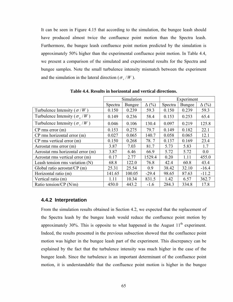
65
It can be seen in Figure 4.15 that according to the simulation, the bungee leash should
have produced almost twice the confluence point motion than the Spectra leash.
Furthermore, the bungee leash confluence point motion predicted by the simulation is
approximately 50% higher than the experimental confluence point motion. In Table 4.4,
we present a comparison of the simulated and experimental results for the Spectra and
bungee samples. Note the small turbulence intensity mismatch between the experiment
and the simulation in the lateral direction ( Wv /σ ).
Table 4.4. Results in horizontal and vertical directions.
Simulation Experiment Spectra Bungee ∆ (%) Spectra Bungee ∆ (%)
Turbulence Intensity ( W/σ ) 0.150 0.239 59.3 0.150 0.239 59.3 Turbulence Intensity ( Wu /σ ) 0.149 0.236 58.4 0.153 0.253 65.4 Turbulence Intensity ( Wv /σ ) 0.046 0.106 130.4 0.097 0.219 125.8 CP rms error (m) 0.153 0.275 79.7 0.149 0.182 22.1 CP rms horizontal error (m) 0.027 0.065 140.7 0.058 0.065 12.1 CP rms vertical error (m) 0.150 0.268 78. 7 0.137 0.169 23.4 Aerostat rms error (m) 3.87 7.03 81.7 5.73 5.83 1.7 Aerostat rms horizontal error (m) 3.87 6.46 66.9 5.72 5.72 0.0 Aerostat rms vertical error (m) 0.17 2.77 1529.4 0.20 1.11 455.0 Leash tension rms variation (N) 68.8 122.0 76.8 42.4 60.8 43.4 Global ratio aerostat/CP (m) 25.31 25.54 0.9 38.42 32.10 -16.4 Horizontal ratio (m) 141.65 100.05 -29.4 98.65 87.63 -11.2 Vertical ratio (m) 1.11 10.34 831.5 1.42 6.57 362.7 Ratio tension/CP (N/m) 450.0 443.2 -1.6 284.3 334.8 17.8
4.4.2 Interpretation
From the simulation results obtained in Section 4.2, we expected that the replacement of
the Spectra leash by the bungee leash would reduce the confluence point motion by
approximately 30%. This is opposite to what happened in the August 11th experiment.
Indeed, the results presented in the previous subsection showed that the confluence point
motion was higher in the bungee leash part of the experiment. This discrepancy can be
explained by the fact that the turbulence intensity was much higher in the case of the
bungee leash. Since the turbulence is an important determinant of the confluence point
motion, it is understandable that the confluence point motion is higher in the bungee

66
sample. Furthermore, this trend is similar for the simulation and experiment and the
bungee actually performed better than what the simulation predicted. This makes us
believe that for comparable turbulence intensities, the bungee leash would have decreased
the confluence point motion.
We are also interested in narrowing down the source of the discrepancy between the
simulation and the experiment performed in the previous subsection. We would like to
ensure that the discrepancy between the bungee experimental and simulated confluence
point motion is not due to the use of an incorrect leash model in the simulation. To do
this, we modify the simulation to remove the aerostat and wind model, and replace them
by applying the measured leash tension (magnitude and direction) at the top of the leash
in the simulation. This is done for Sample #10 (Spectra leash) and Sample #12 (bungee
leash). We then compare the payload error produced by the simulation to the measured
payload error. As we can see in Figures 4.16 and 4.17, the good matches obtained suggest
that the remaining parts of the simulation (all elements other than the wind and aerostat
model) are a good match to reality. This is equally true for the Spectra and bungee
leashes.
We therefore conclude that the discrepancy between the simulation and experiment must
originate either in the wind or the aerostat model. In fact, we have good reasons to believe
that part of the problem lies in the turbulence model. Indeed, we note from Table 4.4 that
the simulation appears to over predict the leash tension rms variation. This is something
that has been seen in previous Penticton experiments and other projects using the LAR
simulation have associated this issue to the turbulence model. It therefore appears that
with an improved turbulence model, we will likely get better match between simulation
and reality.
Because of the difference in the wind conditions of the Spectra and bungee leash flight
parts, it is impossible to use the measurements of August 11th to validate or invalidate the
system improvements that could be expected by the replacement of the Spectra leash by a
bungee leash. However, two reasons lead us to believe that, for comparable aerostat wind
conditions, the bungee leash system would reduce the payload motion: (a) this is
predicted by the simulations done in this chapter and Figures 4.16 and 4.17 demonstrates

67
the validity of the Spectra and bungee models, and (b) the ratio of leash tension rms to
payload rms error is higher for the bungee leash, indicating that the bungee leash
performs better than the Spectra leash in reducing the transmission of perturbations
coming from the aerostat.
Fig. 4.16. Simulation of Spectra Sample #10 with experimental top leash tension.
In order to make a stronger conclusion regarding the performance of the bungee leash, it
would have been best to perform additional bungee experiments until more representative
wind conditions could be obtained. This turned out not to be possible since the retrieval
procedure with the bungee leash was judged to be too hazardous to allow further flights.
Indeed, during the last bungee experiment on October 13th, the aerostat was flown with
the bungee leash for almost six hours waiting for good wind conditions. The aerostat flew
for so long that upon retrieval, the backup and bungee cables were badly twisted together.
In order to untangle them, the backup cable had to be disconnected, leaving the aerostat
secured only with the bungee. This was risky since the factor of safety of the bungee
cable is only 1.5. A photograph taken during August 11th experiment is shown in.
Figure 4.18 and shows what this tangling looks like. Note that in this photograph, the
backup cable is much less twisted than during the October 13th experiment.

68
Fig. 4.17. Simulation of bungee Sample #12 with experimental top leash tension.
Fig. 4.18. Example of backup cable tangling (August 11th).

69
4.5 Conclusion
In this section, we summarize the advantages and the disadvantages of using a bungee
leash in the LAR multi-tethered aerostat system. The advantages of a bungee leash would
be the reduction of the payload motion frequency as well as the reduction of the payload
rms error by approximately 30% in a system with sufficient lift (see Figure 4.8). As was
discussed in Subsection 4.2.3, reducing the payload motion frequency would improve the
effectiveness of other active methods such as the confluence point mechanism or winch
control.
The expected reduction in payload motion of 30% with the bungee leash arrangement
designed in this chapter is far from the 90% reduction presented in Figure 2.5. The reason
for this discrepancy comes from the material limitation. Indeed, there is a practical lower
limit to the bungee cable stiffness, which is approximately 40 N/m in our case, since the
bungee must be strong enough to transmit the lift of the aerostat. To further decrease the
stiffness of the bungee leash, we would have to increase its length and therefore add
substantially more weight to the system. Reducing its diameter would not be an option
since this would decrease the safety factor of the cord.
As we mentioned earlier, the weight added by a bungee leash is a serious disadvantage of
this approach. For the experiment performed in Penticton, the bungee cable added 28 kg
to the system and hence doubled the leash weight. A longer bungee leash would easily
have tripled or quadrupled the leash weight. In principle, we can size the LAR aerostat to
compensate for additional weight, so this is not an unresolvable problem. However, the
cost of an aerostat increases with its size. It would be important to further study the
performance improvement and weight of the different possible techniques and to choose
wisely which ones warrant being implemented in the LAR multi-tethered aerostat system.
The increased complication of the aerostat launching and retrieval procedures is another
big drawback of the bungee leash approach. For reasons of safety and power and data
transmission, we required a second cable parallel to the bungee cable. To cope with
potential conductor breakage, we also had to design a backup power and data collection
system. In at least one instance, the bungee and the safety cable became badly entangled.

70
This tangling made the retrieval procedure so hazardous that we stopped further bungee
experiments. In the cables used for bungee jumping, the safety cable is generally a strap
wrapped around the rubber core. If we could power the ballonet platform through such a
strap and find a way to roll the bungee leash onto a winch, we might have a safer setup
that would enable releasing and retrieving of the bungee leash.
Finally, it should be noted that the use of a bungee leash would significantly increase the
required maintenance of the LAR multi-tethered aerostat system. Indeed, since the rubber
deteriorates with time due to factors such as ambient moisture, sun exposure and mean
elongation, the bungee leash would have to be replaced every one or two years. As
bungee cables are relatively expensive, this would increase the operational cost of the
LAR facility. As an example, BCI provided an estimate of the cost of a bungee cord that
would sustain the LAR full-scale aerostat lift (estimated at 107 kN). Using multiple off-
the-shelf bungee cords attached together with customized attachments, BCI could provide
us with a 24-metre bungee arrangement 30 times stronger than the custom-made bungee
cord used for the Penticton experiments. This full-scale bungee leash would cost
approximately 40,000 USD.
Presently, the bungee leash approach seems heavy, complex and expensive for the
relatively modest improvement in performance in the multi-tethered aerostat system. For
these reasons, we believe that the addition of a bungee leash in the LAR system is of
questionable benefit. Other approaches for improving the system performance may prove
more worthwhile. Perhaps the bungee leash approach could be revisited if those other
approaches turn out to be fruitless.

71
Chapter 5
Design of a Variable Leash Attachment Point Mechanism
5.1 Introduction
In Chapter 3, we evaluated three approaches to actively reduce the confluence point
motion of the multi-tethered aerostat system: leash attachment point pitch control, fin
deflection pitch control and active heave compensation of the leash. In that chapter, we
concluded that only the leash attachment point controller would be further investigated.
This controller displaces the leash attachment point on the lower part of the harness in
order to control the aerostat pitch. To perform that in practice, a variable leash attachment
mechanism must be devised.
In this chapter, we design this mechanism in greater detail. The purpose of this exercise is
not the construction of the mechanism or the implementation of the controller but a more
accurate appraisal of its practicalities and the enhancement of the corresponding
simulation model. We set out to design a mechanism that would control the location of
the leash attachment point in response to errors in the payload altitude, as was done with
controller #2 of Table 3.1 in Section 3.2.
The structure of this chapter is as follows: In Section 5.2, we select the different
components of the variable leash attachment mechanism. The mechanism arrangement is
presented in Section 5.3 and implemented in the simulation in Section 5.4. Finally, some
design issues are discussed in Section 5.5.

72
5.2 Component Selection
The variable leash attachment mechanism is essentially a pulley driven by a motor that
rolls along the aerostat harness (see Figure 5.1). The speed of the motor is controlled by a
servo amplifier located on the aerostat ballonet platform. Power and control signals to the
amplifier are provided from the ground through electrical conductors in the leash and
central tether. In this section, we select the main components of the mechanism, which
include: a pulley, a motor and gear train as well as an amplifier. To implement this
mechanism in the Penticton facility, the aerostat harness would have to be modified. The
lower loop on each side of the harness would have to be merged in a single loop on which
the mechanism could travel.
Fig. 5.1. Location of the leash attachment mechanism.
5.2.1 Pulley
From the simulations performed in Section 3.2, we find that when we use the pitch
controller #2 on the baseline system, the tension difference ∆T in the harness reaches a
maximum value of 2.2 KN. Wrapping the harness on a single pulley would then likely
lead to slippage. To avoid this, we design a double pulley (see Figure 5.2) that reels in the
harness on one side while the other side releases it. It should be noted that due to the

73
lateral offset of the two cable elements, the mechanism would tend to twist so that the two
cables become aligned.
Pulley characteristics Hole diameter 15 mmPulley diameter 68 mmFlange diameter 110 mmSpace between flanges 20.5 mmFlanges width 3 mmTotal pulley width 50 mmWeight estimate 0.75 Kg
Fig. 5.2. Pulley schemas and characteristics.
The outside diameter of the pulley is set at 68 mm. We saw in Section 3.2 that the pitch
controller #2 needs a total displacement of 1.4 metres on the harness. Therefore, the other
dimensions of the pulley are chosen to fit 1.4 metres of 6-mm spectra cable on each side
on two layers. Because of this second layer, we use a value of 80 mm for the outside
diameter when we verify the motor torque requirements in the next subsection.
5.2.2 Servo Motor
Based on the preliminary evaluation of controller #2, the selected motor would have to
hold a maximum tension of 2.2 kN at a maximum speed of 0.68 m/s and therefore
produce a maximum power of 1.5 kW. In order to minimize the size of the motor, we
inspect the harness tension difference and speed curves presented in Figure 5.3 to see if
we could trade off some system performance for significant weight reduction.
Based on Figure 5.3, the size of the motor is minimized by two different ways. The first
way does not trade off performance and consists of selecting a motor that could exert a
continuous tension of 1.75 kN and a peak tension of 2.2 kN. Indeed, we find that the
peaks at 1.75 kN are approximately five seconds long and therefore it is reasonable to use
this value as the requirement for the motor continuous range. The second way to decrease
74
the motor size is to reduce its maximum speed from 0.68 m/s to 0.28 m/s. This speed
reduction reduces the motor weight at very little penalty since the mechanism speed only
exceeds 0.28 m/s two percent of the time. In fact, by implementing a speed limit of
0.28 m/s into controller #2, the simulation shows that we would reduce the payload rms
motion from 19 cm in the baseline system to 8 cm (compared to 7 cm for the controller
without the speed limit).
Fig. 5.3. Harness tension difference and speed for controller #2.
To satisfy these tension and speed requirements, we select the BSM80N-150AA AC
Brushless Servo Motor from Baldor Electric Company [38] as it produces a torque of
1.65 Nm at a rotational speed of 3500 rpm. Since the pulley has two layers, we use its
minimal outside diameter of 68 mm to verify the speed requirement and its maximal
outside diameter of 80 mm to verify the tension requirements. With a gear ratio of 44.4:1
and a pulley diameter of 68 mm, a speed of 0.28 m/s is achieved with this motor. For a
pulley diameter of 80 mm, it produces a maximum continuous tension of 1.83 kN, which
fits our requirement. Finally, the required peak tension of 2.2 kN corresponds to a motor

75
torque of 2 Nm which is also perfectly achievable by the BSM80N-150AA. Figure 5.4
shows some characteristics of this motor:
BSM80N-150AA Servo Motor Characteristics Continuous stall torque 1.65 NmContinuous stall current 3.05 AmpsPeak torque 6.60 NmRotational speed 3500 rpmCurrent for a torque of 2 Nm 3.6 AmpsWeight 3.63 Kg
Fig. 5.4. BSM80N-150 motor and characteristics [38].
5.2.3 Servo Amplifier
In order to control the speed of the motor, we use Baldor’s FlexDriveII FDH2A05TR-
EN23 AC servo amplifier [38]. Figure 5.5 shows some characteristics of this device:
FDH2A05TR-EN23 Characteristics Input Voltage 230 VAC single ΦCommand Signal ±10 VDCMaximum current 5 AmpsDimensions 15.3 x 9.3 x 20.5 cm3
Weight 3 kg
Fig. 5.5. FDH2A05TR-EN23 amplifier and characteristics [38].
This amplifier controls the speed of the motor according to a command signal that would
be generated by the PID controller. Note that the FlexDriveII servo amplifier accepts
either a ±10 VDC command signal or a pulse and direction input. As mentioned
previously, the power and command signal would be provided through the central tether
and the leash (a total length of 370 metres). Therefore, in addition to the component
weight, the variable leash attachment point system also adds weight due to electrical
power wires.

76
In order to estimate this weight, we start with the assumption that three 370-m wires are
required to provide a ground and supply the servo amplifier with 230 VAC single phase
at 3.6 Amps (the maximum motor current). If three AWG 12 copper wires were used,
with properties taken from [39], these conductors would weigh:
3389204
002052.0370332
≈⋅⋅
⋅⋅==πρLAW kg
Since the resistance of the AWG 12 wire is 5.32 ohms per km, the voltage drop at peak
current in the conductors would be:
1.76.337.032.5 ≈⋅⋅==∆ RIV Volts
which corresponds to a drop of 3.1% relative to the 230 VAC supply voltage. For
performance issues, the National Electric Code recommends a maximum voltage drop of
3% [40]. Therefore, the maximum voltage drop obtained with AWG 12 wires is
acceptable.
5.2.4 Gearing
In Subsection 5.2.2, we saw that the gear ratio required to reduce the motor speed is
44.4:1. Since the motor rotational speed of 3500 rpm is relatively high, we first use a 10:1
precision gearhead, the Mijno MRP 090 [41]. To achieve the remaining 4.4:1 gear ratio
and transmit the rotation from the motor axis to the pulley axis, we use one set of bevel
gears followed by one set of spur gears, both supplied by Quality Transmission
Components [42]. Figure 5.6 shows the characteristics of these different gear
components.
Note that the gear efficiencies have not been taken into account when the motor was
selected. The final design of the leash attachment point mechanism should account for
losses in the geartrain. In the next section, we present how the different selected
components are arranged.

77
Mijno MRP 090 Precision Gearhead Characteristics Input Speed 3500 rpm Input Torque 3.5 Nm Gear Ratio 10 :1 Weight 3 kg
QTC MBSG2 Bevel Gears Characteristics Input Torque 24 Nm Gear Ratio 2 :1 Weight 0.72 kg
QTC MSGA1-45 and MSGA1-100 Spur Gears Characteristics Input Torque 44 Nm Gear Ratio 2.22:1 Weight 0.86 kg
Fig. 5.6. Gear components and characteristics. [41][42]
5.3 Mechanism Arrangement
In this section, a preliminary design for the leash attachment point mechanism is
proposed. We first present drawings of the mechanism and then we discuss its main parts.
The proposed mechanism arrangement transmits the rotation of a vertical motor to the
pulley via two sets of gears. Figure 5.7 shows isometric and front views of the
mechanism. Its dimensions are 52x17x10 cm3 and its weight is estimated to be 15 kg (this
excludes the weight of the amplifier and of the conductors). Therefore, the overall system
would add approximately 50 kg to the Penticton multi-tethered aerostat facility.

78
Fig. 5.7. Leash Attachment Point Mechanism.
No stress analysis was performed on the mechanism structure. Therefore, to make sure
that they can support the different forces, the frame and shafts should be more precisely
dimensioned in a future detailed design. Both shafts are fixed: the primary shaft is bolted
while the secondary shaft is embedded. Furthermore, the secondary shaft can be smaller
than the primary shaft since it does not support the aerostat lift. In the present design, the
diameters of the primary and secondary shafts are respectively 15 and 6 millimetres.
The pulley and the large spur gear are machined and bolted together to create the pulley
assembly shown in Figure 5.7. Needle bearings are installed inside the pulley assembly to
permit rotation on the primary shaft. The SKF NA 6902 needle bearing [43], with an
outside diameter of 3 cm, would fit perfectly inside the pulley assembly and support the
79
full lift of the aerostat. In order to centre the pulley on the primary shaft, a SKF 51103
thrust bearing [43] positioned with a collar (not shown in Figure 5.7) would be used on
each side of the pulley assembly.
The large bevel gear and the small spur gear combine to make the bevel gear assembly
(see Figure 5.7). To allow this to spin on the secondary shaft, a SKF NAO 6x17x10 TN
needle bearing [43] would be fit in the assembly. Furthermore, the assembly would be
accurately positioned using a SKF BA 7 thrust bearing [43] on the bevel gear side (not
shown in Figure 5.7).
5.4 Performance
In this section, we evaluate the performance of a variable leash attachment point
controller that uses the mechanism designed in Sections 5.2 and 5.3 and we compare it to
the performance of controller #2 presented in Section 3.2. To accomplish this, we
implement a pitch controller with the variable leash attachment mechanism characteristics
and limitations in the simulation of the baseline system.
The mechanism characteristics and limitations are implemented in the simulation as
follows: (a) the servo amplifier weight of 3 kg is added at the ballonet platform, (b) the
mechanism weight of 15 kg is added at the leash top node, (c) the leash density as well as
the payload weight are increased to account for the added conductor weight of 33 kg, and
finally (d) position and speed limits of respectively ±0.7 m and ±0.28 m/s are
implemented in the controller to limit the motion of the leash attachment point on the
aerostat harness.
We implement a PID controller very similar to controller #2 of Section 3.2 in the baseline
system. This controller stabilizes the payload altitude by varying the leash attachment
point position on the aerostat harness. The only differences between this controller and
controller #2 are the gains of the PID. Indeed, the speed limit imposed here forces us to
reduce the PID gains for the system to remain stable. By optimizing these gains by trial
and error we obtain: kp = 2, ki = 0.8 s-1 and kd = 0.01 second. Figure 5.8 shows the system
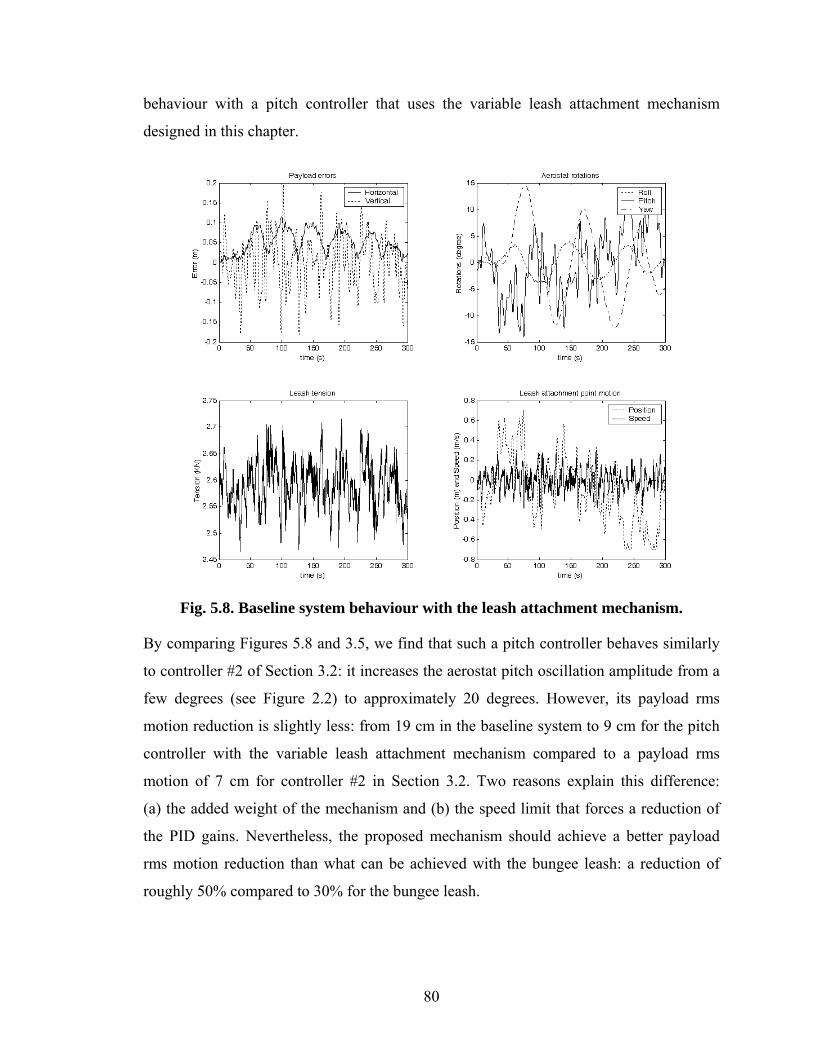
80
behaviour with a pitch controller that uses the variable leash attachment mechanism
designed in this chapter.
Fig. 5.8. Baseline system behaviour with the leash attachment mechanism.
By comparing Figures 5.8 and 3.5, we find that such a pitch controller behaves similarly
to controller #2 of Section 3.2: it increases the aerostat pitch oscillation amplitude from a
few degrees (see Figure 2.2) to approximately 20 degrees. However, its payload rms
motion reduction is slightly less: from 19 cm in the baseline system to 9 cm for the pitch
controller with the variable leash attachment mechanism compared to a payload rms
motion of 7 cm for controller #2 in Section 3.2. Two reasons explain this difference:
(a) the added weight of the mechanism and (b) the speed limit that forces a reduction of
the PID gains. Nevertheless, the proposed mechanism should achieve a better payload
rms motion reduction than what can be achieved with the bungee leash: a reduction of
roughly 50% compared to 30% for the bungee leash.

81
5.5 Design Issues
During this first design iteration of the leash attachment mechanism, two issues were
noted that would have to be addressed in future designs. The first considers the possibility
for unwanted oscillations of the mechanism. The second considers the option of using
batteries to power the mechanism.
5.5.1 Mechanism Oscillation
As can be seen in Figure 5.9, the tension difference in the harness and thus the motor
torque is only counterbalanced by the leash tension acting at an angle θ to the mechanism.
If we neglect the dynamics of the mechanism and take moments about its mass centre, we
find:
θsin)( 12 TLTTrM =−= (5.1)
⎥⎦⎤
⎢⎣⎡ −
= −
TLTTr )(sin 121θ (5.2)
Fig. 5.9. Static equilibrium of the leash attachment mechanism.
As the tension difference in the harness varies from one extreme to another, the
mechanism oscillates to counterbalance it. This oscillation was not modeled in the

82
simulation performed in the previous section and therefore its effect on the controller
performance should be further evaluated in the future. Using Equation 5.2, the
mechanism angle θ was computed for the manoeuvre of Figure 5.8. The mechanism
oscillation is presented in Figure 5.10. From this figure, we note that the amplitude of
oscillation would be approximately ±8o. If it proves to be problematic, there are two ways
to reduce the mechanism oscillation: (a) reducing the pulley diameter and (b) increasing
the moment arm L of the leash tension. The values of r and L used in this exercise were
8 cm and 52 cm, respectively.
Fig. 5.10. Mechanism oscillation for the simulation of Section 5.4.
5.5.2 Battery Power
In Subsection 5.2.3, we estimated the weight of the electrical conductors required to
supply the leash mechanism motor to be approximately 33 kg. Here we investigate the
possibility of instead using batteries to supply power to the motor. In order to estimate the
weight of the batteries required, we assume that Sanyo Twicell HR-DU [44] nickel-metal
hydride batteries would be used. Each of these batteries weighs 178 grams, has a nominal

83
voltage of 1.2 volts and a capacity of 9 amps-hour. Consequently, the energy provided by
a HR-DU cell is 10.8 watts-hour.
For the five-minute manoeuvre of Figure 5.8, the mechanism requires approximately
6 watts-hour. We obtained this energy value by integrating the absolute value of the
instantaneous power, obtained by multiplying the mechanism speed by the tension
difference in the harness. The absolute value of the power is used since it is
conservatively assumed that there is no energy recovery in the system and that generating
negative power consumes as much energy as generating positive power. Therefore, we
estimate that seven HR-DU cells would be needed to power the leash attachment point
mechanism for an hour. Since these cells would only add 1.3 kg to the system, which is
25 times less than added by electrical conductors, and because the experimental flights
are usually no longer than one hour, powering the mechanism with batteries seems to be
an attractive option for testing. The motor and amplifier selected in Section 5.2 would
have to be changed if we chose this option, as they work on AC power.
In the case of the full scale LAR system, we would have to power the mechanism from
the ground through the central tether and the leash. Indeed, since the LAR aerostat system
will be flying for much longer (and indefinite) periods of time, the battery approach
would be infeasible.
5.6 Conclusion
In this chapter, we designed a mechanism that displaces the leash attachment point on the
harness in order to control the pitch of the aerostat. This design was preliminary in nature.
After the implementation of the proposed mechanism into the simulation, we found that
the use of leash attachment pitch control could reduce the payload rms motion by 50%.
This active method looks therefore more promising than the bungee leash approach, for
which we found a payload rms motion reduction of 30% in Chapter 4. However, as we
learned from the bungee leash experiment, pitch control may prove to perform less well
when implemented in practice. It is thus important to further develop leash attachment
pitch control in order to test it on a tethered aerostat system.

84
Chapter 6
Conclusion
In this thesis, we considered different ways of reducing the payload motion of the LAR
multi-tethered aerostat system. By simulating this system, it was first discovered that
most of the payload perturbations were produced by the aerostat and transmitted to the
payload through the leash. Indeed, by replacing the simulated aerostat of the baseline case
by a constant force equal in magnitude and direction to the mean top leash tension of this
same case, we found that the payload rms motion was reduced by nearly 95 percent. A
similar test in which the aerostat was replaced by a constant leash tension magnitude
while allowing its direction to vary as in the baseline case showed that the variations in
the leash tension magnitude were responsible for approximately 75 percent of the payload
rms motion. For this reason, this thesis focused on reducing variations in the leash tension
magnitude as a way of reducing the payload motion.
By varying the leash properties of the baseline system in the simulation, it was discovered
that among its length, its stiffness and its damping, the leash property that has the largest
effect on the payload motion is its stiffness. Indeed, by sufficiently reducing the leash
stiffness in the simulation, the magnitude of the leash tension as seen by the payload
became nearly constant and the payload rms motion was reduced by 75 percent. In order
to reduce the leash stiffness in the physical system, three passive methods were
considered: (a) a constant force spring, (b) a passive heave compensator and (c), a bungee
leash.
A constant force spring is a roll of prestressed strip that exerts a nearly constant
restraining force to resist uncoiling. As expected, it was found by simulating the system

85
that the payload motion could be reduced by 75 percent if we placed such a spring at the
base of the leash. However, it was also noted that a constant force spring would require a
travel length of approximately 60 metres and be able to oppose a force of 2.6 kN. Since
such large constant force springs are unavailable, the constant force spring was rejected as
a solution for the LAR multi-tethered system.
A passive heave compensator at the base of the leash would include a pneumatic spring,
an accumulator and a pulley system to increase the mechanism travel length. By
simulating the baseline system with a passive heave compensator with a stiffness of
1 N/m, it was found that the required pretension and travel length would be respectively
2.6 kN and 64 metres, and the rms motion of the payload would be reduced by 78 percent.
To avoid hitting its stops, the passive heave compensator would have to be used jointly
with a system that would actively control either its pretension or the mean leash tension
with changes in wind speed. The added weight and complexity of the passive heave
compensator were seen as excessive, and this solution was not pursued further.
The last passive method considered to reduce the leash stiffness was the replacement of
the present Spectra leash whose stiffness is 5300 N/m by a bungee leash with a stiffness
of 5 N/m. With the bungee leash, simulations showed that the payload rms motion would
be reduced by 63 percent. Since this method seemed very promising and simple, we chose
to implement it on the one-third-scale test platform in Penticton, British Columbia. Due to
the limited lift of the Penticton system, we were forced to use a half Spectra – haft bungee
leash with a stiffness of 40 N/m. An additional safety cable was used in parallel with the
bungee part to (a) back the bungee part in case of failure, (b) power the ballonet platform,
and (c) ease the launching and retrieval procedures. By simulating this arrangement, we
expected to observe two things in the experiment: a reduction of the payload rms motion
of 30 percent and a significant reduction of the payload oscillation frequency. The
reduction in payload frequency would greatly simplify its stabilisation by other active
methods.
The experimental results obtained did not demonstrate any reduction in payload rms
motion or frequency with the bungee leash. This was attributed to much higher turbulence
conditions existing during the part of the flight with the bungee leash. However, the

86
bungee leash performed better than what was predicted by the simulation. We concluded
that the available data was not sufficient to validate or invalidate the system
improvements expected with the bungee leash. Nevertheless, the data collected allowed
us to validate the bungee and Spectra leash models, which increased our confidence in the
simulation results. The implementation of a bungee leash on the test platform in Penticton
highlighted some drawbacks of the bungee approach, including its weight and operational
complexity. We concluded that the addition of a bungee leash in the LAR system was of
questionable benefit since it seemed heavy and expensive for a relatively small
improvement in performance.
Two active methods were considered in order to improve the payload stability of the LAR
multi-tethered aerostat system: (a) active constant force spring and (b) aerostat pitch
control.
The active constant force spring approach was derived from an evaluation of an active
heave compensator controlling the leash speed. This consisted of a motor mounted on the
payload used to control the leash speed in order to stabilize the leash tension. Since it is
possible to produce a constant torque by supplying a DC servo motor with a constant
current, we proposed simply using a servo amplifier to ensure that a constant current was
supplied to the motor. With this approach, the performance obtained with a constant force
spring, a reduction of 75 percent of the payload RMS motion (note that this performance
does not take into account the weight of the device), could be achieved with the added
advantage that changes in wind conditions could be compensated for by simply changing
the value of the current set point. However, such a device would add complexity and
weight to the LAR aerostat system, and would require substantial power at the confluence
point, thus leading us to reject this approach.
We investigated two ways of controlling the pitch of a streamlined aerostat: aerostat
tailfin deflection control and leash attachment point control. We found that a tailfin-based
pitch controller might reduce the payload RMS motion by as much as 63 percent.
However, we did not further investigate this approach since it was impossible to test it in
Penticton, as the streamlined aerostat used has fixed inflatable fins.

87
A leash attachment point pitch controller would displace the leash attachment point on the
lower loop of the harness in order to control the aerostat pitch. This mechanism, which
comprises a pulley, a servo motor, a servo amplifier and a geartrain, would be powered
from the ground through the central tether and the leash. We estimated that the overall
weight added by a leash attachment mechanism would be 50 kg, and would lead to a
reduction of 50 percent in the payload rms motion. Finally, we also found that this device
would require substantially less power at the confluence point than the active constant
force spring. The relative simplicity of this active system led us to recommend it for
future detailed investigation.
6.1 Recommendations for Future Work
A number of recommendations for future work are now suggested as worthwhile
continuations of the research performed here.
1. Develop a systematic technique to determine if two data samples provided by the
Penticton facility have comparable aerostat wind conditions.
2. Improve the launching and landing procedures of the bungee experiment. Safety
should be the main concern.
3. Perform additional bungee leash experiments jointly with Spectra leash
experiments at the Penticton facility in order to get two samples with comparable
aerostat lift and wind conditions. Confirm or disprove the simulation results,
which predict a 30% reduction in payload motion with the bungee leash.
4. Use the McGill small-scale facility to obtain reliable and quantitative data on the
effect of the leash length on tether tension and angle variations. These could then
be used in the LAR simulation to predict the resulting payload motion (the McGill
facility is single-tethered; has no payload).

88
5. Perform a detailed design of a passive heave compensator in order to get a better
idea of its weight and complexity.
6. Refine the design of a leash attachment point mechanism. Implement it at the
Penticton facility or at the McGill small-scale facility and test the leash attachment
point pitch controllers.

89
References
[1] R. van de Weygaert, T.S. van Albada., “New Challenges for Cosmology,” The
Westerbork Observatory, Continuing Adventure in Radio Astronomy, Astrophysics
and Space Science Library, Vol. 207, pp. 225-259, 1996.
[2] Legg T.H., “A Proposed New Design for a Large Radio Telescope,” Astronomy
and Astrophysics Supplement Series, Vol. 130, pp. 369-379, 1998.
[3] Schilizzi R.T., “The Square Kilometre Array,” International SKA Project Office,
(http://www.skatelescope.org/).
[4] Hall P.J., “The Square Kilometre Array: An International Engineering
Perspective,” International SKA Project Office, (http://www.skatelescope.org/).
[5] Carlson B. et al., “The Large Adaptive Reflector: a 200-m Diameter, Wideband,
cm-m Wave Radio Telescope,” Proceedings of the SPIE International Symposium
on Astronomical Telescopes and Instrumentation, pp. 33-44, 2000.
[6] Dewdney P.E., Nahon M., and Veidt B., “The Large Adaptive Reflector: A Giant
Radio Telescope with an Aero Twist”, Canadian Aeronautics and Space Journal,
Vol. 48, No. 4, pp. 239-250, 2002.
[7] DeLaurier J.D., “A Stability Analysis for Tethered Aerodynamically Shaped
Balloons,” AIAA Journal of Aircraft, Vol. 9, No. 9, pp. 646-651, 1972.
[8] DeLaurier J.D., “Prediction of Tethered-Aerostat Response to Atmospheric
Turbulence,” AIAA Journal of Aircraft, Vol. 14, No. 4, pp. 407-409, 1977.
[9] Jones S.P., and Krausman J.A., “Nonlinear Dynamic Simulation of a Tethered
Aerostat,” AIAA Journal of Aircraft, Vol. 19, No. 8, pp. 679-686, 1982.

90
[10] Jones S.P., and DeLaurier J.D., “Aerodynamic Estimation Techniques for
Aerostat and Airships,” AIAA Journal of Aircraft, Vol. 20, No. 2, pp. 120-126,
1983.
[11] Badesha S., and Jones S.P., “Aerodynamics of the TCOM 71M Aerostat,” AIAA
Paper 93-4036, pp. 36-42, 1993.
[12] Lambert C., and Nahon M., “Stability Analysis of a Tethered Aerostat,” Journal
of Aircraft, Vol. 40, No. 4, pp. 705-715, 2003.
[13] Redd T., Bland R., and Bennet R.M., “Stability Analysis and Trend Study of a
Balloon Tethered in a Wind, With Experimental Comparisons,” NASA TN D-
7272, Langley Research Center, 1973.
[14] Humphreys D.E., “Validation of the Dynamic Characteristics of a Towed, Scaled
Aerostat,” Proceedings from the 12th AIAA Lighter-Than-Air Systems Technology
Conference, pp. 227-236, 1997.
[15] Jones S.P., and Shroeder L.D., “Nonlinear Dynamics Simulation of a Tethered
Aerostat: A Fidelity Study,” Journal of Aircraft, Vol. 38, No. 1, pp. 64-68, 2001.
[16] Leclaire R.C., and Rice C.B., “The Local Motions of a Payload Supported by a
Tri-Tethered Natural Shape Balloon,” US Air Force Report AFCRL-TR-73-0748,
1973.
[17] Leclaire R.C., and Schumacher H.L., “Local Motions of a Payload Supported by a
Nolaro Tri-Tethered Balloon,” Proceedings of the 8th AFCRL Scientific Balloon
Symposium, Air Force Cambridge Research Lab., Bedford, MA, pp. 233-255,
1974.
[18] Le Coroller H., Dejonghe J., Arpesella C., Vernet D., and Labeyrie A., “Tests
with a Carlina-Type Hypertelescope Protototype,” Astronomy and Astrophysics,
Vol. 426, pp. 721-728, 2004.
[19] Fitzsimmons J.T., Veidt B., and Dewdney P.E., “Steady-State Analysis of the
Multi-Tethered Aerostat Platform of the Large Adaptive Reflector Telescope,”
Proceedings of the SPIE International Symposium on Astronomical Telescopes
and Instrumentation, 2000.

91
[20] Nahon M., “Dynamics and Control of a Novel Radio Telescope Antenna,” A
Collection of the AIAA Modeling and Simulation Technologies Conference
Technical Papers, pp. 214-222, 1999.
[21] Nahon M., Gilardi G., and Lambert C., “Dynamics and Control of a Radio
Telescope Receiver Supported by a Tethered Aerostat,” AIAA Journal of
Guidance, Dynamics and Control, Vol. 25, No. 6, pp. 1107-1115, 2002.
[22] Lambert C., “Dynamics Modeling and Conceptual Design of a Multi-Tethered
Aerostat System,” M.Sc. Thesis, Dept. of Mechanical Engineering, University of
Victoria, Victoria, BC, Canada, Jan. 2002.
[23] Lambert C., Saunders A., Crawford C. and Nahon M., “Design of a One-Third
Scale Multi-Tethered Aerostat System for Precise Positioning of a Radio
Telescope Receiver,” CASI Flight Mechanics and Operations Symposium,
Montreal, Canada, 2003.
[24] Nahon M., Lambert C., Chalmers D., and Bo W., “Model Validation and
Performance Evaluation for the Multi-Tethered Aerostat Subsystem of the Large
Adaptive Reflector,” Experimental Astronomy, 2005.
[25] Niedzwecki J.M., and Thampi S.K., “Heave Compensated Response of Long
Multi-Segment Drill Strings,” Appl. Ocean Res., Vol. 10, pp. 181-190, 1988.
[26] Hover F.S., Grosenbaugh M.A., and Triantafyllou M.S., “Calculation of Dynamic
Motions and Tension in Towed Underwater Cables,” IEEE Journal of Oceanic
Engineering, Vol. 19, pp. 449-457, 1994.
[27] Driscoll F.R., Nahon M., and Lueck R.G., “A comparison of Ship-Mounted and
Cage-Mounted Passive Heave Compensation System,” Journal of Offshore
Mechanics and Artic Engineering, Vol.122, pp. 214-221, 2000.
[28] Driscoll F.R., Buckham B., and Nahon M., “Numerical Optimization of a Cage-
Mounted Passive Heave Compensation System,” Proceedings of Oceans’2000,
2000.
[29] Eide L., “Modeling and Control of a Vertically Tethered Marine Platform Using
an Active Heave Compensation System,” M.Sc. Thesis, Dept. of Ocean
Engineering, Florida Atlantic University, Boca Raton, Florida, USA, Dec. 2003.
[30] The Cortland Companies, http://www.thecortlandcompanies.com.

92
[31] Press W.H., Teukolsky S.A., Vetterling W.T., and Flannery B.P., Numerical
Recipes in C, Cambridge University Press, Cambridge, England, U.K., pp. 710-
714, 1992
[32] Stock Drive Products – Sterling Instruments, http://www.sdp-si.com.
[33] Materials group, Department of Engineering, University of Cambridge,
http://www-materials.eng.cam.ac.uk/mpsite/short/OCR/ropes/default.html
[34] Teorodescu A., “Analysis of an Aerostat Harness,” B.Eng. Thesis, Department of
Mechanical Engineering, McGill University, 2005.
[35] Nasar S. A., Electric Machines and Power Systems - Volume 1, McGraw-Hill,
New-York NY, 1995.
[36] Aerostar International Inc., http://www.aerostar.com/.
[37] Bungee Consultants International, http://www.bungeeconsultants.com/.
[38] Baldor Electric Company, http://www.baldor.com.
[39] Floyd T. L., Electric Circuit Fundamentals, Sixth Edition, Prentice Hall, 2003.
[40] National Fire Protection Association, National Electric Code 2002, Thomson
Delmar Learning, 2001.
[41] Mijno Precision Gearing, http://www.mijno.com.
[42] Quality Transmission Components, http://www.qtcgears.com.
[43] SKF Group, http://www.skf.com.
[44] Sanyo, http://sanyo.com.