a study of lateral vehicle motion - · pdf file1 a study of lateral vehicle motion presented...
TRANSCRIPT
1
A Study of Lateral Vehicle Motion
Presented by:John & Jeremy DailyJackson Hole Scientific Investigations, Inc
Nate ShigemuraTraffic Safety Group
9/26/2004©John Daily, Nathan Shigemura, Jeremy DailyPage 2
Overview
1. Road Evidence– Spin examples– Critical Speed Yaws– Turning and Braking
2. Definitions3. Critical Speed Formula4. Drag Factors and Skid Testing5. Lane Changes
2
9/26/2004©John Daily, Nathan Shigemura, Jeremy DailyPage 3
Overview
6. Testing and Instrumentation7. Dynamic Roadway Marking System8. Data Analysis and Reduction9. Validation of Lane Change Equation10. Derivation of Critical Speed Yaw
Formulation11. Summary and Questions
9/26/2004©John Daily, Nathan Shigemura, Jeremy DailyPage 4
Road Evidence
• Maximum performance lateral maneuvers will saturate one or more of the tires of the vehicle.
• Because lateral motion happens concurrently with forward motion, any saturated tires will leave curving marks on the road.

3
9/26/2004©John Daily, Nathan Shigemura, Jeremy DailyPage 5
Road Evidence
• Our ability to interpret these curving tire marks will allow us to chose a proper method for speed analysis.
• We will examine several different types of curving tire mark evidence in the following slides.
9/26/2004©John Daily, Nathan Shigemura, Jeremy DailyPage 6
Road Evidence - Spins
• A spin is a vehicle motion characterized by relatively high angular velocities.
• A vehicle may spin as a result of inappropriate steering, especially on low coefficient surfaces.
• A vehicle may also enter a spin as the consequence of a collision.
• Uneven braking may also result in a spin.

4
9/26/2004©John Daily, Nathan Shigemura, Jeremy DailyPage 7
Emergency Brake Spin• If the emergency brake only
is used, the vehicle will tend to spin around.
• A combined speed technique may be used to analyze speed.
• The vehicle will track straight for a distance and will then rotate.
• The straight portion may be calculated with a straightforward speed equation, while the spin portion may be calculated with the spin analysis.
9/26/2004©John Daily, Nathan Shigemura, Jeremy DailyPage 8
Road Evidence - Spins
• This is a steering induced spin.
• A spin analysis, such as was presented in Special Problems 2003, would be appropriate for speed analysis.
5
9/26/2004©John Daily, Nathan Shigemura, Jeremy DailyPage 9
Road Evidence - Spins
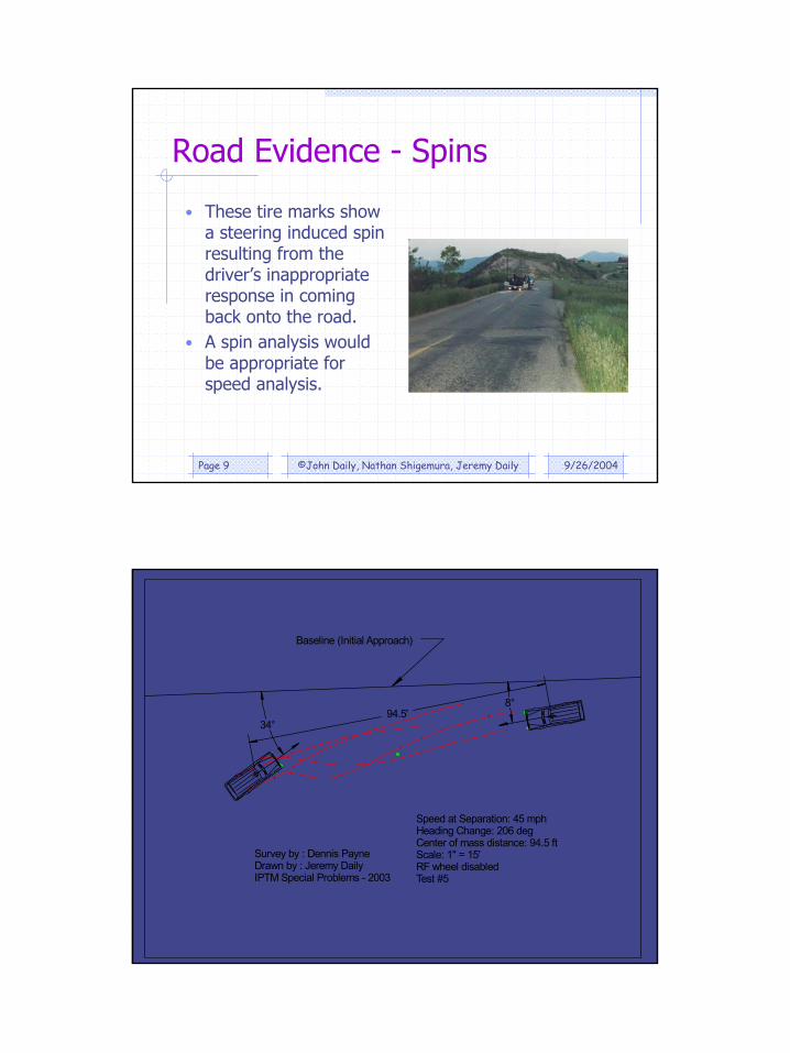
• These tire marks show a steering induced spin resulting from the driver’s inappropriate response in coming back onto the road.
• A spin analysis would be appropriate for speed analysis.
9/26/2004©John Daily, Nathan Shigemura, Jeremy DailyPage 10
94.5'34°
8°
Speed at Separation: 45 mphHeading Change: 206 degCenter of mass distance: 94.5 ftScale: 1" = 15'RF wheel disabledTest #5
Survey by : Dennis PayneDrawn by : Jeremy DailyIPTM Special Problems - 2003
Baseline (Initial Approach)

6
9/26/2004©John Daily, Nathan Shigemura, Jeremy DailyPage 11
Pit-5, No RF brake
-280-240-200-160-120-80-40
04080
120160200240280320
12 13 14 15 16 17 18 19 20
Time, Seconds
Hea
ding
ang
le, d
egre
es
-20020406080100120140160180200220240260280
Yaw
ang
le R
ate,
deg
/sec
Heading Change 216 degrees
VC3000 Data aquired and reduced by Wade Bartlett
9/26/2004©John Daily, Nathan Shigemura, Jeremy DailyPage 12
Road Evidence - Spins
• Angular velocity for spins are typically on the order of 100 degrees per second or higher.
7
9/26/2004©John Daily, Nathan Shigemura, Jeremy DailyPage 13
Road Evidence – Critical Speed Yaw - Definitions
• Yaw refers to the orientation of the vehicle.• Specifically, the heading of the vehicle is not
co-linear with the velocity vector of the vehicle.
• The evidence showing this are the tire scuffs on the road.
• The rear tires track outside the corresponding front tires.
9/26/2004©John Daily, Nathan Shigemura, Jeremy DailyPage 14
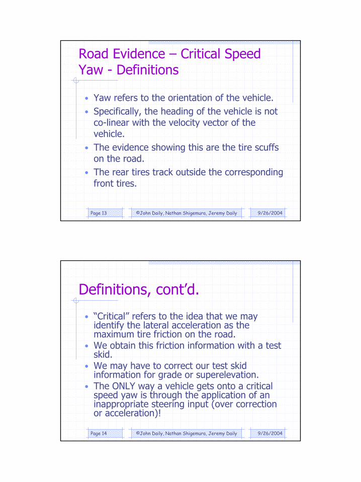
Definitions, cont’d.
• “Critical” refers to the idea that we may identify the lateral acceleration as the maximum tire friction on the road.
• We obtain this friction information with a test skid.
• We may have to correct our test skid information for grade or superelevation.
• The ONLY way a vehicle gets onto a critical speed yaw is through the application of an inappropriate steering input (over correction or acceleration)!
8
9/26/2004©John Daily, Nathan Shigemura, Jeremy DailyPage 15
Road Evidence – Critical Speed Yaw
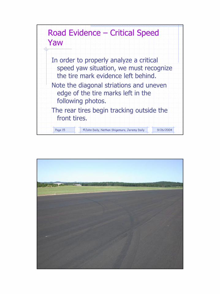
In order to properly analyze a critical speed yaw situation, we must recognize the tire mark evidence left behind.
Note the diagonal striations and uneven edge of the tire marks left in the following photos.
The rear tires begin tracking outside the front tires.
9/26/2004©John Daily, Nathan Shigemura, Jeremy DailyPage 16
9
9/26/2004©John Daily, Nathan Shigemura, Jeremy DailyPage 17
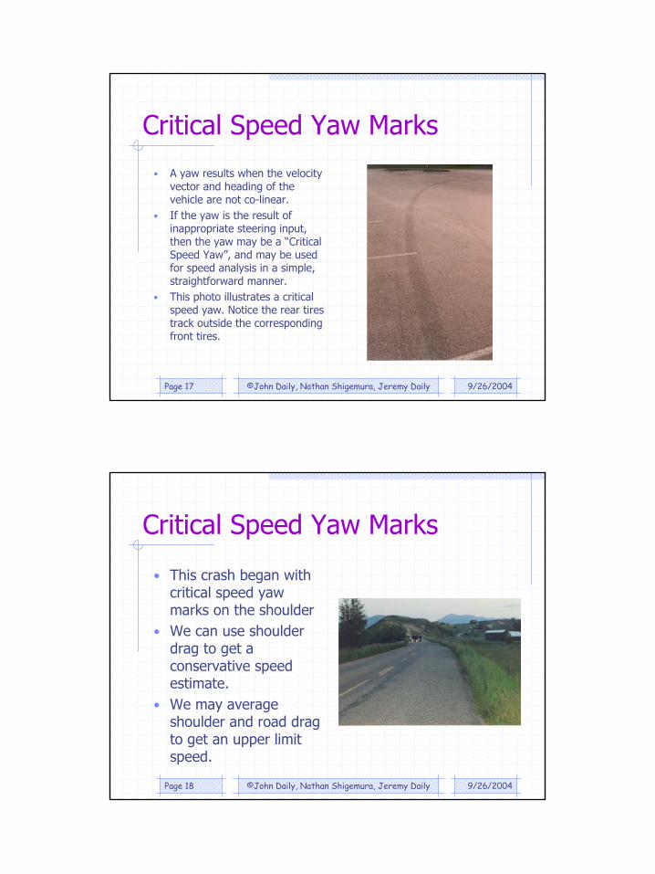
Critical Speed Yaw Marks
• A yaw results when the velocity vector and heading of the vehicle are not co-linear.
• If the yaw is the result of inappropriate steering input, then the yaw may be a “Critical Speed Yaw”, and may be used for speed analysis in a simple, straightforward manner.
• This photo illustrates a critical speed yaw. Notice the rear tires track outside the corresponding front tires.
9/26/2004©John Daily, Nathan Shigemura, Jeremy DailyPage 18
Critical Speed Yaw Marks
• This crash began with critical speed yaw marks on the shoulder
• We can use shoulder drag to get a conservative speed estimate.
• We may average shoulder and road drag to get an upper limit speed.
10
9/26/2004©John Daily, Nathan Shigemura, Jeremy DailyPage 19
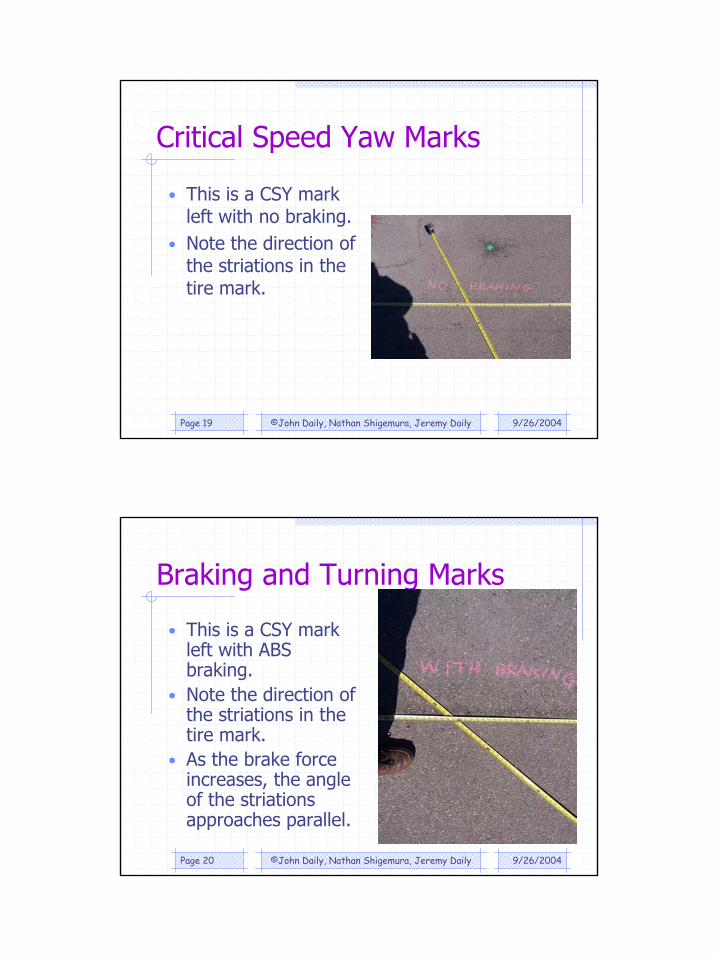
Critical Speed Yaw Marks
• This is a CSY mark left with no braking.
• Note the direction of the striations in the tire mark.
9/26/2004©John Daily, Nathan Shigemura, Jeremy DailyPage 20
Braking and Turning Marks
• This is a CSY mark left with ABS braking.
• Note the direction of the striations in the tire mark.
• As the brake force increases, the angle of the striations approaches parallel.
11
9/26/2004©John Daily, Nathan Shigemura, Jeremy DailyPage 21
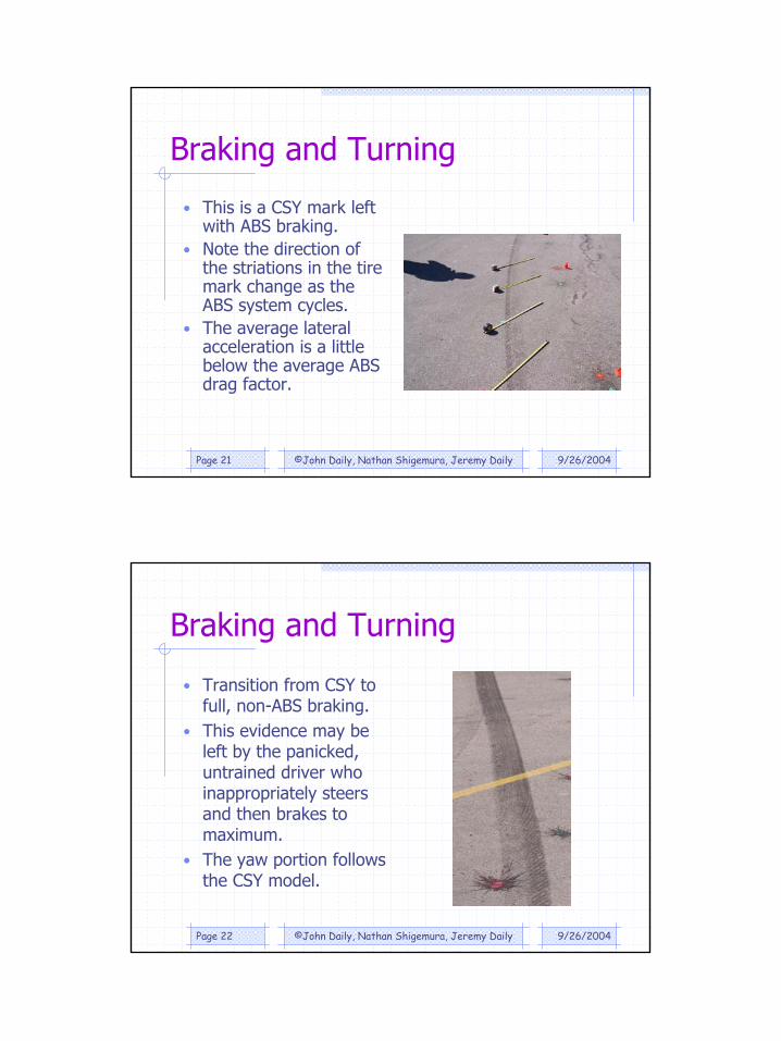
Braking and Turning
• This is a CSY mark left with ABS braking.
• Note the direction of the striations in the tire mark change as the ABS system cycles.
• The average lateral acceleration is a little below the average ABS drag factor.
9/26/2004©John Daily, Nathan Shigemura, Jeremy DailyPage 22
Braking and Turning
• Transition from CSY to full, non-ABS braking.
• This evidence may be left by the panicked, untrained driver who inappropriately steers and then brakes to maximum.
• The yaw portion follows the CSY model.

12
9/26/2004©John Daily, Nathan Shigemura, Jeremy DailyPage 23
Braking and Turning
9/26/2004©John Daily, Nathan Shigemura, Jeremy DailyPage 24
Braking and Turning• Controlled braking and turning
by a trained driver. Rear ABS only.
• The inside mark is a skid, with longitudinal striations.
• The rear tires track outside the corresponding front tires.
• The outside tire marks show diagonal striations.
• May NOT use the CSY analysis with a full drag factor.
• Lateral acceleration is significantly lower than the full drag factor.
• Evidence does NOT support the CSY analysis. A skid analysis would be more appropriate.
13
9/26/2004©John Daily, Nathan Shigemura, Jeremy DailyPage 25
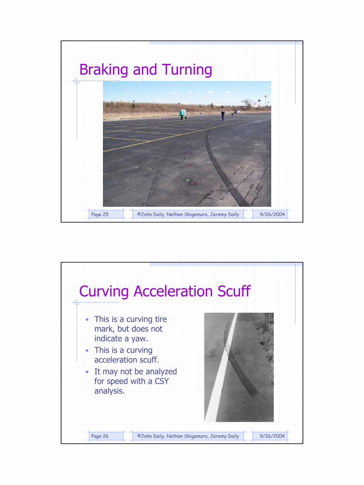
Braking and Turning
9/26/2004©John Daily, Nathan Shigemura, Jeremy DailyPage 26
Curving Acceleration Scuff
• This is a curving tire mark, but does not indicate a yaw.
• This is a curving acceleration scuff.
• It may not be analyzed for speed with a CSY analysis.

14
9/26/2004©John Daily, Nathan Shigemura, Jeremy DailyPage 27
Speed Determination with CSY
• The equation for determining speed from CSY is based upon the concepts of Uniform Circular Motion.
• We make the assumption the vehicle will actually move in a decreasing spiral, because the vehicle is slowing as it progresses through the yaw.
• We may further assume the vehicle trajectory may be approximated as a series of circular arcs.
• These arcs will progressively decrease in radius.
9/26/2004©John Daily, Nathan Shigemura, Jeremy DailyPage 28
Critical Speed Yaw of 2003 Chevy Malibu(VC3000 Computer)
-0.2
0
0.2
0.4
0.6
0.8
1
1.2
13 14 15 16 17 18 19
Time
G's Longitudinal
Lateral
Post Yaw Braking
Initial value as calculated: 0.26
15
9/26/2004©John Daily, Nathan Shigemura, Jeremy DailyPage 29
Speed Determination with CSY
• We may also assume the lateral acceleration factor may be determined through skid testing.
• Finally, we must show the vehicle is in equilibrium. In other words, the vehicle is in a steady state cornering condition.
• If this steady state condition is met, then the lateral acceleration stays at a constant level for some time.
• All of these concepts will be more fully explored by the presentation tomorrow…
9/26/2004©John Daily, Nathan Shigemura, Jeremy DailyPage 30
Speed Determination with CSY
• The same concepts we use to analyze speed from a CSY analysis have been historically used by Highway Engineers to design roads.
• In the 1965 “Blue Book” (AASHO), pg 152, we may find the following equation:

16
9/26/2004©John Daily, Nathan Shigemura, Jeremy DailyPage 31
RV
RVfe
15
067.0
2
2
=
=+
This Reduces to: RfS 86.3=
Copyright © 2004 by John & Jeremy Daily & Nathan ShigemuraCopyright © 2004 by John & Jeremy Daily & Nathan Shigemura 3232
Critical Speed Yaw DerivationCritical Speed Yaw Derivation
Recall the definition of Vectors:Recall the definition of Vectors:Quantity that possesses both MAGNITUDE and Quantity that possesses both MAGNITUDE and DIRECTIONDIRECTION..
Recall the definition of Velocity:Recall the definition of Velocity:A change in DISPLACEMENT with respect to a A change in DISPLACEMENT with respect to a change in TIMEchange in TIME..
Recall the definition of Acceleration:Recall the definition of Acceleration:A change in VELOCITY with respect to a change in A change in VELOCITY with respect to a change in TIMETIME..

17
Copyright © 2004 by John & Jeremy Daily & Nathan ShigemuraCopyright © 2004 by John & Jeremy Daily & Nathan Shigemura 3333
Critical Speed Yaw Derivation Critical Speed Yaw Derivation (cont.)(cont.)
Velocity and Acceleration are vector Velocity and Acceleration are vector quantities.quantities.Thus, if the MAGNITUDE of a moving Thus, if the MAGNITUDE of a moving vehicle’s velocity changes, there is an vehicle’s velocity changes, there is an Acceleration.Acceleration.And if the DIRECTION of a moving And if the DIRECTION of a moving vehicle changes, there is an vehicle changes, there is an Acceleration (because the velocity is Acceleration (because the velocity is changed).changed).
Copyright © 2004 by John & Jeremy Daily & Nathan ShigemuraCopyright © 2004 by John & Jeremy Daily & Nathan Shigemura 3434
Critical Speed Yaw Derivation Critical Speed Yaw Derivation (cont.)(cont.)
Therefore a vehicle traveling at constant Therefore a vehicle traveling at constant velocity (magnitude) in a curve is velocity (magnitude) in a curve is undergoing an Acceleration (since it’s undergoing an Acceleration (since it’s continually changing directions).continually changing directions).More specifically, it is experiencing a More specifically, it is experiencing a Lateral Acceleration.Lateral Acceleration.

18
Copyright © 2004 by John & Jeremy Daily & Nathan ShigemuraCopyright © 2004 by John & Jeremy Daily & Nathan Shigemura 3535
Critical Speed Yaw Derivation Critical Speed Yaw Derivation (cont.)(cont.)
For a vehicle to move laterally left or right, it requires For a vehicle to move laterally left or right, it requires surface friction.surface friction.More specifically, it requires a force which the surface More specifically, it requires a force which the surface friction will produce in the lateral direction (i.e. friction will produce in the lateral direction (i.e. perpendicular to the longitudinal velocity vector).perpendicular to the longitudinal velocity vector).If the surface friction is greater than the lateral friction If the surface friction is greater than the lateral friction the vehicle is needing to travel in a curving path, the the vehicle is needing to travel in a curving path, the vehicle will be able to successfully negotiate the vehicle will be able to successfully negotiate the curving path.curving path.If the vehicle requires more lateral friction than the If the vehicle requires more lateral friction than the surface can provide, then the vehicle will begin to lose surface can provide, then the vehicle will begin to lose control.control.
Copyright © 2004 by John & Jeremy Daily & Nathan ShigemuraCopyright © 2004 by John & Jeremy Daily & Nathan Shigemura 3636
Critical Speed Yaw Derivation Critical Speed Yaw Derivation (cont.)(cont.)
A vehicle traveling in a curving path is A vehicle traveling in a curving path is experiencing both lateral and experiencing both lateral and longitudinal forces.longitudinal forces.Let’s look at the lateral forces the Let’s look at the lateral forces the vehicle is experiencing.vehicle is experiencing.
19
Copyright © 2004 by John & Jeremy Daily & Nathan ShigemuraCopyright © 2004 by John & Jeremy Daily & Nathan Shigemura 3737
Critical Speed Yaw Derivation Critical Speed Yaw Derivation (cont.)(cont.)
Copyright © 2004 by John & Jeremy Daily & Nathan ShigemuraCopyright © 2004 by John & Jeremy Daily & Nathan Shigemura 3838
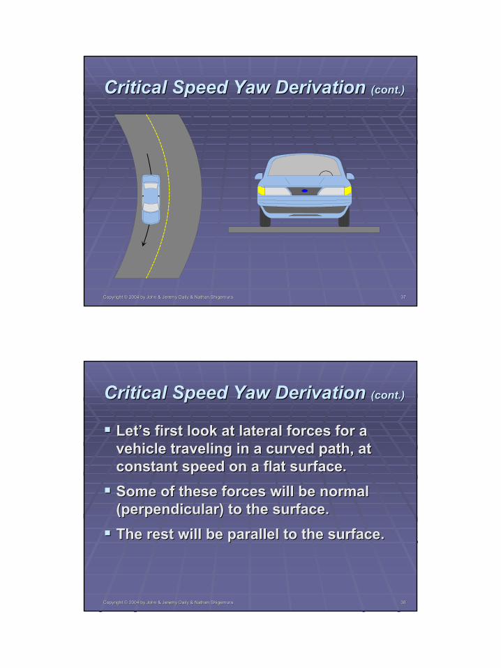
Critical Speed Yaw Derivation Critical Speed Yaw Derivation (cont.)(cont.)
Let’s first look at lateral forces for a Let’s first look at lateral forces for a vehicle traveling in a curved path, at vehicle traveling in a curved path, at constant speed on a flat surface.constant speed on a flat surface.Some of these forces will be normal Some of these forces will be normal (perpendicular) to the surface.(perpendicular) to the surface.The rest will be parallel to the surface.The rest will be parallel to the surface.

20
Copyright © 2004 by John & Jeremy Daily & Nathan ShigemuraCopyright © 2004 by John & Jeremy Daily & Nathan Shigemura 3939
Critical Speed Yaw Derivation Critical Speed Yaw Derivation (cont.)(cont.)
First, forces normal to the road surface:First, forces normal to the road surface:
W Fn
Copyright © 2004 by John & Jeremy Daily & Nathan ShigemuraCopyright © 2004 by John & Jeremy Daily & Nathan Shigemura 4040
Critical Speed Yaw Derivation Critical Speed Yaw Derivation (cont.)(cont.)
Now, let’s look at the forces parallel to Now, let’s look at the forces parallel to the roadway.the roadway.These forces will be lateral to the These forces will be lateral to the vehicle.vehicle.Some are due to the dynamics of the Some are due to the dynamics of the vehicle in the curve and some will be vehicle in the curve and some will be due to the surface friction.due to the surface friction.
21
Copyright © 2004 by John & Jeremy Daily & Nathan ShigemuraCopyright © 2004 by John & Jeremy Daily & Nathan Shigemura 4141
Critical Speed Yaw Derivation Critical Speed Yaw Derivation (cont.)(cont.)
Forces parallel to the road surface:Forces parallel to the road surface:
Ma
Ff
Copyright © 2004 by John & Jeremy Daily & Nathan ShigemuraCopyright © 2004 by John & Jeremy Daily & Nathan Shigemura 4242
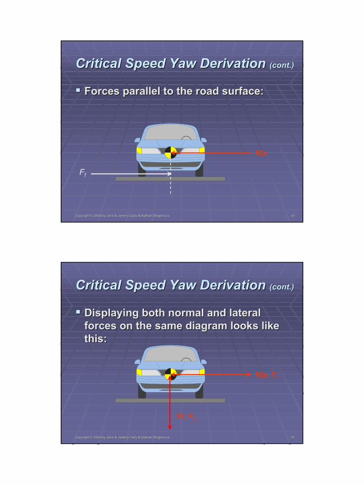
Critical Speed Yaw Derivation Critical Speed Yaw Derivation (cont.)(cont.)
Displaying both normal and lateral Displaying both normal and lateral forces on the same diagram looks like forces on the same diagram looks like this:this:
Ma, Ff
W, Fn

22
Copyright © 2004 by John & Jeremy Daily & Nathan ShigemuraCopyright © 2004 by John & Jeremy Daily & Nathan Shigemura 4343
Critical Speed Yaw Derivation Critical Speed Yaw Derivation (cont.)(cont.)
Let’s examine the lateral forces on the Let’s examine the lateral forces on the vehicle corning on a banked road.vehicle corning on a banked road.As before, there will be forces normal to As before, there will be forces normal to the road and parallel to the road.the road and parallel to the road.But we now have to take the bank, or But we now have to take the bank, or angle of the road into account.angle of the road into account.
Copyright © 2004 by John & Jeremy Daily & Nathan ShigemuraCopyright © 2004 by John & Jeremy Daily & Nathan Shigemura 4444
Critical Speed Yaw Derivation Critical Speed Yaw Derivation (cont.)(cont.)
Forces in the vertical direction:Forces in the vertical direction:
2
W
FnW cos 2
Ma
Ma sin 2
23
Copyright © 2004 by John & Jeremy Daily & Nathan ShigemuraCopyright © 2004 by John & Jeremy Daily & Nathan Shigemura 4545
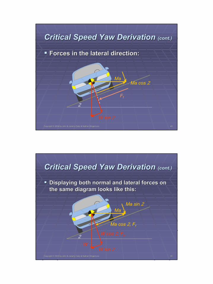
Critical Speed Yaw Derivation Critical Speed Yaw Derivation (cont.)(cont.)
Forces in the lateral direction:Forces in the lateral direction:
2
Ff
MaMa cos 2
W sin 2
Copyright © 2004 by John & Jeremy Daily & Nathan ShigemuraCopyright © 2004 by John & Jeremy Daily & Nathan Shigemura 4646
Critical Speed Yaw Derivation Critical Speed Yaw Derivation (cont.)(cont.)
Displaying both normal and lateral forces on Displaying both normal and lateral forces on the same diagram looks like this:the same diagram looks like this:
2
Ma
Ma cos 2, Ff
W sin 2
Ma sin 2
W
W cos 2, Fn
24
Copyright © 2004 by John & Jeremy Daily & Nathan ShigemuraCopyright © 2004 by John & Jeremy Daily & Nathan Shigemura 4747
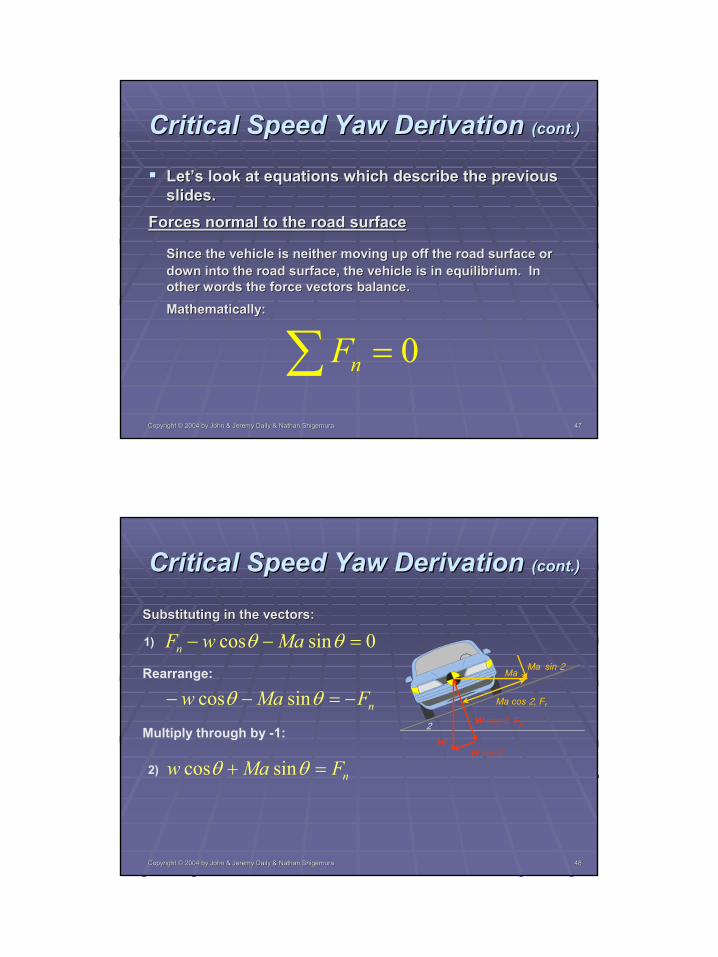
Critical Speed Yaw Derivation Critical Speed Yaw Derivation (cont.)(cont.)
Let’s look at equations which describe the previous Let’s look at equations which describe the previous slides.slides.
Forces normal to the road surfaceForces normal to the road surface
Since the vehicle is neither moving up off the road surface or Since the vehicle is neither moving up off the road surface or down into the road surface, the vehicle is in equilibrium. In down into the road surface, the vehicle is in equilibrium. In other words the force vectors balance.other words the force vectors balance.Mathematically:Mathematically:
∑ = 0nF
Copyright © 2004 by John & Jeremy Daily & Nathan ShigemuraCopyright © 2004 by John & Jeremy Daily & Nathan Shigemura 4848
Critical Speed Yaw Derivation Critical Speed Yaw Derivation (cont.)(cont.)
Substituting in the vectors:Substituting in the vectors:
2
Ma
Ma cos 2, Ff
W sin 2
Ma sin 2
W
W cos 2, Fn
0sincos =−− θθ MawFn
Rearrange:
nFMaw −=−− θθ sincos
Multiply through by -1:
nFMaw =+ θθ sincos
1)
2)

25
Copyright © 2004 by John & Jeremy Daily & Nathan ShigemuraCopyright © 2004 by John & Jeremy Daily & Nathan Shigemura 4949
Critical Speed Yaw Derivation Critical Speed Yaw Derivation (cont.)(cont.)
Forces parallel to the road surfaceForces parallel to the road surface
Since the vehicle is not sliding up or down the superelevation, Since the vehicle is not sliding up or down the superelevation, the vehicle is in equilibrium. In other words the force vectorsthe vehicle is in equilibrium. In other words the force vectorsbalance.balance.Mathematically:Mathematically:
∑ = 0tF
Copyright © 2004 by John & Jeremy Daily & Nathan ShigemuraCopyright © 2004 by John & Jeremy Daily & Nathan Shigemura 5050
Critical Speed Yaw Derivation Critical Speed Yaw Derivation (cont.)(cont.)
Substituting in the vectors:Substituting in the vectors:
2
Ma
Ma cos 2, Ff
W sin 2
Ma sin 2
W
W cos 2, Fn
0cossin =−+ θθ MawFf
Rearrange:
θθ cossin MawFf =+Recall:
nf FF µ=
3)
4)
5)
Substitute Eq. 2 into Eq. 5:
)sincos( θθµ MawFf +=6)

26
Copyright © 2004 by John & Jeremy Daily & Nathan ShigemuraCopyright © 2004 by John & Jeremy Daily & Nathan Shigemura 5151
Critical Speed Yaw Derivation Critical Speed Yaw Derivation (cont.)(cont.)
Substitute Substitute EqEq. 6 into . 6 into EqEq. 4:. 4:
θθθθµ cossin)sincos( MawMaw =++7)
8)
Expand the left side:
θθθµθµ cossinsincos MawMaw =++
Newton’s Second Law tells us that lateral acceleration is:rva
2
=
And we know:gwM =
Copyright © 2004 by John & Jeremy Daily & Nathan ShigemuraCopyright © 2004 by John & Jeremy Daily & Nathan Shigemura 5252
Critical Speed Yaw Derivation Critical Speed Yaw Derivation (cont.)(cont.)
Substitute for Substitute for MM and and aa into into EqEq. 8:. 8:
θθθµθµ cossinsincos22
rv
gww
rv
gww =++9)
Multiply both sides by and group terms:w1
10) θθθµθµ cossinsincos22
grv
grv
=++
Divide both sides by cos 2:
grv
grv 22
cossin
cossin
=++θθ
θθµµ11)
27
Copyright © 2004 by John & Jeremy Daily & Nathan ShigemuraCopyright © 2004 by John & Jeremy Daily & Nathan Shigemura 5353
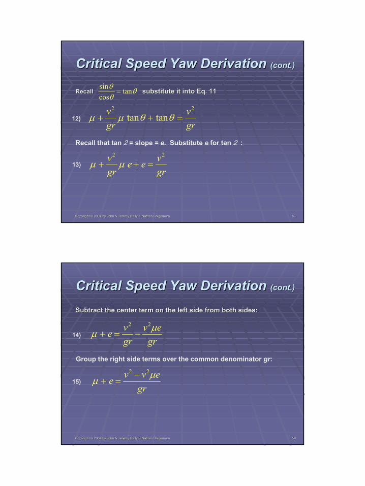
Critical Speed Yaw Derivation Critical Speed Yaw Derivation (cont.)(cont.)
Recall Recall substitute it into substitute it into EqEq. 11. 11θθθ tan
cossin
=
12)grv
grv 22
tantan =++ θθµµ
Recall that tan 2 = slope = e. Substitute e for tan 2 :
13)grvee
grv 22
=++ µµ
Copyright © 2004 by John & Jeremy Daily & Nathan ShigemuraCopyright © 2004 by John & Jeremy Daily & Nathan Shigemura 5454
Critical Speed Yaw Derivation Critical Speed Yaw Derivation (cont.)(cont.)
Subtract the center term on the left side from both sides:Subtract the center term on the left side from both sides:
14)gr
evgrve µµ
22
−=+
Group the right side terms over the common denominator gr:
15)gr
evve µµ22 −
=+
28
Copyright © 2004 by John & Jeremy Daily & Nathan ShigemuraCopyright © 2004 by John & Jeremy Daily & Nathan Shigemura 5555
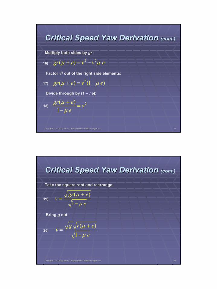
Critical Speed Yaw Derivation Critical Speed Yaw Derivation (cont.)(cont.)
Multiply both sides by Multiply both sides by grgr ::
evvegr µµ 22)( −=+16)
17)
Factor v2 out of the right side elements:
)1()( 2 evegr µµ −=+
Divide through by (1 – :e):
18) 2
1)( v
eegr=
−+µµ
Copyright © 2004 by John & Jeremy Daily & Nathan ShigemuraCopyright © 2004 by John & Jeremy Daily & Nathan Shigemura 5656
Critical Speed Yaw Derivation Critical Speed Yaw Derivation (cont.)(cont.)
Take the square root and rearrange:Take the square root and rearrange:
19)eegr
vµµ−
+=
1)(
Bring g out:
20)e
ergv
µµ
−
+=
1)(
29
Copyright © 2004 by John & Jeremy Daily & Nathan ShigemuraCopyright © 2004 by John & Jeremy Daily & Nathan Shigemura 5757
Critical Speed Yaw Derivation Critical Speed Yaw Derivation (cont.)(cont.)
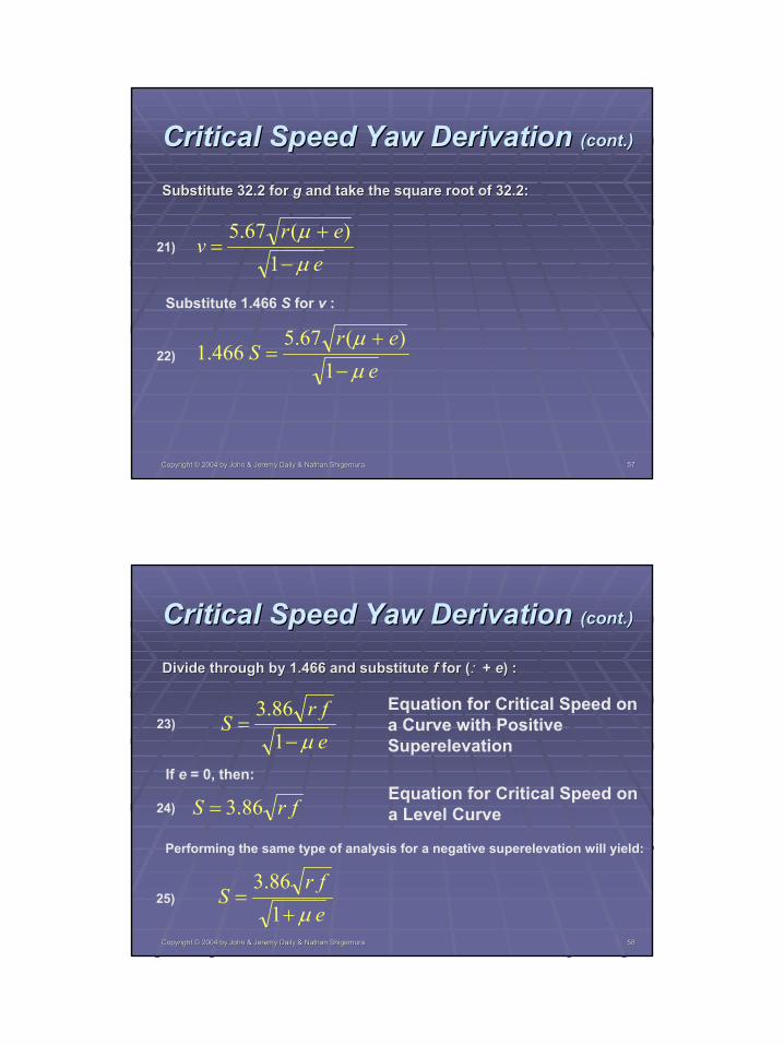
Substitute 32.2 for Substitute 32.2 for gg and take the square root of 32.2:and take the square root of 32.2:
Substitute 1.466 S for v :
eer
vµµ
−
+=
1)(67.5
21)
22)e
erS
µµ
−
+=
1)(67.5
466.1
Copyright © 2004 by John & Jeremy Daily & Nathan ShigemuraCopyright © 2004 by John & Jeremy Daily & Nathan Shigemura 5858
Critical Speed Yaw Derivation Critical Speed Yaw Derivation (cont.)(cont.)
Divide through by 1.466 and substitute Divide through by 1.466 and substitute ff for (for (:: + + ee) :) :
23)efr
Sµ−
=186.3 Equation for Critical Speed on
a Curve with Positive Superelevation
24) frS 86.3=
If e = 0, then:Equation for Critical Speed on a Level Curve
Performing the same type of analysis for a negative superelevation will yield:
efr
Sµ+
=186.3
25)
30
9/26/2004©John Daily, Nathan Shigemura, Jeremy DailyPage 59
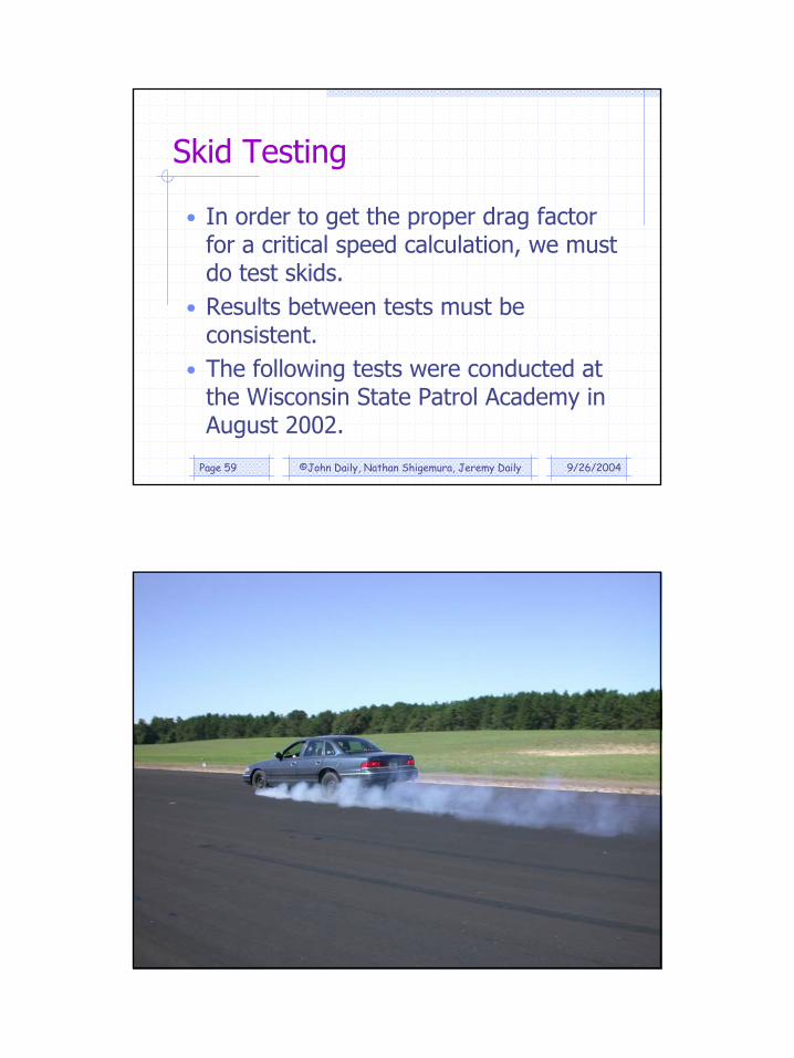
Skid Testing
• In order to get the proper drag factor for a critical speed calculation, we must do test skids.
• Results between tests must be consistent.
• The following tests were conducted at the Wisconsin State Patrol Academy in August 2002.
9/26/2004©John Daily, Nathan Shigemura, Jeremy DailyPage 60
31
9/26/2004©John Daily, Nathan Shigemura, Jeremy DailyPage 61
9/26/2004©John Daily, Nathan Shigemura, Jeremy DailyPage 62
32
9/26/2004©John Daily, Nathan Shigemura, Jeremy DailyPage 63
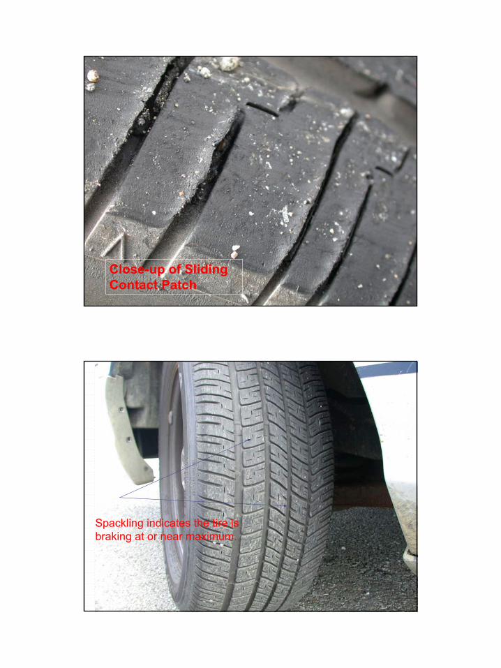
Close-up of Sliding Contact Patch
9/26/2004©John Daily, Nathan Shigemura, Jeremy DailyPage 64
Spackling indicates the tire is braking at or near maximum.
33
9/26/2004©John Daily, Nathan Shigemura, Jeremy DailyPage 65
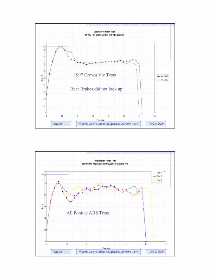
Deceleration Factor Testsfor 1997 Ford Crown Victoria with ABS Disabled
0
0.1
0.2
0.3
0.4
0.5
0.6
0.7
0.8
0.9
1
0 0.5 1 1.5 2 2.5 3 3.5
Time (sec)
G o
r f w /o ABS(1)
w /o ABS(2)
1997 Crown Vic Tests
Rear Brakes did not lock up
9/26/2004©John Daily, Nathan Shigemura, Jeremy DailyPage 66
Deceleration Factor Testsfrom VC2000 Accelerometer for 2002 Pontiac Grand Prix
0
0.2
0.4
0.6
0.8
1
1.2
0 0.5 1 1.5 2 2.5 3
Time (sec)
G o
r f
Trial 1Trial 2Trial 3
All Pontiac ABS Tests

34
9/26/2004©John Daily, Nathan Shigemura, Jeremy DailyPage 67
Acceleration Factor Testsfrom VC2000 Accelerometer
0
0.2
0.4
0.6
0.8
1
1.2
0 0.5 1 1.5 2 2.5 3 3.5 4 4.5 5
Time (sec)
G o
r f
Trial 1
Trial 2
Trial 3
w / ABS
w /o ABS(1)
w /o ABS(2)
hi speed
All Test Skids
9/26/2004©John Daily, Nathan Shigemura, Jeremy DailyPage 68
Measuring Grade
35
9/26/2004©John Daily, Nathan Shigemura, Jeremy DailyPage 69
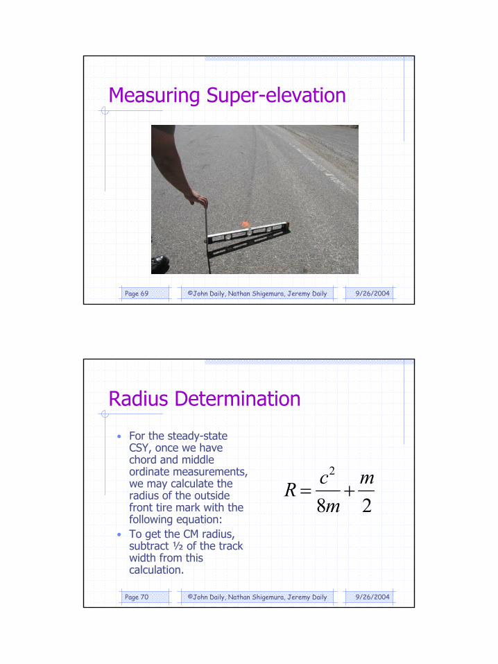
Measuring Super-elevation
9/26/2004©John Daily, Nathan Shigemura, Jeremy DailyPage 70
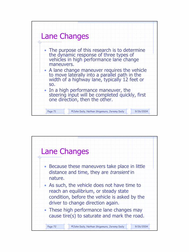
Radius Determination
• For the steady-state CSY, once we have chord and middle ordinate measurements, we may calculate the radius of the outside front tire mark with the following equation:
• To get the CM radius, subtract ½ of the track width from this calculation.
28
2 mm
cR +=
36
9/26/2004©John Daily, Nathan Shigemura, Jeremy DailyPage 71
Lane Changes
• The purpose of this research is to determine the dynamic response of three types of vehicles in high performance lane change maneuvers.
• A lane change maneuver requires the vehicle to move laterally into a parallel path in the width of a highway lane, typically 12 feet or so.
• In a high performance maneuver, the steering input will be completed quickly, first one direction, then the other.
9/26/2004©John Daily, Nathan Shigemura, Jeremy DailyPage 72
Lane Changes
• Because these maneuvers take place in little distance and time, they are transient in nature.
• As such, the vehicle does not have time to reach an equilibrium, or steady state condition, before the vehicle is asked by the driver to change direction again.
• These high performance lane changes may cause tire(s) to saturate and mark the road.
37
9/26/2004©John Daily, Nathan Shigemura, Jeremy DailyPage 73
Lane Changes
• To a neophyte investigator, these tire marks may sometimes be mistaken for CSY marks.
• Because of the transient nature of the vehicle motion, we may not use a classical CSY analysis to compute speed from these marks.
• We will design testing to examine important aspects of vehicle motion during lane change maneuvers.
• We will also examine the potential error of using a CSY analysis for speed, and will examine the sources of the error.
9/26/2004©John Daily, Nathan Shigemura, Jeremy DailyPage 74
Lane Changes
• Simple models exist to generally examine lane change maneuvers if the entrance speed and lateral acceleration are specified. (FTAR Chapter 7)
• These models were initially developed to examine lane changes with lateral accelerations encountered in normal driving.
• The distance equation of the analysis was essentially validated in SAE 2002-01-0817 (Araszewski, et al).
• The average error for 15 tests was 0%.
38
9/26/2004©John Daily, Nathan Shigemura, Jeremy DailyPage 75
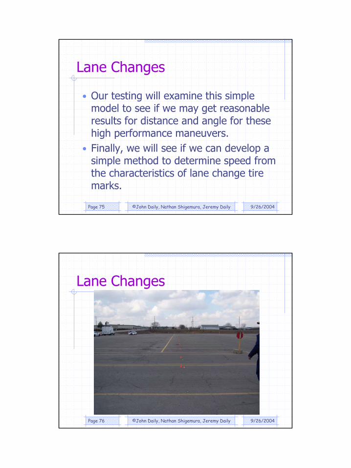
Lane Changes
• Our testing will examine this simple model to see if we may get reasonable results for distance and angle for these high performance maneuvers.
• Finally, we will see if we can develop a simple method to determine speed from the characteristics of lane change tire marks.
9/26/2004©John Daily, Nathan Shigemura, Jeremy DailyPage 76
Lane Changes
39
9/26/2004©John Daily, Nathan Shigemura, Jeremy DailyPage 77
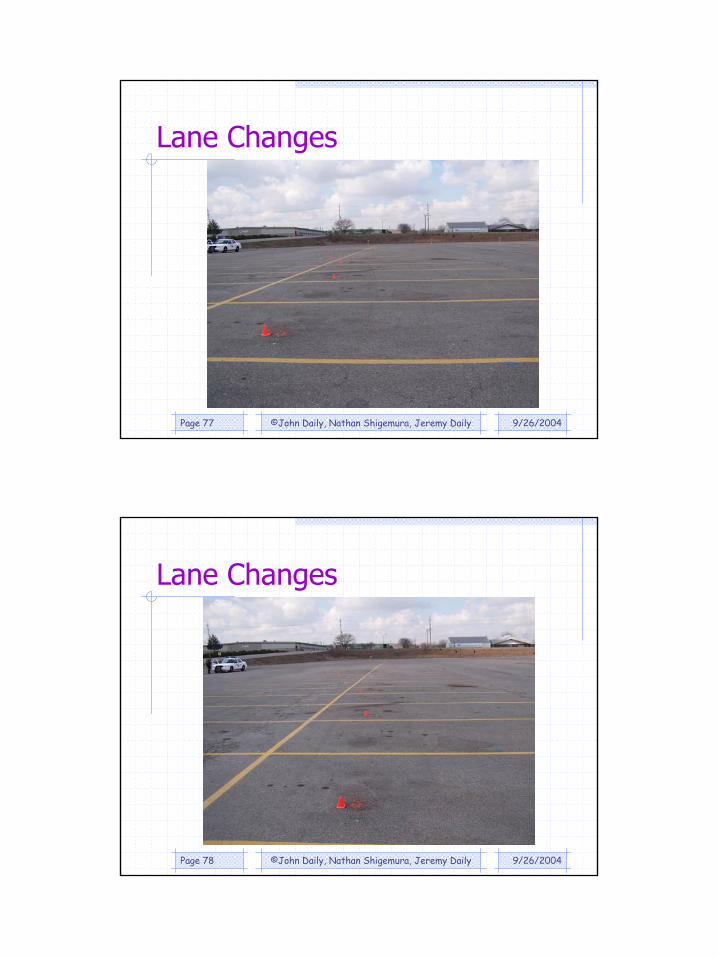
Lane Changes
9/26/2004©John Daily, Nathan Shigemura, Jeremy DailyPage 78
Lane Changes
40
9/26/2004©John Daily, Nathan Shigemura, Jeremy DailyPage 79
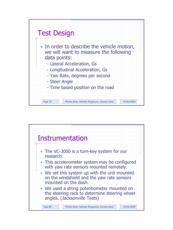
Test Design
• In order to describe the vehicle motion, we will want to measure the following data points:– Lateral Acceleration, Gs– Longitudinal Acceleration, Gs– Yaw Rate, degrees per second– Steer Angle– Time based position on the road
9/26/2004©John Daily, Nathan Shigemura, Jeremy DailyPage 80
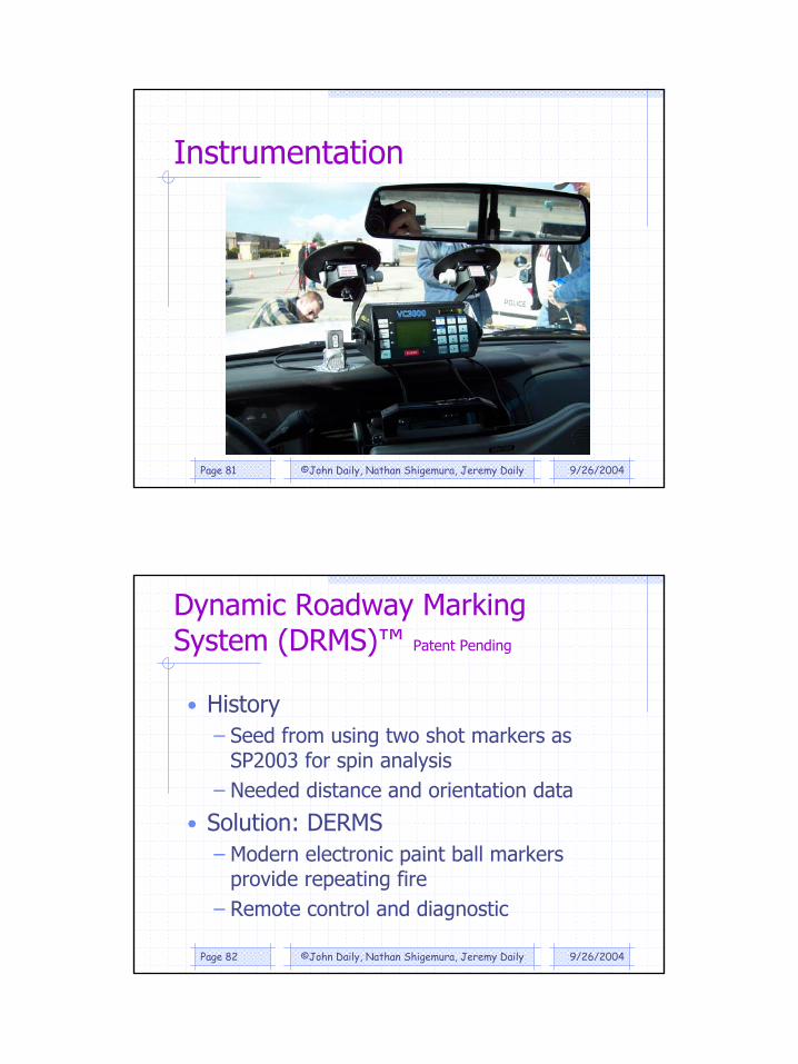
Instrumentation
• The VC-3000 is a turn-key system for our research.
• This accelerometer system may be configured with yaw rate sensors mounted remotely.
• We set this system up with the unit mounted on the windshield and the yaw rate sensors mounted on the dash.
• We used a string potentiometer mounted on the steering rack to determine steering wheel angles. (Jacksonville Tests)
41
9/26/2004©John Daily, Nathan Shigemura, Jeremy DailyPage 81
Instrumentation
9/26/2004©John Daily, Nathan Shigemura, Jeremy DailyPage 82
Dynamic Roadway Marking System (DRMS)™ Patent Pending
• History– Seed from using two shot markers as
SP2003 for spin analysis– Needed distance and orientation data
• Solution: DERMS– Modern electronic paint ball markers
provide repeating fire– Remote control and diagnostic
42
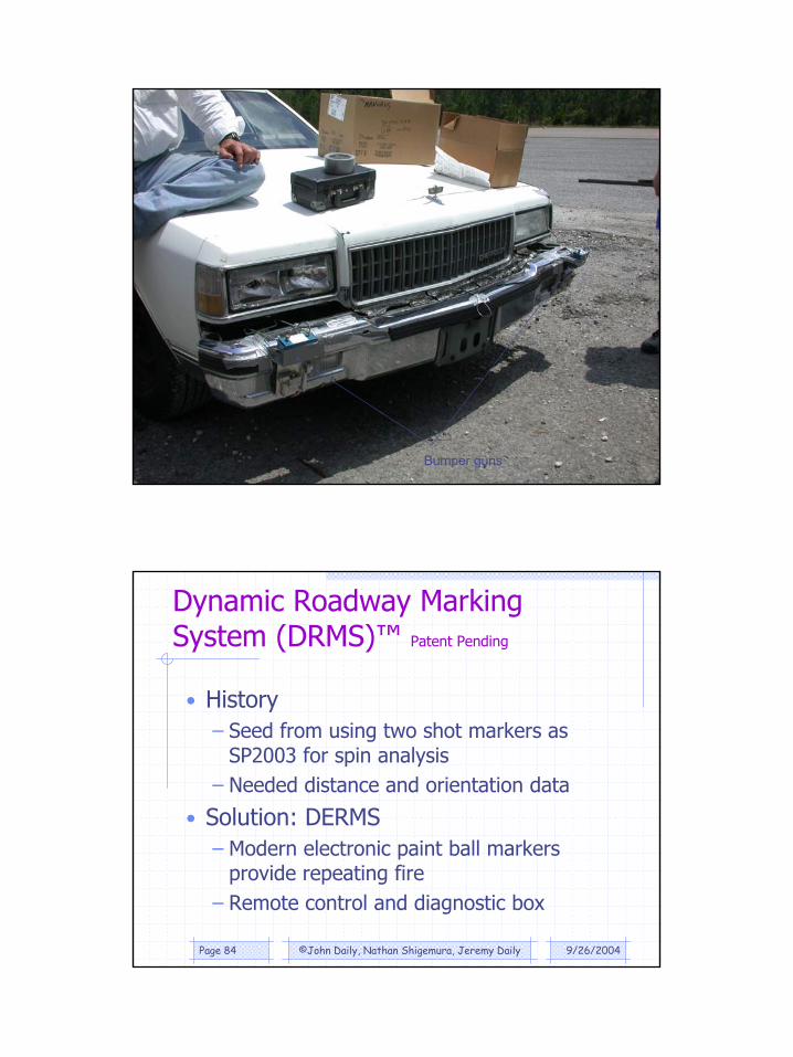
9/26/2004©John Daily, Nathan Shigemura, Jeremy DailyPage 83 Bumper guns
9/26/2004©John Daily, Nathan Shigemura, Jeremy DailyPage 84
Dynamic Roadway Marking System (DRMS)™ Patent Pending
• History– Seed from using two shot markers as
SP2003 for spin analysis– Needed distance and orientation data
• Solution: DERMS– Modern electronic paint ball markers
provide repeating fire– Remote control and diagnostic box

43
9/26/2004©John Daily, Nathan Shigemura, Jeremy DailyPage 85
DRMS Mounted to the Receiver on a Dodge Dakota
9/26/2004©John Daily, Nathan Shigemura, Jeremy DailyPage 86
DRMS Mounted to the License Plate Bracket of the Dakota

44
9/26/2004©John Daily, Nathan Shigemura, Jeremy DailyPage 87
DRMS Mounted on the Back of a Ford Crown Victoria
9/26/2004©John Daily, Nathan Shigemura, Jeremy DailyPage 88
Dodge Dakota (Ohio Testing)
Center of Mass
WRear WFront
Length
Midpoint
45
9/26/2004©John Daily, Nathan Shigemura, Jeremy DailyPage 89
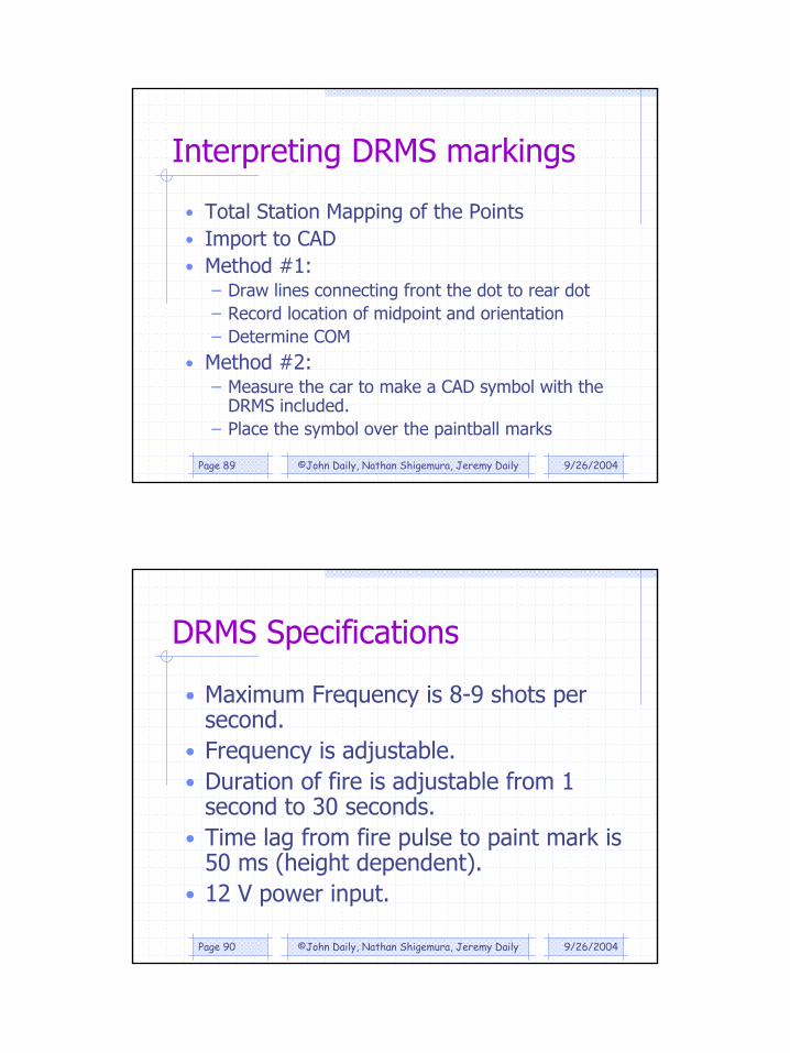
Interpreting DRMS markings
• Total Station Mapping of the Points• Import to CAD• Method #1:
– Draw lines connecting front the dot to rear dot– Record location of midpoint and orientation– Determine COM
• Method #2:– Measure the car to make a CAD symbol with the
DRMS included.– Place the symbol over the paintball marks
9/26/2004©John Daily, Nathan Shigemura, Jeremy DailyPage 90
DRMS Specifications
• Maximum Frequency is 8-9 shots per second.
• Frequency is adjustable.• Duration of fire is adjustable from 1
second to 30 seconds.• Time lag from fire pulse to paint mark is
50 ms (height dependent).• 12 V power input.

46
9/26/2004©John Daily, Nathan Shigemura, Jeremy DailyPage 91
DRMS Features
• Remote firing of markers.• Communicates with the VC3000.• Provides a physical link between roadway
evidence and instrument data• Usable on any vehicle
– Mounts to a license plate bracket– Mounts to a hitch receiver– Drill new mounting points
• Consistent time base between shots
9/26/2004©John Daily, Nathan Shigemura, Jeremy DailyPage 92
Information Provided by DRMS
• Time when markers are fired• If one marker:
– Location of one point of car– Orientation and Center of Mass location if there
are tire marks
• If two markers:– Location and orientation regardless of tire
evidence
• Speed and acceleration can be backed out
47
9/26/2004©John Daily, Nathan Shigemura, Jeremy DailyPage 93
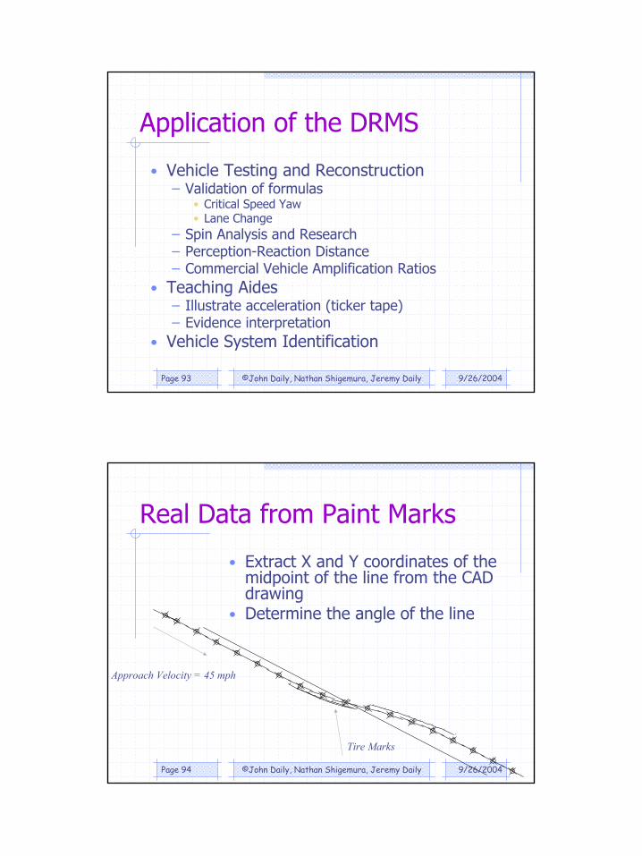
Application of the DRMS
• Vehicle Testing and Reconstruction – Validation of formulas
• Critical Speed Yaw• Lane Change
– Spin Analysis and Research– Perception-Reaction Distance– Commercial Vehicle Amplification Ratios
• Teaching Aides– Illustrate acceleration (ticker tape)– Evidence interpretation
• Vehicle System Identification
9/26/2004©John Daily, Nathan Shigemura, Jeremy DailyPage 94
7
Line
Line1
Line2
Line
Line
Line
Line
Line
Line
Line
Line2
Line2
Line1
Line2
Line1
Line2
Line1
Line2
Line1
Line2
Line1
Line2
1
4
3
5
6
8
9
10
11
12
13
14
15
16
17
18
2
Real Data from Paint Marks
• Extract X and Y coordinates of the midpoint of the line from the CAD drawing
• Determine the angle of the line
Approach Velocity = 45 mph
Tire Marks
48
9/26/2004©John Daily, Nathan Shigemura, Jeremy DailyPage 95
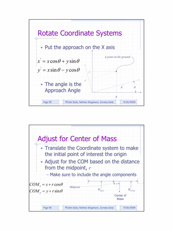
Rotate Coordinate Systems
• Put the approach on the X axis
• The angle is the Approach Angle
θθ
θθ
cossinsincos
'
'
yxyyxx
−=
+=
x
y
y’
x’ θ
A point on the ground
9/26/2004©John Daily, Nathan Shigemura, Jeremy DailyPage 96
Adjust for Center of Mass• Translate the Coordinate system to make
the initial point of interest the origin• Adjust for the COM based on the distance
from the midpoint, r– Make sure to include the angle components
r
Center of Mass
WRear WFront
Midpointθθ
sincos
ryCOMrxCOM
y
x
+=+=
49
9/26/2004©John Daily, Nathan Shigemura, Jeremy DailyPage 97
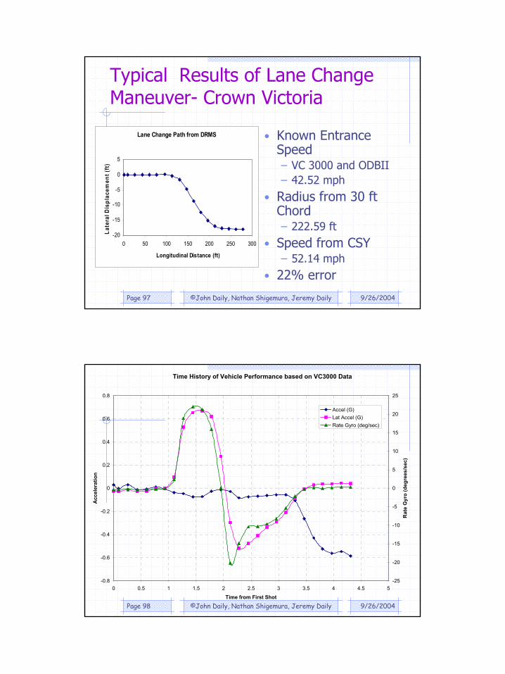
Typical Results of Lane Change Maneuver- Crown Victoria
Lane Change Path from DRMS
-20
-15
-10
-5
0
5
0 50 100 150 200 250 300
Longitudinal Distance (ft)
Late
ral D
ispl
acem
ent (
ft)
• Known Entrance Speed – VC 3000 and ODBII– 42.52 mph
• Radius from 30 ft Chord– 222.59 ft
• Speed from CSY– 52.14 mph
• 22% error
9/26/2004©John Daily, Nathan Shigemura, Jeremy DailyPage 98
Time History of Vehicle Performance based on VC3000 Data
-0.8
-0.6
-0.4
-0.2
0
0.2
0.4
0.6
0.8
0 0.5 1 1.5 2 2.5 3 3.5 4 4.5 5
Time from First Shot
Acc
eler
atio
n
-25
-20
-15
-10
-5
0
5
10
15
20
25
Rat
e G
yro
(deg
rees
/sec
)Accel (G)Lat Accel (G)Rate Gyro (deg/sec)
50
9/26/2004©John Daily, Nathan Shigemura, Jeremy DailyPage 99
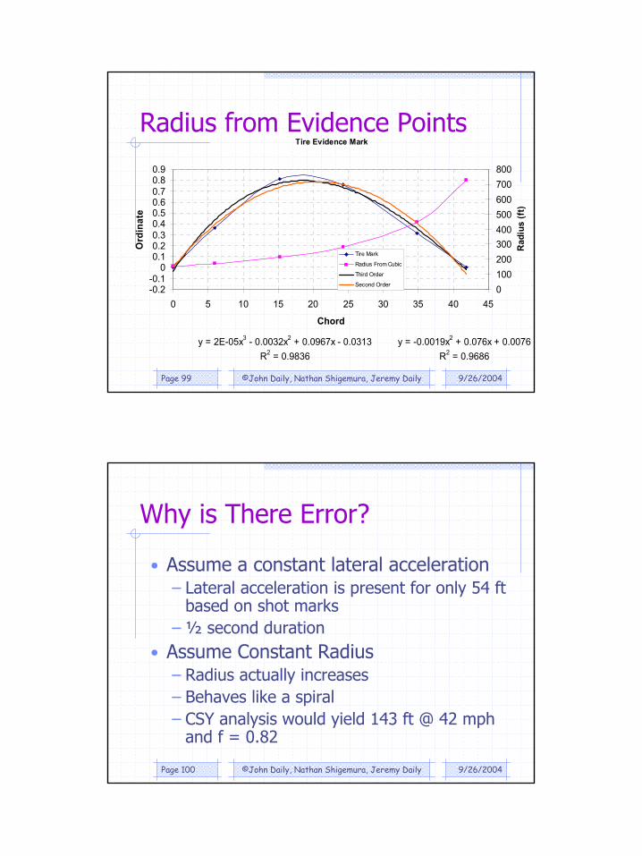
Tire Evidence Mark
y = 2E-05x3 - 0.0032x2 + 0.0967x - 0.0313R2 = 0.9836
y = -0.0019x2 + 0.076x + 0.0076R2 = 0.9686
-0.2-0.1
00.10.20.30.40.50.60.70.80.9
0 5 10 15 20 25 30 35 40 45
Chord
Ord
inat
e
0100200300400500600700800
Rad
ius
(ft)
Tire Mark
Radius From Cubic
Third Order
Second Order
Radius from Evidence Points
9/26/2004©John Daily, Nathan Shigemura, Jeremy DailyPage 100
Why is There Error?
• Assume a constant lateral acceleration– Lateral acceleration is present for only 54 ft
based on shot marks– ½ second duration
• Assume Constant Radius– Radius actually increases– Behaves like a spiral– CSY analysis would yield 143 ft @ 42 mph
and f = 0.82
51
9/26/2004©John Daily, Nathan Shigemura, Jeremy DailyPage 101
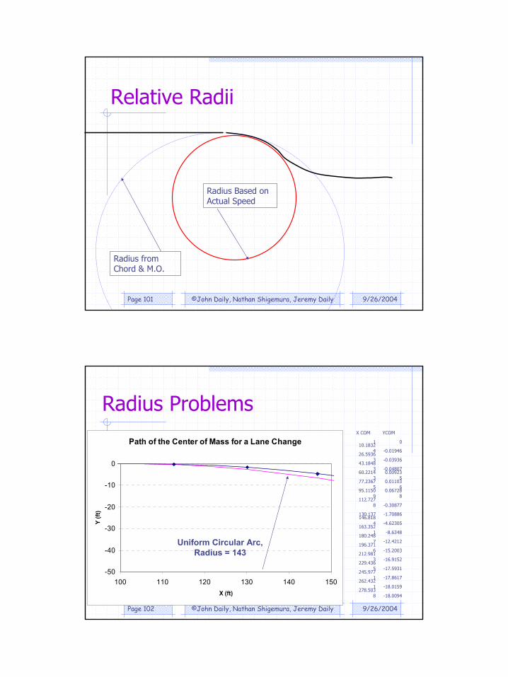
Relative Radii
Radius from Chord & M.O.
Radius Based on Actual Speed
9/26/2004©John Daily, Nathan Shigemura, Jeremy DailyPage 102
Path of the Center of Mass for a Lane Change
-50
-40
-30
-20
-10
0
100 110 120 130 140 150X (ft)
Y (ft
)
Radius Problems
-18.0094278.503
8
-18.0159262.432
1
-17.8617245.977
1
-17.5931229.436
5
-16.9152212.981
3
-15.2003196.371
6
-12.4212180.248
7
-8.6348163.352
1
-4.62305146.818
4
-1.70886130.137
-0.30877112.727
8
0.067288
95.11509
0.011036
77.23675
0.009235
60.22143
-0.0480743.1848
3
-0.0393626.5936
3
-0.0194610.1832
4
01
YCOMX COM
Uniform Circular Arc, Radius = 143

52
9/26/2004©John Daily, Nathan Shigemura, Jeremy DailyPage 103
Lane Change Maneuver for a Dodge Dakota
• Known Entrance Speed – VC 3000 – 43.34 mph
• Radius from 30 ft Chord– 232.54 ft
• Speed from CSY– 51.98 mph
• 19.9% error
Lane Change Path from DRMS
-20
-18
-16
-14
-12
-10
-8
-6
-4
-2
0
2
0 50 100 150 200 250
Longitudinal Distance (ft)
Late
ral D
ispl
acem
ent (
ft)
9/26/2004©John Daily, Nathan Shigemura, Jeremy DailyPage 104
Lane Change Example of a Pickup Time History of Vehicle Performance based on VC3000 Data
-0.6
-0.4
-0.2
0
0.2
0.4
0.6
0.8
0 0.5 1 1.5 2 2.5 3 3.5 4 4.5
Time from First Shot
Acc
eler
atio
n
-20
-15
-10
-5
0
5
10
15
20
25
Rat
e G
yro
(deg
rees
/sec
)
Accel (G)Lat Accel (G)Rate Gyro (deg/sec)
53
9/26/2004©John Daily, Nathan Shigemura, Jeremy DailyPage 105
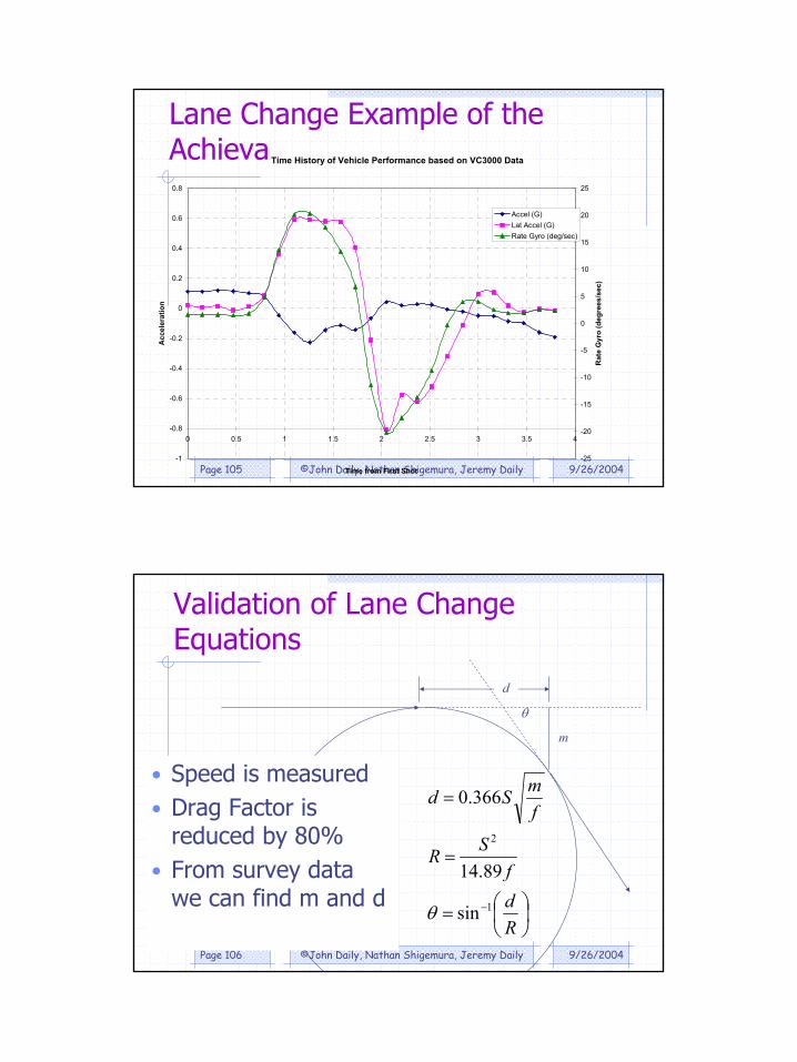
Lane Change Example of the Achieva Time History of Vehicle Performance based on VC3000 Data
-1
-0.8
-0.6
-0.4
-0.2
0
0.2
0.4
0.6
0.8
0 0.5 1 1.5 2 2.5 3 3.5 4
Time from First Shot
Acc
eler
atio
n
-25
-20
-15
-10
-5
0
5
10
15
20
25
Rat
e G
yro
(deg
rees
/sec
)
Accel (G)Lat Accel (G)Rate Gyro (deg/sec)
9/26/2004©John Daily, Nathan Shigemura, Jeremy DailyPage 106
Validation of Lane Change Equations
=
=
=
−
Rdf
SR
fmSd
1
2
sin
89.14
366.0
θ
d
m
θ
• Speed is measured• Drag Factor is
reduced by 80%• From survey data
we can find m and d
54
9/26/2004©John Daily, Nathan Shigemura, Jeremy DailyPage 107
Validation of Lane Change Equations
• Predicted angle agrees with measured angle within 2 degrees
• Distance agrees within 2 feet• Computes an “Effective Radius”• Working backward to obtain speed is
too sensitive to the small angle. • 2 degrees can give 10 mph differences.
9/26/2004©John Daily, Nathan Shigemura, Jeremy DailyPage 108
Speed From Lane Change
• Work in this area is preliminary, but shows promise.
• We wish to develop techniques that will allow the scene investigator to take evidence measurements that may be converted into a path radius that is both accurate and repeatable.
• We must also account for the shape of the lateral acceleration curve.
55
9/26/2004©John Daily, Nathan Shigemura, Jeremy DailyPage 109
Speed From Lane Change
Work with the Olds tests in Jacksonville have resulted in a speed calculation within one mph of the integrated entry speed.
More analysis and more tests need to be done, but the method shows promise and will be published when finished.
9/26/2004©John Daily, Nathan Shigemura, Jeremy DailyPage 110
Summary and Conclusions
• CSY Analysis is inappropriate for determining speed from a transient lane change maneuver.
• Interpretation of the evidence is paramount to recognizing the lane change.
• Testing was conducted using the VC3000DAQ Accelerometer and the Dynamic Roadway Marking System™
• Test show errors for lane changes• Lane Change equations presented in FTAR
are validated.