a study on dem-derived primary topographic attributes for...

ARTICLE IN PRESS

0143-6228/$ - se

doi:10.1016/j.ap

�CorrespondE-mail addr

Applied Geography 28 (2008) 210–223

www.elsevier.com/locate/apgeog

A study on DEM-derived primary topographic attributes forhydrologic applications: Sensitivity to elevation data resolution

Simon Wua,�, Jonathan Lib, G.H. Huangc

aEnvironmental Systems Engineering, University of Regina, Box 413, 4246 Albert Street, Regina, Saskatchewan, Canada S4S 3R9bDepartment of Geography, University of Waterloo, Waterloo, Ontario, Canada N2L 3G1

cDepartment of Civil & Environmental Engineering, University of Waterloo, Waterloo, Ontario, Canada N2L 3G1

Abstract

Primary topographic attributes play a critical role in determining watershed hydrologic characteristics for water

resources modeling with raster-based digital elevation models (DEM). The effects of DEM resolution on a set of important

topographic derivatives are examined in this study, including slope, upslope contributing area, flow length and watershed

area. The focus of the study is on how sensitive each of the attributes is to the resolution uncertainty by considering the

effects of overall terrain gradient and bias from resampling. Two case study watersheds of different gradient patterns are

used with their 10m USGS DEMs. A series of DEMs up to 200m grid size are produced from the base DEMs using three

commonly used resampling methods. All the terrain variables tested vary with the grid size change. It is found that slope

angles decrease and contributing area values increase constantly as DEMs are aggregated progressively to coarser

resolutions. No systematic trend is observed for corresponding changes of flow path and watershed area. The analysis also

suggests that gradient profile of the watershed presents an important factor for the examined sensitivities to DEM

resolution.

r 2008 Elsevier Ltd. All rights reserved.

Keywords: Digital elevation model; Grid size; Topographic attributes; Hydrologic modeling

Introduction

Topography defines the pathways of surface water movement across a watershed, and thus is a major factoraffecting watershed hydrologic response to rainfall inputs. Raster-based digital elevation models (DEMs) havebeen widely applied to efficiently derive topographic attributes used in hydrologic modeling such as slope andupslope contributing area. Any uncertainties in the topographic models will be propagated into the output ofhydrologic model prediction, causing inaccuracies. One of such uncertainties stems from the choice of DEMgrid size.

The availability of digital elevation data has been greatly increased with the development of effective spatialdata acquisition tools (Huang & Chang, 2003). DEM accuracy properties including grid size could, however,

e front matter r 2008 Elsevier Ltd. All rights reserved.

geog.2008.02.006

ing author.

ess: [email protected] (S. Wu).

www.elsevier.com/locate/apgeog

dx.doi.org/10.1016/j.apgeog.2008.02.006

mailto:[email protected]

ARTICLE IN PRESSS. Wu et al. / Applied Geography 28 (2008) 210–223 211

vary from source to source for an area of interest. The sensitivity of principal topographic derivatives used inhydrologic modeling to DEM resolution, however, has been systematically explored in few studies. A numberof studies have shown that lower resolution DEMs under-represent slope classes (Bolstad & Stowe, 1994;Chang & Tsai, 1991; Gao, 1997; Kienzle, 2004; Thompson, Bell, & Butler, 2001; Zhang, Drake, Wainwright,& Mulligan, 1999). Zhang and Montgomery (1994) examined the effect of grid cell resolution on landscaperepresentation and hydrologic simulations using elevation data from two small watersheds. Their resultsshowed that increasing the grid size resulted in an increased mean topographic index because of increasedcontributing area and decreased slopes. Another study on DEM resolution effect on surface runoff modelingby Vieux (1993) showed that aggregation of spatial input data led to a decrease in the flow path length of themain channel. The result was believed to be attributable to the short circuiting of meanders in the originalDEM. The same work also showed that the watershed area varies with increasing DEM grid size without aconsistent trend.

Wilson and Gallant (2000) provided a summary on topographic properties where direct surface derivativesfrom DEM are categorized as primary topographic attributes. Among the primary attributes, those of mostinterest to hydrologists in terms of DEM resolution effect include slope, flow length, upslope contributingarea, and watershed area. This work examines DEM resolution uncertainty in watershed terrainrepresentation with the four important variables.

Flow path determination serves as the basis for extracting drainage networks and watershed delineationfrom DEMs in hydrologic modeling. Slope is a fundamental topographic property used in all flow pathalgorithms. Slope, together with aspect, determines the flow direction from which the upslope contributingarea, representing the accumulated area draining into a given grid cell can be calculated. The calculation of theupslope contributing area is a cell-by-cell operation, and stream networks and watershed boundaries can beidentified from its results across the DEM. Slope and upslope contributing area determine the topographicindex which is popularly used in water resources applications. The index is defined as the natural logarithm ofthe ratio of the upslope contributing area to the ground surface slope. It has been the core element in varioushydrologic models such as TOPMODEL (Beven & Kirkby, 1979) where it represents the extension ofsaturated areas and the spatial variation of soil moisture and groundwater levels.

Flow length is a measure of the distance along the flow path (determined by the flow direction grid) from agiven cell to its drainage basin outlet. Variations with flow length may lead to significant change to the time lagbetween precipitation and flow peak discharge, thus resulting in a much different hydrograph. The sensitivityof watershed area to DEM resolution also deserves an examination. The rainfall coverage used to obtainrainfall input to the model must be corresponding to the watershed area determined from the applied DEM.Watershed area could also be an important factor in many hydrologic model’s calibration processes as it isused in calculating unit runoff volumes. Optimized model parameters may be affected by any discrepancybetween the area used in observed runoff and that for modeling prediction.

The comparative approach using different grid sizes of DEM has been commonly used for examining theeffect of spatial data resolution on hydrologic models and their parameters (Saulnier, Beven, & Obled, 1997;Vieux, 1993; Wolock & Price, 1994; Wu, Li, & Huang, 2007; Zhang & Montgomery, 1994). Sensitivity profilescan be seen straightforwardly by depicting the variation of modeling results with DEM grid size. However,multiple resolutions of DEM suitable for the study are often not readily available for an area of interest. Mostof the studies have used grid cell aggregation, i.e., resampling a given DEM to coarser resolutions, to explorethe effect of cell size selection. In DEM resampling, the values of output cells are obtained by interpolationbased on the values of input cells combined with the calculated distortion. Quite some resampling techniquesexist, but only a few of them have been widely used in DEM grid cell aggregation. Multiple techniques areselected and applied in this study to see whether any significant inconsistency can be brought into modelingresults by different resampling methods, ensuring that the cell aggregation approach is appropriate for thecomparative study.

Study areas

The case study areas used in this study are two small catchments located inside Back Creek Watershed inSouthwest Virginia. The two catchments (signified as A and B hereafter) occupy areas of 2.83 and 4.71 km2,

ARTICLE IN PRESS

Fig. 1. DEM maps for the two study watersheds.

S. Wu et al. / Applied Geography 28 (2008) 210–223212

respectively. Catchment A lies in a low-relief landscape close to the watershed outlet, and its surface elevationranges from 250 to 337m. Catchment B is situated upstream of the watershed, and its overall terrain presentsdistinct variability with elevation varying from 395 to 971m. The digital elevation quadrangles at 10mresolution containing the study areas were downloaded from the data center website of the United StatesGeological Survey (USGS). The catchments are delineated and extracted with the Hydrology Tools of ESRIArcGIS Spatial Analyst (Fig. 1).

Methods

Resampling

The three most commonly used resampling techniques are applied in this study. They are nearest-neighborinterpolation, bilinear interpolation and cubic convolution (Keys, 1981; Mitchell & Netravali, 1988). Thenearest-neighbor method simply assigns the value of the single closest observation to each cell. Once thelocation of the cell’s center on the output grid is located on the input DEM, the nearest neighbor assignmentwill determine the location of the closest cell center on the input grid, identify the value that is associated withthe cell, and assign that value to the cell that the output cell center is associated with. The bilinearinterpolation takes a weighted average of the nearest four input cells around the transformed point todetermine the output cell. This method results in a smoother surface than the nearest-neighbor method. In thecubic convolution technique, the output cell value is computed by fitting a smooth surface to the nearest 16input cells. It tends to smooth data even more than the bilinear interpolation.

The 10m DEM of each of the two catchments is used as the base resolution, and resampled to five DEMs of30, 60, 90, 150, and 200m resolutions using each of the three resampling methods, respectively.


Sink filling

A common problem with drainage network delineation using DEM is the presence of sinks. A DEM sinkoccurs when all neighboring cells are higher than the processing cell, which has no downslope flow path to aneighbor cell. Sinks could be real components of the terrain, but are also the results of input errors orinterpolation artifacts produced in DEM generation or resampling process. They cause obstacles to thecalculation of flow direction, leading to inaccurate representation of flow accumulation, and thus drainagenetworks. Therefore the sinks are commonly removed prior to DEM processing for drainage identification. Inthis study, the target attributes should be derived from hydrologically sound elevation data, i.e., sink-freeDEMs. There have been a number of methods developed for treating sinks in DEMs (Garbrecht & Martz,1999). A straightforward technique is to fill the sinks by increasing the values of cells in each sink by the valueof the cell with the lowest value on the sink’s boundary (Band, 1986; Jenson & Domingue, 1988; O’Callaghan& Mark, 1984). The sink filling using this approach is performed in this study on each DEM before thecalculation of the topographic attributes.

Calculation of topographic attributes

The four topographic derivatives are generated with the base DEM and all the resampled DEMs using eachof the three resampling techniques. Slope calculation is performed on the DEM using a 3� 3 cellneighborhood in most commonly used algorithms. The method of Horn (1981) is adopted in this study. Themethod is one of eight algorithms examined comparatively in a study by Jones (1998) using both synthetic andreal data as test surface. The study showed that Horn’s method performed well for gradient estimation basedon root-mean-square (RMS) residual error estimates. Unequal weighting coefficients are used in the methodfor neighboring cell elevations and they are proportional to the reciprocal of the square of the distance fromthe center of the window. The method is implemented in the slope tool built in the ESRI ArcGIS softwarewhich is widely applied in terrain modeling.

There are also a number of algorithms for calculating upslope contributing area. Among them, single flowdirection (SFD) and multiple flow direction (MFD) methods are most popularly applied in hydrologicmodeling (Arge et al., 2003). The contributing area is dependent on the flow routing method used in thecalculation. D8 is a SFD algorithm which directs flow from each grid cell to one of eight nearest neighborsbased on the steepest slope gradient (O’Callaghan & Mark, 1984). In MFD algorithms, water is routed from acell to all its downslope neighbors with weighting by slopes (Freeman, 1991; Quinn, Beven, Chevallier, &Planchon, 1991). The D8 method works well for zones of convergent flow and along well-defined valleys, whilethe use of a MFD method seems more appropriate for overland flow analysis on hillslopes. We choose the D8method in the calculations of upslope contributing area because it is more applicable to delineation of thedrainage network for drainage areas with well-developed channels (Garbrecht & Martz, 1999).

The flow length is an estimate of the downstream distance from a cell to watershed outlet along a flow path.The flow path is determined by the D8 algorithm, as a SFD for a DEM cell is required for the estimation. Theflow length distribution over a DEM is obtained using the flow length tool in ArcGIS. The distance isdetermined between DEM cell centers. Thus, the distance between two orthogonal cells is the grid size, and thedistance between two diagonal cells is the multiplier of 1.414 and the grid size.

The computation of watershed area appears to be more straightforward. With a raster-based DEM, thewatershed area is simply determined by the number of cells and cell size. The information can be easilyobtained from the raster layer’s attribute table in a GIS.

Results of topographic representations and discussion

Slope

The means and variances of slope decrease with the resampling of DEM resolution for both catchments(Fig. 2). This can be substantiated by the cumulative frequency distributions of watershed area against theslope value for each DEM as presented in Fig. 3. It appears that the effect is more profound at finer grid sizes,

ARTICLE IN PRESS

Catchment A

0

2

4

6

8

10

12

14

0DEM grid size (m) DEM grid size (m)

Mea

n sl

ope

(deg

.)

Nearest neighbor

Bilinear interpolation

Cubic convolution

Catchment B

10

15

20

25

30

Mea

n sl

ope

(deg

.)

Nearest neighbor


Cubic convolution

Catchment A

0

2

4

6

8

Slo

pe S

td. D

ev. (

deg.

)

Nearest neighbor


Cubic convolution

Catchment B

4

6

8

10

12

Slo

pe S

td. D

ev. (

deg.

)

Nearest neighbor


Cubic convolution

20015010050 0 20015010050

0DEM grid size (m) DEM grid size (m)

20015010050 0 20015010050

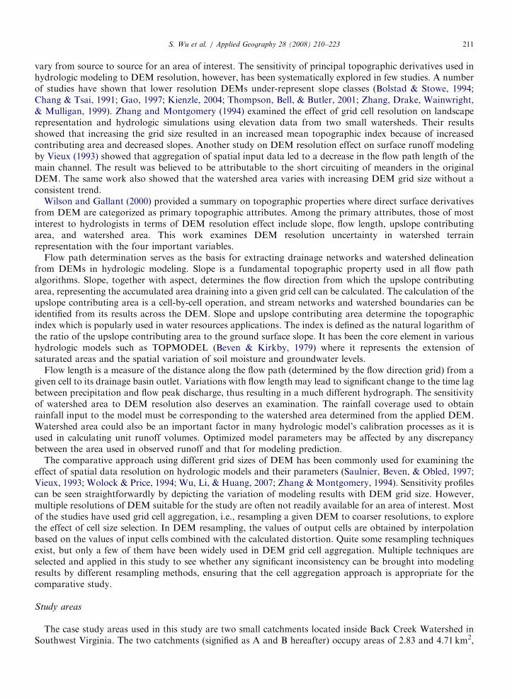
Fig. 2. Variations of mean slope and standard deviation with DEM grid size.


especially for Catchment B which has a higher gradient overall. The mean slope values for both catchmentsdrop significantly when the DEMs are resampled from the base resolution 10–30m (Fig. 2), while theobservation is much more pronounced for Catchment B. Apparently, the higher relief portion of each studyarea contributes a large part to the mean value decrease as presented in Fig. 3. The illustrations show that thedata aggregation can cause considerable reduction of steep slope angles, although the trends of the cumulativefrequency variations are the same for all the resolutions.

It can also be seen from Fig. 3 that the topography can be better preserved for a higher relief area duringgrid size aggregation. The slope values for Catchment B at the 200m resolution are still distributed with amaximum of about 251 (Fig. 3b) as compared to around 551 at 10m. On the other hand, the maximum slopevalue at 200m for Catchment A is less than 61, plunging from approximately 351 at 10m (Fig. 3a).

It is clear, based on Figs. 2 and 3, that choice of the resampling methods has no influence on the generalresult of DEM resolution effect on slope distribution at the watershed scale. Minor differences exist in theslope mean values and its distributions between the three applied resampling techniques for both study areas.It can be found that, the slope values in the bilinear interpolated DEMs are, on the whole, a little smaller thanthose obtained from the nearest neighbor resampling. On the contrary, the slopes in the DEMs from the cubicconvolution algorithm are generally greater than those of the nearest-neighbor method. The discrepancies canbe well explained by comparative characteristics of the resampling techniques. Bilinear interpolation computesthe output cell value using the weighted average of the nearest four input cells, and thus results in a smoothersurface than the nearest-neighbor method. Cubic convolution is similar to bilinear interpolation except thatthe weighted average is calculated from the 16 nearest input cell centers and their values. The fact thatsurrounding cells are involved brings about a problem to the calculation of output values for cells close to theDEM boundary. Both bilinear interpolation and cubic convolution may lead to unreasonable interpolated

ARTICLE IN PRESS

(a-1) Nearest neighbor

0.0

0.2

0.4

0.6

0.8

1.0

Cum

ulat

ive

frequ

ency

10m

30m

60m

100m

150m

200m

(a-2) Bilinear interpolation

0.0

0.2

0.4

0.6

0.8

1.0

Cum

ulat

ive

frequ

ency 10m

30m

60m

100m

150m

200m

(a-3) Cubic convolution

0.0

0.2

0.4

0.6

0.8

1.0

Cum

ulat

ive

frequ

ency

10m

30m

60m

100m

150m

200m

(b-1) Nearest Neighbor0.0

0.2

0.4

0.6

0.8

1.0

Cum

ulat

ive

frequ

ency 10m

30m

60m

100m

150m

200m

(b-2) Bilinear Interpolation0.0

0.2

0.4

0.6

0.8

1.0

Cum

ulat

ive

frequ

ency

10m

30m

60m

100m

150m

200m

(b-3) Cubic convolution0.0

0.2

0.4

0.6

0.8

1.0

0Slope (deg.)

Cum

ulat

ive

frequ

ency

10m

30m

60m

100m

150m

200m

50403020100Slope (deg.)

302520155 10

0Slope (deg.)

50403020100Slope (deg.)

302520155 10

0Slope (deg.)

50403020100Slope (deg.)

302520155 10

Fig. 3. Cumulative frequency distributions of slope: (a) Catchment A, (b) Catchment B.

S. Wu et al. / Applied Geography 28 (2008) 210–223 215

results around the DEM edge if background areas (no data) outside the given DEM are used for thoseclose-to-border cells. However, as 16 cells nearby are used in cubic convolution as compared to four cells inbilinear interpolation, the ‘‘edge effect’’ can be much more significant in an output DEM from cubicconvolution. The effect may produce more irregular surface close to the DEM boundary and cause higherslope values overall.

Upslope contributing area

A significant number of grid cells with zero flow accumulation on the DEMs of both catchments wereobserved when deriving distributions of the upslope contributing area with the D8 method applied. Theportions of cells with the zero value on the original 10m DEMs are 30.0% and 28.6%, respectively, forCatchment A and B. Grid cells with flow accumulation values of zero are local topographic highs, andgenerally correspond to peaks and ridgelines. The portion of zero value coverage increases generally for both

ARTICLE IN PRESS

Catchment A

0%

10%

20%

30%

40%

50%

60%

70%

DEM grid size (m)

Por

tion

of z

ero

cont

ribut

ing

area

Nearest neighbor


Cubic convolution

Catchment B

0%

10%

20%

30%

40%

50%

0DEM grid size (m)

Por

tion

of z

ero

cont

ribut

ing

area

Nearest neighbor


Cubic convolution

200150100500 20015010050

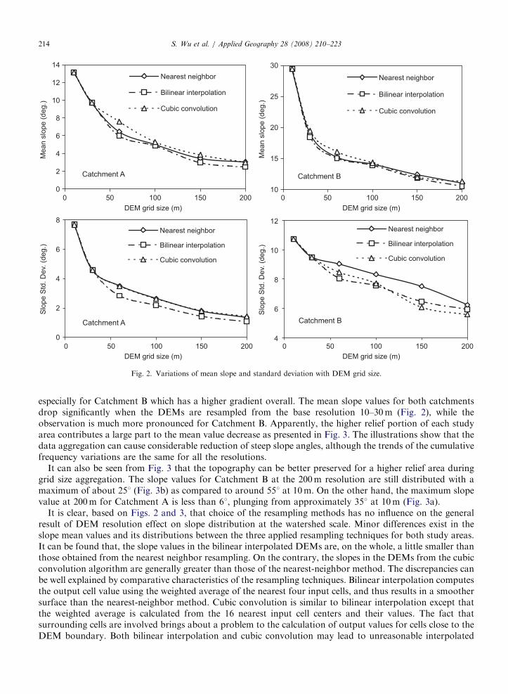
Fig. 4. Percentages of zero upslope contributing area at different DEM resolutions.


catchments with resampling to larger grid sizes, while fluctuation exists for most of the tests (Fig. 4). Aninteresting observation is that almost the same area value of zero flow accumulation for each catchment isobtained for different resampling methods when the DEM is first aggregated from 10 to 30m. Obviousdifferences in the percentage can, however, be seen among the resampled DEMs at 60m and higher grid sizes.It indicates that effect of resampling method comes up above a certain cell size (between 30 and 60m for eithercatchment). Over the threshold, areas of ridgelines and hilltops on three resampled DEMs at each cell size varyto a noticeable degree due to different interpolations with the resampling methods. Also apparently, theincrease of the zero flow accumulation area for Catchment A with the resampling is much more significantthan that for Catchment B. The portion of zero flow accumulation area for each of the three resampled DEMsat 200m is above 55% for Catchment A, while the percentages are all below 45% for Catchment B. This isbelieved to be attributable to the lower relief terrain in Catchment A.

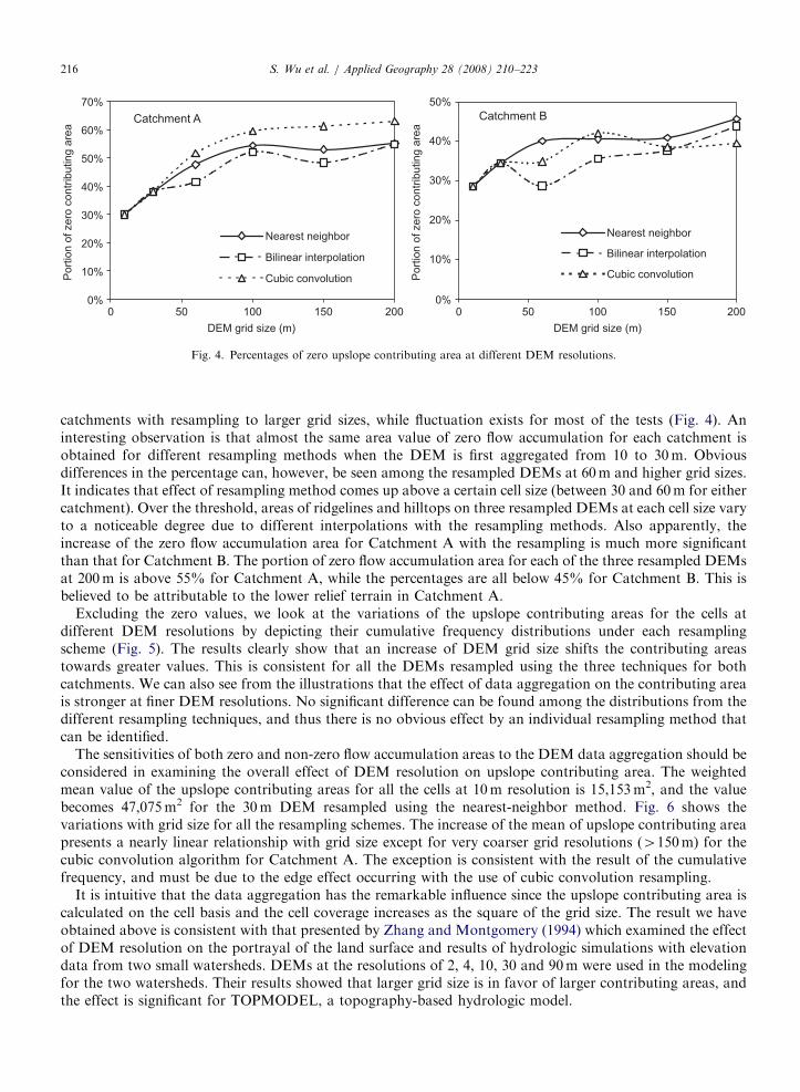
Excluding the zero values, we look at the variations of the upslope contributing areas for the cells atdifferent DEM resolutions by depicting their cumulative frequency distributions under each resamplingscheme (Fig. 5). The results clearly show that an increase of DEM grid size shifts the contributing areastowards greater values. This is consistent for all the DEMs resampled using the three techniques for bothcatchments. We can also see from the illustrations that the effect of data aggregation on the contributing areais stronger at finer DEM resolutions. No significant difference can be found among the distributions from thedifferent resampling techniques, and thus there is no obvious effect by an individual resampling method thatcan be identified.

The sensitivities of both zero and non-zero flow accumulation areas to the DEM data aggregation should beconsidered in examining the overall effect of DEM resolution on upslope contributing area. The weightedmean value of the upslope contributing areas for all the cells at 10m resolution is 15,153m2, and the valuebecomes 47,075m2 for the 30m DEM resampled using the nearest-neighbor method. Fig. 6 shows thevariations with grid size for all the resampling schemes. The increase of the mean of upslope contributing areapresents a nearly linear relationship with grid size except for very coarser grid resolutions (4150m) for thecubic convolution algorithm for Catchment A. The exception is consistent with the result of the cumulativefrequency, and must be due to the edge effect occurring with the use of cubic convolution resampling.

It is intuitive that the data aggregation has the remarkable influence since the upslope contributing area iscalculated on the cell basis and the cell coverage increases as the square of the grid size. The result we haveobtained above is consistent with that presented by Zhang and Montgomery (1994) which examined the effectof DEM resolution on the portrayal of the land surface and results of hydrologic simulations with elevationdata from two small watersheds. DEMs at the resolutions of 2, 4, 10, 30 and 90m were used in the modelingfor the two watersheds. Their results showed that larger grid size is in favor of larger contributing areas, andthe effect is significant for TOPMODEL, a topography-based hydrologic model.

ARTICLE IN PRESS

(a-1) Nearest Neighbor

0.4

0.5

0.6

0.7

0.8

0.9

1.0

Cum

ulat

ive

frequ

ency

10m30m60m100m150m200m

(a-2) Bilinear interpolation0.4

0.5

0.6

0.7

0.8

0.9

1.0

Cum

ulat

ive

frequ

ency

10m30m60m100m150m200m

(a-3) Cubic convolution0.5

0.6

0.7

0.8

0.9

1.0

Cum

ulat

ive

frequ

ency

10m

30m

60m

100m

150m

200m

(b-1) Nearest neighbor0.4

0.5

0.6

0.7

0.8

0.9

1.0

0Ln(a) [ln(m2)]

Cum

ulat

ive

frequ

ency

10m30m60m100m150m200m

(b-2) Bilinear interpolation0.4

0.5

0.6

0.7

0.8

0.9

1.0

Cum

ulat

ive

frequ

ency

10m30m60m100m150m200m


0.5

0.6

0.7

0.8

0.9

1.0

Cum

ulat

ive

frequ

ency

10m30m60m100m150m200m

1614121086420Ln(a) [ln(m2)]

161412108642

0Ln(a) [ln(m2)]

1614121086420Ln(a) [ln(m2)]

161412108642

0.40

Ln(a) [ln(m2)]1614121086420

Ln(a) [ln(m2)]161412108642

Fig. 5. Cumulative frequency distributions of upslope contributing area: (a) Catchment A, (b) Catchment B.


Flow length

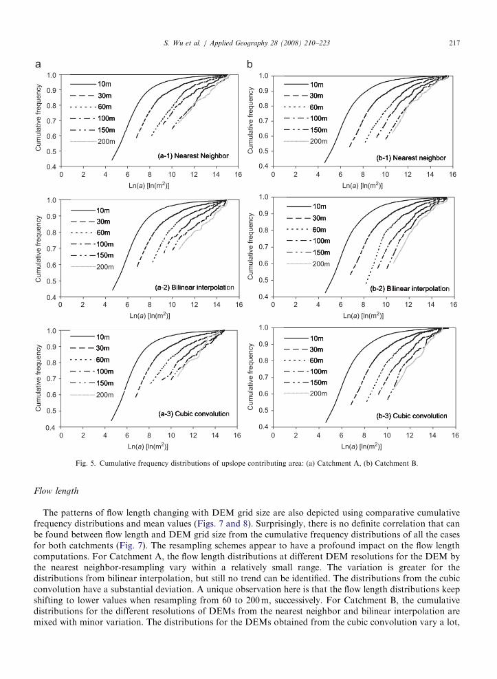
The patterns of flow length changing with DEM grid size are also depicted using comparative cumulativefrequency distributions and mean values (Figs. 7 and 8). Surprisingly, there is no definite correlation that canbe found between flow length and DEM grid size from the cumulative frequency distributions of all the casesfor both catchments (Fig. 7). The resampling schemes appear to have a profound impact on the flow lengthcomputations. For Catchment A, the flow length distributions at different DEM resolutions for the DEM bythe nearest neighbor-resampling vary within a relatively small range. The variation is greater for thedistributions from bilinear interpolation, but still no trend can be identified. The distributions from the cubicconvolution have a substantial deviation. A unique observation here is that the flow length distributions keepshifting to lower values when resampling from 60 to 200m, successively. For Catchment B, the cumulativedistributions for the different resolutions of DEMs from the nearest neighbor and bilinear interpolation aremixed with minor variation. The distributions for the DEMs obtained from the cubic convolution vary a lot,

ARTICLE IN PRESS

Catchment A0

50,000

100,000

150,000

200,000

250,000

300,000

DEM grid size (m)

Con

tribu

ting

area

per

cel

l (m

2 )C

ontri

butin

g ar

ea p

er c

ell (

m2 )

Nearest neighbor


Cubic convolution

Catchment B0

50,000

100,000

150,000

200,000

250,000

300,000

350,000

400,000

Nearest neighbor


Cubic convolution

0 20015010050

DEM grid size (m)0 20015010050

Fig. 6. Variations of mean upslope contributing area with DEM grid size.


but no correlation with grid size can be observed. These results are corroborated by the presentations in Fig. 8which shows variations of mean flow length values for all cells in the DEM with grid size. A commonobservation for all the three resampling cases for each catchment is that, when aggregating the DEM from 10to 30m, the flow length values shift a little higher with almost the same increase of the mean value. The curvesoscillate mostly for further increase of DEM grid size.

The length of the longest flow path is also calculated for each case, and the results are given in Fig. 9. Thevariation patterns for the longest flow length are nearly the same as those for mean flow length. These resultsdo not support the assertion from the published work by Vieux (1993) which investigated effects of dataaggregation on surface runoff modeling. The original 30m resolution DEM of a watershed was resampled tothree more DEMs of 90, 150, and 210m resolution, respectively, using the nearest-neighbor method. Thestudy found that meanders in the original DEM get short circuited as grid size increases with the aggregation,causing length reduction in flow paths.

Flow length is calculated based on the distance between center points of the cells along a flow path. Fromthe perspective of geometry, effect of DEM grid size on the length of a flow path depends mostly on the shapeof the flow path. DEM resampling to a greater cell size may lead to a reduction of flow length due to shortcircuit in a certain part of the entire flow path, but may also cause a longer route due to stretched distancesbetween enlarged cells in another section of the path. The overall impact of a grid size increase throughout the

ARTICLE IN PRESS

(a-3) Cubic convolution0.0

0.2

0.4

0.6

0.8

1.0

Cum

ulat

ive

frequ

ency 10m

30m60m100m150m200m

(a-1) Nearest neighbor0.0

0.2

0.4

0.6

0.8

1.0

0Flow length (m) Flow length (m)

Cum

ulat

ive

frequ

ency 10m

30m60m100m150m200m

(a-2) Bilinear interpolation

0.0

0.2

0.4

0.6

0.8

1.0

Cum

ulat

ive

frequ

ency 10m

30m60m100m150m200m

(b-1) Nearest neighbor0.0

0.2

0.4

0.6

0.8

1.0

Cum

ulat

ive

frequ

ency 10m

30m60m100m150m200m

(b-2) Bilinear interpolation0.0

0.2

0.4

0.6

0.8

1.0

Cum

ulat

ive

frequ

ency 10m

30m60m100m150m200m


0.2

0.4

0.6

0.8

1.0

Cum

ulat

ive

frequ

ency

10m30m60m100m150m200m

4,0003,0002,0001,000 0 4,0003,0002,0001,000


4,0003,0002,0001,000 0 4,0003,0002,0001,000


4,0003,0002,0001,000 0 4,0003,0002,0001,000

Fig. 7. Cumulative frequency distributions of flow length: (a) Catchment A, (b) Catchment B.


path determines the change of the flow path length. Therefore, increasing the grid size does not necessarilyresult in a shorter path as evidenced by the cases in this study.

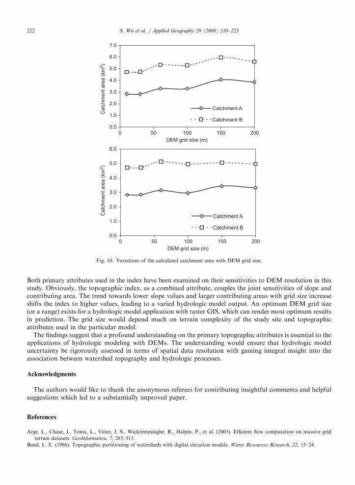
Watershed area

The DEM-based watershed area is determined with the cell size and number of cells in GIS. The variation ofcalculated areas for each catchment with DEM resampling in this study is shown in Fig. 10. The twocatchments possess a similar pattern of change with grid size. While the overall variation for both catchmentsappears to be a minor increase throughout the DEM resampling range, fluctuations are present within about+20% and +10% of the base areas (10m) for Catchments A and B, respectively. The variation of thecatchment area is due to the irregularity of resampled DEM boundaries, i.e., the boundaries are becoming

ARTICLE IN PRESS

Catchment A0

500

1,000

1,500

2,000

0DEM grid size (m)

Mea

n flo

w le

ngth

(m)

Nearest neighbor


Cubic convolution

Catchment B0

500

1,000

1,500

2,000

2,500

Mea

n flo

w le

ngth

(m)

Nearest neighbor


Cubic convolution

20015010050

0DEM grid size (m)

20015010050

Fig. 8. Variations of the mean flow length with DEM grid size.


more and more jagged with grid size increase. The effect is in a large part dependent on the shape of theoriginal map. The higher variation shown in Fig. 10 for Catchment A is attributable to its more irregularshape as well as its smaller area. A special case we may consider is an original DEM in a rectangle shape witheach side being a multiple of all grid sizes used for the comparative study. Any expected resampling will notcause any change to the DEM coverage in the circumstances.

Vieux (1993) also examined the effect of grid size change on the watershed area obtained from DEM, and noconsistent tendency is observed. The study believed that the area is varying because grid cells of different sizescannot consistently cover the irregular shape of the watershed. The perception is corroborated by the finding onwatershed area from this study. DEM aggregation may have influence on its calculated area, but the direction andextent of the effect would vary upon its base grid size, level of increase, and edge pattern of the DEM.

Summary and concluding remarks

Slope, upslope contributing area, flow path and watershed area are the four important topographic attri-butes determining watershed delineation and surface runoff profile in hydrologic modeling with raster-basedGIS. Effects of elevation data resolution on the four variables are analyzed across six different DEM grid sizesfor two watersheds with dissimilar overall gradient. Three commonly used resampling methods are utilized inorder to obtain more objective observations on the effects of DEM resolution.

ARTICLE IN PRESS

Catchment A0

1,000

2,000

3,000

4,000

Long

est f

low

leng

th (m

)

Nearest neighbor


Cubic convolution

Catchment B0

1,000

2,000

3,000

4,000

5,000

Long

est f

low

leng

th (m

)

Nearest neighbor


Cubic convolution

0DEM grid size (m)

20015010050

0DEM grid size (m)

20015010050

Fig. 9. Variations of the longest flow path length with DEM grid size.


Impacts are found for all the four examined derivatives as functions of DEM resolution. Slope estimates areseen constantly decreasing with the resolution growing coarser. The reduction is more profound for higherrelief areas at higher resolutions, indicating that the extent of smoothing effect would be varying with studyarea. Conversely, the estimates of upslope contributing area tend to increase along with the grid size increase.This is certainly true considering multiplied coverage area of each grid cell. The increase of mean contributingarea is roughly in linear relationship to grid size under fair DEM resolutions (o100m). No definite trend ofbias is observed for the calculations of flow path length and watershed area while both are sensitive to the gridsize change. It is suggested that the shape of each flow path plays a critical role in determining the response ofits flow length to grid resolution change. Similarly, the variation of DEM-based watershed area with grid sizedepends on the shape of map boundary. The higher the irregularity of the boundary shape, the moreunpredictable the effect on the watershed area estimate will be.

The above-examined effects on the primary attributes constitute the basis for DEM resolution uncertaintywith topographic and hydrologic characterization at watershed scale. The impacts will be conveyed tosecondary or compound topographic derivatives, which may be used as spatial input of a hydrologicmodel, thus resulting in uncertainty with prediction output. For example, TOPMODEL is a widely usedtopography-based model that simulates hydrologic fluxes of water through a watershed. The model isestablished on the assumption that the local hydraulic gradient is equal to the local surface slope, implyingthat all points with the same value of the topographic index will respond in a hydrologically similar way.

ARTICLE IN PRESS

0.0

1.0

2.0

3.0

4.0

5.0

6.0

7.0

Cat

chm

ent a

rea

(km

2 )C

atch

men

t are

a (k

m2 )

Catchment A

Catchment B

0.0

1.0

2.0

3.0

4.0

5.0

6.0

0DEM grid size (m)

Catchment A

Catchment B

20015010050

0DEM grid size (m)

20015010050

Fig. 10. Variations of the calculated catchment area with DEM grid size.


Both primary attributes used in the index have been examined on their sensitivities to DEM resolution in thisstudy. Obviously, the topographic index, as a combined attribute, couples the joint sensitivities of slope andcontributing area. The trend towards lower slope values and larger contributing areas with grid size increaseshifts the index to higher values, leading to a varied hydrologic model output. An optimum DEM grid size(or a range) exists for a hydrologic model application with raster GIS, which can render most optimum resultsin prediction. The grid size would depend much on terrain complexity of the study site and topographicattributes used in the particular model.

The findings suggest that a profound understanding on the primary topographic attributes is essential to theapplications of hydrologic modeling with DEMs. The understanding would ensure that hydrologic modeluncertainty be rigorously assessed in terms of spatial data resolution with gaining integral insight into theassociation between watershed topography and hydrologic processes.

Acknowledgments

The authors would like to thank the anonymous referees for contributing insightful comments and helpfulsuggestions which led to a substantially improved paper.

References

Arge, L., Chase, J., Toma, L., Vitter, J. S., Wickremesinghe, R., Halpin, P., et al. (2003). Efficient flow computation on massive grid

terrain datasets. GeoInformatica, 7, 283–313.

Band, L. E. (1986). Topographic partitioning of watersheds with digital elevation models. Water Resources Research, 22, 15–24.


Beven, K. J., & Kirkby, M. J. (1979). A physically based variable contributing area model of basin hydrology. Hydrological Science

Bulletin, 24, 43–69.

Bolstad, P., & Stowe, T. (1994). An evaluation of DEM accuracy: Elevation, slope, and aspect. Photogrammetric Engineering and Remote

Sensing, 60, 1327–1332.

Chang, K., & Tsai, B. (1991). The effect of DEM resolution on slope and aspect mapping. Cartography and Geographic Information

Systems, 18, 69–77.

Freeman, T. G. (1991). Calculating catchment area with divergent flow based on a regular grid. Computers and Geosciences, 17, 413–422.

Gao, J. (1997). Resolution and accuracy of terrain representations by grid DEMs at a micro-scale. International Journal of Geographical

Information Systems, 11, 199–212.

Garbrecht, J. & Martz, L.W. (1999). Digital elevation model issues in water resources modeling. In: Proceedings from invited water

resources sessions, 19th ESRI international user conference, (pp. 1–17).

Horn, B. K. P. (1981). Hill shading and the reflectance map. Proceedings of the IEEE, 69(1), 14–47.

Huang, G. H., & Chang, N. B. (2003). The perspectives of environmental informatics and systems analysis. Journal of Environmental

Informatics, 1, 1–7.

Jenson, S. K., & Domingue, J. O. (1988). Extracting topographic structure from digital elevation data for geographic information system

analysis. Photogrammetric Engineering and Remote Sensing, 54, 1593–1600.

Jones, K. H. (1998). A comparison of algorithms used to compute hill slope as a property of the DEM. Computers and Geosciences, 24,

315–323.

Keys, R. (1981). Cubic convolution interpolation for digital image processing. IEEE on Acoustics, Speech, and Signal Processing, 29,

1153–1160.

Kienzle, S. (2004). The effect of DEM raster resolution on first order, second order and compound terrain derivatives. Transactions in GIS,

8, 83–111.

Mitchell, D., & Netravali, A. (1988). Reconstruction filters in computer graphics. ACM Computer Graphics, 22, 221–228.

O’Callaghan, J. F., & Mark, D. M. (1984). The extraction of drainage networks from digital elevation data. Computer Vision, Graphics,

and Image Process, 28, 323–344.

Quinn, P., Beven, K. J., Chevallier, P., & Planchon, O. (1991). The prediction of hillslope flow paths for distributed hydrological modelling

using digital terrain models. Hydrological Processes, 5, 59–79.

Saulnier, G. M., Beven, K. J., & Obled, C. H. (1997). Digital elevation analysis for distributed hydrological modelling: reducing scale

dependence in effective hydraulic conductivity values. Water Resources Research, 33, 2097–2101.

Thompson, J. A., Bell, J. C., & Butler, C. A. (2001). Digital elevation model resolution: Effects on terrain attribute calculation and

quantitative soil-landscape modeling. Geoderma, 100, 67–89.

Vieux, B. E. (1993). DEM aggregation and smoothing effects on surface runoff modeling. Journal of Computing in Civil Engineering, 7,

310–338.

Wilson, J. P., & Gallant, J. C. (2000). Digital terrain analysis. In J. P. Wilson, & J. C. Gallant (Eds.), Terrain analysis (pp. 1–27).

New York: Wiley.

Wolock, D. M., & Price, C. V. (1994). Effects of digital elevation model map scale and data resolution on a topography-based watershed

model. Water Resources Research, 30, 3041–3052.

Wu, S., Li, J., & Huang, G. H. (2007). Modeling the effects of elevation data resolution on the performance of topography-based

watershed runoff simulation. Environmental Modelling & Software, 22, 1250–1260.

Zhang, X., Drake, N. A., Wainwright, J., & Mulligan, M. (1999). Comparison of slope estimates from low resolution DEMs: Scaling

issues and a fractal method for their solution. Earth Surface Processes and Landforms, 24, 763–779.

Zhang, W., & Montgomery, D. R. (1994). Digital elevation model grid size, landscape representation, and hydrologic simulations. Water

Resources Research, 30, 1019–1028.

a study on dem-derived primary topographic attributes for...

Documents