a study on out-of-vocabulary word modelling for a - citeseerx
TRANSCRIPT

A Study on Out-of-Vocabulary Word Modelling
for a
Segment-Based Keyword Spotting System
by
Alexandros Sterios Manos
B.S., Brown University, 1994
B.A., Brown University, 1994
Submitted to the Department of Electrical Engineering
and Computer Science
in partial ful�llment of the requirements for the degree of
Master of Science in Electrical Engineering and Computer Science
at the
MASSACHUSETTS INSTITUTE OF TECHNOLOGY
April 1996
c Massachusetts Institute of Technology 1996. All rights reserved.
Author : : : : : : : : : : : : : : : : : : : : : : : : : : : : : : : : : : : : : : : : : : : : : : : : : : : : : : : : : : : : :
Department of Electrical Engineering
and Computer Science
April, 1996
Certi�ed by : : : : : : : : : : : : : : : : : : : : : : : : : : : : : : : : : : : : : : : : : : : : : : : : : : : : : : : : :
Victor W. Zue
Senior Research Scientist
Thesis Supervisor
Accepted by : : : : : : : : : : : : : : : : : : : : : : : : : : : : : : : : : : : : : : : : : : : : : : : : : : : : : : : :
Frederic R. Morgenthaler
Chairman, Departmental Committee on Graduate Students

A Study on Out-of-Vocabulary Word Modeling for a Segment-Based
Keyword Spotting System
by
Alexandros S. Manos
Submitted to the Department of Electrical Engineering
and Computer Science
in May 9, 1996 in partial ful�llment of the
requirements for the degree of
Master of Science in Electrical Engineering and Computer Science
Abstract
The purpose of a word spotting system is to detect a certain set of keywords
in continuous speech. A number of applications for word spotting systems have
emerged over the past few years, such as automated operator services, pre-recorded
data indexing, and initiating human-machine interaction. Most word spotting systems
proposed so far are HMM based. The most common approach consists of models
of the keywords augmented with \�ller," or \garbage" models, that are trained to
account for non-keyword speech and background noise. Another approach is to use
a large vocabulary continuous speech recognition system (LVCSR) to produce the
most likely hypothesis string, and then search for the keywords in that string. The
latter approach yields much higher performance, but is signi�cantly more costly in
computation and the amount of training data required.
In this study, we develop a number of word spotting systems in an e�ort to
achieve performance comparable to the LVCSR, but with only a small fraction of
the vocabulary. We investigate a number of methods to model the keywords and
background, ranging from a few coarse general models (for the background only), to
re�ned phone representations, such as context-independent (CI), and word-dependent
(WD, only for keywords) models. The output hypothesis of the word spotter consists

of a sequence of phones and keywords, and there is no constraint on the number of
keywords per utterance.
The word spotters were developed using the segment-based SUMMIT speech
recognition system. The task is to detect sixty-one keywords from continuous speech
in the ATIS corpus. The training, development, and test sets are speci�cally de-
signed to contain the keywords in appropriate proportions. The keyword set consists
of thirty-nine cities, nine airlines, seven days of the week, and six other frequent words.
We have achieved performance of 89.8% Figure of Merit (FOM) for the LVCSR spot-
ter, 81.8% using CI phone-words as �ller models, and 79.2% using eighteen more
general models.
Thesis Supervisor: Victor W. Zue
Title: Senior Research Scientist
3

Acknowledgments
I would like to deeply thank my thesis supervisor, Victor Zue, for his guidance, sup-
port, and valuable advise. I thank Jim Glass for his support and patience, especially
during my �rst days in the world of speech recognition. I would also like to thank:
Mike McCandless for helping me understand the system and being available every
time I needed help; Michelle Spina for her encouragement and for being an out-
standing o�cemate and friend; Stephanie Sene� for her corrections and suggestions;
Christine Pao and Ed Hurley for keeping the system running; the rest of the peo-
ple in the Spoken Language Systems group, Jane, Giovanni, Sri, Ray and Ray, TJ,
Drew, Lee, Helen, DG, Joe, Vicky, Sally, Jim, Manish, Kenney and Grace for their
suggestions and the comfortable, friendly enviroment that they created.
Finally, I deeply thank my family for their love and for giving me the opportunity
to receive such an excellent education.
4

Contents
1 Introduction 101.1 De�nition of Problem : : : : : : : : : : : : : : : : : : : : : : : : : : : 101.2 Applications : : : : : : : : : : : : : : : : : : : : : : : : : : : : : : : : 101.3 Previous Research : : : : : : : : : : : : : : : : : : : : : : : : : : : : : 111.4 Discussion : : : : : : : : : : : : : : : : : : : : : : : : : : : : : : : : : 141.5 Outline : : : : : : : : : : : : : : : : : : : : : : : : : : : : : : : : : : : 14
2 Experimental Framework 162.1 Task : : : : : : : : : : : : : : : : : : : : : : : : : : : : : : : : : : : : 162.2 Corpus : : : : : : : : : : : : : : : : : : : : : : : : : : : : : : : : : : : 17
2.2.1 Data and Transcriptions : : : : : : : : : : : : : : : : : : : : : 182.2.2 Subsets : : : : : : : : : : : : : : : : : : : : : : : : : : : : : : 18
2.3 The SUMMIT Speech Recognition System : : : : : : : : : : : : : : : 202.3.1 Signal Representation : : : : : : : : : : : : : : : : : : : : : : : 212.3.2 Segmentation : : : : : : : : : : : : : : : : : : : : : : : : : : : 222.3.3 Measurements : : : : : : : : : : : : : : : : : : : : : : : : : : : 232.3.4 Acoustic Modeling : : : : : : : : : : : : : : : : : : : : : : : : 232.3.5 Pronunciation Network : : : : : : : : : : : : : : : : : : : : : : 232.3.6 Language Modeling : : : : : : : : : : : : : : : : : : : : : : : : 242.3.7 Search : : : : : : : : : : : : : : : : : : : : : : : : : : : : : : : 24
2.4 General Characteristics of Word Spotting Systems : : : : : : : : : : : 242.4.1 Training : : : : : : : : : : : : : : : : : : : : : : : : : : : : : : 25
2.5 Performance Measures : : : : : : : : : : : : : : : : : : : : : : : : : : 262.5.1 ROC curves and FOM : : : : : : : : : : : : : : : : : : : : : : 262.5.2 Computation Time : : : : : : : : : : : : : : : : : : : : : : : : 27
3 Large Vocabulary and Context-Independent Phone Word Spotters 283.1 Large Vocabulary Continuous-Speech Recognizer : : : : : : : : : : : : 28
3.1.1 Description of System : : : : : : : : : : : : : : : : : : : : : : 283.1.2 Results : : : : : : : : : : : : : : : : : : : : : : : : : : : : : : : 303.1.3 Error Analysis : : : : : : : : : : : : : : : : : : : : : : : : : : : 303.1.4 Conclusions : : : : : : : : : : : : : : : : : : : : : : : : : : : : 35
3.2 Context-Independent Phones as Fillers : : : : : : : : : : : : : : : : : 353.2.1 Description of System : : : : : : : : : : : : : : : : : : : : : : 363.2.2 Results : : : : : : : : : : : : : : : : : : : : : : : : : : : : : : : 37
5

3.2.3 Error Analysis : : : : : : : : : : : : : : : : : : : : : : : : : : : 383.2.4 Conclusions : : : : : : : : : : : : : : : : : : : : : : : : : : : : 42
3.3 Summary : : : : : : : : : : : : : : : : : : : : : : : : : : : : : : : : : 43
4 Word Spotters with General Filler Models 454.1 Clustering Methods : : : : : : : : : : : : : : : : : : : : : : : : : : : : 454.2 Word Spotter with 18 Filler Models : : : : : : : : : : : : : : : : : : : 50
4.2.1 Description of System : : : : : : : : : : : : : : : : : : : : : : 504.2.2 Results : : : : : : : : : : : : : : : : : : : : : : : : : : : : : : : 524.2.3 Error Analysis : : : : : : : : : : : : : : : : : : : : : : : : : : : 544.2.4 Conclusions : : : : : : : : : : : : : : : : : : : : : : : : : : : : 56
4.3 Word Spotter with 12 Filler Models : : : : : : : : : : : : : : : : : : : 574.3.1 Description of System : : : : : : : : : : : : : : : : : : : : : : 574.3.2 Results : : : : : : : : : : : : : : : : : : : : : : : : : : : : : : : 584.3.3 Error Analysis : : : : : : : : : : : : : : : : : : : : : : : : : : : 594.3.4 Conclusions : : : : : : : : : : : : : : : : : : : : : : : : : : : : 62
4.4 Word Spotter with 1 Filler Model : : : : : : : : : : : : : : : : : : : : 624.4.1 Description of System : : : : : : : : : : : : : : : : : : : : : : 624.4.2 Results : : : : : : : : : : : : : : : : : : : : : : : : : : : : : : : 634.4.3 Error Analysis : : : : : : : : : : : : : : : : : : : : : : : : : : : 634.4.4 Conclusions : : : : : : : : : : : : : : : : : : : : : : : : : : : : 66
4.5 Summary : : : : : : : : : : : : : : : : : : : : : : : : : : : : : : : : : 67
5 Word-Dependent Models for Keywords 685.1 Word-Dependent Models : : : : : : : : : : : : : : : : : : : : : : : : : 685.2 LVCSR Spotter with WD Models for the Keywords : : : : : : : : : : 70
5.2.1 Description of System and Results : : : : : : : : : : : : : : : 705.2.2 Comparison to LVCSR Spotter without WD Models : : : : : : 72
5.3 CI Spotter with WD Models for the Keywords : : : : : : : : : : : : : 755.3.1 Description of System and Results : : : : : : : : : : : : : : : 755.3.2 Comparison to CI Spotter without WD Models : : : : : : : : 76
5.4 Summary : : : : : : : : : : : : : : : : : : : : : : : : : : : : : : : : : 79
6 Summary and Improvements 816.1 Summary of Results : : : : : : : : : : : : : : : : : : : : : : : : : : : 81
6.1.1 FOM Performance : : : : : : : : : : : : : : : : : : : : : : : : 816.1.2 Computation Time : : : : : : : : : : : : : : : : : : : : : : : : 84
6.2 Improving Performance with Keyword-Speci�c Word-Boosts : : : : : 886.3 Future Work : : : : : : : : : : : : : : : : : : : : : : : : : : : : : : : : 90
6.3.1 Improvements and Flexibility : : : : : : : : : : : : : : : : : : 906.3.2 Possible Applications : : : : : : : : : : : : : : : : : : : : : : : 91
6

List of Figures
2-1 A block schematic of SUMMIT. : : : : : : : : : : : : : : : : : : : : : 202-2 MFSC �lter bank : : : : : : : : : : : : : : : : : : : : : : : : : : : : : 21
3-1 The Continuous Speech Recognition model. : : : : : : : : : : : : : : 293-2 Individual ROC curves for the LVCSR word spotter. : : : : : : : : : 313-3 Probability of detection as a function of the false alarm rate for the
LVCSR word spotter. : : : : : : : : : : : : : : : : : : : : : : : : : : : 333-4 Pronunciation network for the \word" sequence \f r { m boston t".
Only one arc per phone-word is allowed, while keywords are expandedto account for multiple pronunciations. : : : : : : : : : : : : : : : : : 36
3-5 Probability of detection as a function of the false alarm rate for theword spotter with context-independent phones as �llers. : : : : : : : : 38
3-6 Individual ROC curves for the word spotter with context-independentphones as �llers. : : : : : : : : : : : : : : : : : : : : : : : : : : : : : : 39
3-7 FOM and computation time measurements for the LVCSR and CIspotters. : : : : : : : : : : : : : : : : : : : : : : : : : : : : : : : : : : 44
4-1 Clustering of the 57 context-independent phones based on a confusionmatrix : : : : : : : : : : : : : : : : : : : : : : : : : : : : : : : : : : : 47
4-2 Clustering of the 57 context-independent phones based on the Eu-clidean distance between their vectors of means. : : : : : : : : : : : : 49
4-3 Probability of detection as a function of the false alarm rate for theword spotter with 18 general models as �llers. : : : : : : : : : : : : : 52
4-4 Individual ROC curves for the word spotter with 18 general models as�llers. : : : : : : : : : : : : : : : : : : : : : : : : : : : : : : : : : : : 53
4-5 Probability of detection as a function of the false alarm rate for theword spotter with 12 general models as �llers. : : : : : : : : : : : : : 58
4-6 Individual ROC curves for the word spotter with 12 general models as�llers. : : : : : : : : : : : : : : : : : : : : : : : : : : : : : : : : : : : 60
4-7 Probability of detection as a function of the false alarm rate for theword spotter with one �ller model. : : : : : : : : : : : : : : : : : : : 63
4-8 Individual ROC curves for the word spotter with one �ller model. : : 644-9 FOM and computation time measurements for the spotters with 18,
12, and 1 �ller models. The corresponding measurements for the CIspotter are shown for comparison. : : : : : : : : : : : : : : : : : : : : 67
7

5-1 Graph of FOM versus the smoothing parameter K, for the LVCSRspotter with word-dependent models. : : : : : : : : : : : : : : : : : : 71
5-2 Probability of detection as a function of the false alarm rate for theLVCSR spotter with word-dependent models for the keywords. : : : : 72
5-3 Individual ROC curves for the LVCSR spotter with word-dependentmodels for the keywords. : : : : : : : : : : : : : : : : : : : : : : : : : 73
5-4 Graph of FOM versus the smoothing parameterK, for the spotter withcontext-independent phones as �llers. : : : : : : : : : : : : : : : : : : 75
5-5 Probability of detection as a function of the false alarm rate for the CIspotter with word-dependent models for the keywords. : : : : : : : : 76
5-6 Individual ROC curves for the spotter with word-dependent models forthe keywords, and context-independent phones as �llers. : : : : : : : 77
5-7 FOM and computation time measurements for the LVCSR and CIspotters with and without word-dependent models. : : : : : : : : : : 80
6-1 FOM and computation time measurements for the all developed wordspotters. : : : : : : : : : : : : : : : : : : : : : : : : : : : : : : : : : : 87
8

List of Tables
2.1 The keywords chosen for word spotting in the ATIS domain : : : : : 172.2 Training, development and test sets. : : : : : : : : : : : : : : : : : : : 182.3 Keyword frequencies in each ATIS subset. : : : : : : : : : : : : : : : 19
3.1 Keyword substitutions for the LVCSR word spotter : : : : : : : : : : 323.2 Keyword substitutions for the word spotter with CI phones as �llers : 403.3 Most frequent transcription hypotheses for the word or sub-word \fare". 41
4.1 The context-independent phones composing the 18 clusters used asgeneral �ller models : : : : : : : : : : : : : : : : : : : : : : : : : : : : 51
4.2 Keyword substitutions for the word spotter with 18 general models as�llers : : : : : : : : : : : : : : : : : : : : : : : : : : : : : : : : : : : : 55
4.3 The context-independent phones composing the 12 clusters used asgeneral �ller models : : : : : : : : : : : : : : : : : : : : : : : : : : : : 57
4.4 Keyword substitutions for the word spotter with 12 general models as�llers : : : : : : : : : : : : : : : : : : : : : : : : : : : : : : : : : : : : 61
4.5 Keyword substitutions for the word spotter with 1 �ller model : : : : 65
5.1 Keyword substitutions for the LVCSR spotter with word-dependentmodels. : : : : : : : : : : : : : : : : : : : : : : : : : : : : : : : : : : 74
5.2 Keyword substitutions for the spotter with word-dependent models forthe keywords, and context-independent phones as �llers. : : : : : : : 78
6.1 FOM performance results for all developed word spotting systems. : : 826.2 Computation time results for all developed word spotting systems. : : 846.3 Performance improvements resulting from the introduction of keyword-
speci�c word-boosts. : : : : : : : : : : : : : : : : : : : : : : : : : : : 89
9

Chapter 1
Introduction
1.1 De�nition of Problem
Word spotting systems have the task of detecting a small vocabulary of keywords
from unconstrained speech. The word spotting problem is one of achieving the highest
possible keyword detection rate, while minimizing the number of keyword insertions.
Therefore, it is not su�cient to model only the keywords very explicitly, models of
the background are also required. In this study, we intend to show that representing
the non-keyword portions of the signal with increasingly more detailed models results
in improvement in keyword spotting performance.
1.2 Applications
In the past few years a lot of e�ort has been funneled into developing word spotting
systems for applications where the detection of just a few words is enough for a
transaction to take place. One such application that has already been introduced
to the market is automated operator services [13, 16], where the client is prompted
to speak the kind of service he/she wants, i.e., collect, calling-card, etc. Other such
services like Yellow Pages and directory assistance [1], can be implemented in similar
ways, only the vocabulary size will be signi�cantly larger.
10

Another application is audio indexing, where the task is to classify voice mail,
mixed-media recordings or even video by its audio context [7, 15]. The indexing is
performed based on su�cient occurrence of words particular to a domain of interest in
a section of the input signal. This application is extremely interesting, since it allows
scanning very large audio databases and extracting particular information without
having explicit knowledge of the entire vocabulary.
A third application is surveillance of telephone conversations for security reasons.
The spotting of certain words such as \buy" or \sell', or even \dollars" can point to
an information leak in the stock market telephone conversations.
Finally, word spotting can be used to initiate human-machine interaction. The
user can turn on his computer and his large vocabulary continuous-speech recogni-
tion system by saying a particular word. Furthermore, people with handicaps will be
able to control the opening of doors, switches, television sets, and many other house-
hold appliances by voice, using a word spotting system that only listens for speci�c
commands and disregards all other acoustic input.
1.3 Previous Research
Most of the word spotting systems proposed in the past years are HMM or neural
network based. The most common approach to word spotting systems design is to
create a network of keywords and complement it by \�ller," or \garbage" models,
that are trained to account for the non-keyword speech and background noise.
Rose [11] proposed an HMM word spotter based on a continuous-speech recogni-
tion model, and evaluated its performance on a task derived from the Switchboard
corpus [5]. In his study he evaluates the bene�ts to word spotting performance when
using (1) decision-tree based allophone clustering for de�ning acoustic sub-word mod-
els, (2) simple language models, and (3) di�erent representations for non-vocabulary
words. The word spotter uses a frame synchronous Viterbi beam search decoder,
where the keyword models compete in the �nite state network with the �ller mod-
els. The study concluded that reducing context-sensitive acoustic models to a small
11
number of equivalence classes, using allophone clustering, improved the performance
when models were under-trained. Including whole-words that appear in neighboring
positions to the keywords in the training set improved performance over general con-
text phonemes. Finally the use of a simple word-pair grammar improved results over
a null grammar network.
Jeanrenaud, et al. [6] propose a phonetic-based word spotter, and compare a
number of HMM con�gurations on the credit card phone conversations from the
Switchboard corpus. The number of keywords to be detected is twenty for this task.
The �rst con�guration uses a �ller model that contains �fty-six context-independent
phoneme models, trained from keyword and non-keyword data. The second system
uses a large vocabulary (2024 words) �ller model. The third system has the same
vocabulary, only it also incorporates a bigram language model. The fourth and �fth
systems use language modeling with reduced vocabulary (around 200) and a phoneme
loop. The performance for these systems ranged from 64% Figure of Merit (FOM,
de�nition in Section 2.5) for the con�guration with a simple phoneme �ller, to 79% for
the con�guration combining large vocabulary and language modeling. When the large
vocabulary system was used without a language model performance dropped to 71%.
From the above results it can be concluded that better modeling of the background
increases performance, language models give a boost even if the transcriptions on
which they are trained are only partial, and, �nally, choosing neighboring words for
modeling gives better results than choosing the most frequent ones in the training
set.
Lleida, et al. [8] conducted a number of experiments related to the problem of non-
keyword modeling and rejection in an HMM based Spanish word spotter. The task
was to detect the Spanish digits in unconstrained speech. The proposed system uses
a word-based HMM to model the keywords and three di�erent sets of �ller models to
represent the out-of-vocabulary words. The authors de�ne the sets of phonetic �llers,
syllabic �llers and word-based �llers. In the Spanish language more than 99% of the
allophonic sounds can be grouped into thirty-one phonetic units, which compose the
set of phonetic �llers. In order to constrain the number of syllables in the syllabic
12

set, the authors propose classifying the sounds into four broad classes; i.e., nasals and
liquids are one class, voiced obstruent consonants are another, etc. In that way, only
sixteen syllabic sets are needed to cover all the possible Spanish syllables. The third
�ller modeling set consists of a word-based �ller for monosyllabic words, another for
bi-syllabic words and a third one for words with more than three syllables. The results
of the above described experiments show that the best performance is achieved with
the syllabic �llers, followed by the phonetic �llers.
Weintraub [14] applies continuous-speech recognition (CSR) methods to the word
spotting task. A transcription is generated for the incoming speech by using a CSR
system, and any keywords that occur in the transcription are hypothesized. The
DECIPHER system uses a hierarchy of phonetic context-dependent models (CD)
such as biphones, triphones, word-dependent phones (WD), etc., as well as context-
independent (CI) phones to model words. The experiments described in the paper are
performed on the Air Travel Information System (ATIS) and the Credit Card tasks.
A bigram language model is incorporated, which treats all non-vocabulary words as
background. The �rst system described in the paper uses a �xed vocabulary with the
keywords and the N most common words (N between zero and full coverage), forcing
the recognition hypothesis to choose among the allowable words. The second system
adds a background model consisting of sixty context-independent models to the above
word list, thus allowing part of the input speech to be transcribed as background.
In the ATIS task, sixty-six keywords and their variants were chosen as keywords.
The �rst system, with a vocabulary of about 1200 words, achieved a FOM of 75.9%,
whereas the second system using a vocabulary consisting of only the keywords and
one background model with sixty CI phones achieved a FOM of 48.8%. The results
for the Credit Card task (twenty keywords), show that varying the vocabulary size
from medium to large does not have a great e�ect on the FOM performance, and the
system actually performs slightly better when the background model is left out of the
dictionary.
13

1.4 Discussion
The above papers were referenced in order to show that one of the most important
considerations in word spotting is the modeling of non-keyword speech. When a few,
general models are used as �llers, the recognizer often has the tendency to substitute
them for keywords, thus causing a large number of misses. On the other hand,
explicitly modeling every word in the background, as is done in large vocabulary
continuous-speech recognition systems (LVCSR), is computationally very expensive
and makes the recognizer structure rather complicated. The LVCSR approach to
word spotting, even though providing the best performance, also su�ers from the
fact that in many applications the full vocabulary of the domain is not known. If
the vocabulary coverage is not su�cient, the number of insertions is large, since the
system tries to account for unknown words by substituting them with the closest
known ones. In the following chapters, a set of experiments are proposed, which are
expected to demonstrate that when varying the complexity of the �llers from a few
very general models to explicit word models, there is a continuous improvement in
performance. The purpose of the thesis is to investigate a number of approaches to
background modeling, in an e�ort to �nd a middle ground between high recognizer
complexity and acceptable word spotting performance.
1.5 Outline
In the next chapter we provide a description of the ATIS domain, in which the word
spotting experiments are performed. The experimental framework is presented in
su�cient detail, and the measures of word spotting performance are de�ned and
analyzed. In Chapter 3, we begin the description of the systems developed for this
study with the LVCSR spotter, and the spotter with context-independent phones as
�llers. In Chapter 4, we start with a survey of various clustering methods for the
construction of more general �ller models. We then present the results for three word
spotters with eighteen, twelve, and one �ller models. Chapter 5 studies the e�ects
14

on word spotting performance when word-dependent models are introduced for the
keywords. Two systems with word-dependent models are developed, the LVCSR
spotter and the spotter with context-independent phones as �llers. In Chapter 6, a
systematic comparison of all the systems, with respect to performance as measured by
the FOM and computation time, is presented. A training procedure that improves the
FOM is proposed, and results are presented for some of the spotters. We conclude with
a discussion of future research directions and possible applications for the developed
word spotting systems.
15
Chapter 2
Experimental Framework
2.1 Task
All the experiments are performed in the ATIS [9, 2] domain. This domain has been
chosen because (1) the nature of the queries is such that recognizing certain keywords
may be su�cient to understand their meaning , (2) an LVCSR system has already been
developed for this domain, and (3) there is a lot of training and testing data available.
The task is the detection of sixty-one keywords in unconstrained speech. Furthermore,
the keyword has to be hypothesized in approximately the correct time interval of the
input utterance. The set of keywords was chosen out of the ATIS vocabulary as a
su�cient set for a hypothetical spoken language system. This system would enable
the client to enter information such as desired origin and destination point, fare basis,
and day of departure using speech. The breakdown of the keyword set is shown in
Table 2.1, and it consists of thirty-nine city names, nine airlines, the seven days of the
week, and six other frequently used words. The keywords were chosen to be of various
lengths in order to provide su�cient data for a comparison between word spotting
performance on short and on long words. For certain keywords (airfare, fare) we also
modeled their variants, i.e., \airfares" and \fares," but in measuring performance we
combined the putative hits, or insertions, of the keyword and its variants.
16

Cities Airlines Weekdays Freq. Words
atlanta baltimore american sunday airfareboston charlotte continental monday economychicago cincinnati delta tuesday farecleveland dallas eastern wednesday �rst classdallas fort worth denver northwest thursday round tripdetroit houston twa friday tomorrowindianapolis kansas city ua saturdaylas vegas los angeles usmemphis miami unitedmilwaukee minneapolismontreal nashvillenew york newarkoakland orlandophiladelphia phoenixpittsburgh saint louissaint petersburg salt lake citysan diego san franciscosan jose seattletampa torontowashington
Table 2.1: The keywords chosen for word spotting in the ATIS domain
2.2 Corpus
The corpora are con�gured from the ATIS [9, 2] task, which is the common evaluation
task for ARPA spoken language system developers. In the ATIS task, clients obtain
air travel information such as ight schedules, fares, and ground transportation from
a database using natural, spoken language. The initial ATIS task was based on a
database that only contained relevant information for eleven cities. Three corpora
(ATIS-0, 1, 2) were collected with this database through 1991. Consequently the
database was expanded to include air travel information for forty-six cities and �fty-
two airports in the US and Canada (ATIS-3).
17

2.2.1 Data and Transcriptions
Since 1990 nearly 25,000 ATIS utterances have been collected from about 730 speak-
ers. Only orthographic transcriptions are available for these utterances. The phonetic
transcriptions used for training and testing the word spotting systems presented in
this study were created by determining forced paths using the already existing LVCSR
system [18]. These transcriptions are not expected to be as accurate as those produced
by experienced professionals, but the size of the corpus makes manual transcription
prohibitive.
2.2.2 Subsets
The training, development, and test sets were derived from all the available data for
the ATIS task. The sets were speci�cally designed to contain all the keywords in
balanced proportions. The training set consists of approximately 10,000 utterances
selected from 584 speakers. Two development sets were created, \Dev1" and \Dev2",
the �rst consisting of 484 utterances from �fty-three speakers, and the second of 500
utterances from another �fty-three speakers. The test set consists of 1397 utterances
from thirty-six speakers, and contains over ten instances of each keyword. Table 2.2
describes the training, development, and test sets.
# keywords # utterances # speakers
Training set 15076 10000 584Dev1 set 765 484 53Dev2 set 807 500 53Test set 2222 1397 36
Table 2.2: Training, development and test sets.
The keywords, together with their frequency of occurrence in each of the training
and test sets, are shown in Table 2.3.
18

Keywords Training Dev1 Dev2 Test
airfare 81 9 7 38
american 326 16 9 48
atlanta 818 28 33 94
baltimore 555 18 14 36
boston 1318 40 44 139
charlotte 99 10 9 29
chicago 105 8 7 28
cincinnati 38 9 5 15
cleveland 88 10 10 27
continental 167 5 3 15
dallas 641 23 18 56
dallas fort worth 54 3 2 13
delta 332 15 19 76
denver 1033 36 36 57
detroit 65 5 7 16
eastern 62 1 6 19
economy 67 7 9 12
fare 1136 62 70 124
�rst class 375 13 14 51
friday 99 8 5 28
houston 58 4 1 25
indianapolis 103 6 6 25
kansas city 125 9 14 52
las vegas 97 11 4 32
los angeles 51 9 11 39
memphis 82 9 9 22
miami 104 11 11 26
milwaukee 143 15 21 37
minneapolis 85 7 4 21
monday 126 20 10 30
montreal 48 4 2 14
nashville 55 4 3 24
new york 146 11 5 37
newark 58 12 13 28
northwest 64 2 4 17
oakland 300 11 10 14
orlando 124 10 15 44
philadelphia 725 29 35 50
phoenix 95 9 9 33
pittsburgh 755 32 33 98
round trip 541 28 32 51
saint louis 73 5 7 14
saint petersburg 79 4 4 13
salt lake city 118 4 5 18
san diego 138 17 14 28
san francisco 1006 47 45 85
san jose 41 6 7 14
saturday 150 8 8 37
seattle 150 4 6 33
sunday 176 6 9 20
twa 51 4 2 14
tampa 28 6 2 21
thursday 177 11 11 19
tomorrow 84 9 3 14
toronto 149 17 17 38
tuesday 133 7 13 21
ua 53 2 1 15
us 243 18 22 75
united 203 8 11 17
washington 385 18 16 43
wednesday 286 14 25 35
Table 2.3: Keyword frequencies in each ATIS subset.
19

2.3 The SUMMIT Speech Recognition System
The word spotting systems developed for the set of experiments described in the
next section were based on the SUMMIT speech recognition system [17]. SUMMIT
is a segment-based, speaker-independent, continuous-speech recognition system, that
explicitly detects acoustic landmarks in the input signal, in order to extract acoustic-
phonetic features. There are three major components in the SUMMIT system. The
�rst component transforms the input speech signal into an acoustic-phonetic rep-
resentation. The second performs an expansion of baseform pronunciations into a
lexical network. The third component provides linguistic constraints in the search
through the lexical network. A schematic for SUMMIT is shown in Figure 2-1. In
what follows we give a brief but thorough description of all the components of the
SUMMIT system, and their function in training and testing.
Viterbi
Language Model
MFCCs
PCS
Dendrogram
Acoustic Phonetic Network
SpeechSignal
Classification A*
ProcessingSignal
Measurements
MatrixRotation 1-Best
N-best
Acoustic & DurationModels Pronunciation Net.
Segmentation
Figure 2-1: A block schematic of SUMMIT.
20

2.3.1 Signal Representation
The input signal is transformed into a Mel-Frequency Cepstral Coe�cient (MFCC)
representation through a number of steps. In the �rst processing step the signal
is normalized for amplitude, and the appropriate scaling is performed to bring the
maximum sample to 16 bits. Then the higher frequency components are enhanced
and the lower frequency components are attenuated by passing the signal through a
preemphasis �lter. The Short Time Fourier Transform (STFT) of the signal is then
computed, at an analysis rate of 200 Hz, using a 25.6 ms Hamming window. The
windowed signal is then transformed using a 512 point FFT, thus producing 1 frame
of spectral coe�cients every 5 ms.
In the next step the spectral coe�cients are processed by an auditory �lter
bank [12] to produce a Mel-Frequency Spectral Coe�cient (MFSC) representation.
The auditory �lter bank consists of forty triangular, constant-area �lters that are de-
signed to approximately model the frequency response of the human ear. The �lters
are arranged on a Mel-frequency scale that is linear up to 1000 Hz, and logarithmic
thereafter. They range in frequency between 156 and 6844 Hz as shown in Figure 2-2.
0 1000 2000 3000 4000 5000 6000 70000
0.2
0.4
0.6
0.8
1
Frequency (Hz)
Pow
er (
dB)
Figure 2-2: MFSC �lter bank
The logarithm of the signal energy in each �lter is computed, and the resulting
forty coe�cients compose the MFSC representation of the frame.
21

In the �nal processing step the MFSCs are transformed to a Mel-Frequency Cep-
stral Coe�cient (MFCC) representation through the cosine transformation shown in
Equation 2.1.
C[i] =NXj=1
S[j]cos[i(j �1
2)�
N] (2:1)
where
S[j] : MFSC coe�cient j
C[i] : MFCC coe�cient i
N : number of MFSC coe�cients
For our MFCC representation we use the �rst fourteen coe�cients. With this
representation each frame is characterized by a compact vector of fourteen numbers.
Another advantage of this cosine transformation is that the coe�cients are less cor-
related, and can be e�ectively modeled by independent densities. So after the signal
processing stage, the waveform is transformed into a sequence of 5 ms frames, and
each frame is characterized by fourteen MFCCs.
2.3.2 Segmentation
In the segmentation stage the new signal representation is used to establish explicit
acoustic landmarks that will enable subsequent feature extraction and phonetic label-
ing. In order to capture as many signi�cant acoustic events as possible, a multi-level
representation is used that delineates both gradual and abrupt changes in the signal.
The algorithm, as described in [3], associates a given frame with its neighbors, thus
producing acoustically homogeneous segments (i.e., segments in which the signal is
in some relative steady state). Acoustic boundaries are set whenever the association
direction of the frames switches from past to future. On the next higher level the
same procedure is repeated between regions instead of frames. The merging of regions
is continued until the entire utterance is represented by only one acoustic event. By
using the distance at which regions merge, a dendrogram can be composed, providing
a network of segment alternatives.
22

2.3.3 Measurements
Each one of the segments in the network developed above is described by a set of
thirty-six measurements. The set of measurements consists of a duration measure-
ment, and thirty-�ve MFCC averages within and across segment boundaries. The
measurements were determined by an automatic feature selection algorithm [10], that
was developed at MIT in an e�ort to combine human knowledge engineering with ma-
chine computational power. In the �rst training stage, the collection of measurement
vectors for all segments in the training set are rotated using principal component
analysis. The vectors are then scaled by the inverse covariance matrix of the entire
set of vectors. The rotation operation decorrelates the components of the vectors, and
the scaling operation adjusts their variance to one. The two operations are combined
into one matrix which is computed only once from all the training data. It is used
thereafter in the training and testing of all the developed word spotting systems.
2.3.4 Acoustic Modeling
Models for the acoustic units are calculated during training, and consist of mixtures
of any desired number of diagonal Gaussians in the 36-dimensional space de�ned by
the measurements. The duration of each acoustic unit is also separately modeled by
a mixture of Gaussians. In the experiments described in the following chapters, the
�fty-seven context-independent models are constrained to a maximum of twenty-�ve
mixtures of diagonal Gaussians. Although it has been proven that a larger number
of mixtures could provide better classi�cation performance, an upper bound had to
be imposed in order to keep computation time within reasonable limits.
2.3.5 Pronunciation Network
The words in the vocabulary are expanded into a pronunciation network based on a
set of phonological rules. Each word consists of a set of nodes and a set of labeled,
weighted arcs connecting the nodes. During training, the arc-weights acquire values
that re ect the likelihood of each allowed pronunciation. The nodes and arcs for each
23

word combined with the arcs corresponding to permissible word transitions form a
pronunciation network that is used in the search stage.
2.3.6 Language Modeling
The SUMMIT system can incorporate a unigram or bigram language model in the
search stage to produce the best-scoring hypothesis, and a trigram to produce N-best
hypotheses.
2.3.7 Search
During recognition, a vector of measurements is constructed for each proposed seg-
ment, and is compared to each of the phone models. Using the maximum a posteriori
probability decision rule, a vector of scores for the possible phone hypotheses is re-
turned for each segment. In the search stage, the Viterbi algorithm is used to �nd the
best path through the labeled segment network, using a pronunciation network and
a language model as constraints. In the case where more than one top scoring paths
are of interest, an A� search can be performed, providing the N-best hypotheses for
the input signal.
2.4 General Characteristics of Word Spotting Sys-
tems
The keyword spotting systems developed for this study are continuous-speech recog-
nition systems. They di�er from the conventional word spotters in that they propose
a transcription for the entire input utterance instead of just searching for the sec-
tion of the input signal that is most probable to be a keyword. They allow multiple
keywords to exist in one utterance, thus making applications such as audio indexing
feasible. Another important distinction of these systems from previously developed
word spotters is that they are segment-based instead of HMM or neural network
based. The use of such a recognizer is based on the belief that many of the acous-
24

tic cues for phonetic contrast are encoded at speci�c time intervals in the speech
signal. Establishing acoustic landmarks, as is done with segmentation, permits full
utilization of these acoustic attributes. A third distinction is in the training of the
language models. Conventionally, language models for word spotters were trained
on utterances with all background words represented by a single �ller model. This
grammar disregarded a lot of detail that could contain useful information. In the
proposed systems, the bigram language model is trained on the complete utterance
transcription, where each �ller model is treated as a distinct lexical entry.
2.4.1 Training
As mentioned in Section 2.2.1, there exist no phonetic transcriptions for the ATIS
corpus. In order to obtain such transcriptions, a forced search was performed using
the ATIS [18] recognizer and the existing utterance word orthographies.
In the �rst training stage all phone data are collected from the training utterances.
In order to decorrelate the measurements as much as possible, a principal component
analysis is performed on the combined data for all phones, producing a square 36-
dimensional rotation matrix. For all the consequent training and testing stages the
measurements of each segment are multiplied by this matrix. In the next training
stage the transcriptions created by the forced search are used to extract the data
relevant to each phone. These data are used in the computation of the acoustic
and duration models of the phones. Using these phone models and a pronunciation
network the forced paths are recomputed, and the new data are used to retrain the
acoustic and phonetic models. What follows is a series of corrective training steps,
where the weights on the pronunciation network arcs are set to equalize the number of
times an arc is missed and the number of times an arc is used incorrectly. Furthermore,
the weights of the phonetic models are also iteratively trained based on the matches
between lexical arcs and phonetic segments in the forced alignments. Training is
terminated when the hypothesized utterance matches the forced alignment as closely
as possible.
25

2.5 Performance Measures
2.5.1 ROC curves and FOM
The performance of the proposed word spotting systems is measured using conven-
tional Receiver Operating Characteristic (ROC) curves and FOM calculations. The
hypothesized keyword locations are �rst ordered by score for each keyword. The score
for the keywords is calculated as the sum of the segmentation, phonetic match, dura-
tion match, and language model scores for the segments that comprise it. A keyword
is considered successfully detected if the midpoint of the hypothesis falls within the
reference time interval. Then, a count of the number of words detected before the
occurence of the �rst, second, etc., false alarms is performed for each keyword. These
are the numbers of words that the recognizer would detect, if the threshold was set
at the score of each false alarm in turn. The detection rate for the word spotter is
calculated as the total number of keywords detected at that false alarm level, divided
by the total number of keywords in the test set.
Using the number of detections for each keyword separately, individual ROC
curves can be constructed. These curves allow comparisons in word spotting per-
formance among keywords, and enable comprehension of the word spotting system's
shortcomings.
A single FOM can be calculated as the average probability of detection up to ten
false alarms per keyword per hour, as shown in Equation 2.2.
FOM =1
10T
0@
NXj=1
p[j] + �p[N + 1]
1A
� = 10T �N (2.2)
where
T : Fraction of an hour of test talkers
N : First integer � 10T - 12
� : A factor that interpolates to 10 false alarms per hour
The FOM yields a mean performance for the word spotter in the range of acceptable
26
false alarm rates, and is a relatively stable statistic useful for comparison among word
spotting systems. In comparing the word spotters described in the following sections
we will mainly use the FOM measure, whereas keyword speci�c ROC curves and word
spotter ROC curves will only be used for error analysis.
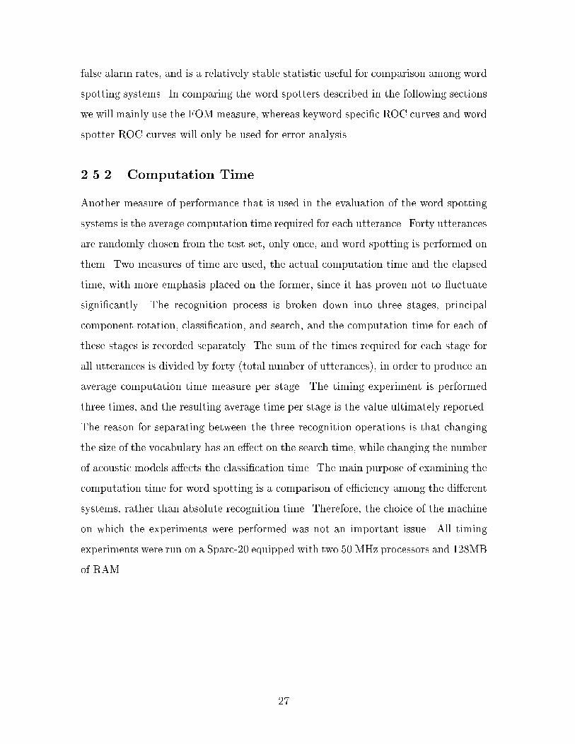
2.5.2 Computation Time
Another measure of performance that is used in the evaluation of the word spotting
systems is the average computation time required for each utterance. Forty utterances
are randomly chosen from the test set, only once, and word spotting is performed on
them. Two measures of time are used, the actual computation time and the elapsed
time, with more emphasis placed on the former, since it has proven not to uctuate
signi�cantly. The recognition process is broken down into three stages, principal
component rotation, classi�cation, and search, and the computation time for each of
these stages is recorded separately. The sum of the times required for each stage for
all utterances is divided by forty (total number of utterances), in order to produce an
average computation time measure per stage. The timing experiment is performed
three times, and the resulting average time per stage is the value ultimately reported.
The reason for separating between the three recognition operations is that changing
the size of the vocabulary has an e�ect on the search time, while changing the number
of acoustic models a�ects the classi�cation time. The main purpose of examining the
computation time for word spotting is a comparison of e�ciency among the di�erent
systems, rather than absolute recognition time. Therefore, the choice of the machine
on which the experiments were performed was not an important issue. All timing
experiments were run on a Sparc-20 equipped with two 50 MHz processors and 128MB
of RAM.
27

Chapter 3
Large Vocabulary and
Context-Independent Phone Word
Spotters
3.1 Large Vocabulary Continuous-Speech Recog-
nizer
3.1.1 Description of System
We begin the description of the word spotters developed for this thesis with the pre-
sentation of an LVCSR system. A schematic of the system is shown in Figure 3-1,
with �ller models being whole words. Any transition between words and keywords
is allowed, as well as self transitions for both words and keywords. A word spotting
system based on this model allows multiple keywords to exist in any one utterance, as
well as multiple instances of a keyword within the same utterance. The output of the
LVCSR is a complete word transcription of the input utterance. This recognizer uti-
28
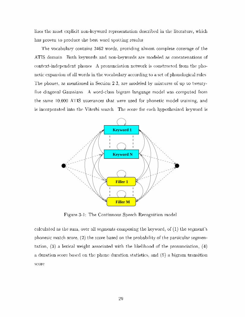
lizes the most explicit non-keyword representation described in the literature, which
has proven to produce the best word spotting results.
The vocabulary contains 2462 words, providing almost complete coverage of the
ATIS domain. Both keywords and non-keywords are modeled as concatenations of
context-independent phones. A pronunciation network is constructed from the pho-
netic expansion of all words in the vocabulary according to a set of phonological rules.
The phones, as mentioned in Section 2.3, are modeled by mixtures of up to twenty-
�ve diagonal Gaussians. A word-class bigram language model was computed from
the same 10,000 ATIS utterances that were used for phonetic model training, and
is incorporated into the Viterbi search. The score for each hypothesized keyword is
Keyword 1
Keyword N
Filler 1
Filler M
Figure 3-1: The Continuous Speech Recognition model.
calculated as the sum, over all segments composing the keyword, of (1) the segment's
phonetic match score, (2) the score based on the probability of the particular segmen-
tation, (3) a lexical weight associated with the likelihood of the pronunciation, (4)
a duration score based on the phone duration statistics, and (5) a bigram transition
score.
29

3.1.2 Results
The hypothesized transcription is parsed for the keywords, and a list of the scores
and time intervals of the hypothesized keywords is returned. For each test utterance
the list of hypothesized keywords is compared to the time aligned reference string,
and the occurrence of a detection or insertion is decided upon. The labeled data
(insertion or detection) for each keyword are collected and sorted with respect to
score from highest to lowest. Then the probability of detection (Pd) at each false
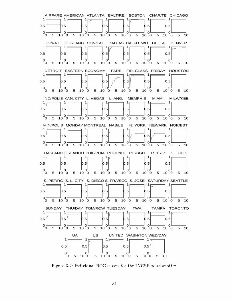
alarm rate is computed, and individual ROC curves are constructed for each keyword
(see Figure 3-2). In these plots Pd is normalized to one, and is reported as a function
of the number of false alarms per keyword per hour (fa/k/h). The reason for this time
normalization is that the number of false alarms that will be encountered at a given
performance level is proportional to the fraction of an hour that is spotted. The test
set used for the evaluation of the word spotting systems is a little over two hours,
making the pre-normalized number of false alarms misleadingly large. For the graphs
with no curve evident, the Pd is one before the �rst false alarm. The ROC curve for
the LVCSR as a word spotter for the sixty-one keywords is shown in Figure 3-3. The
�gure of merit for the word spotter was calculated to be 89.8%.
3.1.3 Error Analysis
The errors that occur during word spotting can be classi�ed as misses if the keyword
is not hypothesized in the correct location, and insertions if it is hypothesized in an
incorrect location. A miss and an insertion can be combined into a substitution, where
a keyword is inserted in the time location where another keyword should have been
hypothesized. Substitutions carry more weight than any of the other errors, because
they both decrease the probability of detection of the missed word and increase the
number of insertions of the falsely hypothesized keyword. In the LVCSR word spotting
system under examination the number of missed keywords was 154, with sixty-nine
of them being substitutions. The substitutions are shown in Table 3.1.
A number of interesting remarks can be made based on the data displayed in this
30
0 5 100
0.5
1AIRFARE
0 5 100
0.5
1AMERICAN
0 5 100
0.5
1ATLANTA
0 5 100
0.5
1BALT/RE
0 5 100
0.5
1BOSTON
0 5 100
0.5
1CHAR/TE
0 5 100
0.5
1CHICAGO
0 5 100
0.5
1CIN/ATI
0 5 100
0.5
1CLE/LAND
0 5 100
0.5
1CON/TAL
0 5 100
0.5
1DALLAS
0 5 100
0.5
1DA. FO. WO.
0 5 100
0.5
1DELTA
0 5 100
0.5
1DENVER
0 5 100
0.5
1DETROIT
0 5 100
0.5
1EASTERN
0 5 100
0.5
1ECONOMY
0 5 100
0.5
1FARE
0 5 100
0.5
1FIR. CLASS
0 5 100
0.5
1FRIDAY
0 5 100
0.5
1HOUSTON
0 5 100
0.5
1IND/POLIS
0 5 100
0.5
1KAN. CITY
0 5 100
0.5
1L. VEGAS
0 5 100
0.5
1L. ANG.
0 5 100
0.5
1MEMPHIS
0 5 100
0.5
1MIAMI
0 5 100
0.5
1MILW/KEE
0 5 100
0.5
1MIN/POLIS
0 5 100
0.5
1MONDAY
0 5 100
0.5
1MONTREAL
0 5 100
0.5
1NAS/LE
0 5 100
0.5
1N. YORK
0 5 100
0.5
1NEWARK
0 5 100
0.5
1NOR/EST
0 5 100
0.5
1OAKLAND
0 5 100
0.5
1ORLANDO
0 5 100
0.5
1PHIL/PHIA
0 5 100
0.5
1PHOENIX
0 5 100
0.5
1PIT/BGH
0 5 100
0.5
1R. TRIP
0 5 100
0.5
1S. LOUIS
0 5 100
0.5
1S. PET/RG
0 5 100
0.5
1S. L. CITY
0 5 100
0.5
1S. DIEGO
0 5 100
0.5
1S. FRA/SCO
0 5 100
0.5
1S. JOSE
0 5 100
0.5
1SATURDAY
0 5 100
0.5
1SEATTLE
0 5 100
0.5
1SUNDAY
0 5 100
0.5
1THU/DAY
0 5 100
0.5
1TOM/ROW
0 5 100
0.5
1TUESDAY
0 5 100
0.5
1TWA
0 5 100
0.5
1TAMPA
0 5 100
0.5
1TORONTO
0 5 100
0.5
1UA
0 5 100
0.5
1US
0 5 100
0.5
1UNITED
0 5 100
0.5
1WASH/TON
0 5 100
0.5
1WED/DAY
Figure 3-2: Individual ROC curves for the LVCSR word spotter.
31

Actual Hypothesized Frequency
airfare fare 13
newark new york 9
new york newark 6
tampa atlanta 3
orlando atlanta 3
las vegas boston 2
tampa denver 2
orlando denver 2
sunday saturday 2
fare san francisco 2
atlanta toronto 1
boston baltimore 1
boston nashville 1
chicago atlanta 1
dallas fort worth dallas 1
economy denver 1
economy houston 1
fare philadelphia 1
friday sunday 1
indianapolis minneapolis 1
miami montreal 1
minneapolis indianapolis 1
monday sunday 1
saint petersburg pittsburgh 1
san diego los angeles 1
san jose saturday 1
san jose wednesday 1
saturday newark 1
seattle fare 1
sunday san diego 1
thursday wednesday 1
tomorrow atlanta 1
tomorrow houston 1
toronto denver 1
us ua 1
Table 3.1: Keyword substitutions for the LVCSR word spotter
32

0 1 2 3 4 5 6 7 8 9 100
0.1
0.2
0.3
0.4
0.5
0.6
0.7
0.8
0.9
1
False Alarms/Keyword/Hour
Pd
Figure 3-3: Probability of detection as a function of the false alarm rate for theLVCSR word spotter.
table. The keywords \fare" and \airfare" are the most confused pair, with one of the
keywords being a sub-word of the other. Since in the ATIS domain the words \fare"
and \airfare" carry the same information their recognition results can be combined,
thus improving both their individual performance and that of the word spotter. This
might not be the case in another domain though, where the type of fare is an important
factor in the correct understanding of the query. The next most confused keywords
are \newark" and \new york", which is not surprising at all since they are acoustically
very similar. The only signi�cant distinctions in the pronunciation of the two words
are in the semi-vowels /w/ and /y/, which are highly confused sounds, and in their
stress pattern. The confusion between \atlanta" and \tampa" is a little bit more
subtle, but can be explained when noticing that both words end with the phone
sequence [/@/ nasal stop /{/]. Stops are highly confused as well as nasals within
their own classes, thus allowing such recognition errors. In general, substitutions
occurred most frequently between keywords that are acoustically similar and belong
in the same word-class, since in that case the language model component cannot
prevent the error. Across word-class substitutions accounted for only 16.7% of the
total substitutions.
33

From Figure 3-2, the keywords that demonstrated poor word spotting performance
can easily be identi�ed. For the keyword \airfare" almost all of the errors are of the
substitution type, as explained above. On the other hand, the word \economy"
was only substituted once by \denver," while the other three misses were due to
non-keyword word strings being hypothesized in its place. It is important to note
that \economy" occurred only twelve times in the test set, and furthermore was
one of the least frequent words in all sets, suggesting a high probability of poor
training. One of the keywords that performed very poorly, according to its ROC
graph, was the word \fare". The number of times it was missed though was only
seven out of 124 occurrences, indicating that insertions rather than misses were the
main factor degrading this keyword's performance. Indeed, closer examination of
the sorted and labeled data shows that the �rst eight pre-normalized insertions (or
approximately four when normalized for time) are due to \airfare" being inserted.
If the two keywords were grouped, the Pd at 1 fa/k/h would be approximately 0.5.
Another interesting recognition error that occurred was identi�ed by investigation
of the very low performance of the keyword \tomorrow". This word was missed
exactly half of the time (seven out of fourteen) due to insertions being allowed in
the Viterbi path, and the existence of the inter-word trash (iwt) model which is
added in the pronunciation network at the end of all words to account for possible
dis uencies in spontaneous speech. In searching for the path with the highest score
in the segmentation network, the cumulative score of the segments composing a word
is sometimes lower than the score of a large segment labeled as inter-word trash or
insertion. This e�ect, combined with a very low bigram transition score, caused the
keyword \tomorrow" to be completely overwritten by the word \ ight" that preceded
it in six of the seven utterances.
In conclusion, the main source of errors for the LVCSR word spotter was the
substitution between acoustically similar keywords, and only to a small degree the
incorporation in the search of insertions and the inter-word trash model. In an exper-
iment where insertions and iwt models where removed, some of the misses of \tomor-
row" were converted to detections, but the overall performance of the word spotter
34

dropped, indicating that their collective bene�t outweighs the low performance on
one of the words spotted.
3.1.4 Conclusions
The large vocabulary continuous speech recognition word spotting system described
in this section will be the bench mark against which all other word spotting systems
will be evaluated. The background modeling for this recognizer is the most explicit
presented in this thesis, and the achieved performance as measured by the FOM the
highest (89.8%), when only context independent phones are used in word modeling.
The ROC curve for the word spotter rises rapidly, crossing the 90% probability of
detection margin before 4 fa/k/h, and rising up to 92.7% at 10 fa/k/h. The tradeo�
for this outstanding word spotting performance is the rather long computation time1
required due to the size of the vocabulary. Although the LVCSR word spotter provides
the best spotting accuracy, it also requires more computation time and memory than
any of the word spotting systems developed in the following sections.
3.2 Context-Independent Phones as Fillers
In the previous section we described an LVCSR word spotting system that uses the
most explicit �ller models, i.e., whole words, and achieves outstanding accuracy as
measured by the FOM. One of the most important disadvantages of using a large
vocabulary recognizer for spotting purposes is the large amount of computation re-
quired, which is due to the large size of the vocabulary used. In an e�ort to design
a system that achieves performance approaching that of the LVCSR spotter, but
with signi�cant savings in computation time, we designed a series of systems that
use increasingly fewer, more general �ller models. The �rst of these systems, with
context-independent phones composing the background, is presented in this section.
1The timing results will be shown as a comparison in Section 6.1.2, after all word spotters havebeen introduced.
35

3.2.1 Description of System
This word spotter is again a continuous speech recognition system based on the
schematic of Figure 3-1. The vocabulary consists of the sixty-one keywords and
their variants, with the addition of �fty-seven phone-words corresponding to context-
independent phones. Any transition from keyword to phone-word and vice-versa is
allowed, as well as transitions within the two sets. This continuous speech recogni-
tion system will hopefully produce sequences of phones for the non-keyword sections
of the input signal, and whole words for the sections where the probability of key-
word existence is high. The phone-words consist of a single arc in the pronunciation
network, while all keywords are phonetically expanded as shown in Figure 3-4. The
ax mf r
bcl b
boston
s tcl t ax nb ao
en nx
t
Figure 3-4: Pronunciation network for the \word" sequence \f r { m boston t".Only one arc per phone-word is allowed, while keywords are expanded to account formultiple pronunciations.
only di�erence in the pronunciations allowed for the keywords in this word spotting
system compared to those for the LVCSR spotter is that the inter-word trash (iwt)
arcs have been removed. The justi�cation for this modi�cation lies in the fact that
the iwt phone-word has been added to the lexicon in order to model dis uencies in
spontaneous speech.
In order to train a language model for this word spotter we had to manipulate
the training utterances in such a way as to resemble the actual output of the spotter.
Using the LVCSR system and the available orthographic transcriptions we performed
a forced search that produced transcriptions consisting of phones for the non-keyword
words, and whole words for the keywords. These new transcriptions where used to
36

train a bigram language model for the keywords and the phone-words. They were also
used as reference orthographies for the computation of forced paths in the training
of the acoustic models and the lexicon arc weights.
The score for each hypothesized keyword is composed of the same sub-scores as for
the LVCSR system. There are three factors that control the decision of hypothesizing
a keyword versus hypothesizing the underlying string of phones. The �rst one is
the combined e�ect of the word transition weight (wtw) and the segment transition
weight (stw), which are trainable parameters. The wtw corresponds to a penalty for
the transition into a new word, while the stw is a bonus for entering a new segment.
During training, these parameters acquire appropriate values, in order to equalize
the number of words in the reference string and the hypothesized string. The second
factor is the bigram transition score, which consists only of the transition score into the
keyword in the �rst case, versus the sum of the bigram transition scores between each
of the underlying phone-words in the second case. The language model component
was trained from utterances where keywords were represented as whole words, in an
e�ort to prevent the composition of large bigram scores for the underlying phone-
words. Finally, the arcs representing transitions between phones within the keywords
carry weights that are added to the keyword score. Since these arc-weights can be
either positive or negative, depending on the likelihood of the pronunciation path to
which they belong, they can in uence the keyword hypothesis either way.
3.2.2 Results
The scores for all the hypothesized keywords are collected and labeled according to
the procedure described in the previous section. The ROC curve for the word spotter
with context-independent phones as �llers is shown in Figure 3-5. It is immediately
obvious that the area over the curve has increased compared to the LVCSR spotter
indicating a drop in performance. The ROC curves for each individual keyword are
shown in Figure 3-6. The FOM was calculated to be 81.8%, approximately 8% lower
in absolute value than that of the LVCSR system.
37

0 1 2 3 4 5 6 7 8 9 100
0.1
0.2
0.3
0.4
0.5
0.6
0.7
0.8
0.9
1
False Alarms/Keyword/Hour
Pd
Figure 3-5: Probability of detection as a function of the false alarm rate for the wordspotter with context-independent phones as �llers.
3.2.3 Error Analysis
We start the error analysis for this system by analyzing the substitution errors that
occurred during spotting. The total number of missed keywords was 321, out of
which only sixty-seven were substitutions. The number of missed keywords more
than doubled compared to the LVCSR spotter, while the number of substitutions
remained relatively stable. The substitution pairs are shown in Table 3.2. There are
many similarities between this table and Table 3.1. The top three most frequently
confused keywords are the same, but their frequency of substitution has dropped
signi�cantly. Again \new york" and \newark" were very frequently confused due
to their acoustic similarity, as well as \tampa" and \atlanta," \minneapolis" and
\indianapolis." Six of the substitutions of \airfare" by \fare" in the LVCSR spotter
have become misses in this recognizer. The percentage of substituted keyword pairs
that did not belong in the same word-class for this word spotter was 37.3%, indicating
that the language model constraint was not as e�ective here as it was in the LVCSR
spotter. Overall, this system demonstrated substitutions mostly between acoustically
confused keywords. The number of across word-class substitution pairs increased
38

0 5 100
0.5
1AIRFARE
0 5 100
0.5
1AMERICAN
0 5 100
0.5
1ATLANTA
0 5 100
0.5
1BALT/RE
0 5 100
0.5
1BOSTON
0 5 100
0.5
1CHAR/TE
0 5 100
0.5
1CHICAGO
0 5 100
0.5
1CIN/ATI
0 5 100
0.5
1CLE/LAND
0 5 100
0.5
1CON/TAL
0 5 100
0.5
1DALLAS
0 5 100
0.5
1DA. FO. WO.
0 5 100
0.5
1DELTA
0 5 100
0.5
1DENVER
0 5 100
0.5
1DETROIT
0 5 100
0.5
1EASTERN
0 5 100
0.5
1ECONOMY
0 5 100
0.5
1FARE
0 5 100
0.5
1FIR. CLASS
0 5 100
0.5
1FRIDAY
0 5 100
0.5
1HOUSTON
0 5 100
0.5
1IND/POLIS
0 5 100
0.5
1KAN. CITY
0 5 100
0.5
1L. VEGAS
0 5 100
0.5
1L. ANG.
0 5 100
0.5
1MEMPHIS
0 5 100
0.5
1MIAMI
0 5 100
0.5
1MILW/KEE
0 5 100
0.5
1MIN/POLIS
0 5 100
0.5
1MONDAY
0 5 100
0.5
1MONTREAL
0 5 100
0.5
1NAS/LE
0 5 100
0.5
1N. YORK
0 5 100
0.5
1NEWARK
0 5 100
0.5
1NOR/EST
0 5 100
0.5
1OAKLAND
0 5 100
0.5
1ORLANDO
0 5 100
0.5
1PHIL/PHIA
0 5 100
0.5
1PHOENIX
0 5 100
0.5
1PIT/BGH
0 5 100
0.5
1R. TRIP
0 5 100
0.5
1S. LOUIS
0 5 100
0.5
1S. PET/RG
0 5 100
0.5
1S. L. CITY
0 5 100
0.5
1S. DIEGO
0 5 100
0.5
1S. FRA/SCO
0 5 100
0.5
1S. JOSE
0 5 100
0.5
1SATURDAY
0 5 100
0.5
1SEATTLE
0 5 100
0.5
1SUNDAY
0 5 100
0.5
1THU/DAY
0 5 100
0.5
1TOM/ROW
0 5 100
0.5
1TUESDAY
0 5 100
0.5
1TWA
0 5 100
0.5
1TAMPA
0 5 100
0.5
1TORONTO
0 5 100
0.5
1UA
0 5 100
0.5
1US
0 5 100
0.5
1UNITED
0 5 100
0.5
1WASH/TON
0 5 100
0.5
1WED/DAY
Figure 3-6: Individual ROC curves for the word spotter with context-independentphones as �llers.
39

Actual Hypothesized Frequency
newark new york 8
airfare fare 7
new york newark 3
tampa atlanta 3
minneapolis indianapolis 3
us fare 2
american newark 1
chicago cleveland 1
chicago economy 1
cincinatti san francisco 1
continental atlanta 1
dallas dallas fort worth 1
dallas fort worth dallas 1
denver fare 1
fare san francisco 1
fare thursday 1
fare wednesday 1
�rst class fare 1
�rst class san francisco 1
indianapolis minneapolis 1
los angeles thursday 1
montreal baltimore 1
nashville atlanta 1
nashville boston 1
nashville fare 1
nashville tomorrow 1
newark american 1
northwest delta 1
northwest denver 1
northwest thursday 1
oakland fare 1
orlando atlanta 1
orlando denver 1
pittsburgh tuesday 1
round trip fare 1
saint petersburg pittsburgh 1
san jose wednesday 1
seattle toronto 1
tampa cleveland 1
tampa fare 1
thursday wednesday 1
ua tuesday 1
us saint louis 1
us ua 1
us wednesday 1
washington seattle 1
wednesday sunday 1
Table 3.2: Keyword substitutions for the word spotter with CI phones as �llers
40

signi�cantly with respect to the LVCSR.
One of the most frequently occurring errors is connected to the poor performance
of the keywords \fare" and \airfare." Table 3.3 lists the most frequent transcriptions
that the spotter hypothesized in place of the actual keyword for the missed instances.
Starting with the most frequent error, while the sequence [/f/ /∑/ /E / /r/] is a valid
Transcription Frequency
f ∑E r 7f ∑E r { m 4T 5v z 3T 5s 3f ∑E r | z 2f ∑E r { n 2
Table 3.3: Most frequent transcription hypotheses for the word or sub-word \fare".
pronunciation for the keyword \fare," it receives a higher score as a sequence of phone
words than as a keyword. In analyzing the individual score components we discov-
ered that (1) the arc-weights for the particular pronunciation are all positive, thus
supporting the keyword hypothesis, (2) the sum of the bigram transitions between
the phone-words is less than the bigram transition into the keyword, thus favoring
the former, and (3) the sum of four wtw's for the sequence, a large negative number,
is less than the sum of one wtw and three stw's, a positive number, for the keyword.
Therefore, it seems that the language model score is the key factor that controls when
the keyword is hypothesized over the string of phone-words. This conclusion is fur-
ther veri�ed by the fact that in all cases that the keyword was correctly hypothesized,
when pronounced in the manner under discussion, it received a larger bigram score
than the sum of the bigram scores of the underlying phones. This phenomenon is due
to the use of the bigram language model which can only collect very local informa-
tion for each word. In this system, the decomposition of the non-keyword words into
strings of phones created an asymmetry in the amount of data available for keyword
versus phone-word training. Any pair of phone-words potentially received counts for
the language model from instances belonging to many di�erent words. In particular,
41

frequent words such as \for" and \from" gave rise to sequences of phone-words sim-
ilar to the pronunciation of the keyword \fare." The type of error under discussion
occurs mostly in short words where the arc-weights and the stw's do not get a chance
to add enough support to the keyword hypothesis. The rest of the rows in Table 3.3
list other frequent substitutions of \fare" by well-trained strings of phone-words, such
as \/r/ /{/ /m/" in the second row, which is trained from the decomposition of the
very frequent ATIS word \from." In the third and fourth rows, the labial fricative
/f/ is confused with the dental fricative /T /, and the total bigram score favors again
the string of phone words instead of the keyword variant \fares."
A similar error is the cause for the keyword \nashville" being missed more than
half of the time. The hypothesized transcription for these missed instances is almost
in all cases [/n/ /e/ /S / /o/]. The fact that /o/ is consistently hypothesized after /S /
can be due to two factors, (1) the language model is trained on the phone sequence
corresponding to the very frequent word \show," thus the bigram transition from /S /
to /o/ carries a very large weight, and (2) the front vowels /I/ or /| / become similar
to /o/ when in the context of the labial fricative /v/ on the left forcing all formants
down, and the semi-vowel /l/ on the right, forcing the second formant down. A few
other words such as \tomorrow," \tampa," and \ua" demonstrated poor spotting
performance for reasons similar to those already discussed. In general, most errors
can be explained by substitutions due to acoustic similarity between keywords, and
the e�ects of the bigram language model which frequently favors sequences of phone-
words over keywords.
3.2.4 Conclusions
This section described the �rst e�ort to develop a system that achieves performance
approaching that of the large vocabulary keyword spotter, while using a much shorter
and compact background representation. The FOM for this spotter is about 8% lower
in absolute value than that of the LVCSR system, but it is still very high. Comparison
of the ROC curves for the two systems leads to the observation that the probability
of detection as a function of the fa/k/h rises faster for the phone-word system. An
42

important consequence is that, at 5 fa/k/h, this spotter's Pd only di�ers by approxi-
mately 6.5% from that of the LVCSR spotter. The main source of error for the system
under discussion was the substitution of keywords by strings of phone-words that car-
ried a very large cumulative bigram transition score. An improved language model
that would compensate for some of the high probability for the bigram transitions
between phone-words, and therefore favor the hypothesis of keywords, could result in
signi�cant improvement in performance. Another way of achieving the same result
would be to add a word-speci�c boost to each keyword, in order to favor it being
hypothesized over the phone-words. The appropriate values for these word-boosts
can be decided upon through an iterative optimization process that tries to equalize
the number of insertions and deletions of the keywords, or maximize the overall FOM.
The possibility of improvement is also supported by the fact that for the majority of
keywords the number of insertions is very low, and all the detections occur before even
the �rst insertion. In other words, due to the very low number of insertions, there
is a good chance that favoring the keywords with word-speci�c boosts could improve
the overall performance by trading misses with insertions. Some experimental results
showing signi�cant improvement in performance when incorporating word-boosts are
discussed in Section 6.2.
The computation time for this system was calculated under the same conditions
as the LVCSR system. As expected, the Viterbi stage of the recognition process was
approximately seven times as fast2 as that of the LVCSR. In conclusion, the system
presented in this section managed to signi�cantly reduce the computation time, while
still providing very good word spotting performance as measured by the FOM.
3.3 Summary
In this chapter we described two word spotting systems with very di�erent background
representations. The �rst system (LVCSR) used explicit models of all words in the
2The timing results will be discussed in detail in Section 6.1.2, after all word spotters have beenintroduced.
43

ATIS domain as �llers. It achieved very high performance as measured by the FOM,
but due to the size of the vocabulary required a rather large amount of computa-
tion. The second system used �fty-seven context-independent phones for background
representation. Its performance was 8% lower than that of the �rst system, but still
rather high in absolute value. The computation time required by this system was sig-
ni�cantly shorter than that required by the LVCSR, mainly because of the decrease
in vocabulary size. These results are shown as a comparison in Figure 3-7.
LVCSR CI Fillers0
10
20
30
40
50
60
70
80
90
100
0
5
10
15
20
25
FO
M (
%)
Act
ual C
ompu
tatio
n T
ime
(sec
onds
)
FOM Computation Time
Figure 3-7: FOM and computation time measurements for the LVCSR and CI spot-ters.
44

Chapter 4
Word Spotters with General Filler
Models
In Section 3.2 we described a system that used �fty-seven context-independent phone-
words to represent the non-keyword speech, and achieved very satisfactory word spot-
ting performance at low computational cost. These results encouraged the search for
an even smaller set of �ller models for background representation. The advantages of
a smaller set are less computation time and more exibility, in the sense that word
spotting in a new domain would require less training data for language and acoustic
modeling. In the next section we describe the method that we used to construct the
more general �ller models. In Sections 4.2-4, we present three word spotting systems
that use progressively fewer �ller models, and analyze their performance.
4.1 Clustering Methods
One method for constructing general acoustic models is to use an unsupervised clus-
tering algorithm. For instance, general models could be constructed by performing
K-means clustering on all the acoustic training data in the 36 dimensional feature
space. The number of models would then be determined by the parameter K. The
disadvantage of using such an unsupervised clustering technique is the inherent in-
45

ability to construct and bene�t from phonetically motivated language models. For
that reason, we focused our attention on supervised methods that involved clustering
of the context-independent phones.
The �rst method that we investigated involved grouping the context-independent
phones according to a confusion matrix. The matrix was computed from data pro-
duced by a classi�cation experiment on 400 random utterances from the ATIS corpus.
Each matrix entry was divided by the sum of the entries on its row, in order to make
each row resemble a conditional probability distribution. In that way, the entry in
position (a; b) of the matrix represents the probability that a segment will be classi�ed
as b when a is the correct classi�cation label. Then the symmetric Kullback Leibler
distance was calculated for each pair of phones as shown Equation 4.1.
d(a; b) =Xx2X
p(xja) logp(xja)
p(xjb)+Xx2X
p(xjb) logp(xjb)
p(xja)(4:1)
where,
p(xja) : The probability of confusing phone x with phone a.
p(xjb) : The probability of confusing phone x with phone b.
X : The set of 57 context-independent phones
This distance metric provides a measure of the divergence between the conditional
probability distributions of the phones. The new symmetric matrix of between-
phone \distances" was then used for bottom-up clustering of the context-independent
phones, resulting in the tree shown in Figure 4-1. The vertical axis gives a measure of
the distance between phones or clusters. There is some interesting structure to this
tree, which agrees to an extent with the clustering predictions that would be made if
pure knowledge of acoustic-phonetics was used. For instance, we see that all closures
are grouped together, and so are all stops with the exception of /t/. The nasals
cluster low in the tree, with the addition of the labial fricative /v/, which appears
to be very often confused with the labial nasal, /m/. The semi-vowels on the other
hand, with the exception of /y/, fall in one cluster relatively late in the clustering
process. In general, this clustering method provided good results that mostly agreed
46

0.0
0.0
05
0.0
10
0.0
15
0.0
20
0.0
25
0.0
30
Div
erg
en
ce
be
twe
en
clu
ste
rs
a@ ^ Oa⁄{} a¤b b›Cd d›DF Em n ∑ 5e¤ fg g›h I |i¤J k k›l mn 4 o⁄o¤ p p›ºr sS t t›TU u⁄u vwy z Í Í Ú
h#1
h#2
ins
iwt
Figure 4-1: Clustering of the 57 context-independent phones based on a confusionmatrix
47

with intuition.
The second method that was investigated involved supervised clustering of the
�fty-seven context-independent phones based on their acoustic measurements. We
�rst determined a mean vector for the 36 dimensions of each phone, and then clustered
based on the Euclidean distance between the vectors. The resulting tree is shown
in Figure 4-2. The clusters formed using this method agree even more with our
acoustic-phonetic intuition than the ones based on the confusion matrix. All the
stops are grouped into one with the addition of the glottal stop. The closures are
clustered together with the addition of the fricative /v/, whose acoustic behavior
can be similar. The three nasals /n/, /m/, and /4/ also form a logical class. The
vowels are relatively well separated into two large groups, one containing the front
high vowels and the second the mid and low vowels. The only inconsistencies are the
inclusion of the back high vowel /u/ into the \front-high" cluster1, and the inclusion
of the also back high vowel /U / into the second cluster. The retro ex vowels /5/
and /}/ are correctly grouped together with the semi-vowel /r/, and also belong in
the second vowel group as would be expected. In conclusion, this clustering method
produced very similar groups of phones to those of the method previously analyzed.
We used two criteria to guide us in the selection between these two methods. The �rst
criterion was robustness, as measured by the relative distances between clusters. A
large relative distance between two clusters indicates more robustness, i.e., a higher
degree of acoustic dissimilarity. The second criterion was the degree to which the
clusterings agree with what knowledge of acoustic-phonetics predicts. The second
clustering method satis�ed both of these criteria to a greater extent, and was therefore
selected for the construction of the general �ller models.
The next issue that had to be resolved was the number and selection criterion
of clusters. We required the number of �ller models to be signi�cantly smaller than
the number of context-independent phones, in order to achieve a gain in computation
time. More importantly, we required that the clusters satisfy the same two criteria
that were used in the selection of clustering method. Starting from the bottom of the
1Fronting of /u/ is a very prevalent phenomenon in American English.
48

02
46
81
0
Eu
clid
ea
n D
ista
nce
be
twe
en
clu
ste
rs
a @^ O a⁄ {}a¤ b b›C d d›D F Emn∑ 5e¤fg g› h I |i¤J k k› lm n4 o⁄o¤ p p›º rs S tt› T Uu⁄ uv w yz ÍÍ Ú
h#1
h#2
ins
iwt
Figure 4-2: Clustering of the 57 context-independent phones based on the Euclideandistance between their vectors of means.
49

tree of Figure 4-2, we searched for a distance level where the clusters were relatively
robust and approximately corresponded to known broad phonetic classes (i.e., nasals,
closures, stops, etc.). The �rst set of clusters was chosen around the distance value
of 3.5. It was composed of eighteen relatively robust clusters that mostly agreed
with intuition. The word spotting system that was designed using these �ller models
demonstrated an undesirably long classi�cation time. We therefore selected a second,
smaller set of twelve clusters using the same method. This set had seven �ller models
in common with the �rst set. The remaining �ve �llers where created by combining
the rest of the clusters from the �rst set into broader phonetic classes. The two sets of
clusters we used were not necessarily unique or optimal, but they satis�ed adequately
our selection criteria.
4.2 Word Spotter with 18 Filler Models
4.2.1 Description of System
As mentioned in the previous section, the eighteen clusters were selected around a
distance value of 3.5, on the tree of Figure 4-2. The context-independent phones
composing these clusters are shown in Table 4.1. Cluster C6 is composed of the
inter-word trash phone and the utterance initial and �nal silence models. A number
of these clusters are composed of only one context-independent phone, which results
in unnecessary and excessive computation, in that both the CI phone and the cor-
responding cluster receive a classi�cation score for each segment. This ine�ciency
had to be tolerated though, since merging the two would result in an inconsistency
in the training procedure we followed for these general model spotters. According
to that procedure, the context-independent phones were trained only from keyword
instances, whereas the �ller models were trained only from non-keyword speech, in
an e�ort to make the two sets of models have as few similarities as possible.
The word spotter is again a continuous speech recognition system based on the
schematic of Figure 3-1. The vocabulary now consists of the 61 keywords and their
50

Cluster label CI phones
C1 a¤ C2 O ¤ C3 s, zC4 S , C , JC5 b, ?, k, p, d, D , gC6 iwt, h#1, h#2C7 d›, t›, g›, v, b›, k›, p›C8 h, f, t, TC9 FC10 4, m, nC11 ∑, l, wC12 ins, e, i, u, I, |C13 uÚ , yC14 nÍC15 mÍC16 ,̂ a, O , a⁄ , @, EC17 5C18 }, r, o, {, U
Table 4.1: The context-independent phones composing the 18 clusters used as general�ller models
variants, with the addition of eighteen cluster-words denoted C1-C18. The vocabulary
size is decreased by thirty-nine words, but the number of models used in the classi�-
cation stage is increased by eighteen. The e�ects of this tradeo� on computation cost
are discussed brie y in the end of this section, and in more detail in Section 6.1.2.
The output of this word spotter is a complete transcription of the input utterance
consisting of keywords and the general �ller models.
The maximum number of mixture Gaussians that was used to model both the CI
phones and the general models is again twenty-�ve. Even though there is a very large
amount of training data available for the general models, we used the same upper
bound for all acoustic models, in order to be able to compare the computation time
of this system to those of the other word spotters that were developed. Once again,
the pronunciations of the keywords do not include arcs labeled as inter-word trash,
since the cluster trained on the iwt instances should account for such dis uencies. The
51

bigram language model was trained on sentences that had the context-independent
phones for the non-keyword speech substituted by the corresponding cluster label,
while the keywords were left intact. The scoring for this word spotter was performed
in the manner described previously in Section 3.2.
4.2.2 Results
The Figure of Merit for the word spotting system with eighteen general models rep-
resenting the background speech was calculated to be 79.2%. The ROC curve for
this spotter is shown in Figure 4-3. The FOM is a little more than 10% smaller than
0 1 2 3 4 5 6 7 8 9 100
0.1
0.2
0.3
0.4
0.5
0.6
0.7
0.8
0.9
1
False Alarms/Keyword/Hour
Pd
Figure 4-3: Probability of detection as a function of the false alarm rate for the wordspotter with 18 general models as �llers.
that of the LVCSR spotter, and approximately 2.6% smaller than that of the system
with context-independent phones as �llers. We were surprised that only a small drop
occurred in the FOM when the number of �ller models was decreased from �fty-seven
to eighteen, a factor slightly over three. The individual ROC curves for the keywords
are shown in Figure 4-4.
52

0 5 100
0.5
1AIRFARE
0 5 100
0.5
1AMERICAN
0 5 100
0.5
1ATLANTA
0 5 100
0.5
1BALT/RE
0 5 100
0.5
1BOSTON
0 5 100
0.5
1CHAR/TE
0 5 100
0.5
1CHICAGO
0 5 100
0.5
1CIN/ATI
0 5 100
0.5
1CLE/LAND
0 5 100
0.5
1CON/TAL
0 5 100
0.5
1DALLAS
0 5 100
0.5
1DA. FO. WO.
0 5 100
0.5
1DELTA
0 5 100
0.5
1DENVER
0 5 100
0.5
1DETROIT
0 5 100
0.5
1EASTERN
0 5 100
0.5
1ECONOMY
0 5 100
0.5
1FARE
0 5 100
0.5
1FIR. CLASS
0 5 100
0.5
1FRIDAY
0 5 100
0.5
1HOUSTON
0 5 100
0.5
1IND/POLIS
0 5 100
0.5
1KAN. CITY
0 5 100
0.5
1L. VEGAS
0 5 100
0.5
1L. ANG.
0 5 100
0.5
1MEMPHIS
0 5 100
0.5
1MIAMI
0 5 100
0.5
1MILW/KEE
0 5 100
0.5
1MIN/POLIS
0 5 100
0.5
1MONDAY
0 5 100
0.5
1MONTREAL
0 5 100
0.5
1NAS/LE
0 5 100
0.5
1N. YORK
0 5 100
0.5
1NEWARK
0 5 100
0.5
1NOR/EST
0 5 100
0.5
1OAKLAND
0 5 100
0.5
1ORLANDO
0 5 100
0.5
1PHIL/PHIA
0 5 100
0.5
1PHOENIX
0 5 100
0.5
1PIT/BGH
0 5 100
0.5
1R. TRIP
0 5 100
0.5
1S. LOUIS
0 5 100
0.5
1S. PET/RG
0 5 100
0.5
1S. L. CITY
0 5 100
0.5
1S. DIEGO
0 5 100
0.5
1S. FRA/SCO
0 5 100
0.5
1S. JOSE
0 5 100
0.5
1SATURDAY
0 5 100
0.5
1SEATTLE
0 5 100
0.5
1SUNDAY
0 5 100
0.5
1THU/DAY
0 5 100
0.5
1TOM/ROW
0 5 100
0.5
1TUESDAY
0 5 100
0.5
1TWA
0 5 100
0.5
1TAMPA
0 5 100
0.5
1TORONTO
0 5 100
0.5
1UA
0 5 100
0.5
1US
0 5 100
0.5
1UNITED
0 5 100
0.5
1WASH/TON
0 5 100
0.5
1WED/DAY
Figure 4-4: Individual ROC curves for the word spotter with 18 general models as�llers.
53

4.2.3 Error Analysis
The total number of missed keywords for this system was 361 with only 65 of them
being substitutions. The substitution pairs are shown in Table 4.2. Comparing these
numbers to the corresponding ones of the two previously discussed word spotters,
the number of substitutions remained relatively stable while the number of misses
increased. Another interesting observation is that this system had a smaller number of
distinct confusion pairs than both the LVCSR spotter and the CI phone-word spotter.
The percentage of across word-class substitutions was also very low, approximately at
the same level as that of the LVCSR (16.8%). These results are rather surprising since
we expected that using fewer �ller models would considerably weaken the language
model component, thus allowing keywords from di�erent classes to be substituted
for one another rather frequently. An interesting phenomenon that did not occur
in the two previously described spotters was the substitution of \fare" by \airfare".
One possible explanation for this error could be the comparative increase of the
word transition penalty (wtw) for this system. In an e�ort to equalize the number
of hypothesized and referenced words during training, and due to the use of only a
few general models for background representation, the wtw acquired a large value,
while the segment transition weight remained relatively stable. In other words, the
recognizer's tendency to label segments as one of the �ller-words had to be penalized
su�ciently, in order for longer keywords to be hypothesized. This equalization e�ort
sometimes caused the opposite e�ects by allowing longer keywords such as \airfare"
to be chosen over shorter ones such as \fare," where the acoustics were very similar.
In general, the substitution errors that occurred during spotting with this system
were very similar to those of the LVCSR and CI phone-word keyword spotters, and
will therefore not be discussed any further here.
The individual ROC curves for this system are very similar to those of the CI
phone-word spotter, with most words performing slightly better or slightly worse. Sig-
ni�cant di�erences in performance were observed for the keywords \chicago," \cleve-
land," \tampa," and \ua." The keyword \chicago" was only substituted once, and
never inserted. In most missed instances, a long string of �ller words was hypoth-
54

Actual Hypothesized Frequency
airfare fare 12
fare airfare 5
new york newark 3
tampa atlanta 3
orlando atlanta 3
dallas fort worth dallas 2
dallas dallas fort worth 2
houston eastern 2
newark new york 2
ua us 2
ua united 2
us ua 2
chicago economy 1
continental atlanta 1
continental toronto 1
denver fare 1
fare phoenix 1
las vegas los angeles 1
milwaukee atlanta 1
minneapolis indianapolis 1
monday sunday 1
san francisco fare 1
san jose wednesday 1
thursday tuesday 1
thursday wednesday 1
toronto atlanta 1
toronto detroit 1
us airfare 1
us new york 1
washington boston 1
washington houston 1
Table 4.2: Keyword substitutions for the word spotter with 18 general models as�llers
esized in place of the keyword, although interestingly enough it did not provide a
higher composite bigram score. The only possible explanation for this error, given
that the wtw also favored the keywords over strings of �llers, is that the general mod-
els received a su�ciently higher acoustic match score than the context-independent
phones that comprise the keyword. The same conclusion was drawn for the keyword
\cleveland," which was only inserted once and never substituted. In the missed in-
stances of \tampa" and \ua" on the other hand, the composite bigram score of the
�llers was higher than the bigram transition score of the keywords, thus favoring the
55

former. In order to further understand the nature of these errors, we performed a
careful study of the output transcriptions for the utterances containing the missed
keywords. In most cases, the cluster-models hypothesized in place of a keyword con-
tained the underlying context-independent phones that form that keyword. In other
words, the cluster-model received a better acoustic match score, in these instances,
than the context-independent phones that compose that cluster. For all four key-
words under discussion there were none, or only a few insertions. This indicates that
the addition of a keyword-speci�c word-boost, which would force the system into
hypothesizing them more often, could potentially improve their performance.
4.2.4 Conclusions
This system used eighteen general �ller models for background representation, and
achieved performance only slightly lower than that of the word spotter that used three
times as many �ller models. Error analysis suggests that this system makes the same
type of errors as the system with context-independent phones as �llers. Furthermore,
many of the keywords are not hypothesized often enough, thus resulting in a large
number of missed keyword instances versus only a moderate number of insertions.
As shown in Section 6.2, the addition of a speci�c word-boost to each keyword does
indeed improve performance signi�cantly.
The computation time required by this word spotting system was measured and
compared to that of the system that uses context-independent phones as �llers. The
total computation time was found to have increased for this system, a result that
contradicted our expectations. A careful examination of the timing data revealed
that while the computation time attributed to the Viterbi stage decreased by approx-
imately 39.5%, the computation time of the classi�cation stage increased by 7.5%.
In SUMMIT, classi�cation is the most time consuming process, and thus this small
percentage increase actually corresponds to more computation time than does the
large percentage decrease for the Viterbi stage. It seems, therefore, that introducing
eighteen more models in the classi�cation process has a larger e�ect on computation
time than decreasing the vocabulary by thirty-nine \words". It is important to note
56

that this phenomenon occurs only because of the way classi�cation is performed in
SUMMIT, i.e., all segments receive acoustic scores for all models. A di�erent ap-
proach, which would for example perform classi�cation upon request, would most
probably avoid this problem and enjoy the bene�ts of a smaller vocabulary.
4.3 Word Spotter with 12 Filler Models
4.3.1 Description of System
The word spotter using twelve clusters as �ller models was developed in an e�ort
to further generalize the background representation and hopefully achieve a net gain
in computation time. We searched around the level that the eighteen clusters were
selected in an e�ort to create fewer and more robust clusters by grouping some of
the single-phone clusters together, or attaching them to larger clusters. The new
clusters are shown in Table 4.3. The diphthongs /a¤ / and /O ¤ / were grouped together,
Cluster label CI phones
C1 a¤ , O ¤ C2 s, z, S , C , JC3 b, ?, k, p, d, D , gC4 iwt, h#1, h#2C5 d›, t›, g›, v, b›, k›, p›C6 h, f, t, TC7 FC8 4, m, nC9 ∑, l, wC10 ins, e, i, u, I, | , uÚ , yC11 nÍ ,mÍ , ,̂ a, O , a⁄ , @, EC12 5, }, r, o, {, U
Table 4.3: The context-independent phones composing the 12 clusters used as general�ller models
although they merge rather high in the tree representation, presumably due to the
fact that they are the two most distant phones from all other clusters. The a�ricates
are clustered with the alveolar and palatal fricatives, thus forming a very robust and
57

acoustically similar group. The next seven clusters were not altered as they were
already the most robust groupings at or around the distance level of interest. The
cluster containing the front vowels absorbed the semi-vowel /y/, which behaves like an
extreme /i/, and the mid-high vowel /uÚ/, which again has similar acoustic behavior
to a front vowel. The two phones /nÍ / and /mÍ / were very distant from most clusters,
but since they had a very small number of training tokens they were grouped together
with the closest cluster of mid and low vowels, mostly in an e�ort to decrease the
number of �llers. Finally, the retro ex vowels, the semi-vowel /r/, and three back
vowels were placed together in the last cluster. The design of this word spotting
system is the same as that of the one using eighteen �ller models.
4.3.2 Results
The FOM for the word spotting system with twelve �ller models was calculated to
be 76.5%, a decrease of 2.7% in absolute value from the spotter with eighteen �ller
models, and 5.3% in absolute value from the spotter with context-independent phones
as �llers. The ROC curve for this system is shown in Figure 4-5. The ROC curves
0 1 2 3 4 5 6 7 8 9 100
0.1
0.2
0.3
0.4
0.5
0.6
0.7
0.8
0.9
1
False Alarms/Keyword/Hour
Pd
Figure 4-5: Probability of detection as a function of the false alarm rate for the wordspotter with 12 general models as �llers.
58

for each individual keyword are shown in Figure 4-6.
4.3.3 Error Analysis
The total number of misses increased to 426, with only 66 of them being substitu-
tions. Once again we notice that while the number of missed keywords has increased
with the use of fewer �ller models, the number of substitutions has remained almost
constant. The substitution pairs are shown in Table 4.4. The pairs of confused words
are very similar to those of the word spotter with eighteen �ller models, with some
variation in their frequency of occurrence. The across word-class substitutions ac-
counted for only 15.1% of the total number of substitution errors, which is even lower
than the LVCSR. This result suggest that the language model could not have been a
very in uential factor in the prevention of substitution errors, for any of the systems
developed so far. Thus the main reason for this type of error is acoustic similarity be-
tween the keywords, regardless of which word-class they belong to. This result could
be considered encouraging, since it suggests that less training data is needed, thus
facilitating the porting from one domain to another. In order to better understand
this aspect of the system's performance, a number of across domain experiments had
to be performed, which was beyond the scope of this study.
By comparing the individual ROC curves, we see that the majority of the key-
words performed similarly to, or slightly worse than the system with eighteen �ller
models. More careful examination of the missed instances revealed the same types of
errors that were discussed in Section 4.2.3. The language model scores favored the
long words versus strings of �llers, but frequently not enough for them to be hypoth-
esized. The word transition penalty increased even more compared to the previously
discussed systems, thus favoring longer words too. The misses were caused again
mostly by strings of general models that received better acoustic match scores than
the corresponding context-independent phones. The overall number of insertions was
very low compared to the number of misses, indicating once again that the keywords
were not hypothesized often enough.
59

0 5 100
0.5
1AIRFARE
0 5 100
0.5
1AMERICAN
0 5 100
0.5
1ATLANTA
0 5 100
0.5
1BALT/RE
0 5 100
0.5
1BOSTON
0 5 100
0.5
1CHAR/TE
0 5 100
0.5
1CHICAGO
0 5 100
0.5
1CIN/ATI
0 5 100
0.5
1CLE/LAND
0 5 100
0.5
1CON/TAL
0 5 100
0.5
1DALLAS
0 5 100
0.5
1DA. FO. WO.
0 5 100
0.5
1DELTA
0 5 100
0.5
1DENVER
0 5 100
0.5
1DETROIT
0 5 100
0.5
1EASTERN
0 5 100
0.5
1ECONOMY
0 5 100
0.5
1FARE
0 5 100
0.5
1FIR. CLASS
0 5 100
0.5
1FRIDAY
0 5 100
0.5
1HOUSTON
0 5 100
0.5
1IND/POLIS
0 5 100
0.5
1KAN. CITY
0 5 100
0.5
1L. VEGAS
0 5 100
0.5
1L. ANG.
0 5 100
0.5
1MEMPHIS
0 5 100
0.5
1MIAMI
0 5 100
0.5
1MILW/KEE
0 5 100
0.5
1MIN/POLIS
0 5 100
0.5
1MONDAY
0 5 100
0.5
1MONTREAL
0 5 100
0.5
1NAS/LE
0 5 100
0.5
1N. YORK
0 5 100
0.5
1NEWARK
0 5 100
0.5
1NOR/EST
0 5 100
0.5
1OAKLAND
0 5 100
0.5
1ORLANDO
0 5 100
0.5
1PHIL/PHIA
0 5 100
0.5
1PHOENIX
0 5 100
0.5
1PIT/BGH
0 5 100
0.5
1R. TRIP
0 5 100
0.5
1S. LOUIS
0 5 100
0.5
1S. PET/RG
0 5 100
0.5
1S. L. CITY
0 5 100
0.5
1S. DIEGO
0 5 100
0.5
1S. FRA/SCO
0 5 100
0.5
1S. JOSE
0 5 100
0.5
1SATURDAY
0 5 100
0.5
1SEATTLE
0 5 100
0.5
1SUNDAY
0 5 100
0.5
1THU/DAY
0 5 100
0.5
1TOM/ROW
0 5 100
0.5
1TUESDAY
0 5 100
0.5
1TWA
0 5 100
0.5
1TAMPA
0 5 100
0.5
1TORONTO
0 5 100
0.5
1UA
0 5 100
0.5
1US
0 5 100
0.5
1UNITED
0 5 100
0.5
1WASH/TON
0 5 100
0.5
1WED/DAY
Figure 4-6: Individual ROC curves for the word spotter with 12 general models as�llers.
60

Actual Hypothesized Frequency
airfare fare 14
newark new york 9
orlando atlanta 5
dallas fort worth dallas 3
fare airfare 3
continental atlanta 2
round trip fare 2
tampa atlanta 2
ua united 2
dallas dallas fort worth 2
�rst class fare 1
cincinnati memphis 1
denver fare 1
fare phoenix 1
fare seattle 1
�rst class dallas fort worth 1
kansas city cincinnati 1
las vegas los angeles 1
los angeles saint louis 1
newark tomorrow 1
new york newark 1
san francisco airfare 1
san jose wednesday 1
sunday atlanta 1
thursday tuesday 1
thursday wednesday 1
toronto atlanta 1
toronto san diego 1
ua us 1
us fare 1
us ua 1
washington boston 1
Table 4.4: Keyword substitutions for the word spotter with 12 general models as�llers
61

4.3.4 Conclusions
In this section we presented a word spotter that uses twelve �ller models for non-
keyword speech representation. The FOM for this system was 2.7% lower in ab-
solute value than that for the spotter that uses six additional general models, and
5.3% lower in absolute value than that for the spotter that uses �fty-seven context-
independent phones as �llers. The total computation time for this spotter was less
than that of any of the systems previously discussed. Speci�cally, compared to the
context-independent phone word spotter this system achieves approximately the same
classi�cation time, and a decrease of 38.2% in the computation time required by the
Viterbi search. The tradeo� of 5.3% in FOM for slightly over one third gain in the
Viterbi computation time does not seem very bene�cial. We will show in Section 6.2
however, that we can signi�cantly decrease the gap in performance between the two
spotters, thus adding more value to the computational gain achieved with this system.
4.4 Word Spotter with 1 Filler Model
4.4.1 Description of System
In order to estimate a lower bound in computation time, and the corresponding
word spotting performance, we designed a spotter that uses a single �ller model to
represent non-keyword speech. The vocabulary for this spotter is just one greater
than the sum of the keywords and their variants. The single �ller model was trained
from all training tokens corresponding to non-keyword speech, while the context-
independent phone models were trained from the keywords only. The bigram language
model was computed from utterances that had the context-independent phones for
the non-keyword speech substituted with the �ller model (C1). Obviously, the bigram
language model for this con�guration does not carry much more information than a
unigram language model. This system was otherwise designed and trained similarly
to the systems with eighteen and twelve �ller models.
62

4.4.2 Results
The FOM for this spotter was 61.4%, more than 15% lower in absolute value than that
of the system with twelve �ller models. The ROC curve is shown in Figure 4-7. The
0 1 2 3 4 5 6 7 8 9 100
0.1
0.2
0.3
0.4
0.5
0.6
0.7
0.8
0.9
1
False Alarms/Keyword/Hour
Pd
Figure 4-7: Probability of detection as a function of the false alarm rate for the wordspotter with one �ller model.
curve never exceeds 65% probability of detection within the �rst 10 fa/k/h, indicating
rather poor performance. The ROC curves for each individual keyword are shown in
Figure 4-8. It is important to note that, unlike the previous word spotters, some of
the keywords were not detected even once within the �rst 10 fa/k/h. Thus for the
words \cincinnati," \cleveland," \dallas fort worth," \detroit," \eastern," \houston,"
\minneapolis," \montreal," \nashville," \newark," \northwest," \saint petersburgh,"
\san francisco," \san jose," \tomorrow," \twa," \tampa," and \ua," the ROC curve
is at the 0 probability of detection level for the entire interval.
4.4.3 Error Analysis
The number of misses for this system was 765, almost double that of the twelve �ller
spotter. The number of substitutions increased substantially to ninety-one, but it
still represents only a small portion of the total missed instances. Table 4.5 lists all
the substitution pairs. Most of these keyword pairs have appeared in the substitution
63

0 5 100
0.5
1AIRFARE
0 5 100
0.5
1AMERICAN
0 5 100
0.5
1ATLANTA
0 5 100
0.5
1BALT/RE
0 5 100
0.5
1BOSTON
0 5 100
0.5
1CHAR/TE
0 5 100
0.5
1CHICAGO
0 5 100
0.5
1CIN/ATI
0 5 100
0.5
1CLE/LAND
0 5 100
0.5
1CON/TAL
0 5 100
0.5
1DALLAS
0 5 100
0.5
1DA. FO. WO.
0 5 100
0.5
1DELTA
0 5 100
0.5
1DENVER
0 5 100
0.5
1DETROIT
0 5 100
0.5
1EASTERN
0 5 100
0.5
1ECONOMY
0 5 100
0.5
1FARE
0 5 100
0.5
1FIR. CLASS
0 5 100
0.5
1FRIDAY
0 5 100
0.5
1HOUSTON
0 5 100
0.5
1IND/POLIS
0 5 100
0.5
1KAN. CITY
0 5 100
0.5
1L. VEGAS
0 5 100
0.5
1L. ANG.
0 5 100
0.5
1MEMPHIS
0 5 100
0.5
1MIAMI
0 5 100
0.5
1MILW/KEE
0 5 100
0.5
1MIN/POLIS
0 5 100
0.5
1MONDAY
0 5 100
0.5
1MONTREAL
0 5 100
0.5
1NAS/LE
0 5 100
0.5
1N. YORK
0 5 100
0.5
1NEWARK
0 5 100
0.5
1NOR/EST
0 5 100
0.5
1OAKLAND
0 5 100
0.5
1ORLANDO
0 5 100
0.5
1PHIL/PHIA
0 5 100
0.5
1PHOENIX
0 5 100
0.5
1PIT/BGH
0 5 100
0.5
1R. TRIP
0 5 100
0.5
1S. LOUIS
0 5 100
0.5
1S. PET/RG
0 5 100
0.5
1S. L. CITY
0 5 100
0.5
1S. DIEGO
0 5 100
0.5
1S. FRA/SCO
0 5 100
0.5
1S. JOSE
0 5 100
0.5
1SATURDAY
0 5 100
0.5
1SEATTLE
0 5 100
0.5
1SUNDAY
0 5 100
0.5
1THU/DAY
0 5 100
0.5
1TOM/ROW
0 5 100
0.5
1TUESDAY
0 5 100
0.5
1TWA
0 5 100
0.5
1TAMPA
0 5 100
0.5
1TORONTO
0 5 100
0.5
1UA
0 5 100
0.5
1US
0 5 100
0.5
1UNITED
0 5 100
0.5
1WASH/TON
0 5 100
0.5
1WED/DAY
Figure 4-8: Individual ROC curves for the word spotter with one �ller model.
64
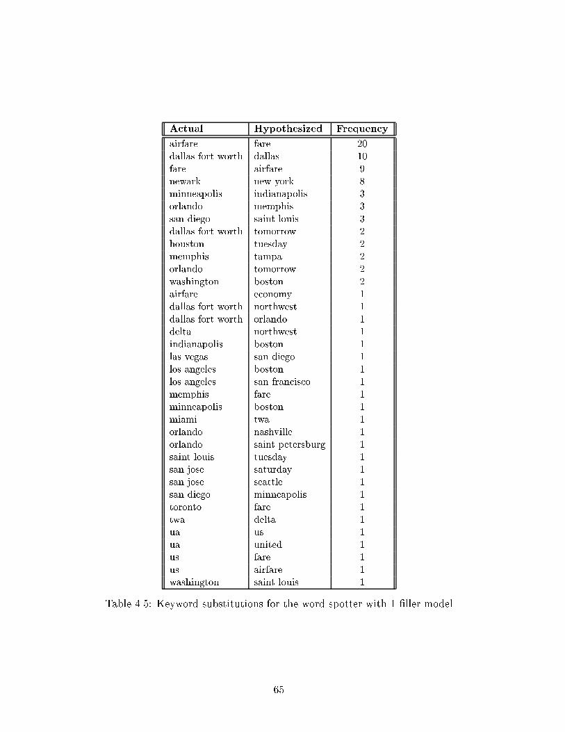
Actual Hypothesized Frequency
airfare fare 20
dallas fort worth dallas 10
fare airfare 9
newark new york 8
minneapolis indianapolis 3
orlando memphis 3
san diego saint louis 3
dallas fort worth tomorrow 2
houston tuesday 2
memphis tampa 2
orlando tomorrow 2
washington boston 2
airfare economy 1
dallas fort worth northwest 1
dallas fort worth orlando 1
delta northwest 1
indianapolis boston 1
las vegas san diego 1
los angeles boston 1
los angeles san francisco 1
memphis fare 1
minneapolis boston 1
miami twa 1
orlando nashville 1
orlando saint petersburg 1
saint louis tuesday 1
san jose saturday 1
san jose seattle 1
san diego minneapolis 1
toronto fare 1
twa delta 1
ua us 1
ua united 1
us fare 1
us airfare 1
washington saint louis 1
Table 4.5: Keyword substitutions for the word spotter with 1 �ller model
65

tables of one or more of the previously discussed word spotters. It is interesting to note
that only 13.2% of the substitutions are across wordclass. This �gure, when combined
with all previous across-class substitution results, leads to the reinforcement of the
conclusion that language modeling does not play a major role in the creation of the
substitution pairs. The most interesting error for this system was the complete failure
in detecting nineteen keywords. Of these keywords, eight were not hypothesized at
all by the word spotter, while the other ten demonstrated between one and nine pre-
normalized insertions (approximately 0.5 to 4.5 when normalized for time). There
does not seem to exist any pattern in the missed instances of these keywords. Most of
them are long words, a characteristic that should have worked to their bene�t. The
keywords \indianapolis," and \minneapolis" are very similar acoustically, but while
the former achieved good performance, the latter was not detected at all. The same
observation can be made for the keyword pair \new york" and \newark". In checking
the frequency of appearance of these keywords in the training set (Table 2.3), we
discovered that it is relatively low for all of them. For instance, \newark" has about
one-third the number of training tokens that \new york" has. Therefore, it should
be relatively easy for a string composed of multiple instances of the single �ller to
out-score the keyword. Indeed, comparing the bigram score for these keywords to the
composite bigram score of the hypothesized strings of C1's, we see that the strings are
favored signi�cantly. Once again, there is a need to add some weight to the keyword
hypotheses, in order to out-score the very general �ller model.
4.4.4 Conclusions
The use of only one general �ller model for background representation resulted in a
sharp drop in performance, as measured by the FOM. A large number of keywords
were completely missed, most probably due to their low bigram model probabilities.
There appears to be a lot of room for improvement, which could possibly be achieved
by manipulating the language model to favor the keywords more than it currently
does. The computation time for the Viterbi search decreased by 46.8% compared
to the fastest spotter discussed so far (word spotter with twelve �ller models). The
66

gain in computation though is overshadowed by the poor word spotting performance,
making this con�guration overall not satisfactory.
4.5 Summary
In this chapter, we investigated the tradeo� between FOM performance and com-
putation time for word spotting systems that use only a few general �ller models.
A steady drop in performance was observed as the number of �ller models was de-
creased from �fty-seven to eighteen, to twelve, and to one. The word spotter with
eighteen �llers achieved performance approaching that of the spotter with context-
independent phones for �llers. The computation time required for the Viterbi stage
decreased steadily with the number of �llers. The classi�cation time increased for the
spotter with 18 �ller models and decreased for the other two systems. As a result, the
overall computation time required by these word spotters did not steadily decrease
as fewer �ller models were used. The performance and computation time for these
systems are shown in comparison to those of the context-independent phone spotter
in Figure 4-9.
1 Filler 12 Fillers 18 Fillers 57 Fillers0
10
20
30
40
50
60
70
80
90
0
2
4
6
8
10
12
14
16
FO
M (
%)
Act
ual C
ompu
tatio
n T
ime
(sec
onds
)FOM Computation Time
Figure 4-9: FOM and computation time measurements for the spotters with 18, 12,and 1 �ller models. The corresponding measurements for the CI spotter are shownfor comparison.
67

Chapter 5
Word-Dependent Models for
Keywords
All the word spotting systems discussed so far have been using context-independent
models for keyword modeling. It has been shown in the literature that the use of
context-dependent models almost always provides better recognition results. In this
chapter, we discuss the bene�ts and shortcomings of using context dependency in
the modeling of the keywords used for word spotting, and present some results. We
have shown that signi�cant improvements in performance can be achieved, but at a
corresponding increase in computation time.
5.1 Word-Dependent Models
We concentrated on creating word-dependent (WD) models for the keywords only,
since it would enable us to compare word spotters with di�erent background repre-
sentations. Due to system limitations, some keywords could only be modeled as a
combination of word-dependent and context-independent models. The total number
of models for the LVCSR spotter, as well as for the system with context-independent
phones as �llers, now reached 520, with 463 of them being word-dependent. The
68

context-independent phones were trained from all non-keyword tokens, with the addi-
tion of the training instances of phones that appear more than once within a keyword,
as explained above.
Another issue that had to be taken into consideration was the amount of train-
ing data available for the word dependent models. Very frequent keywords such as
\boston" or \denver" that occur over 1000 times in the training set naturally have
su�cient data to train word-dependent models. That is not the case for keywords
such as \tampa" and \montreal" that have less than 50 training instances. A solu-
tion to this problem was to linearly interpolate between the scores received by the
word-dependent models and their respective context-independent models as shown in
Equation 5.1.
� =Count
Count+K
Score = (�)ScoreWD + (1� �)ScoreCI (5.1)
where,
Count : The frequency of the word-dependent model in the training set.
K : A smoothing constant to be decided upon during training.
� : The interpolation parameter.
If the number of training tokens for a word-dependent model is high compared to K,
then � will approach 1 and the �nal score will be that of the word-dependent model.
On the other hand, if there is not su�cient data for the word dependent model, then
� will become very small and the score will approach that of the context-independent
model, which is better trained.
The only remaining issue was how to estimate the best value for the smoothing
parameter K. In a large vocabulary speech recognition experiment, we would adjust
this parameter until we achieved the highest possible word accuracy on a development
set. Since our interest was in word spotting performance, we decided to select the
smoothing parameter value that maximized the FOM. The training procedure was
69

slightly modi�ed to enable the estimation of the appropriate value for K. According
to the new procedure, a few training iterations were performed �rst with K set to
zero to allow for the word transition penalty, the segment transition weight, and the
pronunciation arc-weights to acquire their appropriate values. Then, a sequence of
word spotting experiments were conducted on the �rst development set (dev1), with
varying values for the smoothing parameter, in order to collect enough data for the
generation of a graph of FOM versus K. Training was completed with a few more
iterations, in which the value of K that corresponds to a maximum in the graph was
used. The evaluation was done on a second development set (dev2), in order to avoid
over-training on dev1.
We only built two word spotting systems that use word-dependent models, because
they require an excessive amount of time for training and testing. As mentioned in
previous sections, classi�cation is a very time consuming process in the version of
SUMMIT that was used for these experiments. Therefore, the addition of a large
number of word-dependent models made further experimentation prohibitive. The
two systems that were developed are the LVCSR spotter, and the spotter with context-
independent phones as �llers.
5.2 LVCSR Spotter with WD Models for the Key-
words
We begin our study on the e�ects of the introduction of context-dependency in acous-
tic modeling by rebuilding the LVCSR word spotter, and comparing its performance
to that of the corresponding system that uses only context-independent models.
5.2.1 Description of System and Results
Only minor changes had to be made to the LVCSR system presented in Section 3.1,
in order to incorporate the word-dependent models. The arcs for the keywords in the
pronunciation network had to be relabeled in order to re ect the word dependency.
70

The maximum number of mixture Gaussians that was used for modeling both the
context-independent phones and the word-dependent phones was again twenty-�ve.
During classi�cation, each segment received scores for both types of models. Then the
appropriate score pairs were combined according to Equation 5.1, and the resulting
�nal score was reassigned to the word-dependent model. The bigram language model
was una�ected by the above changes, since they occurred only within words.
After the �rst set of weight iterations was completed, we generated the curve of
FOM versus the smoothing parameter, which is shown in Figure 5-1. The two highest
500 1000 1500 2000 2500 3000 3500 400075
80
85
90
95
100
smoothing parameter, K
FO
M
Figure 5-1: Graph of FOM versus the smoothing parameterK, for the LVCSR spotterwith word-dependent models.
FOM values in this graph are at approximately 1500 and 2500. As discussed earlier,
the larger the value of the smoothing parameter, the smaller the contribution of the
word-dependent models to the �nal score. Given that the maximum frequency of any
keyword in the training set is about 1300, it seemed logical to select the lower peak.
Then, in the case of the most frequent words, the two sets of models contribute equally
to the �nal score, whereas for the more infrequent words the context-independent
score carries more weight. Using the smoothing value of 1500, we then performed a
few more weight iterations, in order to readjust the arc, segment, and word transition
weights.
71

The �gure of merit for this word spotter was measured at 91.4%, approximately
1.6% in absolute value above that of the LVCSR system with only context-independent
phone models. The ROC curve for the word spotter is shown in Figure 5-2.
0 1 2 3 4 5 6 7 8 9 100
0.1
0.2
0.3
0.4
0.5
0.6
0.7
0.8
0.9
1
False Alarms/Keyword/Hour
Pd
Figure 5-2: Probability of detection as a function of the false alarm rate for theLVCSR spotter with word-dependent models for the keywords.
The ROC curves for the individual keywords are shown in Figure 5-3.
5.2.2 Comparison to LVCSR Spotter without WD Models
Comparing the performance curve of this spotter to that of the LVCSR spotter with-
out WD models (Figure 3-3) leads to several interesting observations. The probability
of detection for the former is a lot higher around zero fa/k/h, and rises over 90% by
the second fa/k/h, compared to the fourth for the latter. That means that at low
false alarm rates the word spotter with word-dependent models performs much better
than the spotter with only context-independent models. At high false alarm rates the
performance of the two is very close. Therefore, the gain in the system's FOM is
mostly due to better spotting performance at low false alarm rates.
Contrasting the individual keyword performances now, we see that nineteen of the
keywords demonstrated improvement, fourteen performed slightly worse, and the rest
72

0 5 100
0.5
1AIRFARE
0 5 100
0.5
1AMERICAN
0 5 100
0.5
1ATLANTA
0 5 100
0.5
1BALT/RE
0 5 100
0.5
1BOSTON
0 5 100
0.5
1CHAR/TE
0 5 100
0.5
1CHICAGO
0 5 100
0.5
1CIN/ATI
0 5 100
0.5
1CLE/LAND
0 5 100
0.5
1CON/TAL
0 5 100
0.5
1DALLAS
0 5 100
0.5
1DA. FO. WO.
0 5 100
0.5
1DELTA
0 5 100
0.5
1DENVER
0 5 100
0.5
1DETROIT
0 5 100
0.5
1EASTERN
0 5 100
0.5
1ECONOMY
0 5 100
0.5
1FARE
0 5 100
0.5
1FIR. CLASS
0 5 100
0.5
1FRIDAY
0 5 100
0.5
1HOUSTON
0 5 100
0.5
1IND/POLIS
0 5 100
0.5
1KAN. CITY
0 5 100
0.5
1L. VEGAS
0 5 100
0.5
1L. ANG.
0 5 100
0.5
1MEMPHIS
0 5 100
0.5
1MIAMI
0 5 100
0.5
1MILW/KEE
0 5 100
0.5
1MIN/POLIS
0 5 100
0.5
1MONDAY
0 5 100
0.5
1MONTREAL
0 5 100
0.5
1NAS/LE
0 5 100
0.5
1N. YORK
0 5 100
0.5
1NEWARK
0 5 100
0.5
1NOR/EST
0 5 100
0.5
1OAKLAND
0 5 100
0.5
1ORLANDO
0 5 100
0.5
1PHIL/PHIA
0 5 100
0.5
1PHOENIX
0 5 100
0.5
1PIT/BGH
0 5 100
0.5
1R. TRIP
0 5 100
0.5
1S. LOUIS
0 5 100
0.5
1S. PET/RG
0 5 100
0.5
1S. L. CITY
0 5 100
0.5
1S. DIEGO
0 5 100
0.5
1S. FRA/SCO
0 5 100
0.5
1S. JOSE
0 5 100
0.5
1SATURDAY
0 5 100
0.5
1SEATTLE
0 5 100
0.5
1SUNDAY
0 5 100
0.5
1THU/DAY
0 5 100
0.5
1TOM/ROW
0 5 100
0.5
1TUESDAY
0 5 100
0.5
1TWA
0 5 100
0.5
1TAMPA
0 5 100
0.5
1TORONTO
0 5 100
0.5
1UA
0 5 100
0.5
1US
0 5 100
0.5
1UNITED
0 5 100
0.5
1WASH/TON
0 5 100
0.5
1WED/DAY
Figure 5-3: Individual ROC curves for the LVCSR spotter with word-dependentmodels for the keywords.
73

did not change signi�cantly. The number of misses decreased only slightly from 154
to 147, but the number of substitutions dropped drastically from 72 to 52, as shown in
Table 5.1. A large number of substitutions has been avoided with the better acoustic
Actual Hypothesized Frequency
newark new york 13
airfare fare 9
tampa atlanta 5
new york newark 4
minneapolis indianapolis 2
sunday saturday 2
ua us 2
airfare us 1
atlanta toronto 1
economy baltimore 1
fare airfare 1
chicago atlanta 1
indianapolis minneapolis 1
miami montreal 1
monday sunday 1
orlando atlanta 1
orlando saturday 1
san jose saturday 1
tampa toronto 1
thursday eastern 1
thursday wednesday 1
tomorrow houston 1
Table 5.1: Keyword substitutions for the LVCSR spotter with word-dependent mod-els.
modeling of the keywords. The majority of the remaining substitution errors are due
to keywords that are extremely acoustically similar, such as \fare" and \airfare," and
\new york" and \newark," which account for 42% of this spotter's substitutions.
We close this survey on the e�ects of incorporating word-dependent models for the
keywords in the LVCSR spotter by providing some timing data. The classi�cation
stage for this system required approximately 5.7 times more computation than it
did for the LVCSR spotter without word-dependent models. The computation time
for the Viterbi stage remained relatively stable. Based on these results, it appears
that incorporating word-dependent models in the LVCSR word spotter has a more
74

negative e�ect on computation time than a positive e�ect on performance.
5.3 CI Spotter with WDModels for the Keywords
In the previous section, we showed that the introduction of word-dependent models in
the LVCSR word spotter resulted in a considerable improvement in performance. We
continue our study on the e�ects of more precise acoustic modeling for the keywords,
by rebuilding the system with context-independent phones as �llers.
5.3.1 Description of System and Results
The modi�cations that were made to the CI word spotter described in Section 3.2,
in order to incorporate the word-dependent models, are similar to those discussed
previously for the LVCSR spotter. The plot of FOM versus the smoothing parameter
was constructed again, after the �rst set of weight iterations was completed, and is
shown in Figure 5-4.
500 1000 1500 2000 2500 3000 3500 400075
80
85
90
95
100
smoothing parameter, K
FO
M
Figure 5-4: Graph of FOM versus the smoothing parameter K, for the spotter withcontext-independent phones as �llers.
75

This curve has two local maxima, one at approximately 1250, and one at about
2750. For the reasons analyzed in the previous section, we selected the lower peak
at 1250 to be the smoothing value in the calculation of the interpolated score for the
word-dependent models.
The improvement in performance for this word spotter was much larger than that
for the LVCSR spotter. The FOM was calculated to be 86.7%, an increase of 4.8%
in absolute value compared to the spotter without word-dependent models. The
ROC curve for the word spotter is shown in Figure 5-5, and the ROC curves for the
individual keywords are shown in Figure 5-6.
0 1 2 3 4 5 6 7 8 9 100
0.1
0.2
0.3
0.4
0.5
0.6
0.7
0.8
0.9
1
False Alarms/Keyword/Hour
Pd
Figure 5-5: Probability of detection as a function of the false alarm rate for the CIspotter with word-dependent models for the keywords.
5.3.2 Comparison to CI Spotter without WD Models
We will begin the comparison between this system and its counterpart without word-
dependent models by examining their respective ROC curves. The probability of
detection for this word spotter around zero fa/k/h is over 10% higher, but rises at
a smaller rate up to the second false alarm. The two curves have approximately the
same slope after the second fa/k/h, only the probability of detection for this system
76
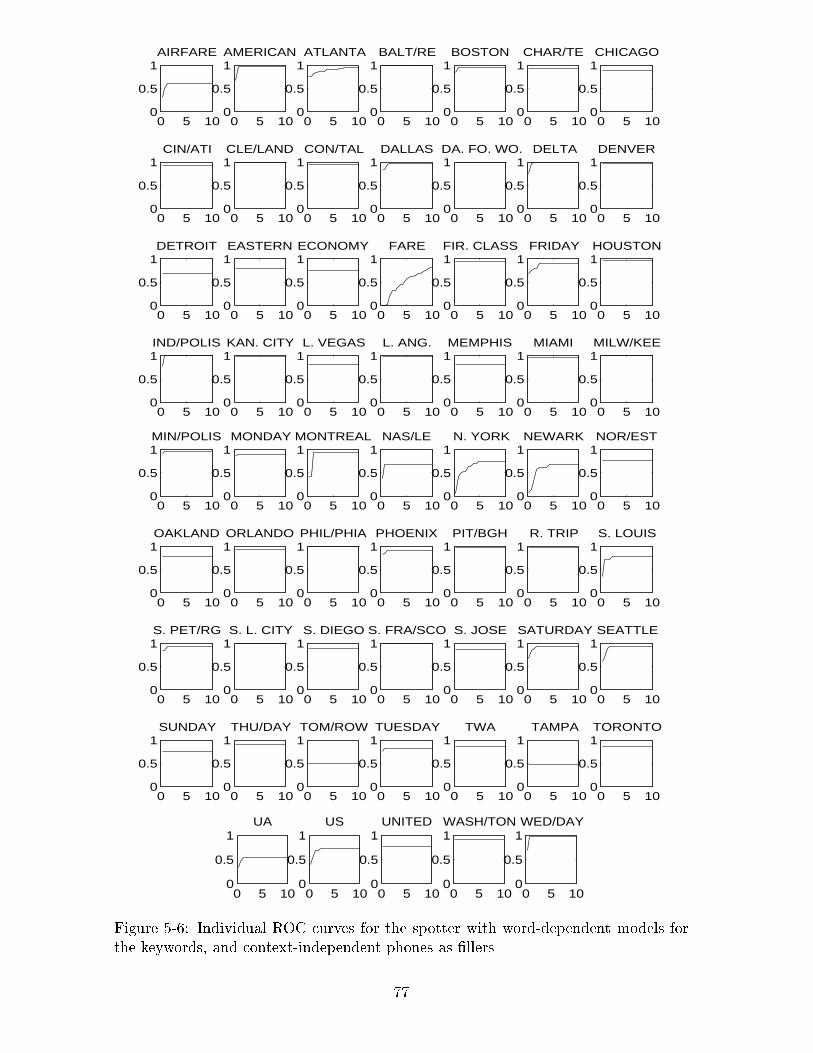
0 5 100
0.5
1AIRFARE
0 5 100
0.5
1AMERICAN
0 5 100
0.5
1ATLANTA
0 5 100
0.5
1BALT/RE
0 5 100
0.5
1BOSTON
0 5 100
0.5
1CHAR/TE
0 5 100
0.5
1CHICAGO
0 5 100
0.5
1CIN/ATI
0 5 100
0.5
1CLE/LAND
0 5 100
0.5
1CON/TAL
0 5 100
0.5
1DALLAS
0 5 100
0.5
1DA. FO. WO.
0 5 100
0.5
1DELTA
0 5 100
0.5
1DENVER
0 5 100
0.5
1DETROIT
0 5 100
0.5
1EASTERN
0 5 100
0.5
1ECONOMY
0 5 100
0.5
1FARE
0 5 100
0.5
1FIR. CLASS
0 5 100
0.5
1FRIDAY
0 5 100
0.5
1HOUSTON
0 5 100
0.5
1IND/POLIS
0 5 100
0.5
1KAN. CITY
0 5 100
0.5
1L. VEGAS
0 5 100
0.5
1L. ANG.
0 5 100
0.5
1MEMPHIS
0 5 100
0.5
1MIAMI
0 5 100
0.5
1MILW/KEE
0 5 100
0.5
1MIN/POLIS
0 5 100
0.5
1MONDAY
0 5 100
0.5
1MONTREAL
0 5 100
0.5
1NAS/LE
0 5 100
0.5
1N. YORK
0 5 100
0.5
1NEWARK
0 5 100
0.5
1NOR/EST
0 5 100
0.5
1OAKLAND
0 5 100
0.5
1ORLANDO
0 5 100
0.5
1PHIL/PHIA
0 5 100
0.5
1PHOENIX
0 5 100
0.5
1PIT/BGH
0 5 100
0.5
1R. TRIP
0 5 100
0.5
1S. LOUIS
0 5 100
0.5
1S. PET/RG
0 5 100
0.5
1S. L. CITY
0 5 100
0.5
1S. DIEGO
0 5 100
0.5
1S. FRA/SCO
0 5 100
0.5
1S. JOSE
0 5 100
0.5
1SATURDAY
0 5 100
0.5
1SEATTLE
0 5 100
0.5
1SUNDAY
0 5 100
0.5
1THU/DAY
0 5 100
0.5
1TOM/ROW
0 5 100
0.5
1TUESDAY
0 5 100
0.5
1TWA
0 5 100
0.5
1TAMPA
0 5 100
0.5
1TORONTO
0 5 100
0.5
1UA
0 5 100
0.5
1US
0 5 100
0.5
1UNITED
0 5 100
0.5
1WASH/TON
0 5 100
0.5
1WED/DAY
Figure 5-6: Individual ROC curves for the spotter with word-dependent models forthe keywords, and context-independent phones as �llers.
77

is consistently around 5% higher. Thus, unlike what was observed for the LVCSR
spotter, there is a gain in the probability of detection for all false alarm rates up to
ten fa/k/h. The highest gain is achieved again at very low false alarm rates.
In comparing the individual ROC curves for the keywords, it is observed that
forty-�ve of the keywords performed better, three slightly worse, and the rest approx-
imately the same. The number of missed keywords was 220, out of which forty-eight
were due to substitution errors. These results indicate a vast improvement over
the corresponding system without word-dependent models, which demonstrated 321
misses and sixty-seven substitutions. The substitution pairs are shown in Table 5.2.
Actual Hypothesized Frequency
airfare fare 9
new york newark 6
tampa atlanta 6
us fare 4
pittsburgh saint petersburg 2
us ua 2
american newark 1
boston atlanta 1
chicago saint louis 1
denver fare 1
minneapolis indianapolis 1
newark ua 1
new york us 1
orlando atlanta 1
phoenix saint louis 1
tampa cleveland 1
ua miami 1
us saint louis 1
Table 5.2: Keyword substitutions for the spotter with word-dependent models for thekeywords, and context-independent phones as �llers.
Comparing these substitution pairs to those in Table 3.2, we observe that while the
keyword \new york" was substituted eight times for the keyword \newark" in that
system, it was not substituted even once here. On the other hand, the number
of substitutions of \new york" by \newark" increased from three to six. The net
e�ect was a decrease in the frequency with which the two words were confused for
78

each other. Some of the most frequent pairs in Table 3.2, such as \airfare" and
\fare," \tampa" and \atlanta" demonstrated even more substitutions in this system.
This indicates that for very acoustically similar word-pairs, the introduction of word-
dependent acoustic models does not always result in less confusion between them.
The bene�t of using word-dependent models is mainly evident in the large reduction
of single substitution errors between keywords that are acoustically dissimilar.
In the error analysis section for the spotter with context-independent phones as
�llers, the error resulting from the hypothesis of strings of phone-words in the place of
the actual keywords was discussed in detail. A similar analysis was performed for this
system, and lead to the conclusion that the more explicit modeling of the keywords
signi�cantly reduced the frequency of this type of substitution. The large composite
bigram score that caused this error was o�set by a higher acoustic score, leading
to the correct hypothesis of the keyword. Speci�cally, for the keyword \fare" the
number of misses due to this error dropped from thirty-four to twelve, for \nashville"
from �fteen to eight, and for \tomorrow" from eleven to seven. Similar results were
obtained for many of the other keywords.
We will conclude the comparison between the two spotters with a few observations
regarding computation time. Similarly to the LVCSR spotter, the computation time
required by the classi�cation stage of this system was approximately 5.6 times longer
than that of the corresponding spotter without word-dependent models. The compu-
tation time attributed to the Viterbi search was unchanged. In this case, it is hard
to decide whether there is a net bene�t or loss. The gain of 4.8% in absolute FOM is
very signi�cant, but it is greatly diminished by the �ve-fold increase in computation
time.
5.4 Summary
In this chapter we investigated the e�ects of word-dependent modeling in word spot-
ting performance and the required computation time. Only the keywords were mod-
eled by word-dependent models, so that comparison between spotters with di�erent
79

background representations would be feasible. Both of the systems that were devel-
oped demonstrated an improvement in performance as measured by the FOM. The
number of substitutions between acoustically similar keywords decreased substan-
tially, as was expected. The number of keyword misses, due to strings of phone-words
being hypothesized in place of the keywords, also decreased considerably for the spot-
ter with context-independent phones as �llers. Unfortunately, the computation time
required for either of these word spotters increased by approximately a factor of �ve,
thus signi�cantly impacting the performance gain. Figure 5-7 summarizes the FOM
and overall actual computation time results for the LVCSR and CI systems.
LVCSR LVCSR + WD CI Fillers CI Fillers + WD0
10
20
30
40
50
60
70
80
90
100
0
10
20
30
40
50
60
70
80
90
FO
M (
%)
Act
ual C
ompu
tatio
n T
ime
(sec
onds
)
FOM Computation Time
Figure 5-7: FOM and computation time measurements for the LVCSR and CI spotterswith and without word-dependent models.
80
Chapter 6
Summary and Improvements
In the previous three chapters we described word spotting systems with a variety
of background representations that range from whole words to a single very general
model. We also examined the e�ects on word spotting performance and computa-
tion time of incorporating word-dependent models for the keywords. In the following
sections, we summarize the results of all word spotting experiments and propose an
iterative training procedure that improves performance without a�ecting the com-
putation time. We conclude the study with a brief discussion of future research
directions and possible applications of the developed word spotting systems.
6.1 Summary of Results
6.1.1 FOM Performance
The measure we used to evaluate the performance of the word spotters was the Figure
of Merit, which was de�ned as the average probability of detection over the �rst ten
false alarms per keyword per hour. The performance of all word spotters developed
for this study, as measured by the FOM, is shown in Table 6.1. The results for
the systems that used only context-independent phones for keyword modeling are
shown in the �rst column. The second column lists the performance of the systems
81

Word spotter CI models WD models
LVCSR 89.8% 91.4%CI �llers 81.8% 86.7%18 �llers 79.2% -12 �llers 76.5% -1 �ller 61.4% -
Table 6.1: FOM performance results for all developed word spotting systems.
that used a combination of context-independent and word-dependent models for the
keywords. As explained in Chapter 5, only two systems using word-dependent models
were designed, since their training and testing were very computationally intensive.
There is clearly a correlation between the degree of explicitness in background
modeling and word spotting performance as measured by the FOM. The LVCSR
utilizes the most detailed �ller models, i.e., whole words, and achieves the highest
performance of all spotters. As �ller models become fewer and more general, the
FOM decreases monotonically.
The LVCSR system outperforms the spotter that uses only a single �ller model
by almost thirty percent in absolute FOM value. The largest portion of this perfor-
mance gain can be attributed to the use of more re�ned acoustic models for the back-
ground. An increase of 20.4% in the FOM is achieved when the number of �ller mod-
els is increased from one general acoustic model to �fty-seven context-independent
phones. This result suggests that the use of more re�ned phone representations,
such as context-dependent phones, could further improve the FOM. The remaining
8% gain in performance is achieved by incorporating domain speci�c knowledge, i.e.,
using models of all non-keyword words as �llers. This further improvement can be
attributed to two factors. First, by explicitly modeling all words in the domain we
impose a tighter constraint on the possible transcriptions of each utterance. The �ller
words for the LVCSR are modeled as concatenations of context-independent phones.
When hypothesized they consist of multiple segments. In contrast, the �llers for
the spotters with one, twelve, eighteen and �fty-seven �ller models are hypothesized
as single segment \words." Consequently, the output transcription of these systems
82

generally consists of a larger number of words than the corresponding transcription
of the LVCSR system. The second factor contributing to the performance gain is
the bigram language model. Although a bigram component is incorporated in all
systems, its bene�ts become most evident for the LVCSR spotter. For instance, the
probability that the current word is a city name, given that the previously hypothe-
sized word was \from," is much higher than if the previous word was the single �ller
model \C1". In conclusion, the largest gain in FOM, with respect to the spotter with
a single �ller model, was achieved with increasingly more explicit acoustic modeling
of the background. The use of whole words as �llers resulted in a more constrained
search space and a more e�ective bigram component. The spotter with whole words as
�llers achieved an additional, signi�cant gain in word spotting performance, without
requiring any further improvement in the acoustic modeling of the segments.
The introduction of word-dependent models for the keywords resulted in an im-
provement in the performance of the systems that were developed. Both spotters
demonstrated a signi�cant reduction in the number of keyword substitutions. The
main source of improvement for the CI spotter was the elimination of a large num-
ber of errors caused by the substitution of keywords by strings of phone-words. The
word-dependent models for the keywords received a higher composite acoustic match
score than the corresponding context-independent models. The higher acoustic score
o�set the large composite bigram score of the underlying phone-word strings in many
instances, resulting in the correct hypothesis of the keyword. This type of error did
not occur for the LVCSR spotter, which explains why it demonstrated signi�cantly
smaller improvement in performance than the CI spotter.
In conclusion, we have shown that word spotting performance as measured by the
FOM can be improved upon by (1) using more re�ned acoustic models as �llers, (2)
explicitly modeling all words in the domain of interest, and (3) using more re�ned
acoustic models for the keywords. By using word-dependent models for the keywords
and context-independent phones as �llers, we managed to achieve FOM performance
very close to that of the LVCSR spotter.
83

6.1.2 Computation Time
In this section we present measurements of the computation time required by the in-
dividual word spotters. The method that was used for the collection of these measure-
ments was described in Section 2.5.2. The average computation time per utterance
in seconds is shown in Table 6.2. Both the actual and elapsed time measurements are
CI models WD modelsWord spotter Stage actual elapsed actual elapsed
classi�cation 13.01 13.84 73.88 75.2LVCSR viterbi 7.50 8.52 8.31 17.95
total 20.63 22.48 82.3 93.99classi�cation 12.85 12.9 71.35 71.75
CI �llers viterbi 1.04 1.12 0.96 1.37total 14.01 14.14 72.43 73.24classi�cation 13.81 13.86
18 �llers viterbi 0.63 0.67total 14.56 14.65classi�cation 12.74 12.75
12 �llers viterbi 0.64 0.70total 13.50 13.57classi�cation 10.73 10.92
1 �ller viterbi 0.33 0.33total 11.18 11.37
Table 6.2: Computation time results for all developed word spotting systems.
presented. The elapsed time demonstrated a lot of uctuation between consecutive
timing experiments under the same word spotting conditions. The actual time proved
more stable and was therefore used for the comparison between the word spotting sys-
tems. For every spotter we measured the computation time required for the principal
component rotation, classi�cation, and Viterbi stages of recognition. The �rst stage,
where the vectors of segment measurements are multiplied by a rotation matrix, had
the same average duration of 0.12 seconds for all systems. This amount is included in
the total computation time measurements shown in Table 6.2. The timing results are
not guaranteed to be very precise, so the focus of the comparison will be on general
trends rather than exact measurements.
84
The average computation time for the Viterbi stage decreases as the number of
�ller models was reduced from 2462 for the LVCSR spotter to a single general model.
The only inconsistency to this result was the very small increase in computation ob-
served when the number of �ller models is decreased from eighteen to twelve. The
reduction of the vocabulary size by six words should not signi�cantly a�ect the re-
quired computation time for the search. The most probable explanation for this
inconsistency is that it is a result of the variability in the timing procedure that was
used. The same relation between the Viterbi computation time and the number of
�ller models is observed for the word spotters that use word-dependent models for
the keywords.
The classi�cation times follow a similar trend, but a slightly more in depth analysis
is required in order to fully comprehend their behavior. All the systems developed use
at least �fty-seven acoustic models, and each model is a mixture of up to twenty-�ve
diagonal Gaussians. The LVCSR spotter and the spotter with context-independent
phones as �llers use exactly �fty-seven acoustic models. The word spotters with gen-
eral �llers have an additional number of models equal to their respective number of
�ller models. With these facts in mind, we would expect that the systems with general
�ller models would all have longer classi�cation stages than the systems using whole
words, or context-independent phones as �llers. That is not the case though, as is
evident from the results in Table 6.2. More careful examination of the classi�cation
algorithm leads to the conclusion that the total number of mixture Gaussians, rather
than the total number of models, controls the amount of computation required for this
stage. The spotter with eighteen �ller models had the highest number of mixtures and
the longest classi�cation stage. The LVCSR, CI �ller, and twelve �ller systems had
approximately the same number of mixture Gaussians, and required approximately
the same amount of computation time. Finally, the system with a single �ller model
had a signi�cantly smaller number of mixtures, and also a signi�cantly shorter clas-
si�cation stage compared to any other spotter. The fact that some of these systems
have more models but fewer mixtures than others is easily explained if we consider
the training method that was used in their development. The LVCSR and the spotter
85

with context-independent phones for �llers trained their �fty-seven acoustic models
on all data. Thus, there were enough training tokens for almost all of the models to be
represented by mixtures of the upper-bound of twenty-�ve Gaussians. The spotters
with more general �ller models used only the keyword data to train their context-
independent phones, and the rest of the data to train the �ller models. As a result,
many of the context-independent phones for these systems were modeled by mixtures
of fewer than twenty-�ve diagonal Gaussians. Thus, the context-independent phones
for these systems have a smaller total number of mixtures than the corresponding
phones for the LVCSR and CI spotters. Depending on the number of general models
used by each system, a classi�cation time above or below the mark set by the LVCSR
and CI spotters is achieved.
The introduction of word-dependent modeling had an enormous e�ect on the
classi�cation time for both the LVCSR and the spotter with context-independent
phones as �llers. Both spotters required slightly over 5.5 times more computation
time for the classi�cation stage, a result that is easily justi�ed if we consider the
increase in the number of acoustic models from �fty-seven to 520. Thus, the gain
in performance achieved with these systems is outweighed by their very long average
computation times.
A summary of the performance of all word spotting systems that were developed
for this study is graphically presented in Figure 6-1. For each system, the leftmost
bar corresponds to FOM performance and the rightmost to actual computation time.
The computation required in the principle component stage is omitted since it is the
same for all systems.
As we expected, there is a clear tradeo� between word spotting performance as
measured by the FOM, and the computation time required for spotting. More ex-
plicit modeling of the background results in higher performance, but also requires
more computation. The advantages of a smaller set of �llers are less computation
time and more exibility, in the sense that word spotting in a new domain would
require less training data for language and acoustic modeling. An acceptable com-
promise between FOM performance and computation time seems to be the spotter
86

1 12 18 CI CI + WD LVCSR LVCSR+ WD
0
10
20
30
40
50
60
70
80
90
100
0
10
20
30
40
50
60
70
80
90F
OM
(%
)
Act
ual C
ompu
tatio
n T
ime
(sec
onds
)
FOMClassification
Viterbi
Figure 6-1: FOM and computation time measurements for the all developed wordspotters.
with context-independent phones as �llers. It achieves over 80% FOM, and provides
signi�cant savings in computation time compared to the LVCSR spotter.
The use of word-dependent models for the keywords clearly improves the FOM,
but unfortunately also results in a very large increase in computation. As we have
already explained, the increase in computation is due to the classi�cation algorithmwe
used, which computes an acoustic match score for all models and all segments before
the search is initiated. A classi�cation algorithm that would compute acoustic scores
upon demand during the search would save a lot of computation time, and would make
word-dependent or context-dependent models more attractive. The CI spotter with
word-dependent models for the keywords illustrates the bene�ts of introducing such
re�ned acoustic models into word spotting systems. It achieves an FOM performance
very close to that of the LVCSR spotter, without using any explicit knowledge of the
domain's vocabulary.
This section summarizes the results of our study on out-of-vocabulary word model-
ing for word spotting systems. In the next section we discuss an experimental method
87

that provides variable amounts of gain in FOM performance for all spotters, without
a�ecting their computation time requirements.
6.2 Improving Performance with Keyword-Speci�c
Word-Boosts
In this section we present an iterative process which results in signi�cant improve-
ment in the performance of some of the developed spotters, without a�ecting their
required computation times. The main source of error for the word spotters with
context-independent phones or more general acoustic models as �llers is the substi-
tution of keywords by acoustically similar strings of �llers. Careful analysis of these
errors revealed that the majority of them are due to a very large cumulative bigram
transition score for the �ller strings. The decomposition of non-keywords into strings
of �llers resulted in an asymmetry in the amount of data available for keyword versus
�ller training. Any bigram transition between �llers received counts for the language
model from instances generated by numerous words. Thus, in order to balance the
bigram transition scores into keywords with the transitions into �llers, we decided to
add a word-speci�c boost to each keyword. We observed that most of the keywords
that have many missed instances are not inserted very often. This indicated that
trading insertions with misses might be possible, and could potentially lead to a gain
in performance. To that e�ect, we designed an iterative process that attempts to
equalize the number of insertions and deletions for each keyword during spotting, by
adjusting the keyword-speci�c word-boosts. The set we used for this post-training
stage consists of the union of the two development sets, dev1 and dev2. Our choice of
such a large development set was based on the belief that a higher number of keyword
instances would allow better estimation of the appropriate word-boost values. The
FOM was calculated for each iteration in order to measure improvement and also as
an indicator of when to stop iterating.
The process was applied to the three word spotters with general �ller models and
the spotter with context-independent phones as �llers. For all of the above systems the
88

FOM on the new development set increased as the number of insertions approached
the number of deletions for each keyword. The set of word-boosts that resulted in the
highest FOM value was selected, and the boosts were added to the appropriate bigram
transition scores into the keywords. Then, word spotting was performed on the same
test set. The new performance measurements are shown in Table 6.3. We see that
Word spotter FOM without boost FOM with boost
CI �llers 81.8% 84.5%18 �llers 79.2% 82.7%12 �llers 76.5% 82.8%1 �ller 61.4% 62.6%
Table 6.3: Performance improvements resulting from the introduction of keyword-speci�c word-boosts.
the highest gain of 6.3% in absolute FOM was realized by the spotter with twelve
general �ller models, followed by a gain of 3.5% for the spotter with eighteen general
�ller models, and 2.6% for the spotter with context-independent phones as �llers.
The spotter with a single �ller demonstrated only a 1.2% increase in absolute FOM
performance. As expected, the number of missed instances decreased for all systems,
while the number of keyword substitutions by other keywords remained relatively
stable.
We have shown that signi�cant improvement in word spotting performance can
be achieved with a simple, post-training process. The process estimates appropriate
keyword-speci�c boosts, which compensate for the large bigram transition scores of
the �ller models. We believe that even higher gains can be achieved by further re�ning
this process.
89

6.3 Future Work
6.3.1 Improvements and Flexibility
In this study we developed word spotting systems that use background representations
ranging from a single general acoustic model to whole words. We veri�ed that the
LVCSR spotter provides the best performance as measured by the FOM, but also
requires signi�cantly more Viterbi computation time than any of the other spotters.
It is also the least exible system, since knowledge of the full vocabulary is required
in order to build the background representation. A word spotter that demonstrated
FOM performance relatively close to that of the LVCSR was the CI spotter, especially
with the introduction of word-dependent models for the keywords. This system is
more exible than the LVCSR, but requires a large number of keyword instances in
order to e�ciently train the word-dependent models. It also requires a large amount
of computation in the classi�cation stage. Based on these results, future research will
attempt to satisfy the following goals:
� Utilize a faster, more e�cient classi�cation algorithm.
� Evaluate the exibility of the developed word spotting systems within and across
domains.
� Use context-dependent phones both for the keywords and as �llers.
The development of a faster classi�cation algorithm is necessary in order to realize
the bene�ts of the word-dependent models. Furthermore, it will allow the incorpora-
tion of context-dependent phones into the word spotting systems.
We intend to use the developed word spotting systems in a set of experiments
that will evaluate their exibility within and across domains. First, we will moni-
tor the e�ects on performance of adding or subtracting keywords within the ATIS
domain. In these experiments, the acoustic models will remain unchanged and only
the bigram language model will be recomputed. The systems with word-dependent
models will not be rebuilt for this set of experiments. Second, we will measure the
90

FOM performance of these word spotting con�gurations in other domains and with
varying training set sizes.
Context-dependent phones can provide a more re�ned background representa-
tion than context-independent phones. They can also be used in place of the word-
dependent phones, thus easing the requirement for many keyword instances in the
training set. A spotter that will use context-dependent phones for both keyword and
background representation will therefore be rather exible, and will hopefully achieve
performance very close to that of the LVCSR spotter.
6.3.2 Possible Applications
As we discussed in Chapter 1, there is a continuously growing number of word spotting
applications. One of our goals is to incorporate a word spotting systems with few �ller
models as a front-end to the GALAXY [4] system. GALAXY is a distributed system
for providing access and intelligent mediation for on-line information and services via
human-language technology. The current implementation is focused on the travel
domain, and provides air travel, local navigation, and weather information. The
current GALAXY vocabulary consists of nearly 2500 words from all three domains.
The use of such a large vocabulary has a negative e�ect on both recognition time
and on accuracy. Ideally, we would like to know which domain the query refers to in
order to use only the corresponding vocabulary in recognition. That can hopefully
be achieved with a system that spots for a moderate size set of keywords, that are
characteristic of each domain. A probabilistic framework will be constructed, which
will measure the relevance of each domain to the current query. The likelihood of
each domain will be based on the detection of one or more keywords in the current
query, and the results of the domain classi�cation of the previous queries. In the �rst
recognition step, the spotter will return an ordered list of the domains in GALAXY.
In the next step, recognition will be performed starting with the vocabulary of the
most likely domain. If the utterance score falls under a pre-determined threshold, the
vocabulary of the second most likely domain will be used for recognition. This process
will be continued until an acceptable score is returned. We believe that dividing the
91

recognition process into these two steps will result in increased accuracy and savings
in computation time on average. It might also provide a simple way to add more
domains to GALAXY, since only the word spotting component would have to be
rebuilt.
92

Bibliography
[1] B. Chigier. Rejection and keyword spotting algorithms for a directory assistance
city name recognition application. In Proceedings of the 1992 International Con-
ference on Acoustics, Speech and Signal Processing, volume 2, pages 93{96. IEEE,
March 1992.
[2] D. A. Dahl, M. Bates, M. Brown, W.Fisher, K. H. Smith, D. Pallet, C. Pao,
A. Rudnicky, and E. Shriberg. Expanding the scope of the atis task: The atis-
3 corpus. In Proceedings of the Human Language Technology Workshop, pages
43{48. Morgan Kaufmann, March 1994.
[3] J. Glass. Finding acoustic regularities in speech: applications to phonetic recog-
nition. PhD thesis, MIT, 1988.
[4] D. Goddeau, E. Brill, J. Glass, C. Pao, M. Phillips, J. Polifroni, S. Sene�, and
V. Zue. GALAXY: A human-language interface to on-line travel information. In
Proc. International Conference on Spoken Language Processing, volume 2, pages
707{710, Yokohama, Japan, September 1994.
[5] J.J. Godfrey, E.C. Holliman, and J. McDaniel. Switchboard: Telephone speech
corpus for research and development. In Proceedings of the 1992 International
Conference on Acoustics, Speech and Signal Processing. IEEE, March 1992.
[6] P. Jeanrenaude, K. Ng, M. Siu, J.R. Rohlicek, and H. Gish. Phonetic-based word
spotter: various con�gurations and application to event spotting. In Proceedings
of the EUROSPEECH'93, pages 1057{1060, 1993.
93

[7] G.J.F. Jones, J.T. Foote, K. Sparck Jones, and S.J. Young. Video mail retrieval:
the e�ect of word spotting accuracy on precision. In Proceedings of the 1995
International Conference on Acoustics, Speech and Signal Processing, volume 1,
pages 309{312. IEEE, May 1995.
[8] E. Lleida, J.B. Marino, J.Salavedra, A. Bonafonte, E. Monte, and A. Martinez.
Out-of-vocabulary word modelling and rejection for keyword spotting. In Pro-
ceedings of the EUROSPEECH'93, pages 1265{1268, 1993.
[9] MADCOW. Multi-site data collection for a spoken language corpus. In Proceed-
ings of the Fifth DARPA Speech and Natural Language Workshop, pages 7{14.
Morgan Kaufmann, February 1992.
[10] M. Phillips and V. Zue. Automatic discovery of acoustic measurements for pho-
netic classi�cation. In Proc. International Conference on Spoken Language Pro-
cessin, pages 795{798, 1992.
[11] R. Rose. De�nition of subword acoustic units for wordspotting. In Proceedings
of the EUROSPEECH'93, pages 1049{1052, 1993.
[12] S. Sene�. A joint synchrony/mean-rate model of auditory speech processing. In
Proc. J. of Phonetics, volume 16, pages 55{76, January 1988.
[13] R. A. Sukkar and J.G. Wilpon. A two pass classi�er for utterance rejection
in keyword spotting. In Proceedings of the 1993 International Conference on
Acoustics, Speech and Signal Processing, volume 2, pages 451{454. IEEE, April
1993.
[14] M. Weintraub. Keyword-spotting using SRI's DECIPHER large-vocabulary
speech recognition system. In Proceedings of the 1993 International Conference
on Acoustics, Speech and Signal Processing, volume 2, pages 463{466. IEEE,
1993.
[15] L. D. Wilcox and M. A. Bush. Training and search algorithms for an interactive
wordspotting system. In Proceedings of the 1992 International Conference on
94

Acoustics, Speech and Signal Processing, volume 2, pages 97{100. IEEE, March
1992.
[16] J.G. Wilpon, L.R. Rabiner, C. Lee, and E.R. Goldman. Automatic recognition
of keywords in unconstrained speech using hidden markov models. Transactions
on Acoustics, Speech and Signal Processing, 38(11):1870{1878, November 1990.
[17] V. Zue, J. Glass, D. Goodine, M. Phillips, and S. Sene�. The SUMMIT speech
recognition system: phonological modelling and lexical access. In Proceedings of
the 1990 International Conference on Acoustics, Speech and Signal Processing,
pages 49{52. IEEE, 1990.
[18] V. Zue, S. Sene�, J. Polifroni, M. Phillips, C. Pao, D. Goddeau, J. Glass, and
E. Brill. The MIT Atis system: December 1993 progress report. In Proc. ARPA
Spoken Language Technology Meeting, Princeton, March 1994.
95