i

THESIS FOR THE DEGREE OF LICENTIATE OF ENGINEERING

A System Dynamics Analysis of Cost-Recovery

A Study of Rural Minigrid Utilities in Tanzania

ELIAS HARTVIGSSON

Department of Energy and Environment

CHALMERS UNIVERSITY OF TECHNOLOGY

Gothenburg, Sweden 2015

ii

A System Dynamics Analysis of Cost-Recovery

A Study of Rural Minigrid Utilities in Tanzania

ELIAS HARTVIGSSON

© ELIAS HARTVIGSSON, 2015.

Department of Energy and Environment

Chalmers University of Technology

SE-412 96 Gothenburg

Sweden

Telephone + 46 (0)31-772 1000

Cover: Two

[Reproservice]

Gothenburg, Sweden 2015

iii

Abstract

Over one billion people live in poverty around the world. Access to modern energy sources such as electricity is considered important in social and economic development. A number of initiatives have been taken to improve the situation but one billion people still lack access to electricity around the world, most of whom live in rural and inaccessible areas.

One proposed solution to improve electricity access in rural areas is minigrids based on renewable energy sources. Minigrids have been constructed in all parts of the world with various levels of success. A common challenge for the utility’s operating them has been to achieve the ability to cover their own expenses, leading to financial difficulties.

Based on a systemic approach, this work investigates cost-recovery based on a dynamic understanding of the problem. By developing a system dynamics model the problem is analyzed conceptually through a causal loop diagram and mathematically through a stock and flow model. The stock and flow model is then used to investigate the effect different generation and distribution technologies have on cost-recovery.

Through the application of the system dynamics model it is found that construction and planning time together with the cost per connection are both important factors for cost-recovery. When construction and planning times are too long, the utility is not able to handle changes in demand. With a reduced power availability, usage and number of users decrease, creating a negative loop driving down the income. Even though both construction and planning time and cost per connection are found to be important, the results implies that reducing connection cost can have a large impact on cost-recovery, given that the utility has the ability to handle changes in demand.

The work also identifies a possible future area of research where system dynamics modeling is integrated with load modeling and assessments. This could reduce the issues of using a static relationship between electricity and power and thereby possibly yield new insights into the connection between electricity usage, generation source and cost-recovery.

Keywords: rural electrification, minigrid, cost-recovery, system dynamics

iv

Acknowledgement

This work would not had been possible if it wasn’t for the support of all people involved. There are too many people I would like to thank to all be mentioned here. First of all I would like to thank my supervisors: Jimmy Ehnberg, Sverker Molander and Erik Ahlgren. Without your help, guidance and endless patience to answer all of my questions, this work would not had been possible. I also want to send my sincerest thank you to my colleauges and friends in Tanzania: Joseph Ngowi, Erick Haule, Herode Sindano, Morten Van Donk, Remigiusi Mtewele and Inger Lundgren.

I would also like to thank my colleagues at Environmental Systems Analysis that have made me feel at home when ever I came by, and a special thanks to my colleague Helene Ahlborg. Spending day in and day out at Electric Power Engineering, I wouldn’t have enjoyed it half as much as if it wasn’t for my great colleagues, thank you. A special thanks to Oskar Josefsson and David Steen, I don’t think I will have two colleagues like you again.

To all my friends, thank you for being there and sharing both good and bad times. Thank you Sylvain, Dagmara, Mitra, Elena and Gatto for giving me a new perspective on life. And a special thanks to Lukasz for being the best flatemate one can have. Thank you Liv, Maria, Linus, Boris, Hans, Henrik and Tom for all our memories.

Last but not least, a big thanks to my family: Johannes, Mathilda, Hampus, Lars and Lena. Without your love and encouragement I would never have gotten this far.

v

List of Publications that have been produced as part of this work:

I.   Hartvigsson E. Ahlgren E. Ehnberg J. Molander S., Rural Electrification Through Minigrids in Developing Countries: Initial Generation Capacity Effect on Cost-Recovery, International Conference of System Dynamics 2015, Cambdrige Massachusetts

II.   Hartvigsson E. Ehnberg J. Ahlgren E. Molander S., Assessment of Load Profiles in Minigrids: A Case in Tanzania, IEEE UPEC 2015, Staffordshire University

III.   Hartvigsson E. Ahlgren E. Ehnberg J. Molander S., Rural Electrification – A System Dynamics Analysis of Connection cost on User Growth and Cost-Recovery for Minigrids, To be submitted to European Journal of Operational Research

IV.   Ehnberg J. Ahlborg H. Hartvigsson E., Flexible Distribution Design for Dynamic Load Patterns in Micro-grids, Abstract accepted for PES-Africa Conference 2015

7

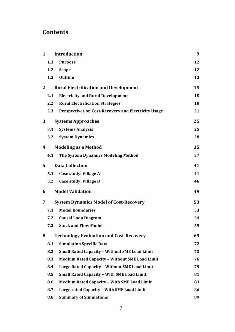
Contents  

1   Introduction   9  1.1   Purpose   12  1.2   Scope   12  1.3   Outline   13  

2   Rural  Electrification  and  Development   15  2.1   Electricity  and  Rural  Development   15  2.2   Rural  Electrification  Strategies   18  2.3   Perspectives  on  Cost-­‐‑Recovery  and  Electricity  Usage   21  

3   Systems  Approaches   25  3.1   Systems  Analysis   25  3.2   System  Dynamics   28  

4   Modeling  as  a  Method   35  4.1   The  System  Dynamics  Modeling  Method   37  

5   Data  Collection   41  5.1   Case  study:  Village  A   41  5.2   Case  study:  Village  B   46  

6   Model  Validation   49  

7   System  Dynamics  Model  of  Cost-­‐‑Recovery   53  7.1   Model  Boundaries   53  7.2   Causal  Loop  Diagram   54  7.3   Stock  and  Flow  Model   59  

8   Technology  Evaluation  and  Cost-­‐‑Recovery   69  8.1   Simulation  Specific  Data   72  8.2   Small  Rated  Capacity  –  Without  SME  Load  Limit   73  8.3   Medium  Rated  Capacity  –  Without  SME  Load  Limit   76  8.4   Large  Rated  Capacity  –  Without  SME  Load  Limit   79  8.5   Small  Rated  Capacity  –  With  SME  Load  Limit   81  8.6   Medium  Rated  Capacity  –  With  SME  Load  Limit   83  8.7   Large  rated  Capacity  –  With  SME  Load  Limit   86  8.8   Summary  of  Simulations   89  

8

9   Discussion  and  Implications   90  

10   Main  Contributions  and  Recommendations  for  Future  Work   94  10.1   Recommendations  for  Future  Work   94  

11   Appendix   96  

12   References   98  

9

1   Introduction

Today 1.2 billion people live in the OECD countries, where access to energy and electricity is abundant and a life without it is almost impossible. The fact that access to cheap and reliable energy is one of the pillars in our current economic welfare is evident, so is the role it has played in our development. However, there are still one billion people living in extreme poverty where a life with access to reliable electricity, sanitation and clean water is no more than a desire (IEA, 2015; UNDP, 2014).

It is not merely a coincidence that the amount of people living without access to electricity, water and sanitation and living under extreme poverty are similar. Without sufficient income households are unable to pay for an electricity connection or the necessary changes needed to be done to the house to allow internal wiring. Similarly, income is a barrier in access to clean water and sanitation facilities when the poor don’t receive access to infrastructure (Bardhan & Mookherjee, 2006). Without access to basic sanitation services, health is reduced, whereby peoples ability to work is reduced. The interactions between different sectors can cause a negative spiral, or a loop, making it very difficult or impossible for individuals to improve their situation without external support (Sachs, 2005).

The interest for electrification and modern energy sources in the global development agenda has seen a rise over the last decades. Academia as well as bilateral and multilateral aid agencies across the globe have increased the emphasis on electricity access (The White House, 2013)1. And the role that access to modern energy sources plays in human development has been emphasized in the United Nations new goals for human development, the Sustainable Development Goals. Even though the previous goals, the Millennium Development Goals, indirectly treated access to modern energy, they didn’t explicitly set up targets for access to modern energy sources as a specific goal in human development and well-being. The new Sustainable Development Goals reassessed the role of access to modern energy and its role in human development.

1 Based on a search through the sciencedirect database that shows an

increase in the amount of scientific publications containing the search terms “africa” and “electrification” starting from the late 90s until 2014.

10

Improving electricity access is considered important in the work of poverty alleviation. Even though access to reliable and cheap energy is vital for improving socio-economic conditions, the actual causality between access to electricity and social and economical development has not been agreed upon. There has been considerable research on the subject but the results have not been conclusive. However, what is agreed upon by both academics and practitioners is that electricity is a prerequisite for development and that it will play a central role in alleviating poverty (Barnes, 2007).

In order to reduce poverty, the OECD countries distributed 134 billion USD in foreign aid in 2013. As a complement to the foreign aid, private capital flows added another 150-250 billion dollars lead by private organizations and foundations such as the Gates Foundation (OECD, 2011). As a result, the amount of people living in absolute poverty has declined from 2.2 billion in 1970 to 1 billion in 2011 while at the same time the amount of people not living in absolute poverty grew from 1.5 billion to 6 billion people (Roser, 2011). The striking increase in improved conditions has come at a great cost on environmental impacts in terms of emissions and land use (Chow, Kopp, & Portney, 2003).

The large private capital flows have indubitable had positive effects on development, but they have also been very volatile (much more so than foreign aid) and have also in some instances focused on corporate profit rather than socio-economic development (Cook, 2011; OECD, 2011). It is clear that the costs to build the necessary infrastructure in developing countries are too large for any single actor and need to be shared amongst both public and private donors (Williams, Jaramillo, Taneja, & Ustun, 2015).

The increase in electricity access has mostly been done using a similar strategy as in the western world, both in terms of technology choice and financial support. This has led to a focus on large centralized generation systems relying on fossil fuels. With the increasing pressure to decrease greenhouse gas emissions, renewable energy sources have seen a large increase in many OECD countries (REN21, 2014).

Due to many factors, the process of constructing electric power infrastructure in developing countries is especially difficult. Developing countries are often characterized by dispersed populations, low income and a large reliance on agriculture. Dispersed populations makes traditional technologies using power lines expensive and the low income and reliance on

11

agriculture means that electricity usage is very low. Furthermore, the predicted large annual economic growth implies that these countries will see large changes in demographics (Watson, 2014). In rural areas, where access to societal services are generally lacking, the choice to improve electricity access for one community might lead it to become more attractive in the immediate surroundings. In fact, the urbanization rate in developing countries is amongst the highest in the world, making it uncertain which areas and communites that will persist (UN, 2014).

As electricity is introduced in rural areas, health clinics can use electricity to store vaccines, sterilize instruments and improve the general safety. Schools can get access to valuable information through the use of information and communication technology and enterprises can improve their operations, or even initiate new businesses, previously not possible.

As developing countries are still constructing their electric power infrastructure, they have an opportunity to prepare their electric infrastructure for future challenges, such as large share of renewable energy sources. To reduce the large costs associated with electric power infrastructure, especially in rural areas, and to work towards a decentralized generation system, small off-grid systems are a possible option. There are different off-grid technologies but when it comes to supplying enough electricity for productive uses, there are less. However, one option is minigrids. Minigrids are small, independent electricity production and distribution systems. Being able to both supply larger electrical loads and in regions where the national electricity grid is not available they have been used all around the world in rural electrification projects.

Even though there are success stories (Schnitzer et al., 2014), one of the largest challenges for minigrids projects is to achieve a financial sustainability. However, even in the successful projects, the utility’s operating the minigrid are struggling to collect enough revenue to expand their system or even replace equipment (Ahlborg & Sjöstedt, 2015; Schnitzer et al., 2014). The financial difficulties have discouraged many entrepreneurs and investors from investing in rural electrification projects. Even though it is very important to safeguard the needs of socio-economical development for the poorest, rural electrification needs to be made more financially attractive.

The interest in cost-recovery, the ability to cover expenses without any external support, is not new. During the 80s The World Bank put a strong

12

emphasizes on cost-recovery and privatization of the electric power systems in developing countries (Mary, 1996). This led to critique that the societal benefits were put aside for corporate profits when the expected benefits did not happen (Cook, 2011). The problem at this time was not just that there was too much emphasizes on cost-recovery, but rather that both the environmental and socio-economic impacts on the local community where set aside. With a holistic approach it could possible to integrate economic performance of the utilities with socio-economical and environmental impacts on the local community.

Research has shown that holistic approaches are important to understand the dynamic and multidisciplinary environment in communities in which rural electrification projects are implemented (Ahlborg, 2015). One way of analyzing complex socio-technical systems is system dynamics. System dynamics is a modeling method to analyze the connection between socio-economic-technical system structure and behavior. By using both conceptual and mathematical modeling system dynamics integrates the perspectives of systems analysis with control theory.

1.1   Purpose

The purpose of this work is to investigate cost-recovery for rural minigrids in developing countries. By developing a system dynamics model, the connection between system structure and behavior can be analyzed both quantitatively and qualitatively. Furthermore, the thesis aim to use the model to investigate the impact of choice on generation and distribution technology and their implementing times on cost-recovery.

1.2   Scope

This work explores cost-recovery of minigrid utilities in developing countries from an endogenous (internal) understanding of the problematic behavior. To do this, a system dynamics model is developed to analyze the problem using both conceptual and mathematical modeling. Conceptual modeling is used to create a causal loop diagram representing the feedback processes important to understand the problem. From this diagram, a mathematical model is expanded using stocks, flows and causal relationships.

In order to construct the model, (both conceptually and mathematically) both field studies and literature are used. Due to the systemic natur of the

13

processes in rural communities, the model is developed as a multiple sector model incorporating: user diffusion, utility economics, local market and economy, electricity usage, power system and population. Apart from the inernally described sectors and processes, a number of processes related to the local market and economy are assumed to be external.

1.3   Outline

The thesis is divided into ten chapters as follows. First is a chapter on rural electrification and development. It is divided into three areas: electricity and rural development, rural electrification strategies and finally perspectives on cost-recovery, electricity usage and their relationship. This is followed by a chapter on systems approaches, which is divided into systems analysis and system dynamics. Chapter four describes the data collection and case studies. Chapter five is a discussion on the choice of modeling as a method, which is followed by chapter six on model validation. The system dynamics model is presented in chapter seven, both as a causal loop diagram model and a stock and flow model. In chapter eight the model is used to evaluate different technology characteristics and their impact of cost-recovery. Chapter nine discuss the model, its results and their implications before presenting the conclusions and suggestions for future work in chapter ten.

14

15

2   Rural Electrification and Development

“The pursuit of peace and progress cannot end in a few years in either victory or defeat. The pursuit of peace and progress, with its trials and its errors, its successes and its setbacks, can never be relaxed and never abandoned.”

- Dag Hammarskjöld

Secretary General, UN 1953-1961

2.1   Electricity and Rural Development

It is assumed that the main driver for increasing electrification rates in developing countries is to modernize society, with the final goal to improve development. In order to achieve development a number of services and benefits from different public and private sectors are needed. When it comes to electricity several benefits have been identified in previous research, for example: increased study time by using electric lights; better healthcare through the ability to store vaccines and usage of modern medical equipment; better access through information and knowledge to radio, TV and cellphones (Cabraal, Barnes, & Agarwal, 2005; The World Bank, 2008). That access to modern energy sources, and infrastructure in general, is necessary for development is generally agreed upon but less is known about how the effects take place. Previous research in energy and growth has dealt with both quantitative and qualitative studies at different levels of scale (global to village) in order to establish the relation between energy and growth. However, depending on contextual factors and levels of scale, the results have varied extensively, making it difficult to draw any general conclusions (Freedman, 2005). It is assumed that research in energy and growth can be divided into two categories: quantative studies (for a review see Ozturk et al. (2010)) and qualitative studies (as an example see Matinga & Annegarn (2013) and Ahlborg & Sjöstedt (2015)).

One of the most commonly used quantitative methods to investigate the causal relationship between energy and growth is Granger Causality (Granger, 1988). Granger causality is a statistical method mostly used in

16

economics to analyze the causal relationship between two time-series by determing if one can be used to forecast the other. Mathematically it is described as the probability that one time series is leading another is sufficiently large.

Bwo-Nung Huang et al. (2008) did a study on the Granger causal relationship between energy consumption and economic growth using data from over 82 countries with different income levels from 1972-2002. They found no general causality from energy consumption to economic growth while they identified that economic growth leads energy consumption for middle income countries. However, other studies using the same method have found contradicting results. For example Lee (2005), found that energy consumption leads economic growth while Paul & Bhattacharya (2004) found a bi-directional causality.

The drawback of large quantative studies is that they often rely on aggregated data sets. With only data on national level they fail to explain why, or how the effect is taken place since data regarding other factors are either missing or excluded. In complex systems, the effects from other factors or processes can be non-linear and therefore very difficult to exclude (Freedman, 2005). Even though advancements in mathematical methods and access to larger data sets has made it possible to improve the accuracy and thereby exclude certain factors, the effect of external factors can not be completely excluded and therefore limit the application of Granger causlity studies (Ebohon, 1996). As the conclusions from these statistical studies is not compelling, the outcome is that the Granger causality between energy consumption and economic growth seem to be ambigous. With varying results it is likely that other factors or processes are important in order to understand the relationship between energy and growth.

Qualitative studies done on at a smaller level can to a larger extent identify other factors and their importance on electricity consumption and growth. Neelsen & Peters (2011) used both qualitative and quantitative methods to investigate the relationship between electricity and economic development. They found little or no evidence for a direct relationship but found indirect impacts through increase in demad when the population increased. The increase in population was associated with improved attractiveness from the surrounding non-electrified areas.

17

Kirubi et al. (2009) found contradicting results in an electrified village in Kenya. Similarly to Neelsen and Peters, Kirubi et al. used both quantitative and qualitative methods to investigate the effect of electricity on rural development. Depending on the task performed they found up to 200% improvements in productivity and a corresponding growth in income. These studies have mainly focused on the link between productive uses and economic indicators, thereby limiting their scope.

Adkins et al. (2010) did a study on the replacement of kerosene lights to small scale LED systems in Malawi. The small LED systems where either charged with solar panels or a grid connection. They found little or no effect on increase in income generation activities of the households. But all households responded that their quality of life had improved. Only 10% of the respondents said the lights had provided new opportunities for income generation. Similar results regarding the usage of electric lights have been found in other studies (Agoramoorthy & Hsu, 2009).

These studies investigated the short term effects in terms of households perceptions and life quality. However, other studies have looked into the long term effects of improvement in electric lighting. As found by Wamukonya & Davis (2001) as well as being one of the World Banks indicators for electricity effect on development (The World Bank, 2008) is improved study time during dark hours. As indicated by these studies, improved study time can lead to increase in human capital.

Even though these effects are linked to human wellbeing and potential long term economic and social development improvements, the main factor for linking electricity consumption and rural development is productive use of electricity (Cook, 2011; Mulder & Tembe, 2008). However, the definition of a productive use of electricity is not self-evident and has changed over the years. This work use a definition of productive uses that perceives productive use to have both direct and indirect effects on development.

The direct effects, which includes substituting labor done manually with electric machines for sewing, sawing and milling. In these activities electricity can either allow the production to be done faster and thereby produce more products, and/or save time allowing the producer to spend that time on other activities. The usage of electrical machines can also reduce the cost in terms of energy savings (one example is to exchange a diesel generator running a

18

mill with an electric machine) and thereby increasing the profit of the business.

The indirect effects, which corresponds to a grey zone between the previously considered productive and non-productive uses of electricity can be improvement in human capital which over longer time period can improve the economic condition of an individual or household. One example of such an activity is improvement of education, which can be through improved study conditions using lights or access to information and knowledge via computers, cellphone and other media. Improvement in education does not result in any immediate economic benefits, but likely has a positive impact on income (Michaelowa, 2000).

Even though productive uses vary widely, they have also been identified to be central for the ability for minigrid utilities to cover their costs (Kirubi et al., 2009; Mulder & Tembe, 2008). Unlike non-productive uses of electricity, productive users are often characterized by a higher power demand and larger electricity usage (Hartvigsson, Ehnberg, Ahlgren, & Molander, 2015). As electricity use is often very low for most users, the increase in electricity usage from productive use seem to be important to reach cost-recovery.

2.2   Rural Electrification Strategies

According to the International Energy Agency, 400 million people have gained access to electricity the last 13 years (IEA, 2002, 2015). 400 million people might seem dramatic, but it is important to notice that during the same time frame, the world population has increased by one billion so therefore the fraction of people living without access to electricity hasn’t changed correspondingly.

The improved electricity access has mostly been achieved in south America together with China and India. A strong economic growth in these regions has played an important role in their rural electrification programs, allowing the governments to release large funds. The access to these funds has made it possible for them to expand their national grids to cover a large part of the population (Alexandra, 2010). A similar strategy was used by most developed countries, relying on large government resources to drive the national electrification. The strategy was successful in terms of new connections but was costly.

19

Sweden is an example of a country that achieved high rural electrification rates with the help of relatively large government involvement. Thanks to accessability to financial capital in the early 20th century and strong political will, the country managed to reach very high electricity access in densily populated areas during a relatively short time (Peterson, 1992). However, and like in many other western countries, Sweden had large challenges with connecting people living in rural areas. In fact, apart from the rural electrification in Sweden, the electrification processes required relatively little government involvement. In order to reach high connection rates in rural areas the Swedish government enforced distribution operators to connect rural household. Apart from the original electrification law from 1902, this was the only enforcing action the Swedish government took during the whole national electrification program (Peterson, 1992).

Sweden is not the only case where rural electrification has been difficult. The United States had similar challanges with improving their rural electrification rates. In the 1930s, 90% in urban areas where connected while only 10% in rural areas had electricity access. Pellegrini & Tasciotti (2013) studied the United States electrification program and found that the large difference between urban and rural areas was due to the unattractive market for rural electrification and a lack of government involvement. This led to the development of the rural electrification act, which has been controversial in terms of the economic benefits it gave distribution and operation utilities in rural areas.

With relative low population densities, a lack of economic resources and high rural poverty, most developing countries have focused their resources on the electrification of larger urban areas, or areas where the current national grid is already in place. This strategy has excluded large parts of the populations that live in rural areas. In the few cases these rural communities have obtained access to electricity it has often been through indirect means, limiting their ability to derive many of the benefits from electricity (Ahlborg, 2012; Chakravorty, Pelli, & Ural Marchand, 2014). If these communities are to gain the benefits of electricity access and be included in the national and rural development within the foreseeable future, off-grid solutions providing electricity of high quality are needed (Ahlborg & Hammar, 2014; Díaz, Arias, Peña, & Sandoval, 2010; IEA, 2015; Tenenbaum, Greacen, Siyambalapitya, & Knuckles, 2014; Urpelainen, 2014).

20

New technological advancements in electricity generation have created new options for improving electricity acces through ways previously not possible. The development of solar PV panels is one such example. Small solar PV systems are now so cheap that single households can afford them, making it not only possible, but also in many cases economically feasible for single households to install small solar PV/battery system to supply a few low consuming appliances. These Solar Home Systems (SHS), have led to improvements in quality of life (Adkins et al., 2010; Wamukonya & Davis, 2001) when households have had the ability to replace kerosene lamps with electric lights. The downside of the SHS is their small capacity that limits the appliances that can be used, and depending on their battery size, only during certain parts of the day. Adkins et al. (2010) found no increase in income generating activities when electricity only was used for lights (Adkins et al., 2010). If larger loads such as milling machines, workshops, hospital equipment and similar will be used, or if large amounts of electricity is used during dark hours, larger and more stable generation systems are needed.

One type of technology that can supply enough electricity is minigrids. Minigrids are small, independent electric power systems supplying a group of users. A minigrid per se can be of any size, but this work limits the generation size to hundreds of kW. Smaller minigrids exist but their size makes them into specialized solutions with large limitations, such as low geographical reach and low power availability (Maher, Smith, & Williams, 2003). The minigrids with larger capacity, unlike the small systems, operate under national standards. Operating under national standards they can more easily be integrated with the national grid making them technically long-term investments.

Due to the size of minigrids (in terms of generation and distribution capacity) they also have the ability to support productive activities and to simplify the integration of intermittent energy sources. Many productive activities run by small and medium sized business (SMEs) require high power during short times (such as milling, workshops and welding). Compared to a small generation capacity a large capacity makes it easier to handle quick changes in power consumption. Furthermore, with a larger system (in terms of consumption) there is more room available for intermittent production making them more suitable for integration with renewable energy sources.

Minigrids have been used in rural electrification with various levels of success in south America, Africa and development Asia (Schnitzer et al.,

21

2014). Even though the factors influencing the successfulness of a minigrid are many, one of the major challenges for minigrids has been the utilities inability to reach cost-recovery making them economically unattractive (Barnes & Foley, 2004; Kirubi et al., 2009; Levin & Thomas, 2014; Schnitzer et al., 2014). The difficulties of reaching cost-recovery can partly be explained by poor customers, lack of economic and social development, formation and mismanagement of businesses and operations. This results in relatively high operation costs and with low electricity usage also low income levels.

2.3   Perspectives on Cost-Recovery and Electricity Usage

Regardless of size, location or sector, an organization always needs to balance its expenses against its income. Wether the income comes from generated sales or donations is secondary. Some organizations might be able to temporarily sustain larger expenses than incomes before eventually returning to a balance or larger incomes than expenses.

There are multiple concepts in economy that describe the relationship between income and expenses such as rate of return and return on investment. These concepts assumes that the organization can and will earn enough profit to pay back the invested capital, which is not the case in rural electrification.

As most minigrid utilities have not yet reached the stage of earning profits, another concept is often used to describe the income and expense balance in rural electrification: cost-recovery. Since most studies (that are known to the author) does not use a formal definition of what cost-recovery is, it is here assumed to be the ability for the utility to cover its expenses during a set time frame, which does not include the repayment of initial investments. As the expenses can be larger than income during certain times, the choice of a time frame should be long enough so that temporary disturbances are excluded. In this work, the time the utility has to reach cost-recovery is the same as the modeling time, 20 years. However, due to the nature of the processes involved, this assumes that the economic performance of the utility is stable during the investigated time.

Studies have connected the ability to reach cost-recovery to the systems utilization factor (Kirubi et al., 2009; Sarangi et al., 2014). The utilization factor is the amount of electricity that is produced compared to how much could be produced. A large utilization factor allows the utility to sell more electricity,

22

resulting in more income without any large changes in expenses. Selling more electricity for the utility is assumed to correspond to more consumption amongst the users. Even though from the utility’s immediate perspective the type of consumption does not matter, since they are (from a strictly economic perspective) only interested in receiving income. However, in terms of benefits for the local community, how and for what purposes electricity is used is important. In this regard electricity usage can be seen from two perspectives: either a techno-economical perspective as a utility likely perceive it, or from a socio-economical perspective as the community likely perceive it.

From the techno-economic perspective of the utility the main challenge is to optimize the technical system depending on the demand. Which usually translates to constructing the cheapest possible electric power system that fulfils the users demand, and other possible restrictions such as environmental impact. The amount of studies using the techno-economical perspective of the utility are relatively common (for example see Al-Mas (2010), Kolhe et al. (2015) and Levin & Thomas (2014)). Even though these studies expands the previous paradigm with a strong focus on cost-recovery into also integrating technology characteristics (and to some extent socio-economic indicators). They fall victim to a similar criticism as the earlier limited focus on cost-recovery and exclude factors relevant to the community, and to some extent the environment.

Analogously using the socio-economic perspective of the community, they want to receive as much of the benefits as possible to the lowest possible price. The choice of benefits rather than consumption in terms of kWh is important (Ahlborg, 2012). Benefits, or more importantly perceived benefits, relates to the purpose electricity is being used for and how that correlates with desires. One example which was brought up earlier was the exchange of kersone lights to LED light. According to Adkins et al. (2010) the exchange brought an improvement in life quality, but due to the low power consumption of LED lights would have a small impact on income generation for a minigrid utility.

Even though the power consumption for specific user is low, it is likely that consumption will increase with time. Pereira et al. (2010) analyzed the long-term behavior of 23 000 rural properties in Brazil and found that during four years, there was a large increase in overall energy consumption amongst electrified properties. Diaz et al. (2010) found similar tendencies when they investigated total system electricity demand for 16 sites during 7 years. Even

23

though the tendencies varied largely depending on technology, all sites experienced an apparent growth in total electricity consumption. These studies investigated long term changes in total demand, but as found in Palma-Behnke et al. (2013) the daily variations in microgrids are also important, especially for systems relying on a large share of renewable energy sources.

As renewable energy sources have a high intermittency new technical challenges arise as their share is increased in power systems. Common methods for dealing with high shares of intermittent energy sources are: energy storage, energy curtailment and demand side management (Barton & Infield, 2004; Cecati, Citro, & Siano, 2011; Nursebo, Peiyuan, Carlson, & Tjernberg, 2014). Energy storage is still an expensive technology - even in the developed world - and energy curtailment decrease system utilization factor affecting the ability for the utility to reach cost-recovery. Demand side management has the possibility to increase the utilization factor while keeping the costs down but relies upon knowledge about size and characteristics of the load.

Since neither the maximum load nor the load variations are known until the system is in operation and because of issues obtaining electric load data, power utilities often rely on load estimations based on interview data (Cross & Gaunt, 2003; Nfah, Ngundam, Vandenbergh, & Schmid, 2008). With load profiles constructed from interviews, the time resolution is coarse since people are not able to accurately respond at what time their devices are switched on and off. This affects the reliability in load profiles based on interviews, but to which extent is currently unknown due to a lack of measured data from minigrids in developing countries (Blum, Sryantoro Wakeling, & Schmidt, 2013; Cross & Gaunt, 2003).

24

25

3   Systems Approaches

“All things appear and disappear because of the concurrence of causes and conditions. Nothing ever exists entirely alone; everything is in relation to everything else.”

- Siddhārtha Gautama, Shakyamuni (563-483 BC)

3.1   Systems Analysis

During long time the traditional analytical methods in sciences was very successful to handle problems in physics, chemistry and other sciences where problems could be broken down, leading to discoveries in relativity, quantum physics, and so forth (Von Bertalanffy, 1956). Systems analysis emegered as a complement to the analytical method in the 40s when the reductionist thinking failed to explain certain biological phenomena (Flood & Jackson, 1992; Von Bertalanffy, 1956). A crucial difference between the reductions and systemic approaches is that in systems analysis, the problem cannot be broken down into sub-problems, which can be solved separatly (Flood & Jackson, 1992). Even though the concepts behind systems have been in existence since the time of Aristotle (François, 1999) it wasn’t until the 20th century that it was formalized into a scientific discipline. This new way of thinking regarding problems lead to knew areas of research and has since expanded into several fields (a few examples being systems engineering, system dynamics, soft system methodology, operational research).

The word “system” has now become widespread and used to the extent that it likely has lost part of its meaning. Today one can walk into any hardware store to buy a sound-system, hear about the new entertainment system on the long haul flights or meet up with a friend whom is working with the financial system. Cases in which the individuals likely have made little reflection about what a system actually entails.

This usage of system describes a collection of elements rather than a deeper reflection of the properties, behavior or function of systems. The word system originates from the Greek word “sústēma”, literaly translated as “whole compounded of several parts” (Etymonline). Within systems analysis very much emphasis is put on the “whole” and it is often formulated as the whole is

26

larger than the sum of its parts. Using the analogy for the sound-system from above, from a reductionist perspective the sound system would simply be the collection of speakers, amplifier, music device and so forth, without necessarily fulfilling a function. While using a systems thinking perspective, the sound system would be the same parts connected in such a way that a new function (music coming out of the speakers) exist. And this function of playing music cannot be done without having all devices correctly connected with each other. Music will not simply emerge from the speakers without them forming an interaction with the amplifier, which in turns interact with the music device and so forth. But even if the sound-system components are all connected and music is played, it does not mean that the listener actually enjoys the music. If that is not the case, the listerner will most likely change the music, thereby creating an interaction between her and the technical sound system.

Even though many researchers contributed to the development of systems thinking, von Beralanffy, Ashby and Ackoff made large contributions to the field. Some of their work and the work of others led to the formulation of principles that of which the concept of systems originates from. These principles are universal and apply to any systems, regardless of the discipline in which systems analysis is used.

“It seems legitimate to ask for a theory, not of systems of a more or less special kind, but of universal principles applying to systems in general.” (Bertalanffy, 1968)

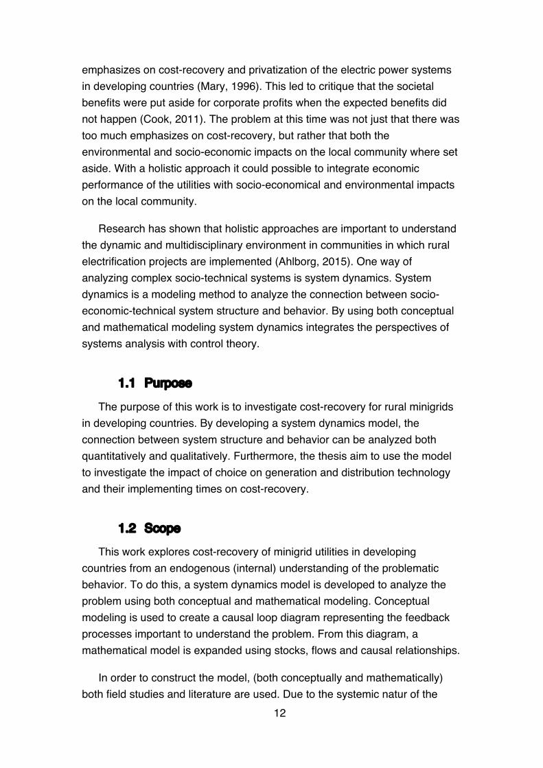
Figure 1 shows a graphical representation of a system. From Figure 1, it is seen that a system is compromised of a number of building blocks, called “Elements” connected with each other by “Relationships”. Based on these two concepts von Bertalanffy defined a system in 1968 “as a complex of interacting elements” (Bertalanffy, 1968). Each of the elements in a system has certain attributes that determine their properties. The system can also have one or more properties, the set of properties at any given moment in time is called the system state (Ackoff, 1971). The system state can be monitored via certain variables, named state variables. The state variables does not necessary reflect all the propoerties of the system.

Which elements and relationships that are included in the system is defined by the system boundary. As elements and relationships can be both physical and abstract, so can the boundary. Assuming a system has a

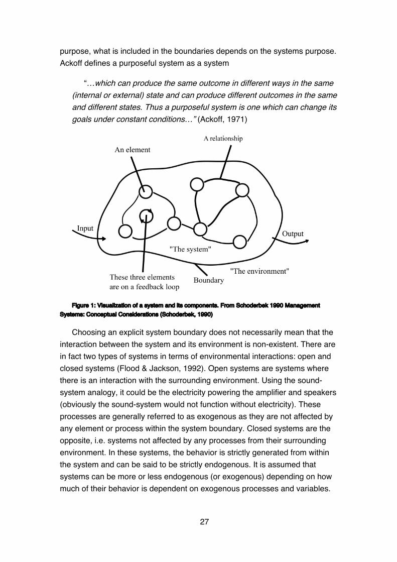
27

purpose, what is included in the boundaries depends on the systems purpose. Ackoff defines a purposeful system as a system

“…which can produce the same outcome in different ways in the same (internal or external) state and can produce different outcomes in the same and different states. Thus a purposeful system is one which can change its goals under constant conditions…” (Ackoff, 1971)

Figure 1: Visualization of a system and its components. From Schoderbek 1990 Management Systems: Conceptual Considerations (Schoderbek, 1990)

Choosing an explicit system boundary does not necessarily mean that the interaction between the system and its environment is non-existent. There are in fact two types of systems in terms of environmental interactions: open and closed systems (Flood & Jackson, 1992). Open systems are systems where there is an interaction with the surrounding environment. Using the sound-system analogy, it could be the electricity powering the amplifier and speakers (obviously the sound-system would not function without electricity). These processes are generally referred to as exogenous as they are not affected by any element or process within the system boundary. Closed systems are the opposite, i.e. systems not affected by any processes from their surrounding environment. In these systems, the behavior is strictly generated from within the system and can be said to be strictly endogenous. It is assumed that systems can be more or less endogenous (or exogenous) depending on how much of their behavior is dependent on exogenous processes and variables.

28

The endogenous behavior in systems is created when the element and interactions creates closed loops, called feedback loops (Sterman, 2000). Feedback loops can be of two types: reinforcing or balancing. A reinforcing feedback loop is a loop where an action produces a result which influence the same action, resulting in a growth or decline. A balancing loop on the other hand, is goal seeking, meaning it attempts to move the current state to some desired state (goal). Therefore, balancing loops are often referred to as goal seeking loops. However, goal seeking should not be mistaken for convergence, instead when combined with delays, balancing loops can cause over/under-shoot resulting in oscillating behavior.

A system can exhibit properties which are not found in any single part of the system (Flood & Jackson, 1992). These properties are created when parts of the system work together in synergy and are often called emergent properties (Flood & Jackson, 1992). Emergent properties can be seen as the opposite to the traditional reductionist and analytic view where systems can be broken down into smaller and smaller parts, each which can be studied individually.

Systems are commonly known to be hierarchic (Flood & Jackson, 1992). The concept of hierarchy is based on the assumption that systems are composed of interrelated subsystems (Herbert A. Simon, 1996). These subsystems are in turn hierarchic and consists of smaller subsystems, until an elementary subsystem is reached. One important property of hierarchy is that systems that are hierarchic evolves faster than non-hierarchic systems of a comparable size (Herbert A Simon, 1996). Two systems are said to be of comparable size if they both contain the same amount of elements. Simon describes that life might not exist if it wasn’t for hirerarchy since it is so improbable that matter would be arranged into living organisms if there where no stable subassemblies (Herbert A Simon, 1996).

3.2   System Dynamics

Our world is under accelerating change (Sterman, 2000). Technological development, economic growth, environmental degradation and globalization are just a few areas where change is happening fast, often so fast that we only react to the problems that occur too late. The driver behind change is the work to suppress the change that is perceived as being unfavorable and

29

promote change that we perceive as favorable. However, often the actions taken do not have the desired effects (J. Forrester, 1971).

Every time we face a situation when there is a need for us to make a decision, we try to our best capacity to anticipate the effects of different decisions and then chose the one decision that is most favorable to us. In order to do this we have a simplified perception of how our surrounding work. We use this simplified perception, or mental model, to anticipate the effects of our decisions. Our successfulness is then determined by how well our mental model correlates with the reality of the situation.

Phycologists have shown that our mental models can capture the behavior of only a few variables (Sterman, 1991). This might have been sufficient during our evolution but as our society has kept developing and become increasingly complex the number of occasions when our mental models fails have escalated. The reality might be much more complicated than what our mental models can cope with, and we even sometimes fool ourselves into taking the wrong decisions (Tversky & Kahneman, 1974).

System dynamics was developed as a tool to improve our understanding of complex societal systems, and more specifically to simulate effects of policies. It allows us to expand our understanding from our simple mental models to use the collective knowledge from actors in these systems. By formalizing and quantifying the underlying system structure in societal problems and how it is perceived by its actors, it is possible to use computers to simulate the effects of our actions, and what is often described as side effect, from our decision.

3.2.1  System Dynamics Theory Originating from control theory, system dynamics has one leg in

engineering where variables often are easy to identify and measure (“hard”). However, being an approach that is applied on societal problems, system dynamics struggles dealing with variables that are hard to identify and might not even be possible to measure (“soft”). The dilemma working with soft variables has been aknowleged in the system dynamics community from its beginning (J. W. Forrester, 1961). However, the difficulty in measuring and quantifying such variabels should not mean that they are excluded, or as Forrester formulated: “To omit such variables is equivalent to saying they have zero effect – probably the only value we know to be wrong!”

30

As in systems analysis and control theory, feedback is a basic concept in system dynamics. As described by Sterman (Sterman, 2000) a system dynamics model can be described as a set of feedback loops. It is the feedback loops and their relative strengths that generate the model behavior. Being a pragmatic modeling method, the feedback found in system dynamics models consists of causal links. Where causality is often interpreted as A casues B if a change of A results in a change of B, while nothing else is changed.

Stock and flow diagrams are one of two model representations in system dynamics. Unlike the causal loop diagrams (more on them later), stock and flow models are both conceptual and mathematical. Stock and flow models are built up by a set of feedback loops with each feedback loop consisting of at least one stock. The stock operates as a time delays in the system. In some feedback loops the time delays will be long and in some short and this differences in time delays creates the dynamics in the model. Often refered to as “change in loop dominance”.

Mathematically, a stock is equivalent to the integral of the flows connected with it. Or analogously, the flows are equivalent to the derivate of the associated stock. A simple example for a population with a fixed birth and death rate is shown in figure 2. The stock and flow structure shown in figure 2 can also be described mathematically as the differential equation 1.

Figure 2: Simple stock and flow model with one inflow and one outflow.

𝑃𝑜𝑝𝑢𝑙𝑎𝑡𝑖𝑜𝑛   = 𝐵𝑖𝑟𝑡ℎ  𝑅𝑎𝑡𝑒 − 𝐷𝑒𝑎𝑡ℎ  𝑅𝑎𝑡𝑒 ∙ 𝑑𝑡                                          ( 1 )

A closed feedback loop involving one stock and one flow is mathematically formulated as a differential equation, and since a stock and flow model consists of a set of connected feedback loops they are the equivalent of a set of coupled differential equations. Thereby they operate under the same assumptions and can use the same tools as in partial differential mathematics.

PopulationBirth Rate Death Rate

31

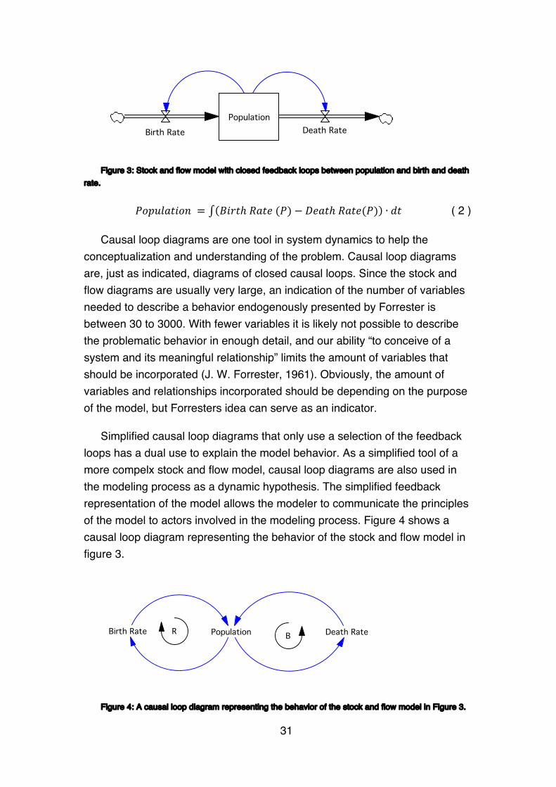
Figure 3: Stock and flow model with closed feedback loops between population and birth and death rate.

𝑃𝑜𝑝𝑢𝑙𝑎𝑡𝑖𝑜𝑛   = 𝐵𝑖𝑟𝑡ℎ  𝑅𝑎𝑡𝑒  (𝑃) − 𝐷𝑒𝑎𝑡ℎ  𝑅𝑎𝑡𝑒(𝑃) ∙ 𝑑𝑡                                        ( 2 )

Causal loop diagrams are one tool in system dynamics to help the conceptualization and understanding of the problem. Causal loop diagrams are, just as indicated, diagrams of closed causal loops. Since the stock and flow diagrams are usually very large, an indication of the number of variables needed to describe a behavior endogenously presented by Forrester is between 30 to 3000. With fewer variables it is likely not possible to describe the problematic behavior in enough detail, and our ability “to conceive of a system and its meaningful relationship” limits the amount of variables that should be incorporated (J. W. Forrester, 1961). Obviously, the amount of variables and relationships incorporated should be depending on the purpose of the model, but Forresters idea can serve as an indicator.

Simplified causal loop diagrams that only use a selection of the feedback loops has a dual use to explain the model behavior. As a simplified tool of a more compelx stock and flow model, causal loop diagrams are also used in the modeling process as a dynamic hypothesis. The simplified feedback representation of the model allows the modeler to communicate the principles of the model to actors involved in the modeling process. Figure 4 shows a causal loop diagram representing the behavior of the stock and flow model in figure 3.

Figure 4: A causal loop diagram representing the behavior of the stock and flow model in Figure 3.

PopulationBirth Rate Death Rate

Population Death RateBirth Rate BR

32

As a first step in system dynamics modeling put forward by Sterman is to create a dynamics hypothesis. A dynamic hypothesis is often visualized as a causal loop diagram and describes the variables and feedback loops the modeler believes are important for the problem. As the causal loop diagram contains feedback loops the description of the system is dynamic, hence dynamic hypothesis. The dynamic hypothesis works as foundation for the modeler both before and during data collection.

If system dynamics would have to be described with only one concept, it would likely be an endogenous understanding of the problem. Endogenous comes from the two words endo- meaning “within” and genous meaning “producing”. In terms of system dynamics models, this means that the models generate their behavior from the system structure, not from external influences. This is fundamentally different from many other modeling methods, where the user decides how a process (such as economic growth) is supposed to behave during the modeling period. A typical example are long term climate models that use a preset (exogenous) economic growth, thereby assuming that there is no relationship between the climate and economy.

System dynamics has been described as a bridge between the structure of and behavior in complex dynamic systems, since very simple structures have been found to generate very complex behavior (Davidsen, 1992). Structure is here understood to be the momentaneus relationships between parameters and the behavior to be the model state. As a stock and flow model is run there is a feedback between structure and behavior. The structure influence the state of the model, which influence the model structure. This is often reffered to as the structure-behavior feedback loop.

3.2.2  System Dynamics, Electric Systems Modellng and Development

System Dynamics has been used as a planning tool in the western electric power industry for decades (Ford, 1997; Teufel, Miller, Genoese, & Fichtner, 2013). Models have been used in a wide range of applications ranging from power plant construction times to energy system composition and transformation (Larsen & Bunn, 1999; H. Qudrat-Ullah & Davidsen, 2001; Teufel et al., 2013). Teufel et al. (2013) did a review of system dynamics based electricity models and found three trends: combination of methods, use of stochastic variables and increased level of detail. They also conclude that with the ability of system dynamics to incorporate qualitative aspects makes it

33

an appropriate method to be used in electric markets. The early System Dynamics models where almost exclusively constructed for countries or regions where the electricity access was very high and where only a small share or no people lacked access to electricity. This assumes that the electric infrastructure has reached a technological and institutional maturity not found in developing countries.

One of the first to develop a System Dynamics models specifically for the electric infrastructure in a developing country was Katherine Steel (2008). Her model analyzed the Kenyan electric power sector and the dynamics between grid and off-grid. Steel concludes that in Kenya the competition between grid and off-grid options is hurting the quality of electricity supply from the grid causing a downward reinforcing feedback loop of power quality. In some scenarios the downward spiral damaged the grid availability and reliability to the extent that off-grid electricity became the dominant supply of electricity. The model is based on consumer choice, where consumers can either connect to the grid, to an off-grid supply or change from one to the other. This assumes that there is a choice to be made by the users. However, since a large majority of the current population is living far from the grid receiving a grid connection in the foreseeable future is not likely and therefore no choice between grid and off-grid supply exist.

Steel’s model was followed by the work of Rhonda Jordan who analyzed long-term effects of capacity planning in developing countries, focusing on Tanzania and using System Dynamics and Linear Programming (Jordan, 2013). The purpose of the modeling was to find the optimal investments strategies in the electric power system based on endogenous behavior. Jordan concluded that it is important to incorporate endogenous electricity demand when either a large part of the population lacks electricity access or when adding new capacity bring improvements in reliability.

In rural electrification System Dynamics have been used to a lesser extent. However, there are more cases of System Dynamics models used in rural energy systems but these models have addressed the energy system and missed the technical representation of electricity (Mashayekhi, Mohammadi, Mirassadollahi, & Kamranianfar, 2010; Zhang, 2012). A few attempts have recently been made to either address specific technologies in rural electrification or addressing rural electrification on an abstract level (Fernando & Isaac, 2014) and therefore missing technology related dynamics and characteristics.

34

In the technologically oriented track of rural electrification research, modeling is relatively common. However, the models used in rural electrification have mostly modeled the operation and construction of technical systems, and often as optimization models trying to find the optimum choice of energy mixes or technology choice (Kanase-Patil, Saini, & Sharma, 2010; Nfah et al., 2008; Palma-Behnke et al., 2013). As technical models, they are limited to “hard”-variables and exclude variables seen as “soft” and difficult to quantify (Checkland, 2000; Jackson, 1985; Sterman, 2002). This has made the models very good at explaining the technical performance but lacks an integrated connection with rural economics and market growth theory, business administration and electricity usage. Hence they have been unable to endogenously describe the dynamics of cost-recovery.

35

4   Modeling as a Method

“I have not failed. I’ve just found 10 000 ways that won’t work.”

- Thomas A. Edison

What is a model? Why do we spend so much time building them? And what is their purpose? Modeling has penetrated almost all scientific disciplines, from political science, linguistics, logic, theoretical physics to engineering. A search in the sciencedirect database, representing 2500 journals with 13 million published papers, shows that almost half of those papers (5.5 million) contains the word “model” or “modelling”.

Even though the concept of models is much wider than to only include computer models, the computer has likely played an important role for modeling in science and engineering. This has possibly affected the general idea of what a model is and has in some areas made it synonymous with a mathematical representation of a system. Since in system dynamics this is not necessarily the case, this thesis will try to give a broader explanation here starting from research in philosophy of science.

In their “Models in Science” Frigg & Hartmann (2006) describes six different answers to, What is a model?: physical objects, fictional objects, set-theoretic structures, descriptions, or equations. Frigg & Hartman also describes that neither of these answers are exclusive and a model can therefore be any combination of the above. It is understood that models can preform two different functions (Frigg & Hartmann, 2006). A model can be a representation of a selected part of the world, i.e. a “system”. In this case the models can either be models of phenomena or models of data. Another function of models is that they can represent of a theory by interpreting the laws and axioms of the theory. One example could be the axioms in Euclidian geometry. Any structure in which these axioms are true can then be said to be a model of Euclidian geometry.

This theoretical approach to modelling can be found in some areas, such as Model Theory in mathematics. However, a short glance at the amount of publications or the available research grants is enough to see that research in applied science is overrepresented today. Models can be a very powerful tool to argue for ones case. However, since neither the models themselves nor the

36

processes of constructing them do not necessarily have to be transparent there is a risk that they end up being black boxes. Taking an input and generate an output without clearly stating the assumptions.

The first question any researcher using models in their work should ask is therefore: is modelling a suitable method to answer my question? In engineering disciplines where the researcher has access to all the relevant information and is able to formulate the question as a technical problem, the choice to use modeling or not is potentially more straight forward than for problems found in social systems. Social systems appear to be influenced by irregularity and lack of information (Featherston & Doolan, 2012).

A pragmatic view to modelling social science problems is found in the system dynamics community. The system dynamics method started out from applying control engineering to social science problems, which likely has helped keeping it pragmatic in terms of cases in which it has been used. One of the basic principles in system dynamics is that one does not model systems, but problems (J. W. Forrester, 1961; Sterman, 2000). However, this assumes that the questions one wants to answer can be formulated as a specific problem (and in the case of system dynamics as a dynamic problem, more on this later). This is not always the case, and the misbelief that system dynamics can be applied to all kinds of problems have resulted in cases where the choice of using system dynamics has not been correct. Non-critical use of system dynamics has led the method to receive bad reputation in some research areas, for example economics (Hayden, 2006; Radzicki & Tauheed, 2009).

An in-depth review of the criticism of system dynamics was recently done by Featherston & Dolan (2012). This thesis will not go into detail of Featherston’s & Dolan’s paper but will discuss two of the points mentioned: complexity and mimicry. One of the critiques brought up by Featherston & Dolan is the fact that social systems are open and irregular. Open meaning that social systems are to a large extent influenced by their surroundings. Since system dynamics does not attempt to model external influences, therefore fails at. System dynamics is a method to explore a problem through its endogenous behavior. If the problems are driven by exogenous influences then applying a system dynamics approach will not be beneficial. Not all problems are well suited to be investigated using an endogenous approach, which has led to system dynamics models being used for the wrong ‘type’ of problems.

37

One area that often receives criticism is the inability for system dynamics models to mimic reality (Keys, 1990; Solow, 1972). Tools are now available to most of the system dynamics software to allow for the modeler to fit his/her model to historical data. As noted in Sterman (Sterman, 2002), many modelers focus unreasonably on statistical fit and miss the more important underlying assumptions and appropriateness. In the system dynamics community it is widely accepted that system dynamics model cannot perfectly describe reality (Featherston & Doolan, 2012) and that the goal with system dynamics models is to improve the understanding between system structure and behavior, not to mimic reality.

Social systems can appear irregular, full with individuals making choices based on their free will. However, a deeper analyze reveals that our behavior is largely driven by rules, obligations, regulations and limitations (Featherston & Doolan, 2012). I as an individual might have the choice of paying or not paying when using the public transportation. But the descion to pay or not will partly be based on the risk of getting caught. Therefore, if I see any inspectors I will most likely pay for the ticket (assuming I don’t want to pay the fine and be exposed to the public humiliation of getting caught without a ticket).

In rural communities where electrification is taking place, a large number of actors and processes influence the descions individuals as well as organizations take. Access to environmental resources, financial capital, education, health, technology and infrastructure all affect these decisions. At the same time, the decisions taken affect the ability to derive benefits from and access to services in the future.

Observing these systems, they can seem complex. To be able to understand the underlying cause of their behavior one needs to use a method that has the ability to organize and analyze them. As a tool system dynamics has the ability to identify the underlying system structure in complex systems and map the structure to an observed behavior. Furthermore, as a modeling tool it integrates both the use of “hard” and “soft” variables making it an appropriate choice in simulation of electric power markets (Teufel et al., 2013).

4.1   The System Dynamics Modeling Method

The model presented in this thesis has been developed by using a method similar to Stermans iterative modeling process (Sterman, 2000). The process

38

Sterman proposes consists of five steps 1) Problem Articulation 2) Formulation of Dynamic Hypothesis 3) Formulation of a Simulation Model 4) Testing 5) Policy Design and Evaluation. Stermans modeling method has strong links to organizational management and policy evaluation. Since this work is a work in progress and since the purpose of this thesis is not to make any policy recommendations, the method has been slightly modified to fit into the context of rural electrification. Primarly this means that step 5) (Policy Design and Evaluation) has been removed. Figure 8 shows a conceptual map of the used modeling process.

Figure 5: The iterative modling process proposed by Sterman but excluding the last step, "Policy Formulation and Evaluation".

As system dynamics modeling is a conceptual and mathemtical tool to map system structure with system behavior, the modeling process can be seen to consist of two parts: information gathering for identification of the system structure and information gathering for populating the model’s parameters.

During the case studies both quantitative and qualitative data where collected. The quantitative data was mostly used for populating parameters and the qualitative data was mostly used to map the system structure. The qualitative data was collected through the interviews in two case subjects in Tanzania, which is further described in chapter 5. The process of mapping qualitative data to a conceptual model is understood to be hard. The process implemented during the modeling process, and specifically during the interviews, used in this thesis draws from the work presented by Chapman & Chapam (1971) and Kahneman & Tversky (1977) relating to biases in research. Questions where therefore first asked openly without trying to guide

1. ProblemArticulation

2. DynamicHypothesis

3. Simulation

4. Testing

39

the subject. Afterwards the subject where asked to verify or deny challanges identified previously.

The data for populating paramters where collected both through the case studies and via literature and reports. This means that parameter values had different origins and therefore different contexts. In cases where the parameter values where considered obviously inaccurate for a general context they where changed accordingly. This could be specific technology characteristics or specific electric equipment used. In a few cases no data where available and where therefore estimated. In these cases estimation was done taking into account model stability

With one year between the two case studies, when the field data where collected, it allowed for two iterations of the process described in figure 8. Furthermore, the data collected during the case visits where complemented with literature studies and discussions with advisors. The discussions and literature studies allowed for smaller iterations in the modeling process. The model iteration process is not finished and the model presented in this work is therefore still under development.

40

41

5   Data Collection

“No one will need more than 637 kB of memory...”

- Bill Gates2

Two visits where done to Tanzania for data collection. The two case studies subjects chosen where two villages in the south-western highlands. The villages where chosen to complement each other in terms of operation management. They are both comparable in size of 100 kW active generation capacity (village B also has an excess 100 kW installed but which wasn’t online at the time of visit due to low demand). They are both situated in the same region of Tanzania and therefore share similar environmental and regional conditions.

Village A and B where also chosen due to the their complementary electricity measurement systems. In village A, no system existed but the accessability to equipment was good and therefore high resolution measurements could be done. Village B on the other hand had a lower accessability to make high resolution measurements but instead had an automatic electricity surveillance system, where each users electricity usage was acquired on a monthly basis.

The different data types meant that the high resolution measurments from village A could be used for estimating the relation between power balance and energy balance. The lower resolution measured data from village B could be used for electricity usage growth rates and total electricity consumption on monthly time scales. During the case studies qualitative data on minigrid operation was also collected through interviews. The qualitative data was primarily used for identifying factors and interactions for the model construction.

5.1   Case study: Village A

Case study A was done in a village located in the southwestern highlands in Tanzania. Electricity is supplied to the village residents through a minigrid

2 Who actually said the qoute has been controversial, and some believe it

should rather be attributed to an employee at IBM.

42

operated by a local power utility. The utility has 264 customers, including a hospital, a small college, five mills and three workshops. To handle the relative large share of larger loads, the utility has put in place a running scheme, aiming at controlling when these loads are run. The grid is supplied with electricity from a nearby hydropower plant. The hydropower plant is of propeller type with a 120 kW generator and a small reservoir. The minigrid cover an area of approximately 2500 ha and its customers are supplied through an 11 kV transmission system and a 400V distribution system.

The power system is maintained and operated by a church with financial aid from international donors. One local engineer and one technician are responsible for the maintenance and operation together with help from a small administrative workforce. Income is generated using a flat tariff payment scheme dividing the customers into groups based on their estimated load. The tariff ranges from 5 000 to 35 000 Tanzania shillings (TZS), equal to about 3 to 20 USD/month using exchange rates from November 2014.

5.1.1  Measurements Assuming that most of an electric utility’s income is generated from

electricity sold and that utilization factor is important for cost-recovery, it is necessary to have high resolution data on electricity usage. From the literature it was found that there is much qualitative data on electricity usage but a lack of measured data for minigrids in developing countries (Blum et al., 2013; Cross & Gaunt, 2003). The data on electricity usage available in the literature is often collected through interviews or assumptions regarding which appliances exist and when they are run.

Interview based electricity usage methods are good in the sense that they require little or no expertise or equipment, making them very accessible, and that they have the ability to collect data on electric appliances and their usage. However, since users do not know exactly when they turn their appliances on and off and since users have different types of appliances, interview based electricity usage assessment lack accuracy and resolution. In order to have access to more detailed information on electricity usage, high resolution measurements on electricity usage was conducted.

Measurements was done at five users: one household, one rural hospital, one mill, one workshop and for the complete minigrid. The measurements where done using an Amprobe TRMS-16 Pro current clamp on meter. The device measures current through a conductor and stores three current values

43

each minute: low, average and high. Each measurement was done for three and a half days. Three measurements are shown in figure 6 to 8 below for the minigrid, household and for two milling machines and the workshop.

Figure 6: Measured daily load profile for village A. The Figure shows one black out at 10 and a planned shutdown for maintanence at 17. The load is measured in ampere and assumed to occur at nominal voltage (230 V). The hydropower plant is rated for 120 kW (180 A at nominal line-line voltage, 400 V).

Figure 7: Measured daily load profile for one household in village A. The load was measured in ampere and is assumed to occur at nominal line-neutral voltage (230 V).

44

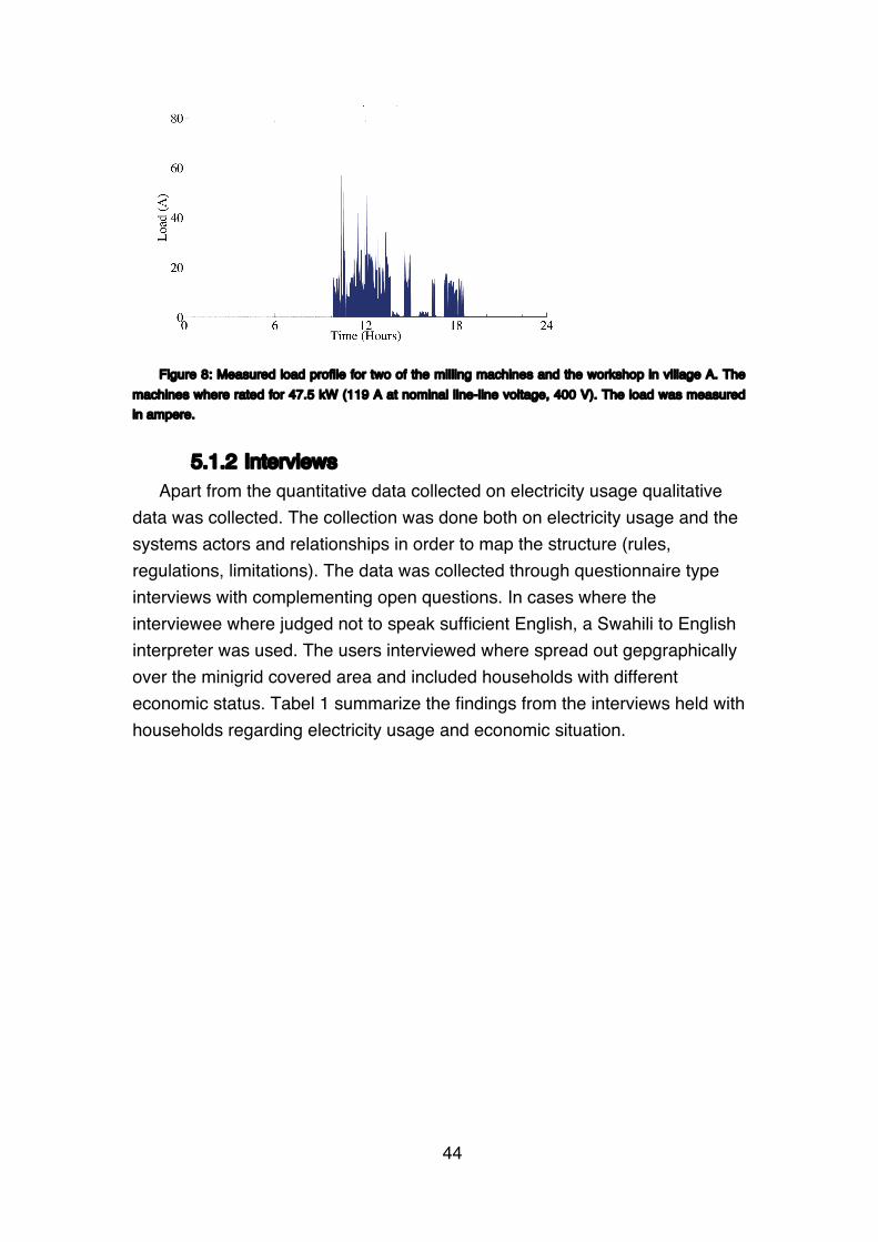
Figure 8: Measured load profile for two of the milling machines and the workshop in village A. The machines where rated for 47.5 kW (119 A at nominal line-line voltage, 400 V). The load was measured in ampere.

5.1.2  Interviews Apart from the quantitative data collected on electricity usage qualitative

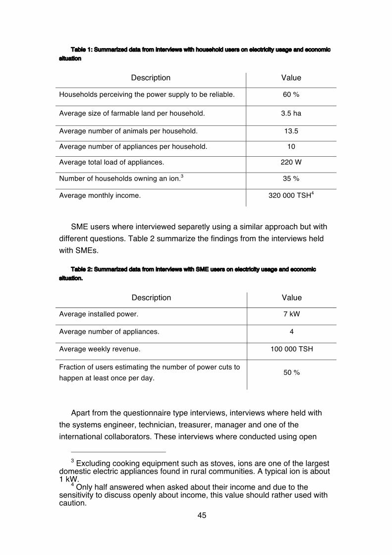
data was collected. The collection was done both on electricity usage and the systems actors and relationships in order to map the structure (rules, regulations, limitations). The data was collected through questionnaire type interviews with complementing open questions. In cases where the interviewee where judged not to speak sufficient English, a Swahili to English interpreter was used. The users interviewed where spread out gepgraphically over the minigrid covered area and included households with different economic status. Tabel 1 summarize the findings from the interviews held with households regarding electricity usage and economic situation.

45

Table 1: Summarized data from interviews with household users on electricity usage and economic situation

Description Value

Households perceiving the power supply to be reliable. 60 %

Average size of farmable land per household. 3.5 ha

Average number of animals per household. 13.5

Average number of appliances per household. 10

Average total load of appliances. 220 W

Number of households owning an ion.3 35 %

Average monthly income. 320 000 TSH4

SME users where interviewed separetly using a similar approach but with different questions. Table 2 summarize the findings from the interviews held with SMEs.

Table 2: Summarized data from interviews with SME users on electricity usage and economic situation.

Description Value

Average installed power. 7 kW

Average number of appliances. 4

Average weekly revenue. 100 000 TSH

Fraction of users estimating the number of power cuts to happen at least once per day.

50 %

Apart from the questionnaire type interviews, interviews where held with the systems engineer, technician, treasurer, manager and one of the international collaborators. These interviews where conducted using open

3 Excluding cooking equipment such as stoves, ions are one of the largest

domestic electric appliances found in rural communities. A typical ion is about 1 kW.

4 Only half answered when asked about their income and due to the sensitivity to discuss openly about income, this value should rather used with caution.

46

questions with the prupose for the respective subject to explain how he/she perceived the system to work. Interview subjects where chosen if they where deemed important actors in rural electrification from literature, or if they had been recommended in other interviews. Both actors working on site at minigrid projects, and actors working for governmental institutions in larger urban areas where interviewed.

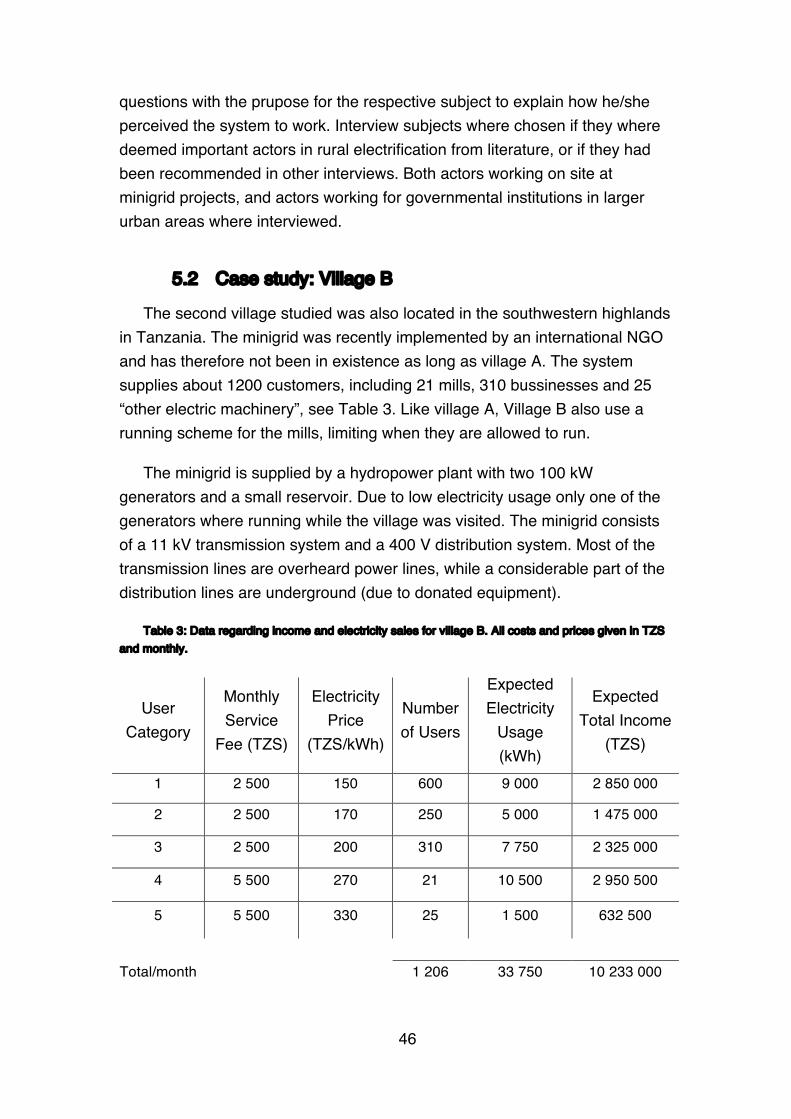
5.2   Case study: Village B

The second village studied was also located in the southwestern highlands in Tanzania. The minigrid was recently implemented by an international NGO and has therefore not been in existence as long as village A. The system supplies about 1200 customers, including 21 mills, 310 bussinesses and 25 “other electric machinery”, see Table 3. Like village A, Village B also use a running scheme for the mills, limiting when they are allowed to run.

The minigrid is supplied by a hydropower plant with two 100 kW generators and a small reservoir. Due to low electricity usage only one of the generators where running while the village was visited. The minigrid consists of a 11 kV transmission system and a 400 V distribution system. Most of the transmission lines are overheard power lines, while a considerable part of the distribution lines are underground (due to donated equipment).

Table 3: Data regarding income and electricity sales for village B. All costs and prices given in TZS and monthly.

User Category

Monthly Service

Fee (TZS)

Electricity Price

(TZS/kWh)

Number of Users

Expected Electricity

Usage (kWh)

Expected Total Income

(TZS)

1 2 500 150 600 9 000 2 850 000

2 2 500 170 250 5 000 1 475 000

3 2 500 200 310 7 750 2 325 000

4 5 500 270 21 10 500 2 950 500

5 5 500 330 25 1 500 632 500

Total/month 1 206 33 750 10 233 000

47

User category reflects different types of users with different electricity price. Category 1 are households with 1-7 electric appliances. Category 2 are households with 8 or more appliances. Category 3 are business, 4 are milling machines and 5 are other types of electric machines.

The income is generated by using a pre-paid system with digital meters and fixed monthly fees. The users can buy credits using common cellphone based payment services. Both the kWh price and the monthly varies for different users, with high demanding users paying more.

5.2.1  Interviews As in village A interviews in village B where done to map the structure of

the system in which actors and relationships took place. Interviews consisted of open questions and used a Swahili to English interpreter. On the utility side, technicians, the manager and treasurer where interviewed. Even though not part of the utility, the engineer responsible for the construction of the system was also interviewed.

The main purpose of the interviews done where for mapping the structure of the system dynamics model, therefore no interviews where done on electricity usage or appliance identification. Furthermore, other studies have identified different appliances and estimated electricity usage (Blum et al., 2013; Manning et al., 2015) but much less on the operation of rural utility’s.

48

49

6   Model Validation

“Reality is merely an illusion, albeit a very persistent one.”

- Albert Einstein

One of the major challenges for system dynamics models and modelers alike has been to become broadly acknowledged as a method in the scientific community. This has partly been influenced by the lack of widely accepted (outside the system dynamics community) standard validation methods. However, for the indulged there is a large amount of literature on the subject of validation methods and confidence building, both theoretical (Barlas, 1989, 1996; Senge, 1980) and case specific (Hassan Qudrat-Ullah & Seong, 2010).

The controversy of model validation is not specific for system dynamics but for all modelers alike. As discussed by Sterman (2000) one issue of validation is that many modelers consider a model validated when it is verified, i.e. when it is established as a truth. Assuming that a model can be “true” is in itself a contradiction since all models (regardless of they consist of equations, conceptual or literate) are simplification of the phenomena the researcher study. If a model cannot be said to be “true”, then validation in the sence of establishing truth cannot be made. This has been recognized by the system dynamics community since its early days, but has been controversial in other fields (Sterman, 2000).

In the system dynamics community, validity is instead closely linked with the concept of confidence (Senge, 1980). Instead of a process to establish “truthfulness”, validation is seen as a process of confidence building (Sterman, 2000). Confidence can be improved or detoriated using structured tests. The foundation of the concept of usefulness is that every model is made for a specific purpose and that the usefulness of a model is understood as how well the model fulfills its purpose (Barlas, 1996). Since the purpose of a model is decided by the modeler, and if the usefulness of a model relates to how well a model fullfil its purpose, then the model validation cannot be made completely objective (Barlas, 1996; Sterman, 2000).

A common validation test in the natural sciences and especially in engineering, is data fitting. The validity of a model is based on how well the model generates a certain output given a specific input. Using this anaology

50

the model is a black box, transforming an input to an output. Sometimes the understanding of what is inside the black box and how it works is not necessary. For example, an engineer working on the electric system for breaklights do not need to know how the breaks works, just that if the break is pressed the breaklights should turn on.

However, in many cases what is inside the box matters as much as its output. Likeley all undergraduate engineering students have at some time been told by their mathematics or physics teachers that: “it is not the answer that matters, but how you get there”. Getting the correct result is not sufficient unless you can explain why. In building confidence in system dynamics models there has been a strong emphasis on the “why?”, not just “that”.

“..a model must generate the right output behavior for the right reason.” (Barlas, 1996)

Shifting the focus from “what the results are” to “why are they like this” should rather than reduce the confidence in a model, increase it. Some system dynamicists have therefore proposed that the validation methods employed in system dynamics are stricter than those in other areas of modeling (Barlas, 1996).

The validation approach used in this work is based on holistic and relativistic philosophy proposed by Barlas & Carpenter (1990). It is based on that model validation cannot be made entirely objective and that a model can only be validated to its purpose. As proposed by Barlas and Carpenter validation is developed into two orders: structure validation and behavior validation.

Structure validation is the process of validating the models structure. In system dynamics this is done in two ways: direct structure tests and structure oriented behavior tests. Direct structure tests is done by comparing the processes, factors and parameters with real knowledge (when available, which in specific cases might not be the case). At this stage, dimensional consistency is tested and direct extreme condition tests. All these tests are done without any actual simulation.

The structure oriented behavior tests are tests focused on building confidence in the model structure through behavior. Can the model behavior be predicted in some cases? Usually, the behavior can be predicted under extreme conditions, for example using an extremely low or extremely high

51

connection cost. Unlike the direct structure tests, the structure oriented behavior test are done running the model under certain conditions.

Behavior validation is unlike structure validation, strictly a process to analyze the output from the model. However, this is not synonymous with fitting the model output to data but rather a test of the general behavior of the model. Does it increase when it should? Are the delays reasonable? How does it behave during extreme conditions? This includes tests described by Sterman (1984) and Forrester & Senge (1980).

One tool for confidence building of system dynamics models is the usage of historical data and the role of data fitting. As discussed earlier, data fitting should not be done excessively since it can shift the focus from the underlying assumptions of a model. Models are simplification of our perceived reality, and being simplifications, many processes and variables are not included. Spending too much resources in data fitting might therefore actually reduce the usefulness of the model and thereby its validity. Due to the difficulty to obtain and lack of long-term data on rural electrification a full stiatistical validation process has not been made. Instead we have compared specific variables against collected data for single time points. Using field data answers to questions such as “What is a reasonable income giving a certain amount of users and electricity consumption?” have been done. Even though this process lacks the full quantitative strength that a more comprehensive data fitting would produce, it does improve the confidence in the model.

52

53

7   System Dynamics Model of Cost-Recovery

“There is no abstract art. You must always start with something. Afterwards you can remove all traces of reality.”

- Pablo Picasso (1968)

By using theory available in literature together with information from the case studies in Tanzania, a system dynamics model was developed around the problem of achieving cost-recovery. The model is presented below in three parts. First, an overview of the model boundaries is presented, while more detailed assumptions are explained as the model is presented. Second is a causal loop diagram shown with the most prevalent feedback loops to describe the problem. The causal loop diagram is divided into two figures, one focusing on the causal relationship between electricity usage and economic growth.

Finally, after the causal loop diagram, the stock and flow model is presented. The complete stock and flow model includes 25 stocks, 137 variables and 54 constants over six sectors. A list and description of the stocks and their initial values can be found in the Appendix. Due to the size of the full stock and flow model, a simplified version is presented in this thesis.

7.1   Model Boundaries

As explained previously, the core of system dynamics lies in the endogenous description of behavior. Therefore it is important to not only include variables and processes which impact the behavior, but more importantly to include sufficiently feedback loops to describe the problematic behavior while not including too many. Where the boundary lie is difficult, however by using the iterative modeling method as described in chapter 4, the boundary selection is reevaluated during model construction.

Due to the very long time frame of some of the benefits associated with electrification, they have been either excluded or assumed to be exogenous. One such example is impact on health. As found by The World Bank (2008) improved health is identified as one area of improvement from increased

54

electricity access. It is assumed that the effect on health (using average life expectancy as an indicator) are slow in comparision to other effects (such as productivity and education). The model therefore assumes average life span exogenous, constant and based on sub-Saharan average.

As discussed earlier, the causal relationship between electricity and economic growth is disputable and many theories exist. This work makes no attempts to make any contribution to research in the causality between energy and economy, but use the direct causal connection via improved productivity, and certain indirect relationships identified in for example Kirubi et al. (2009) and Mulder & Tembe (2008). The implementation used in the model assumes a proctected market which allows external demand and exports but preserve the financial flows within the community.

Since the model assumes the perspective of an electric utility, access to electricity has been implemented in economical terms for the utility. This means that from the utility perspective only those who have made a connection has access. However, access can be used in a broader context relating to the benefits of electricity rather than a physical connection (Ahlborg, 2012). This has implications in terms of socio-economic development and life quality in the immediate surrounding of a connection, which partly since system dynamics is an aggregated modeling method is not treated explicitly in the model.

7.2   Causal Loop Diagram

Using the iterative method presented in chapter 4, a causal loop diagram has been developed during the modeling process. The causal loop diagram has been separated into two separate figures (9 and 10) to simplify the explanation. Figure 9 is centered around cost-recovery while figure 10 is an expanded diagram of the loop R3, showing the causal loops responsible for economic growth in a closed system.

Reinforcing loops are designated R and balancing loops are designated B. It should be noted, that not all feedback loops in Figure 9 are shown. But rather those that have been identified as most important through the research.

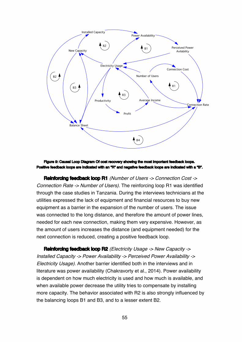
55

Figure 9: Causal Loop Diagram Of cost recovery showing the most important feedback loops. Positive feedback loops are indicated with an “R” and negative feedback loops are indicated with a “B”.

Reinforcing feedback loop R1 (Number of Users -> Connection Cost -> Connection Rate -> Number of Users). The reinforcing loop R1 was identified through the case studies in Tanzania. During the interviews technicians at the utilities expressed the lack of equipment and financial resources to buy new equipment as a barrier in the expansion of the number of users. The issue was connected to the long distance, and therefore the amount of power lines, needed for each new connection, making them very expensive. However, as the amount of users increases the distance (and equipment needed) for the next connection is reduced, creating a positive feedback loop.

Reinforcing feedback loop R2 (Electricity Usage -> New Capacity -> Installed Capacity -> Power Availability -> Perceived Power Availability -> Electricity Usage). Another barrier identified both in the interviews and in literature was power availability (Chakravorty et al., 2014). Power availability is dependent on how much electricity is used and how much is available, and when available power decrease the utility tries to compensate by installing more capacity. The behavior associated with R2 is also strongly influenced by the balancing loops B1 and B3, and to a lesser extent B2.

Balance Sheet

Number of Users

Electricity Usage

Average Income

New Capacity

Power Availability

Connection Cost

Profit

Productivity

Perceived PowerAvilability

Connection Rate

Installed Capacity

R1

B1R2

B2

B4

R3

B3

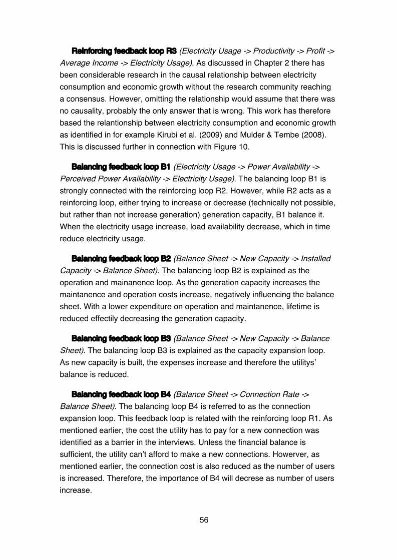
56

Reinforcing feedback loop R3 (Electricity Usage -> Productivity -> Profit -> Average Income -> Electricity Usage). As discussed in Chapter 2 there has been considerable research in the causal relationship between electricity consumption and economic growth without the research community reaching a consensus. However, omitting the relationship would assume that there was no causality, probably the only answer that is wrong. This work has therefore based the relantionship between electricity consumption and economic growth as identified in for example Kirubi et al. (2009) and Mulder & Tembe (2008). This is discussed further in connection with Figure 10.

Balancing feedback loop B1 (Electricity Usage -> Power Availability -> Perceived Power Availability -> Electricity Usage). The balancing loop B1 is strongly connected with the reinforcing loop R2. However, while R2 acts as a reinforcing loop, either trying to increase or decrease (technically not possible, but rather than not increase generation) generation capacity, B1 balance it. When the electricity usage increase, load availability decrease, which in time reduce electricity usage.

Balancing feedback loop B2 (Balance Sheet -> New Capacity -> Installed Capacity -> Balance Sheet). The balancing loop B2 is explained as the operation and mainanence loop. As the generation capacity increases the maintanence and operation costs increase, negatively influencing the balance sheet. With a lower expenditure on operation and maintanence, lifetime is reduced effectily decreasing the generation capacity.

Balancing feedback loop B3 (Balance Sheet -> New Capacity -> Balance Sheet). The balancing loop B3 is explained as the capacity expansion loop. As new capacity is built, the expenses increase and therefore the utilitys’ balance is reduced.

Balancing feedback loop B4 (Balance Sheet -> Connection Rate -> Balance Sheet). The balancing loop B4 is referred to as the connection expansion loop. This feedback loop is related with the reinforcing loop R1. As mentioned earlier, the cost the utility has to pay for a new connection was identified as a barrier in the interviews. Unless the financial balance is sufficient, the utility can’t afford to make a new connections. Howerver, as mentioned earlier, the connection cost is also reduced as the number of users is increased. Therefore, the importance of B4 will decrese as number of users increase.

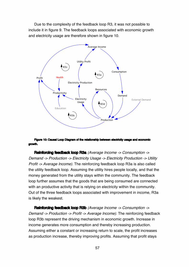
57

Due to the complexity of the feedback loop R3, it was not possible to include it in figure 9. The feedback loops associated with economic growth and electricity usage are therefore shown in figure 10.

Figure 10: Causal Loop Diagram of the relationship between electricity usage and economic growth.

Reinforcing feedback loop R3a (Average Income -> Consumption -> Demand -> Production -> Electricity Usage -> Electricity Production -> Utility Profit -> Average Income). The reinforcing feedback loop R3a is also called the utility feedback loop. Assuming the utility hires people locally, and that the money generated from the utility stays within the community. The feedback loop further assumes that the goods that are being consumed are connected with an productive activity that is relying on electricity within the community. Out of the three feedback loops associated with improvement in income, R3a is likely the weakest.

Reinforcing feedback loop R3b (Average Income -> Consumption -> Demand -> Production -> Profit -> Average Income). The reinforcing feedback loop R3b represent the driving mechanism in economic growth. Increase in income generates more consumption and thereby increasing production. Assuming either a constant or increasing return to scale, the profit increases as production increase, thereby improving profits. Assuming that profit stays

Demand

Profit

Consumption

Production

ElectricityUsage

Electricity Production

Average Income

Utility Profit

Productivity

Education

Health

External Demand

R3a

R3c

R3b

Resources

B3d

58

within the studied systems, the average income increase, further increasing consumption. It should be noted that this feedback loop is independent from electricity usage.

One important limitation of both R3a and R3b is that all processes are assummed to happen inside the community. If the profits are not gained by a community member, or spent on goods/services outside of the community, the feedback loop will be broken. These feedback loops are based on an closed economical system (but which allows an inflow of money as value is created).

Reinforcing feedback loop R3c (Average Income -> Consumption -> Demand -> Production -> Electricity Usage -> Productivity -> Profit -> Average Income). The feedback loop R3c, corresponds to impact on economic growth from electricity usage. As discussed earlier, the causality between electricity usage and economic growth is disputed and the assumption made in this work is that electricity usage improves the productivity of certain goods and services, which have been found in literature (Kirubi et al., 2009).

Reinforcing feedback loop B3d (Production -> Resources -> Production). Since all of the above mentioned feedback loops are positive and work in the same direction, they would drive economic growth indefinite. The balancing process assumed here is similar to what was used in the Limits to Growth model, World3, where the finite resources is a constrain on production. As production of goods/services increase, the localy available resource are reduced, limiting what, how much and for how long certain production systems can operate. One example is the available ecological resources where residences compete over the farmable land with larger scale commercial actors (Shete & Rutten, 2015).

59

7.3   Stock and Flow Model

From the causal loop diagram presented above, a stock and flow model was developed. Due to the number of variables and processes, the model where divided into six sectors: utility economy, connection of users, electricity usage, electric system expansion, local market and economy and population. Out of these six sectors, five are presented in this work. A simplified stock and flow model of population dynamics has been excluded due to its limited effect in the model.

Due to the size of the model, it is not presented in full detail in this thesis. However, the full stock and flow model, including equations, can be sent upon request. Instead a simplified stock and flow model is shown in Figures 5-9. Variables in the figures shown in grey and between “<>” are variables originating from another sector.

Figure 5 shows the simplified stock and flow model for the utilities balance sheet. The main income for the utility is the amount of electricity sold, which is dependent on the number of users and their respective electricity usage. As electricity usage vary largely depending on the user, both in terms of the amount of kWh consumed and when it is consumed, the model has two separate user groups: households and SMEs. Households tend to consume electricity during morning hours and in the evening while SMEs are more focused during the day (Hartvigsson et al., 2015). Since their effect on income for the utility is the same, figure 11 only contains one inflow while the full stock and flow model contains two inflows.

The utility’s expenses are to various degrees dependent on the size of the minigrid, both in terms of amount of users and generation capacity. The stock and flow diagram in figure 11 is mainly associated with feedback loops B2 and B3 in figure 9. However, since income is directly proportional to Electricity Usage, it is directly connected with the other feedback loops shown in Figure 2.

60

Figure 11: Simplified stock and flow model showing the income and expenses for the utility. Variables in grey marked with "< >" are variables originating from one of the other simplified stock and flow diagrams.

Income Statem

entUtility Incom

eM

aintenance Expenditure

Connection Cost

Capacity Expansion

Administration Cost

Number of Users

Electricity PriceCost for New

Capacity

<Installed Capacity>

<Planned Capacity>

<Connection Rate>

<Electricity Usage>

<Cost per Connection>

61

Figure 11 shows a simplified stock and flow diagram of the Income Statement. On the left side is the Income and on the right side the expenses. The generated income for a utility is assumed to be directly proportional to the amount of electricity sold, which is proportional to the amount of users and the electricity consumption of each user (together with electricity price). The utility has some ability to increase or decrease the electricity price based on their Income Statement.

The expenses are divided into four categories: Capacity Expansion, Maintanence and Operation, Connection Costs and Administration Costs. Capacity Expansion are expenses associated with constructing more generation capacity. These costs are not continuous but is a single value deducted from the Income Statement if the current capacity is not sufficient and the utility has the funds for constructing more capacity. Maintanence and Operations are connected with the generation capacity and affects the deterioration time of the equipment. Connection costs are the costs for connection of new users, which is dependent on the connection rate and the cost of connection. Both which are explained more in detailed in Figure 12. Lastly is admistrative costs. Administrative costs are assumed to be consisting of two parts: one is fixed for the system and one is dependent on the number of users. Administrative costs are assumed to include all costs associated with personal.

Therefore, one important purpose of the model is to describe the dynamics and feedbacks related to the growth in number of users and changes in electricity consumption. The simplified stock and flow diagram explaining the connection rate is shown in figure 12. The connection process is based on Eder et al. description the user growth in a minigrid as a diffusion process (Eder, Mutsaerts, & Sriwannawit, 2015; Rogers, 2010). Eder et al. used a multidisciplinary perspective to identify three dimensions that affect diffusion of electricity adoption: technology, economy and society. Amongst these dimensions Eder et al. identified key variables, such as reliability, connection cost, tariffs and perception of electricity.

62

Figure 12: Simplified stock and flow model showing the connection processes. Variables in grey marked with "< >" are variables originating from one of the other simplified stock and flow diagrams.

Non-UsersUsers

Connection Rate

Non-Users DesiredConnection Rate

Utility DesiredConnection Rate

Price per Connection

Risk

User Density

Technical Personel

Fixed cost perConnection

Cost per Connection

Population Growth

Equipment Cost

Fertility Rate

<Power Availability>

<Income Statem

ent>

<Income>

63

During the case studies in Tanzania, the local utility’s capacity to connect new users was identified as a barrier for growth in number of users. The utilities’ capacity can be limiting in terms of the amount of technicians able to perform connections and the utility’s available financial resources that are needed to buy equipment (power lines, poles, etc.). The connection rate is therefore divided into two separate processes: users desired connection rate and the utility’s desired connection rate.

The users desired connection rate is based on their income, the price of a connection and the perceived risk. Risk is assumed to consit of three parts: financial risk, technical risk (reliability) and social acceptance. Financial risk is implemented as the change in connection price. During the initialization the price is normalized and as connection price is deacreased the risk is also decreased. Reliability is connected to the perceived Power Avilability. If the Power Availability is poor the risk of a connection is increased. Furthermore, if the Power Availability is considered extremely poor, the direction of the connection rate is changed and people start disconnecting from the minigrid.

The utility’s desired adoption rate is assumed to be dependent on the cost per connection, the utility’s economic balance and the number of technical personnel. The cost per connection is assumed to be proportional to the distance to the closes point of connection, which in turn is dependent on the user density. The distance is assumed to decrease linearly with user density. Even if the utility has enough financial and technical resources, the utility is limited by the number of personnel with the knowledge to make new connections.

64

Figure 13: Simplified stock and flow diagram of the dynamics of electricity usage. Variables in grey marked with “<>” are variables originating from one of ther other simplified stock and flow diagrams.

Figure 13 shows a simplified stock and flow diagram for the dynamics of Electricity Usage. Electricity Usage is assumed to be directly influenced by four variables: Income, Power Availability, Electricity Price and Fraction of Income Spent on Electricity. It is further assumed that the Fraction of Income Spent on Electricity is dependent on installed load (i.e. how many and which type of appliances the user have).

The type of and number of appliances is dependent on “Installed Load”, and it is assumed that the type and amount of appliances is dependent on “Income”. Making “Income” an indirect factor influencing the “Fraction of Income Spent on Electricity”. The long term data collected from village B on monthly electricity usage was used as a reference for reasonable growth rates and user consumption.

The effect of Power Availabilty on Change in Electricity usage is assumed to be non-linear. As long as Power Avilabilty is 1 or less, there is no impact on Change in Electricity Usage. However, if Power Availabilty is slightly larger than 1, meaning that there is an overload in the electric system, Electricity Usage starts slowly to decrease. For high values (around 1.1-1.2, meaning the electric system is heavily overloaded) electricity usage and number of connections is rapidly decreased.

Electricity UsageChange in

Electricity Usage

<Power Availability>

Fraction of IncomeSpent on Electricty

<Installed Load><Income>

<Electricity Price>

65

Figure 14 shows a simplified stock and flow diagram for the capacity expansion. The capacity expansion loop consists of two stocks, Installed Capacity and Planned Capacity, and therefore two capacity flows, “Planning Process” and “Construction”. In terms of model behavior, there is no difference between “Planning Time” and “Construction Time” but only the total time from a descion to “power on”. However, from an policy point of view it is interesting to know if the delays are technology dependent or if they are based on bureaucratic procedures.

It is assumed that capacity expansion can only be done in discrete blocks, which are technology dependent. Furthermore, the utility is allowed to take a load of up to 70% of the capacity expansion cost if needed. This theoretical bank allows the utility to respond faster to a change in demand if its financial resources are limited. As the purpose is to investigate the endogenous behavior, the problematic behavior of reaching cost-recovery and not external factors, the interest rate on the loan is excluded.

Capacity size is exogenous and can be set by the user. Capacity also detoriate with time, and the deterioration time is dependent on the expenditure on “Operation and Maintanence”. If “Operation and Maintanence” is kept at the desired level, the deterioration is linear. If the utility cannot afford to pay operation and maintanence costs and therefore accelerate the deterioration time.

During the development of the power expansion sector, the measurement data from village A was used to estimate how much load a rated capacity can supply, also known as coincidence factor. Based on the measurements a constant coincidence factor of 0.5 is used in the model. Meaning, that a capacity of 200 kW can supply a installed load of 400 kW. This means that the power availability is 1 when the installed load is twice of the generation capacity. Normally the coincidence factor varies depending on local factors such as type, number and mix of customers, types of electrical appliances and time of the day.

66

Figure 14: Simplified stock and flow diagram of capacity expansion and load dynamics. Variables in grey marked with "< >" are variables originating from one of the other simplified stock and flow diagrams.

Planned CapacityInstalled Capacity

ConstructionDepreciation

Planning Process

Desired Capacity

Cost of Capacity

Construction Time

Planning Time

Depreciation Time

Installed Load

Power Availability

Change in Load

Capacity Size

<Number of Users>

<Income Statem

ent>

<Maintenance Expenditure>

<Income>

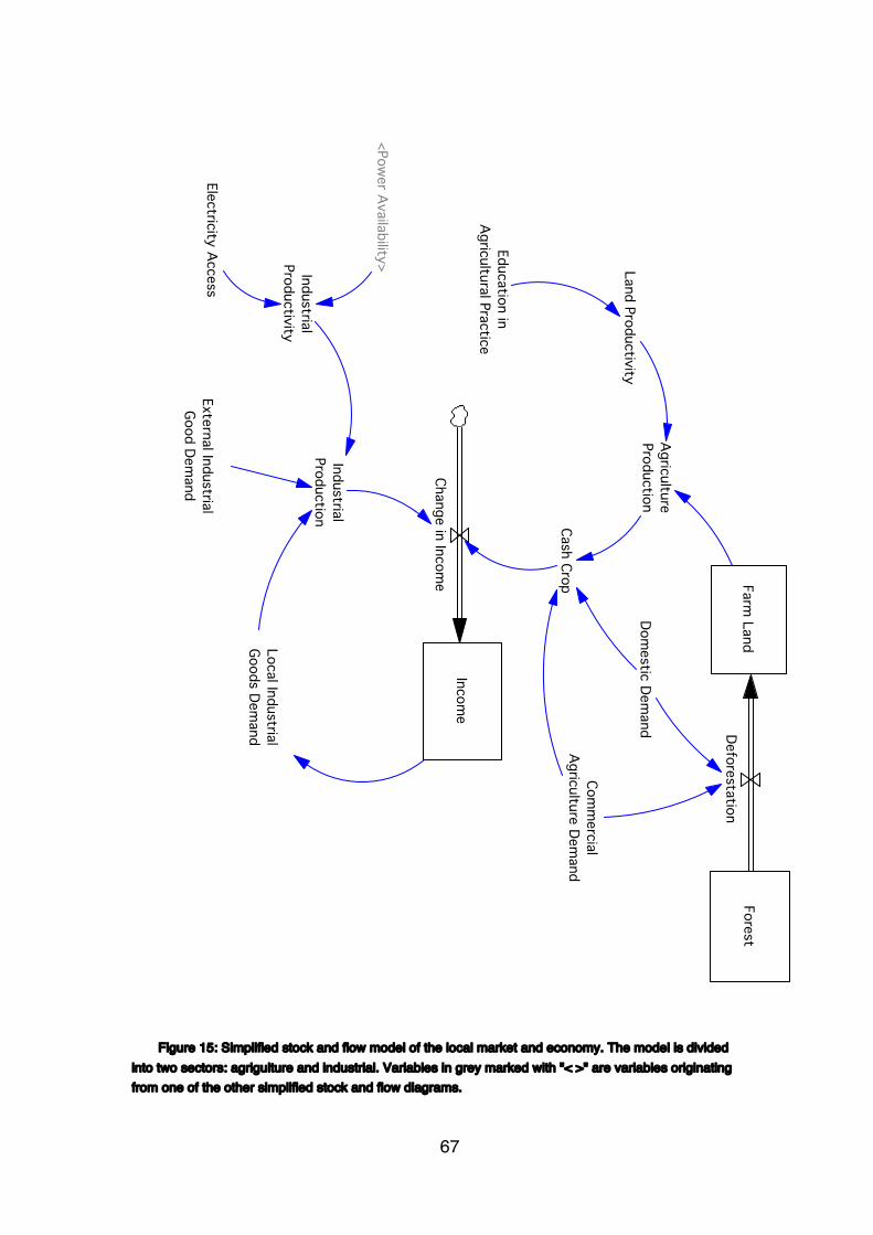
67

Figure 15: Simplified stock and flow model of the local market and economy. The model is divided into two sectors: agrigulture and industrial. Variables in grey marked with "< >" are variables originating from one of the other simplified stock and flow diagrams.

Income

Change in Income

Cash Crop

IndustrialProduction

Farm Land

Domestic Dem

and

Local IndustrialGoods Dem

and

External IndustrialGood Dem

and

Land Productivity

AgricultureProduction

Education inAgricultural Practice

IndustrialProductivity

Electricity Access

ForestDeforestation

Comm

ercialAgriculture Dem

and

<Power Availability>

68

As disposable income is one of the major variables affecting number of users and electricity usage, the change in disposable income will affect both long-term connection rates to the minigrid and changes in electricity consumption. According to Davis et al. (2010) the majority of income in rural sub-Saharan Africa is generated from agricultural production and a minority is coming from non-agricultural activities. Furthermore, Davis et al. found associations between the share of non-agricultural activities and income, with income rising as non-agricultural activities increased. As reported by Bardi et al. (2013) another difference between agricultural and non-agricultural activities is the ability for improvements when electricity is used. Non-agricultural activities can to a larger extent be improved than agricultural activities.

Assuming incomes either come from agriculture or industrial activities a two-sector market model is developed. Both the agricultural and industrial production is assumed to be driven by demand, assuming a demand-pull market. According to Coombs et al. (1987) demand-pull is limited to improvements in already existing production and do not include the formation of new producers. In the model this is implemented as the growth of SMEs is exogenous to the model.

Regarding income from agricultural production, there are two ways to increase the agricultural production per household, either through increase in farmed land or by increasing land productivity. When it comes to the land size the amount of farmable land is limited. Agriculture land competes with both industrial services (such as industrial timber production) and pressure on leaving forest areas untouched to keep biodiversity. Furthermore, individual farmers also compete about access to the most fertile land. The ability to increase a household’s land area is also connected with the household’s income and the price for obtaining more land. This can create a barrier for poor households to increase their production. The second approach to increase agricultural production is through improved land productivity. This is assumed to mainly be driven by education in agricultural practices (Chang & Zepeda, 2001). Other factors, such as access to technologies also affects productivity to some extent. It is here assumed that access is not a barrier, and if a farmer has the appropriate knowledge he/she can aquire the needed technology.

As mentioned above, local production is described as a demand-pull process and therefore excludes formation of new producers. Assuming that

69

access to other markets is important for economic growth, the model incorporates an external demand function. This external industrial demand is modeled exogenously and is similar to a push processes in terms that it can increase local production without increasing local demand.

70

71

8   Technology Evaluation and Cost-Recovery

“The formula ‘two and two makes five’ is not without its attractions.”

- Fyodor Dostoevsky (1864)

The fact that technology impacts the successfulness in rural electrification is clear, but how and to what extent is not as apparent. As mentioned earlier in the thesis, technology is often seen as a exogenous variable supplying electricity for a given cost (see Kaundinya et al. (2009) for a review of technical rural electrification studies). However, energy sources have many more characteristics, which are depending on the context can play an equal important role as cost. Some of these characteristics can play an especially important role in minigrids in developing countries where changes can happen very quickly. As found by a report from The World Bank (2007), one of those characteristics is the time from decision to “power on” for electricity generation. “Power on” is here referred to as the moment when users get access to electricity provided by new generation capacity.

There are obviously multiple variables affecting the time between decision and “power on”. The underlying reason for the delay is not specified here but would be of interest when it comes to implementing policies. A few examples of underlying factors could be the demand for permits, access to technology and construction time. It is assumed that energy sources/facilities that provides more power will have a longer construction and planning time. For example, the planning and construction time for a 100 kW power plant is considerable longer than that of a 1 kW power plant.

One characteristic of distribution technology is its power limitations. Generally an electric power system that needs to distribute more power is more costly to construct. As was identified through the interviews with rural electrification consultants and minigrid operators, that the costs to make a new connection is sometimes a barrier for a utility to increase the number of users. The interviews and measurements also revealed that most users had a very low power consumption but still a higher power supplying connection. This was confirmed during the interviews with one of the foreign consultancy companies working in the Tanzanian electric power sector, stating that only a

72

few percent of surveyed users requests a 3-phase connection for operating larger machinery, such as electric motors.

8.1   Simulation Specific Data

Using variables for cost, planning and construction time, power plant size, connection cost and limitations on installed load, the model is used to investigate the behavior of minigrid utilities on technologic specific characteristics. In total six different cases are simulated, representing different characteristics of technology.

Below follows figures with result generated from six runs. The results are divided into two sections, first without any limits on electric loads (similar with that of a standard 3-phase system) and second with limits on SME electric loads for SMEs. Furthermore, when the SME load is limited the initial average installed load is also lower, compared without any limits. Each of these cases is then divided into three sub-cases with different sizes of rated capacity: 1 kW,10 kW and 100 kW. It is assumed that larger generation capacities has lower costs per kW.

All changes in variables represent characteristics that can be found amongst technologies used in rural electrification. The 1 kW case is similar to a solar PV system, 10 kW a small scale wind power system and the 100 kW a hydropower expansion (assuming in this case that the previous generation system is based on hydropower). The limitations on installed load per SME user, and thereby a reduced cost of connection are characteristics that are shared with a SWER5 system (Al-Mas, 2010). The above mentioned parameters are summarizied in table 4. CC mentioned in the table 4 is an abbrevation for Connection Cost. The initial values for the model’s stocks can be found in the Appendix.

5 SWER – Single Wire Earth Return is a distribution technology that only

uses one conductor, unlike the standard three-phase’s three conductors, making it cheaper but also limits the transferable capacity.

73

Table 4: Information on parameter values for simulations.

1 kW (PV) 10 kW (mini wind) 100 kW (hydro)

No-limit (3-phase) 2000 USD/kW6

(100 % cc) 1500 USD/kW7

(100 % cc) 500 USD/kW8

(100 % cc)

Limit (SWER) 2000 USD/kW

(60 % cc) 1500 USD/kW

(60 % cc) 500 USD/kW

(60 % cc)

The initial state of the model during the simulations is set to share charateristics with the two case study villages. It is assumed that the initial generation capacity can supply stable electricity 24 hours per day, 7 days a week. Due to the choice of representations of technologies in table 1, it is assumed that the initial generation capacity can be expanded relatively easy.

To present the simulations three stocks where chosen as indicators of the utility’s performance: economic balance, generation capacity and electricity usage. The simulations are shown as 3D figures with time on the x-axis, Construction and Planning Time on the y-axis and the corresponding indicator on the z-axis. The figures also show a semitransparent red plane on the Construction and Planning Time axis and aims to give an indicator of Constrution and Planning Times for the three different generation capacity sizes. The red plane is situated at 25 weeks for 1 kW, 52 weeks for 10 kW and 100 weeks for 100 kW generation capacities. Due to different results in the simulations and to clearly show the behavior the z-axis is scaled according to each simulation.

8.2   Small Rated Capacity – Without SME Load Limit

Figure 16 to 18 shows the results for the simulations without any load limit and with the 1 kW rated generation capacity. Figure 16 shows the balance sheet (in USD) of the utility. Figure 17 shows the installed generation

6 Price estimate taken from (IRENA, 2015) 7 Price estimate taken from (Ltd, 2006) 8 Price estimate taken from (IRENA, 2012)

74

capacity of the system on the z-axis ranging from 160 – 280 kW and figure 18 shows the total electricity usage (in kWh).

From the figures it is seen that as the construction and planning time increase the electricity usage and capacity decrease. As the construction and planning time increase it becomes difficult for the utility to keep supplying power to follow the demand. This reduces the power availability, which negatively influence electricity usage. As the construction and planning time increase, the point at which newly acquired capacity is turned online comes later. This is seen as the diagonal wave pattern in all figures (but more clearly in figure 16 and figure 17).

The fast reduction in Balance sheet seen in figure 16 during the first weeks is a direct result from increase in connections. As the utility is initialized with 10 000 USD, it has the economic capacity to connect more users. Since there is a demand from the non-users and due to the high cost per connection initially (as mentioned earlier, connection cost is proportional do the distance to the closes connection cost).

The seemingly high and fast variations in the balance sheet for short construction and planning times is the result from the short time and the small rated capacity (a small size means lower costs and the utility therefore needs shorter time to reach enough income in order to expand). The utility therefore can follow the electricity demand as it increase.

75

Figure 16: Shows the impact from different ”Construction and Planning Times” on Utility Balance during the modeled time frame. The semitransparent red square marks 25 weeks of ”Construction and Planning Time”.

Figure 17: Shows the Generation Capacity of the minigrid. Even during normal operation, the capacity is deteriorating due to wear and tear from operation. The semitransparent red square marks 25 weeks of ”Construction and Planning Time”.

76

Figure 18: Shows the total “Electricity Usage” for the minigrid system. The semitransparent red square marks 25 weeks of ”Construction and Planning Time”.

8.3   Medium Rated Capacity – Without SME Load Limit

Figure 19 to 21 shows the results for the simulations without any load limit and with the 10 kW rated generation capacity. Figure 19 shows the balance sheet (in USD) of the utility. Figure 20 shows the installed generation capacity of the system on the z-axis ranging from 60 – 200 kW and figure 21 shows the total electricity usage (in kWh).

Like in the previous case, during the first weeks, the utility use the initial captial to connect more users, resulting in an increase in electricity consumption and followed by a modest increase in income. As time progress, electricity usage per user increase due to market growth (income is increased leading to larger expenditures on electricity). Parallel to the increase in electricity usage, generation capacity is deterioting due to wear and tear. These two processes continue for approximately 300 weeks when electricity demand has caught up with generation capacity and therefore reduce power availability.

77

As the power availability is reduced the electricity usage is decreased, reducing the utility’s income but also increasing the power availability. However, as the utility’s income is not enough to expand the generation capacity, the electricity usage will keep reducing as the generation capacity is detoriating. This process continues until the utility’s income can’t cover basic operation and maintanence of the plant. Without any operation and maintanence the plant quickly deterioates (seen around week 900).

Figure 19: Shows the impact from different ”Construction and Planning Times” on Utility Balance during the modeled time frame. The semitransparent red square marks 52 weeks of ”Construction and Planning Time”.

78

Figure 20: Shows the Generation Capacity of the minigrid. Even during normal operation, the capacity is deteriorating due to wear and tear from operation. The semitransparent red square marks 52 weeks of ”Construction and Planning Time”.

Figure 21: Shows the total “Electricity Usage” for the minigrid system. The semitransparent red square marks 52 weeks of ”Construction and Planning Time”.

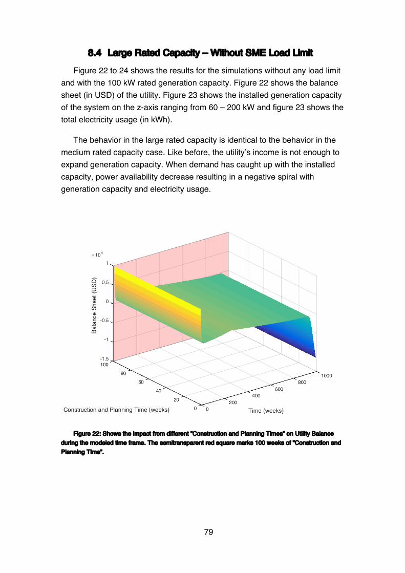
79

8.4   Large Rated Capacity – Without SME Load Limit

Figure 22 to 24 shows the results for the simulations without any load limit and with the 100 kW rated generation capacity. Figure 22 shows the balance sheet (in USD) of the utility. Figure 23 shows the installed generation capacity of the system on the z-axis ranging from 60 – 200 kW and figure 23 shows the total electricity usage (in kWh).

The behavior in the large rated capacity is identical to the behavior in the medium rated capacity case. Like before, the utility’s income is not enough to expand generation capacity. When demand has caught up with the installed capacity, power availability decrease resulting in a negative spiral with generation capacity and electricity usage.

Figure 22: Shows the impact from different ”Construction and Planning Times” on Utility Balance during the modeled time frame. The semitransparent red square marks 100 weeks of ”Construction and Planning Time”.

80

Figure 23: Shows the Generation Capacity of the minigrid. Even during normal operation, the capacity is deteriorating due to wear and tear from operation. The semitransparent red square marks 100 weeks of ”Construction and Planning Time”.

Figure 24: Shows the total “Electricity Usage” for the minigrid system. The semitransparent red square marks 100 weeks of ”Construction and Planning Time”.

81

8.5   Small Rated Capacity – With SME Load Limit

Figure 25 to 27 shows the results for the simulations with load limit and with the 1 kW rated generation capacity. Figure 25 shows the balance sheet (in USD) of the utility. Figure 26 shows the rated generation capacity of the system on the z-axis ranging from 100 – 400 kW and figure 27 shows the total electricity usage (in kWh).

Like in the analogous case but without a load limit, the utility achieve to reach cost-recovery and manage the system in a stable way. However, the utlity does not only manage to reach cost-recovery but is generating considerable income, higher installed capacity and more electricity usage compared to the case without load limit.

One economical challenge for minigrid utilities is the long payback time for each connection. I.e. the time it takes before the customer has generated enough income for the utility to pay for the connection cost. When the connection cost is reduced, the payback time is proportionally reduced. With the reduced connection cost the utility can afford almost twice the amount of connections (the connection cost is proportional to distance which is assumed to be logarithmically decreasing with number of connections). The increase in number of users have a larger impact on total electricity usage than the increase in per user electricity usage.

The diagonal “valleys” seen in figure 25 are an effect of investments in new generation capacity. The width of a valley (for a fixed construction and planning time) is constant and roughly equal to the consutrion and planning time. It should be noted, that even though it might seem like the utility has more financial captial according to figure 25 the utility has invested in less generation capacity.

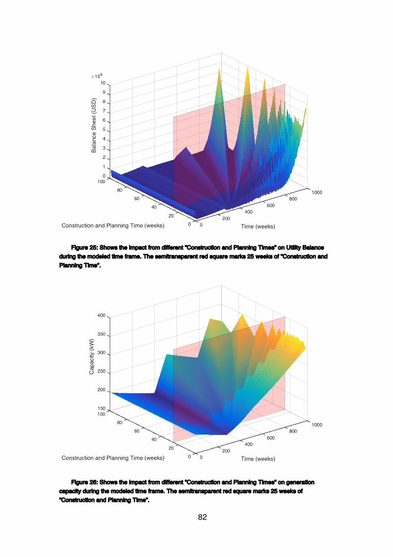
82

Figure 25: Shows the impact from different ”Construction and Planning Times” on Utility Balance during the modeled time frame. The semitransparent red square marks 25 weeks of ”Construction and Planning Time”.

Figure 26: Shows the impact from different ”Construction and Planning Times” on generation capacity during the modeled time frame. The semitransparent red square marks 25 weeks of ”Construction and Planning Time”.

83

Figure 27: Shows the impact from different ”Construction and Planning Times” on electricity usage during the modeled time frame. The semitransparent red square marks 25 weeks of ”Construction and Planning Time”.

8.6   Medium Rated Capacity – With SME Load Limit

Figure 28 to 30 shows the results for the simulations with load limit and with the 10 kW rated generation capacity. Figure 28 shows the balance sheet (in USD) of the utility. Figure 29 shows the rated generation capacity of the system on the z-axis ranging from 100 – 500 kW and figure 30 shows the total electricity usage (in kWh).

Unlike in the analogous case without load limit, the utility manages to reach cost-recovery and generate a profit. The explanation is similar to what made the utility improve its economic balance in the small rated capacity case. With the reduced connection cost, the utility can increase the amount of users and thereby improve its income. The increased income is sufficient for the utility to expand the generation capacity as demand increase.

Furthermore, compared to the small rated capacity case with load limit, the generated profit is generally higher. However, the presented figures do not show capacity being built (but which have been paid for). In the small rated

84

capacity case, due to the delay in construction the utility pile up a capacity. Hence if the graphs would have taken into account this capacity, the difference in balance would be swapped.

Figure 28: Shows the impact from different ”Construction and Planning Times” on Utility Balance during the modeled time frame. The semitransparent red square marks 52 weeks of ”Construction and Planning Time”.

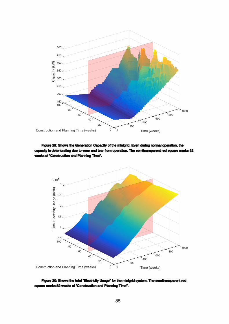
85

Figure 29: Shows the Generation Capacity of the minigrid. Even during normal operation, the capacity is deteriorating due to wear and tear from operation. The semitransparent red square marks 52 weeks of ”Construction and Planning Time”.

Figure 30: Shows the total “Electricity Usage” for the minigrid system. The semitransparent red square marks 52 weeks of ”Construction and Planning Time”.

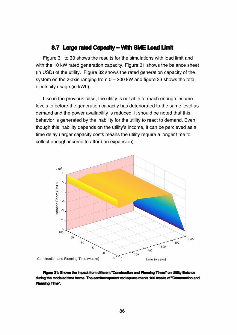
86

8.7   Large rated Capacity – With SME Load Limit

Figure 31 to 33 shows the results for the simulations with load limit and with the 10 kW rated generation capacity. Figure 31 shows the balance sheet (in USD) of the utility. Figure 32 shows the rated generation capacity of the system on the z-axis ranging from 0 – 200 kW and figure 33 shows the total electricity usage (in kWh).

Like in the previous case, the utility is not able to reach enough income levels to before the generation capacity has deteriorated to the same level as demand and the power availability is reduced. It should be noted that this behavior is generated by the inability for the utility to react to demand. Even though this inability depends on the utility’s income, it can be percieved as a time delay (larger capacity costs means the utility require a longer time to collect enough income to afford an expansion).

Figure 31: Shows the impact from different ”Construction and Planning Times” on Utility Balance during the modeled time frame. The semitransparent red square marks 100 weeks of ”Construction and Planning Time”.

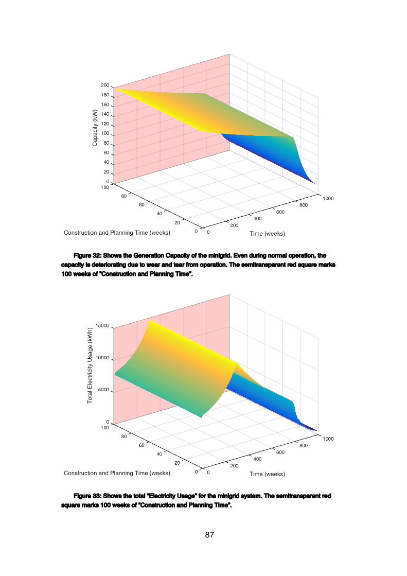
87

Figure 32: Shows the Generation Capacity of the minigrid. Even during normal operation, the capacity is deteriorating due to wear and tear from operation. The semitransparent red square marks 100 weeks of ”Construction and Planning Time”.

Figure 33: Shows the total “Electricity Usage” for the minigrid system. The semitransparent red square marks 100 weeks of ”Construction and Planning Time”.

88

89

8.8   Summary of Simulations

Table 5 below summarize the results depending on the load limitations and rated capacity size. The cases where the utility achieve cost-recovery are marked with an “x”, and the cases where the utility fails are marked with an “o”.

Table 5: Table showing a summary of results from simulations.

Small (1 kW)

Medium (10 kW)

Large (100 kW)

No-Limit x x o

Limit x o o

For the small rated capacity, the change of distribution technology from No-Limit to Limit changes the economic successfulness. Whithout any load limit, the utility can handle changes in demand, but does not make any larger profits. When the load limit is in place, the utility can afford more connects and thereby generates more income. The improved income leads to the increased profit.

In the medium rated capacity case, the replacement of distribution technology from No-Limit to Limit change the result from economic collapse to reaching cost-recovery and profit generation. With the load limit, the utility cannot afford to reach enough users and thereby not enough income to be able to invest in more generation capacity when the demand requires so. When the load limit is in place, conversely the utility manages to collect sufficient income to be able to handle changes in electricity demand.

In the large rated capacity case, the change of distribution technology from No-Limit to Limit has no change on the utility’s economic performance. As the initial generation capacity slowly decrease and the electricity demand increase, when they eventually meet the utility lacks the financial resources to expand the generation capacity. This creates a negative loop, causing the economic and technical collapse of the utility.

90

9   Discussion and Implications

During the validation process it was found that the model was very sensitive to the relationship between “Power Avilability” and “Adoption Rate” and “Electricity Usage”. Small changes in these relationships resulted in relatively large fluctuations in model output, implying an underlying model instability. There is currently a limited amount of research on how power availability affects electricity usage and connection rates, making an estimation of this relationship difficult. Not only is the actual power availability important, but also the perceived power availability, which are not necessarily the same. During the case studies it was noted that users tend to over estimate the amount of blackouts when asked to specify how often they occured.

This reconnects with the purpose of constructing the model. As with most other modeling tools it can be used for analyzing and drawing conclusion regarding a problem, but also as an educational process to identify areas of potential research. When presenting system dynamics models and results to non system dynamics practioners it is not uncommon that they show an unreasonable focus on the numerical results of the model, and thereby dismiss the result completely. A system dynamics model is not, and never will be, a tool for numerical analysis but is a tool for analyzing behavior originating from systems structures. Therefore this work makes no attempts to make any such predictions, but rather to show how the system structure in rural electrification affect cost-recovery. The numbers presented on the axis in the result section should rather be seen as part of the confidence building in the model than an explicit result, and more focus should be put on the model behavior.

Analyzing the two cases with and without limits on SME load, the case with limits shows a larger electricity usage, better balance sheet and more installed capacity. This might seem counterintuitive since each SME user will use less electricity and therefore the total electricity usage should be lower. However, the load limit on SMEs also reduces the connection costs leading to an increase in the number of users. With a larger amount of users the total electricity usage becomes larger. This suggests that costs of connections is an important factor for cost-recovery.

91

The main result from the figures in chapter 8 is the economical and technical collapse of the system. A conceptual explanation of the model’s explansion to this behavior is presented in figure 34. Unlike standard causal loop diagram, the diagram presented in figure 34 also use dotted causal relationships. These relationships are partial causal connections, meaning that depending on the causing variable they may be canceled.

Figure 34 Causal loop diagram showing the dynamics behind system collapse due to insufficient funds to expand and maintain the electricity generation system.

The red dotted lines are partial causal relationships that can reduce but not increase the affecting variable. In figure 34, this means the causal relationship from maintanece and power availability. I.e if power availabilty decrease under a certain value, electricity usage per person and number of users will decrease. However, as long as the power availability is high, there is no influence on electricity usage per person and number of users. The grey dotted lines are causal relationships that can limit, but not increase the affected variable. I.e if the balance is not enough, the utility cannot connect more users or expand its capacity.

Based on the initial paramters from table 4 the utility needs a corresponding balance of 600 USD, 4500 USD or 15 000 USD depdening on the case. Integrated in the model is also a linear decrease in performance of the generation capacity due to operational wear and tear. During normal conditions the electricity usage is slowly increasing while the generation capacity is decreasing until the point when they intercept. At this point, power

Number of UsersCapacity

Balance Sheet

Power Availability

+

Electricity Usageper Person

++

Cost of CapacityExpansion

+

Total ElectricityUsage

++

+

-

B1R1

R2

Maintanence

+

++

R3

92

availability becomes an issue and therefore decrease the total electricity usage.

There are two important feedback loops involved in the behavior that leads up to the collapse of the system: B1 and R2 (see figure 9). B1 will aim to balance power availability and thereby balance the system. R2 on the other hand will reinforce the effect of decreased power availability and drive the system towards an economical and technical collapse. In the case of B2, the system will be balanced by a decrease in total electricity usage, resulting in a decrease in utility income. At some point prior (depending on how progressive the utility is), if the utility has enough financial capital, it will initiate the process to construct new generation capacity.

If the utility instead does not have enough financial capital, the generation capacity will continue to decrease resulting in a reduced total electricity usage and thereby lower income. This is shown in figure 9 through the feedback loops R1 and R2. Both R1 and R2 are however relatively weak and will therefore only slowly reduce the economic and technical performance of the system. However, if the income is reducded so that the utility cannot afford operation and maintanence costs, another feedback loop, R4, is initiated. Unlike R1 and R2, R4 is much stronger and is responsible for the fast decline seen in many of the figures in chapter 8.

In the medium rated capacity case, when the SME load limitations are in place the utility manages to reach cost-recovery and generate a profit. Even though the SME load is smaller, the connection cost is also reduced making the feedback loop R3 stronger and therefore drives the increase in total electricity usage faster than previously. With a faster increase in total electricity usage, the utility improve its balance and is able to expand once generation capacity and total electricity usage have caught up.

In small systems, the relative impact on the utility income from individual users is larger than in a larger electric system. As shown in this thesis and previous work presented in this thesis, the economic performance in minigrids in developing countries is genereally unstable and insufficient to cover expenses for operation and expansion. It is therefore more important for a minigrid utility to retrieve as much income as possible given the limitations (set by both organizational arrangements and technological choices) than for a larger utility.

93

When constructing an electric distribution system one of the first decisions needed to be taken is what capacity the system should have. The capacity affects the rating of transformers, power lines and choice of supply technology. For distribution equipment like transformers and power lines, capacity is measured in power, not energy. Furthermore, since a power line or a transformer has a maximum rated capacity, the power can only exceed this capacity for shorter time periods. If only energy is taken into account, the momentary changes are excluded thereby possibly missing technology limitations. The result of not including the impact of power on technology limitations, possibly overestimating electricity usage.

As mentioned earlier, system dynamics is a method for analyzing the relation between system structure and system behavior using feedback loops. This makes system dynamics an aggregated method, modeling on a macro scale rather than a micro scale (Milling, 2003). By mapping system structure with behavior, system dynamics is a good method for describing the long term development in electricity usage but makes it less appropriate for describing the quick changes during a day. Integrating system dynamics with appropriate detailed load modeling methods could bring new results and understanding of the relationship between electricity usage, technical operation of minigrids and cost-recovery.

94

10   Main Contributions and Recommendations for Future Work

This work has investigated the problematic behavior of cost-recovery for minigrid utility’s in two cases in Tanzania. By developing a system dynamics model the problematic behavior has been linked to a social-economical-technical system structure. The work is based on current literature in rural electrification, rural development and case studies of two minigrid projects in Tanzania. The model has then been applied to analyze the effect of “construction and application times”, “rated capacity size” and “SME load limits” on cost-recovery.

The main contributions of this work are:

•   To investigate the problematic behavior of cost-recovery by developing a system dynamics model a minigrid utility in a developing country.

•   To show that the response time for capacity expansion is important for reaching long term cost-recovery. And that failiure to do so can result in the utility getting stuck in reinforcing feedback loops, which ultimately can lead to a technical and economical collapse.

•   That depending on the conditions, achieving cost-recovery is possible for minigrid utilities and is dependent on social, economical and technical factors.

•   The relationship between electricity usage, peak demand and utilization factor is important in order for the utility to be able to maximize the income from electricity sold.

10.1   Recommendations for Future Work

The work presented in this thesis is not a finished, but a work in progress. During the work a number of areas have been identified where there is room

95

to expand either the system dynamics model, load assessment in rural areas or both.

•   In terms of integrating system dynamics with load modeling it could reduce the coincidence factor. With a reduced coincidence factor, more loads (and thereby customers) could be installed for a fixed generation capacity. If a more dynamic approach to load modeling could be used, customer behavior could be better linked with cost-recovery through electricity usage. Using a system dynamics model with integrated load modeling methods it could yield new insights to the connection between electricity usage, cost-recovery and technical stability of minigrids.

•   This work uses a strict implementation of electrcitiy access based on the techno-economical perspective of the utility. However, as discussed by scholars, electricity access should rather focus of the benefits that a user can derive from electricity than on a physical connection. How a broader interpretation of electricity access would impact the utility’s economy and the socio-economic development of the community is unknown.

•   This work has used the direct causality between electricity consumption and economic growth through increased productivity. It would be interesting to see what the implications on economic growth and cost-recovery would using an alternative interpretation.

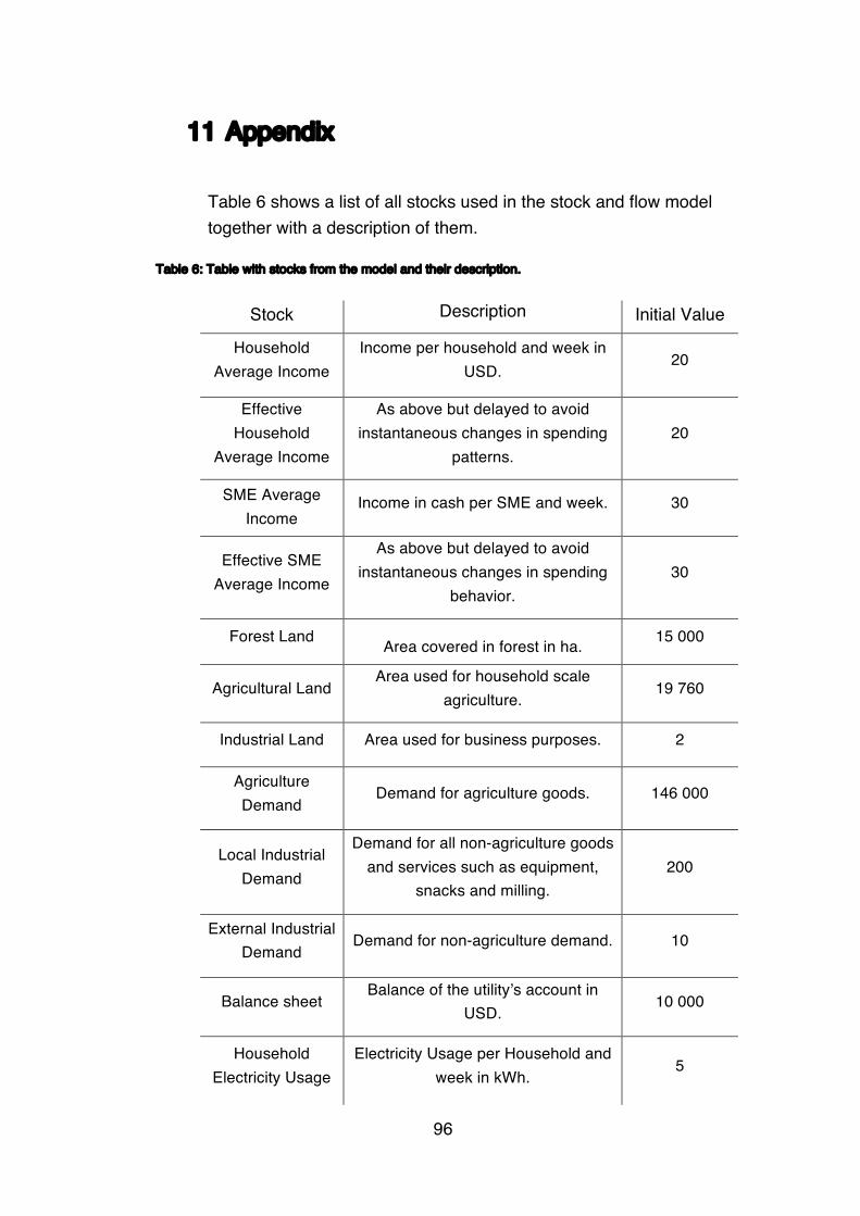
96

11   Appendix

Table 6 shows a list of all stocks used in the stock and flow model together with a description of them.

Table 6: Table with stocks from the model and their description.

Stock Description Initial Value

Household Average Income

Income per household and week in USD.

20

Effective Household

Average Income

As above but delayed to avoid instantaneous changes in spending

patterns. 20

SME Average Income

Income in cash per SME and week. 30

Effective SME Average Income

As above but delayed to avoid instantaneous changes in spending

behavior. 30

Forest Land Area covered in forest in ha. 15 000

Agricultural Land Area used for household scale

agriculture. 19 760

Industrial Land Area used for business purposes. 2

Agriculture Demand

Demand for agriculture goods. 146 000

Local Industrial Demand

Demand for all non-agriculture goods and services such as equipment,

snacks and milling. 200

External Industrial Demand

Demand for non-agriculture demand. 10

Balance sheet Balance of the utility’s account in

USD. 10 000

Household Electricity Usage

Electricity Usage per Household and week in kWh.

5

97

Stock Description Initial Value

SME Electricity Usage

Electricity Usage per SME and week in kWh.

80

Household Installed Load

Installed Household load in kW. 0.3

SME Installed Load

Installed SME load in kW. 1 or 29

Installed Capacity Installed generation capacity. 200

Planned Capacity Capacity planned to be built in kW. 0

Working Age Population Number of people in working age.

20 000

School Age Population Number of people in school.

2 000

Loan The utility’s debt in USD. 0

Technical Personnel

Amount of personnel who can do maintanence and connections.

2

Household non-Users

Number of households not connected to the miingrid.

3 520

Household Users Number of households connected to the minigrid.

600

SME non-Users Number of SMEs not connected to the minigrid.

130

SME Users Number of SMEs connected to the minigrid.

60

9 1 kW is used for the simulations with load limit and 2 kW for simulations

without load limit.

98

12   References

Ackoff, R. L. (1971). Towards a system of systems concepts. Management Science, 17(11), 661-671.

Adkins, E., Eapen, S., Kaluwile, F., Nair, G., & Modi, V. (2010). Off-grid energy services for the poor: Introducing LED lighting in the Millennium Villages Project in Malawi. Energy Policy, 38(2), 1087-1097. doi:http://dx.doi.org/10.1016/j.enpol.2009.10.061

Agoramoorthy, G., & Hsu, M. J. (2009). Lighting the lives of the impoverished in India’s rural and tribal drylands. Human Ecology, 37(4), 513-517.

Ahlborg, H. (2012). Electricity for better lives in rural Tanzania and Mozambique - Understanding and adressing the challanges. (Licenciate Thesis), Chalmers University of Technology.

Ahlborg, H. (2015). Walking along the lines of power: A systems approach to understanding the interplay between society, technology and nature in processes of rural electrification. (PhD), Chalmers University of Technology, Gothenburg.

Ahlborg, H., & Hammar, L. (2014). Drivers and barriers to rural electrification in Tanzania and Mozambique – Grid-extension, off-grid, and renewable energy technologies. Renewable Energy, 61(0), 117-124. doi:http://dx.doi.org/10.1016/j.renene.2012.09.057

Ahlborg, H., & Sjöstedt, M. (2015). Small-scale hydropower in Africa: Socio-technical designs for renewable energy in Tanzanian villages. Energy Research & Social Science, 5(0), 20-33. doi:http://dx.doi.org/10.1016/j.erss.2014.12.017

Al-Mas, S. (2010). Techno-economic Performance of Isolated Rural Power Systems: A Monte Carlo Simulation Approach. (PhD), Makerere University, Kampala.

Alexandra, N. (2010). Comparative Study on Rural Electrification Policies in Emerging Economies: OECD Publishing.

Bardhan, P., & Mookherjee, D. (2006). Decentralisation and Accountability in Infrastructure Delivery in Developing Countries*. The Economic Journal, 116(508), 101-127.

Bardi, U., El Asmar, T., & Lavacchi, A. (2013). Turning electricity into food: the role of renewable energy in the future of agriculture. Journal of Cleaner Production, 53, 224-231. doi:http://dx.doi.org/10.1016/j.jclepro.2013.04.014

Barlas, Y. (1989). Multiple tests for validation of system dynamics type of simulation models. European Journal of Operational Research, 42(1), 59-87. doi:http://dx.doi.org/10.1016/0377-2217(89)90059-3

Barlas, Y. (1996). Formal Aspects of Model Validity and Validation in System Dynamics. System Dynamics Review, 12(3), 183-210. doi:10.1002/(SICI)1099-1727(199623)12:3<183::AID-SDR103>3.0.CO;2-4

Barlas, Y., & Carpenter, S. (1990). Philosophical roots of model validation: Two paradigms. System Dynamics Review, 6(2), 148-166. doi:10.1002/sdr.4260060203

Barnes, D. (2007). The challenge of rural electrification: strategies for developing countries. Washington, DC: Routledge.

Barnes, D., & Foley, G. (2004). Rural Electrification in the Developing World: A Summary of Lesson from Successful Programs. ESMAP, World Bank.

Barton, J. P., & Infield, D. G. (2004). - Energy storage and its use with intermittent renewable energy. [- June 2004]. - 19(- 2), - 448.

99

Bertalanffy, L. v. (1968). General system theory: Foundations, development, applications: Braziller. New York.

Blum, N. U., Sryantoro Wakeling, R., & Schmidt, T. S. (2013). Rural electrification through village grids—Assessing the cost competitiveness of isolated renewable energy technologies in Indonesia. Renewable and Sustainable Energy Reviews, 22(0), 482-496. doi:http://dx.doi.org/10.1016/j.rser.2013.01.049

Cabraal, R. A., Barnes, D. F., & Agarwal, S. G. (2005). Productive uses of energy for rural development Annual Review of Environment and Resources (Vol. 30, pp. 117-144). Palo Alto: Annual Reviews.

Cecati, C., Citro, C., & Siano, P. (2011). Combined Operations of Renewable Energy Systems and Responsive Demand in a Smart Grid. [- Oct. 2011]. - 2(- 4), - 476.

Chakravorty, U., Pelli, M., & Ural Marchand, B. (2014). Does the quality of electricity matter? Evidence from rural India. Journal of Economic Behavior & Organization(0). doi:http://dx.doi.org/10.1016/j.jebo.2014.04.011

Chang, H.-S., & Zepeda, L. (2001). Agricultural productivity for sustainable food security in Asia and the Pacific: the role of investment. FAO ECONOMIC AND SOCIAL DEVELOPMENT PAPER, 75-92.

Chapman, L. J., & Chapman, J. (1971). STIMULUS/RESPONSE-TEST RESULTS ARE WHAT YOU THINK THEY ARE. Psychology Today, 5(6), 18-&.

Checkland, P. (2000). - Soft systems methodology: a thirty year retrospective. - 17(- S1), - S58. Retrieved from - http://dx.doi.org/10.1002/1099-1743(200011)17:1+<::AID-SRES374>3.0.CO;2-O

Chow, J., Kopp, R. J., & Portney, P. R. (2003). Energy resources and global development. Science, 302(5650), 1528-1531.

Cook, P. (2011). Infrastructure, rural electrification and development. Energy for Sustainable Development, 15(3), 304-313. doi:http://dx.doi.org/10.1016/j.esd.2011.07.008

Coombs, R., Saviotti, P., & Walsh, V. (1987). Economics and technological change: Rowman & Littlefield.

Cross, N., & Gaunt, C. T. (2003, 23-26 June 2003). Application of rural residential hourly load curves in energy modelling. Paper presented at the Power Tech Conference Proceedings, 2003 IEEE Bologna.

Davidsen, P. (1992). The structure-behavior diagram: understanding the relationship between structure and behavior in complex dynamic systems. Paper presented at the Proceedings of System Dynamics Conference.

Davis, B., Winters, P., Carletto, G., Covarrubias, K., Quiñones, E. J., Zezza, A., . . . DiGiuseppe, S. (2010). A Cross-Country Comparison of Rural Income Generating Activities. World Development, 38(1), 48-63. doi:http://dx.doi.org/10.1016/j.worlddev.2009.01.003

Díaz, P., Arias, C. A., Peña, R., & Sandoval, D. (2010). FAR from the grid: A rural electrification field study. Renewable Energy, - 35(- 12), - 2834. Retrieved from - http://www.sciencedirect.com/science/article/pii/S0960148110002235

Ebohon, O. J. (1996). Energy, economic growth and causality in developing countries: A case study of Tanzania and Nigeria. Energy Policy, 24(5), 447-453. doi:http://dx.doi.org/10.1016/0301-4215(96)00027-4

Eder, J. M., Mutsaerts, C. F., & Sriwannawit, P. (2015). Mini-grids and renewable energy in rural Africa: How diffusion theory explains adoption of electricity in Uganda. Energy Research & Social Science, 5, 45-54. doi:http://dx.doi.org/10.1016/j.erss.2014.12.014

Etymonline. Etymonline. Retrieved from http://www.etymonline.com/ Featherston, C. R., & Doolan, M. (2012). A Critical Review of the Criticisms of

System Dynamics. Paper presented at the Proceedings fo the 30th

100

International Conference of the System Dynamics Society, The 30th International Conference of the System Dynamics Society: St Gallen, Switzerland.

Fernando, C. Y., & Isaac, D. (2014). Assessing Sustainable Development of Isolated Communities: The Role of Electricity Supply. Paper presented at the International Conference of the System Dynamics Sociecity, Delft.

Flood, R., & Jackson, M. (1992). Creative Problem Solving: Total Systems Intervention. JOURNAL-OPERATIONAL RESEARCH SOCIETY, 43, 1013-1013.

Ford, A. (1997). System dynamics and the electric power industry. System Dynamics Review, 13(1), 57-85.

Forrester, J. (1971). Counterintuitive behavior of social systems. Theory and Decision, 2(2), 109-140. doi:10.1007/BF00148991

Forrester, J. W. (1961). Industrial dynamics. [Cambridge, Mass.: M.I.T. Press. François, C. (1999). Systemics and cybernetics in a historical perspective.

Systems Research and Behavioral Science, 16(3), 203-219. Freedman, D. A. (2005). Linear statistical models for causation: A critical

review. Encyclopedia of statistics in behavioral science. Frigg, R., & Hartmann, S. (2006). Models in science. Granger, C. W. (1988). Some recent development in a concept of causality.

Journal of econometrics, 39(1), 199-211. Hartvigsson, E., Ehnberg, J., Ahlgren, E., & Molander, S. (2015). Assessment

of Load Profiles in Minigrids: A Case in Tanzania. Paper presented at the International Universities Power Engineering Conference, Staffordshire University.

Hayden, F. G. (2006). The inadequacy of Forrester system dynamics computer programs for institutional principles of hierarchy, feedback, and openness. Journal of Economic Issues, 527-535.

Huang, B.-N., Hwang, M. J., & Yang, C. W. (2008). Causal relationship between energy consumption and GDP growth revisited: A dynamic panel data approach. Ecological Economics, 67(1), 41-54. doi:http://dx.doi.org/10.1016/j.ecolecon.2007.11.006

IEA. (2002). World Energy Outlook. Retrieved from IEA. (2015). World Energy Outlook. Retrieved from

http://www.worldenergyoutlook.org/media/weowebsite/energydevelopment/WEO2013Electricitydatabase.xlsx

IRENA. (2012). Renewable Energy Cost Analysis: Hydropower. Retrieved from

IRENA. (2015). Renewable Power Generation Costs 2014. Retrieved from Jackson, M. C. (1985). Social systems theory and practice: The need for a

critical approach. International Journal Of General System, 10(2-3), 135-151.

Jordan, R. (2013). Incorporating endogenous demand dynamics into long-term capacity expansion power system models for Developing countries. (Ph D), Massachusetts Institute of Technology, Engineering Systems Division. Retrieved from http://hdl.handle.net/1721.1/79547

Kahneman, D., & Tversky, A. (1977). Intuitive prediction: Biases and corrective procedures. Retrieved from

Kanase-Patil, A. B., Saini, R. P., & Sharma, M. P. (2010). Integrated renewable energy systems for off grid rural electrification of remote area. Renewable Energy, 35(6), 1342-1349. doi:http://dx.doi.org/10.1016/j.renene.2009.10.005

Kaundinya, D. P., Balachandra, P., & Ravindranath, N. H. (2009). Grid-connected versus stand-alone energy systems for decentralized power—A review of literature. Renewable and Sustainable Energy Reviews, 13(8), 2041-2050. doi:http://dx.doi.org/10.1016/j.rser.2009.02.002

101

Keys, P. (1990). System dynamics as a systems-based problem-solving methodology. Systems Practice, 3(5), 479-493.

Kirubi, C., Jacobson, A., Kammen, D. M., & Mills, A. (2009). Community-Based Electric Micro-Grids Can Contribute to Rural Development: Evidence from Kenya. World Development, 37(7), 1208-1221. doi:http://dx.doi.org/10.1016/j.worlddev.2008.11.005

Kolhe, M. L., Ranaweera, K. M. I. U., & Gunawardana, A. G. B. S. (2015). Techno-economic sizing of off-grid hybrid renewable energy system for rural electrification in Sri Lanka. Sustainable Energy Technologies and Assessments, 11, 53-64. doi:http://dx.doi.org/10.1016/j.seta.2015.03.008

Larsen, E. R., & Bunn, D. W. (1999). Deregulation in Electricity: Understanding Strategic and Regulatory Risk. The Journal of the Operational Research Society, 50(4), 337-344. doi:10.2307/3010451

Lee, C.-C. (2005). Energy consumption and GDP in developing countries: a cointegrated panel analysis. Energy Economics, 27(3), 415-427. Retrieved from http://ac.els-cdn.com/S014098830500023X/1-s2.0-S014098830500023X-main.pdf?_tid=0e85a272-9049-11e5-8cda-00000aab0f02&acdnat=1448108095_aa5db502db40a855a31ad4f335906a1c

Levin, T., & Thomas, V. M. (2014). Utility-maximizing financial contracts for distributed rural electrification. Energy, 69(0), 613-621. doi:http://dx.doi.org/10.1016/j.energy.2014.03.057

Ltd, O. H. C. (2006). Windfarm Construction: Economic Impact Appraisal Retrieved from

Maher, P., Smith, N. P. A., & Williams, A. A. (2003). Assessment of pico hydro as an option for off-grid electrification in Kenya. Renewable Energy, 28(9), 1357-1369. doi:http://dx.doi.org/10.1016/S0960-1481(02)00216-1

Manning, D. T., Means, P., Zimmerle, D., Galvin, K., Loomis, J., & Paustian, K. (2015). Using contingent behavior analysis to measure benefits from rural electrification in developing countries: an example from Rwanda. Energy Policy, 86, 393-401. doi:http://dx.doi.org/10.1016/j.enpol.2015.06.032

Mary, S. (1996). Bureaucrats in business : the economics and politics of government ownership. Retrieved from

Mashayekhi, A. N., Mohammadi, H., Mirassadollahi, K., & Kamranianfar, A. (2010). Modeling Sustainability of Renewable Energies in Rural Areas: A Case Study for Iran. Paper presented at the International Conference of the System Dynamics Society, Seoul, Korea.

Matinga, M. N., & Annegarn, H. J. (2013). Paradoxical impacts of electricity on life in a rural South African village. Energy Policy, 58(0), 295-302. doi:http://dx.doi.org/10.1016/j.enpol.2013.03.016

Michaelowa, K. (2000). Returns to education in low income countries: evidence for Africa. Committee on Developing Countries of the German Economic Association.

Milling, N. S. a. P. (2003). Modeling the Forest or Modeling the Trees - A comparision of System Dynamics and Agent-Based Simulation. International System Dynamics Conference. Retrieved from http://www.systemdynamics.org/conferences/2003/proceed/PAPERS/140.pdf

Mulder, P., & Tembe, J. (2008). Rural electrification in an imperfect world: A case study from Mozambique. Energy Policy, -36(8), 2785- 2794. Retrieved from - http://www.sciencedirect.com/science/article/pii/S030142150800236X

Neelsen, S., & Peters, J. (2011). Electricity usage in micro-enterprises—Evidence from Lake Victoria, Uganda. Energy for Sustainable Development, 15(1), 21-31.

102

Nfah, E. M., Ngundam, J. M., Vandenbergh, M., & Schmid, J. (2008). Simulation of off-grid generation options for remote villages in Cameroon. Renewable Energy, 33(5), 1064-1072. doi:http://dx.doi.org/10.1016/j.renene.2007.05.045

Nursebo, S., Peiyuan, C., Carlson, O., & Tjernberg, L. B. (2014). - Optimizing Wind Power Hosting Capacity of Distribution Systems Using Cost Benefit Analysis. [- June 2014]. - 29(- 3), - 1445.

OECD. (2011). Measuring Aid: 50 years of DAC statistics. Retrieved from Ozturk, I. (2010). A literature survey on energy–growth nexus. Energy Policy,

38(1), 340-349. doi:http://dx.doi.org/10.1016/j.enpol.2009.09.024 Palma-Behnke, R., Benavides, C., Lanas, F., Severino, B., Reyes, L., Llanos,

J., & Saez, D. (2013). A Microgrid Energy Management System Based on the Rolling Horizon Strategy. [- June 2013]. - 4(- 2), - 1006.

Paul, S., & Bhattacharya, R. N. (2004). Causality between energy consumption and economic growth in India: a note on conflicting results. Energy Economics, 26(6), 977-983. doi:http://dx.doi.org/10.1016/j.eneco.2004.07.002

Pellegrini, L., & Tasciotti, L. (2013). Rural electrification now and then: comparing contemporary challenges in developing countries to the USA's experience in retrospect. Paper presented at the Forum for Development Studies.

Pereira, M. G., Freitas, M. A. V., & da Silva, N. F. (2010). Rural electrification and energy poverty: Empirical evidences from Brazil. Renewable and Sustainable Energy Reviews, 14(4), 1229-1240. doi:http://dx.doi.org/10.1016/j.rser.2009.12.013

Peterson, T. (1992). Elkraften i Samhället: Ellagen 1902-1992: Svenska Elverksföreningen.

Qudrat-Ullah, H., & Davidsen, P. I. (2001). Understanding the dynamics of electricity supply, resources and pollution: Pakistan's case. Energy, 26(6), 595-606. doi:http://dx.doi.org/10.1016/S0360-5442(01)00019-6

Qudrat-Ullah, H., & Seong, B. S. (2010). How to do structural validity of a system dynamics type simulation model: The case of an energy policy model. Energy Policy, 38(5), 2216-2224. doi:10.1016/j.enpol.2009.12.009

Radzicki, M. J., & Tauheed, L. (2009). In Defense of System Dynamics: A Reply to Professor Hayden. Journal of Economic.

REN21. (2014). Renewables 2014 Global Status Report. Retrieved from Paris:

Rogers, E. M. (2010). Diffusion of innovations: Simon and Schuster. Roser, M. (2011). The number of people living in extreme poverty by world

region: 1981-2011. Sachs, J. (2005). The End of Poverty: How we can make it happen in our

lifetime: Penguin Group. Sarangi, G. K., Pugazenthi, D., Mishra, A., Palit, D., Kishore, V. V. N., &

Bhattacharyya, S. C. (2014). Poverty Amidst Plenty: Renewable Energy-Based Mini-Grid Electrification in Nepal. In S. C. Bhattacharyya & D. Palit (Eds.), Mini-Grids for Rural Electrification of Developing Countries: Analysis and Case Studies from South Asia (pp. 343-371).

Schnitzer, D., Lounsbury S., D., Carvallo, J. P., Deshmukh, R., Apt, J., & Kammen M., D. (2014). Microgrids for Rural Electrification: A critical review of best practices based on seven case studies. Retrieved from

Schoderbek, P. P. (1990). Management systems : conceptual considerations / Peter P. Schoderbek, Charles G. Schoderbek, Asterios G. Kefalas. Homewood, Ill: BPI/Irwin.

Senge, P. M. (1980). Tests for building confidence in system dynamics models. System dynamics, TIMS studies in management sciences, 14, 209-228.

103

Shete, M., & Rutten, M. (2015). Impacts of large-scale farming on local communities’ food security and income levels – Empirical evidence from Oromia Region, Ethiopia. Land Use Policy, 47, 282-292. doi:http://dx.doi.org/10.1016/j.landusepol.2015.01.034

Simon, H. A. (1996). The sciences of the artificial (Vol. 136): MIT press. Simon, H. A. (1996). The sciences of the artificial (3rd ed.): MIT Press. Solow, R. (1972, March 13) Unknown. Newsweek. Steel, K. (2008). Energy system development in Africa : the case of grid and

off-grid power in Kenya. (Ph D), Massachusetts Institute of Technology, Engineering Systems Division. Retrieved from http://hdl.handle.net/1721.1/43840

Sterman, J. D. (1984). Appropriate summary statistics for evaluating the historical fit of system dynamics models. Dynamica, 10(2), 51-66.

Sterman, J. D. (1991). A skeptic’s guide to computer models. Managing a nation: The microcomputer software catalog, 2, 209-229.

Sterman, J. D. (2000). Business dynamics: systems thinking and modeling for a complex world (Vol. 19): Irwin/McGraw-Hill Boston.

Sterman, J. D. (2002). All models are wrong: reflections on becoming a systems scientist. System Dynamics Review, 18(4), 501-531.

Tenenbaum, B., Greacen, C., Siyambalapitya, T., & Knuckles, J. (2014). From the Bottom Up - How Small Power Producers and Mini-grids Can Deliver Electrification and Renewable Energy in Africa. The World Bank.

Teufel, F., Miller, M., Genoese, M., & Fichtner, W. (2013). Review of System Dynamics models for electricity market simulations.

The White House. (2013). Power Africa [Press release]. Retrieved from http://www.whitehouse.gov/the-press-office/2013/06/30/fact-sheet-power-africa

The World Bank. (2008). The Welfare Impact of Rural Electrification (T. W. B. Group Ed.): IEG.

Tversky, A., & Kahneman, D. (1974). Judgment under uncertainty: Heuristics and biases. Science, 185(4157), 1124-1131.

UN. (2014). World Urbanization Prospects: The 2014 Revision. Retrieved from

UNDP. (2014). Human Development Report: Sustaining Human Progress: Reducing Vulnerabilities and Building Resilience. Retrieved from

Urpelainen, J. (2014). Grid and off-grid electrification: An integrated model with applications to India. Energy for Sustainable Development, 19, 66- 71. Retrieved from - http://www.sciencedirect.com/science/article/pii/S0973082613001142

Wamukonya, N., & Davis, M. (2001). Socio-economic impacts of rural electrification in Namibia: comparisons between grid, solar and unelectrified households. Energy for Sustainable Development, 5(3), 5-13. doi:http://dx.doi.org/10.1016/S0973-0826(08)60272-0

Watson, V. (2014). African urban fantasies: dreams or nightmares? Environment and Urbanization, 26(1), 215-231. doi:10.1177/0956247813513705

Williams, N. J., Jaramillo, P., Taneja, J., & Ustun, T. S. (2015). Enabling private sector investment in microgrid-based rural electrification in developing countries: A review. Renewable and Sustainable Energy Reviews, 52, 1268-1281. doi:http://dx.doi.org/10.1016/j.rser.2015.07.153

Von Bertalanffy, L. (1956). General system theory. General systems, 1(1), 11-17.

Zhang, L. a. C., X. (2012). A System Dynamics Study of the Development of Rural Energy in Shandong Province Civil Engineering and Urban Planning 2012 (pp. 62-68).

104