a test of the ohlson (1995) model: empirical evidence from...

A test of the Ohlson (1995) model:

Empirical evidence from Japan

Koji Ota*

Department of Commerce, Burgmann College, Kansai University Graduate School,

GPO Box 1345, Canberra ACT 2601, Australia

Abstract

This paper investigates the validity of the Ohlson [Contemp. Account. Res. 11 (1995) 661]

information dynamics (Linear Information Model: LIM) and attempts to improve the LIM. The

difficulty concerning the empirical tests of the LIM lies in identifying nt, which denotes information

other than abnormal earnings. Recent papers, such as those of Myers [Account. Rev. 74 (1999) 1],

Hand and Landsman [The pricing of dividends in equity valuation. Working paper, University of

North Carolina, 1999], and Barth et al. [Accruals, cash flows, and equity values. Working paper

(January) (July), Stanford University, 1999], all try to specify nt by using various accounting

information. Instead of tackling this difficult task, this paper focuses on serial correlation in the error

terms caused by omitting the necessary variable nt from the regression equation. The results indicate

that adjustment for serial correlation leads to an improvement of the LIM. D 2002 University of

Illinois. All rights reserved.

Keywords: Ohlson (1995) model; Information dynamics; Other information nt; Serial correlation; Durbin’s

alternative test; GLS

1. Introduction

The work of Ohlson (1995) has attracted considerable attention among accounting re-

searchers since its publication. This seminal paper consists of two main parts: the residual

0020-7063/02/$ – see front matter D 2002 University of Illinois. All rights reserved.

PII: S0020 -7063 (02 )00150 -4

* Tel.: +81-6-63690320.

E-mail address: [email protected] (K. Ota).

The International Journal of Accounting

37 (2002) 157–182

income valuation model (RIV) and the linear information dynamics. The RIV expresses firm

value as the sum of the book value of equity and the present value of future abnormal

earnings.1 However, the RIV is an application of the Dividend Discount Model and its

development cannot be attributed to Ohlson (1995).2 Both Dechow, Hutton, and Sloan (1999)

and Lo and Lys (2000) point out that the real contribution of Ohlson comes from his modeling

of the linear information dynamics.

The linear information dynamics attempts to identify the mechanism of abnormal

earnings and links current information to future abnormal earnings, which allows the

development of a valuation model of a firm. However, empirical testing of the Ohlson

(1995) linear information dynamics (the Linear Information Model: hereafter LIM) is not

easy, because the LIM contains the troublesome variable nt. This variable denotes

information other than abnormal earnings that has yet to be captured in current financial

statements but affects future abnormal earnings. It is often unobservable or very difficult

to observe because of its inherent properties. However, nt plays an integral role in the

LIM and seems to hold the key to the improvement of the LIM. Recent papers,

therefore, attempt to specify nt by using a number of accounting variables (e.g., Barth,

Beaver, Hand, & Landsman, 1999; Dechow et al., 1999; Hand & Landsman, 1998, 1999;

Myers, 1999).

This paper tries to improve the Ohlson (1995) LIM without tackling the difficult task of

specifying other information nt. The Ohlson (1995) LIM assumes that nt follows a first-orderautoregressive process, AR(1). Omitting this AR(1) variable, nt, from regression equations

will cause serial correlation in the regression error terms. Based on this presumption, the

error-term serial correlation is tested using Durbin’s alternative statistics. Serial correlation is

detected in about 40% of the sample. The problem of serial correlation in the error terms is

rectified by using generalized least squares (GLS). The results generate some improvement in

the Ohlson (1995) LIM. This modified LIM is also tested using stock market data. The results

of the tests generally support the superiority of the modified LIM over other LIMs that omit

the other information term, nt.In addition, the results of this research reveal some interesting similarities to those reported

in Barth et al. (1999), Dechow et al. (1999), and Hand and Landsman (1998, 1999). The

persistence coefficient of abnormal earnings has almost the same value for each of the prior

studies and this paper. Further, the coefficient on book value of equity is negative in this

study, which is consistent with previous studies.

The remainder of this paper proceeds as follows. Section 2 reviews the RIV and the

LIM. Section 3 conducts empirical tests on the LIM. Section 4 derives the valuation

models of the LIMs with testing based on stock market data, and Section 5 concludes

the paper.

1 Abnormal earnings are defined as accounting earnings minus a charge for the cost of capital.2 See Lo and Lys (2000) and Palepu, Bernard, and Healy (1996, chap. 7-17) for the historic details of

the model.

K. Ota / The International Journal of Accounting 37 (2002) 157–182158

2. Background

2.1. Residual income valuation model

The Dividend Discount Model defines the value of a firm as the present value of the

expected future dividends.

Vt ¼X1i¼1

Et

dtþi

ð1þ rÞi

" #, ð1Þ

where Vt = value of a firm at date t; Et[dt + i] = the expected dividends received at date t + i;

r= the discount rate that is assumed to be constant.

The clean surplus concept dictates that entries to retained earnings are limited to record

only periodic earnings and dividends. Then, the relation between book value of equity,

earnings, and dividends can be expressed as follows.

bt ¼ bt�1 þ xt � dt, ð2Þ

where bt = book value of equity at date t; xt = earnings for period t; dt = dividends paid at date t.

Book value of equity at date t� 1 multiplied by the capital cost is considered ‘‘normal

earnings’’ of the firm. Then, earnings for the period t minus ‘‘normal earnings’’ can be

defined as ‘‘abnormal earnings.’’3

xat � xt � rbt�1, ð3Þ

where xta = abnormal earnings for period t.

Simple algebraic manipulation allows Eqs. (2) and (3) to be rewritten as:

dt ¼ xat þ ð1þ rÞbt�1 � bt:

Using this expression to replace dt + i in Eq. (1) yields the RIV,

Vt ¼ bt þX1i¼1

Et

xatþi

ð1þ rÞi

" #: ð4Þ

The RIV implies that a firm’s value equals its book value of equity and the present value of

anticipated abnormal earnings. One of the interesting properties of the RIV is that a firm’s

value based on the RIV will not be affected by accounting choices.4

4 See Lundholm (1995) and Palepu et al. (1996, chap. 7-5) for the details of this particular property of RIV.

3 The terminology is confusing. When it is incorporated into the valuation model, it is usually ‘‘residual

income,’’ such as ‘‘residual income valuation model’’. But, when it is referred to as earnings, it is either ‘‘residual

income’’ or ‘‘abnormal earnings’’. It seems that the term ‘‘abnormal earnings’’ is more commonly used. The terms

‘‘residual income valuation model’’ and ‘‘abnormal earnings’’ are used in this paper.

K. Ota / The International Journal of Accounting 37 (2002) 157–182 159

2.2. Linear information model

The LIM was originally proposed in Feltham and Ohlson (1995) and Ohlson (1995). The

LIM is an information dynamics model that describes the time-series behavior of abnormal

earnings. Dechow et al. (1999) emphasize that the real achievement of Feltham and Ohlson

(1995) and Ohlson (1995) is that the LIM creates a link between current information and a

firm’s intrinsic value.

2.2.1. Ohlson (1995) LIM

The Ohlson (1995) LIM assumes that the time-series behavior of abnormal earnings

follows:

xatþ1 ¼ !11xat þ nt þ "1tþ1, ð5aÞ

ntþ1 ¼ �nt þ "2tþ1, ð5bÞwhere xt

a = abnormal earnings for period t (xta� xt� rbt� 1); nt = information other than

abnormal earnings; !11 = persistence parameter of abnormal earnings xta (0�!11 < 1);

� = persistence parameter of other information nt (0� � < 1); "1t, "2t = error terms.

The Ohlson (1995) LIM assumes that the source of abnormal earnings is monopoly rents.

Although monopoly rents may persist for some time, market competition will force returns

toward the cost of capital in the long run. Therefore, the persistence parameter !11 is

predicted to lie in the range 0�!11 < 1.

Combining the RIV in Eq. (4) with the Ohlson (1995) LIM in Eqs. (5a) and (5b) yields the

following valuation function:5

Vt ¼ bt þ �1xat þ �1nt,

where

�1 ¼!11

1þ r � !11

�1 ¼1þ r

ð1þ r � !11Þð1þ r � �Þ :

2.2.2. Feltham and Ohlson (1995) LIM

Feltham and Ohlson (1995) assume the following four equations with some relabeling

for simplicity.6

xatþ1 ¼ !11xat þ !12bt þ n1t þ "1tþ1, ð6aÞ

5 See Ohlson (1995), Appendix 1, for the demonstration of this result.6 Although Feltham and Ohlson (1995) use operating assets and operating earnings instead of book value of

equity and earnings, both result in the same abnormal earnings. For further details, see Myers (1999, Note 6) and

Penman and Sougiannis (1998, pp. 350–351).


btþ1 ¼ !22bt þ n2t þ "2tþ1, ð6bÞ

n1tþ1 ¼ �1n1t þ "3tþ1, ð6cÞ

n2tþ1 ¼ �2n2t þ "4tþ1, ð6dÞ

where !11 = persistence parameter of abnormal earnings xta; (0�!11 < 1); !12 = conservatism

parameter (0�!12); !22 = growth parameter of book value of equity (0�!22 < 1 + r); n1t,n2t = information other than abnormal earnings; �1, �2 = persistence parameter of n1t and n2t,respectively (0� �1, �2 < 1); "1t, "2t, "3t, "4t = error terms.

The Feltham and Ohlson (1995) LIM assumes that abnormal earnings are generated from

two sources. The first source is monopoly rents. Since market competition is expected to

force returns toward the cost of capital in the long run, !11 is predicted to lie in the range

0�!11 < 1. The second source is accounting conservatism. Accounting conservatism

generally depresses the valuation of assets below their market value, which generates

abnormal earnings that can be calculated by multiplying the difference between market

value and book value of equity by the cost of capital. Therefore, under conservative

accounting, !12 is predicted to be 0�!12.7

Combining the RIV in Eq. (4) with the Feltham and Ohlson (1995) LIM in Eqs. (6a)–(6d)

yields the following valuation function:8

Vt ¼ bt þ �1xat þ �2bt þ �1n1t þ �2n2t,

where

�1 ¼!11

1þ r � !11

, �2 ¼ð1þ rÞ!12

ð1þ r � !11Þð1þ r � !22Þ,

�1 ¼1þ r

ð1þ r � !11Þð1þ r � �1Þ, �2 ¼

ð1þ rÞ!12

ð1þ r � !11Þð1þ r � !22Þð1þ r � �2Þ:

Thus, the Feltham and Ohlson (1995) LIM and the Ohlson (1995) LIM allow us to obtain

the valuation functions of a firm without requiring either explicit forecasts of future dividends

or additional assumptions about the calculation of terminal value. However, whether or not

the LIM characterizes reality with reasonable accuracy is purely an empirical matter.

In the next section, I test the validity of the Ohlson (1995) LIM and the Feltham and

Ohlson (1995) LIM after transforming them to empirically testable forms.

8 See appendix in Feltham and Ohlson (1995) for the demonstration of this result.

7 Feltham andOhlson (1995) characterize (0 <!12) as conservative accounting, (0 =!12) as unbiased accounting,

and (0 >!12) as aggressive accounting.


3. Empirical tests on LIM

3.1. Model development

3.1.1. LIM1 and LIM2: based on the Ohlson (1995) model

It is challenging to test the Ohlson (1995) LIM in Eqs. (5a) and (5b) without any

modification, because other information nt is unobservable or difficult to measure. Therefore,

LIM1 assumes nt to be zero and omits it from the model. However, omitting a relevant

variable, just because it is unobservable, leads to model misspecification. Therefore, LIM2

assumes nt to be a constant. The parameters of the models LIM1 and LIM2 are estimated

using OLS regression.

LIM1 : xatþ1 ¼ !11xat þ "tþ1

LIM2 : xatþ1 ¼ !10 þ !11xat þ "tþ1

3.1.2. LIM3 and LIM4: based on the Feltham and Ohlson (1995) model

Again, estimating the Feltham and Ohlson (1995) LIM in Eqs. (6a)–(6d) without any

modification is difficult, because it contains other information n1t, which is unobservable.

Therefore, LIM3 assumes n1t to be zero, and LIM4 assumes n1t to be a constant. The

parameters of LIM3 and LIM4 are estimated by OLS using the following forms:

LIM3 : xatþ1 ¼ !11xat þ !22bt þ "tþ1

LIM4 : xatþ1 ¼ !10 þ !11xat þ !22bt þ "tþ1

3.1.3. LIM5 and LIM6: higher-order autoregression of xta

The Ohlson (1995) LIM assumes that abnormal earnings xta is the first-order autore-

gressive process AR(1). However, in reality, abnormal earnings xta might follow a higher-

order autoregressive process AR(p). It is possible that the next-period abnormal earnings

are affected not only by current-period abnormal earnings but also by past-period

abnormal earnings. Therefore, LIM5 examines the second-order autoregressive process

of abnormal earnings AR(2), and LIM6 examines the third-order autoregressive process of

abnormal earnings AR(3). The parameters of LIM5 and LIM6 are estimated by OLS.

LIM5 : xatþ1 ¼ !11xat þ !12x

at�1 þ "tþ1

LIM6 : xatþ1 ¼ !11xat þ !12x

at�1 þ !13x

at�2 þ "tþ1


3.1.4. LIM7: serial correlation in the error terms

The models, LIM1–6, are all based on the assumption of nt being zero or a constant

because of the difficulty in specifying nt. However, omitting a necessary variable just because

it is unobservable may lead to misspecification of the LIM causing nt to be absorbed in the

error term. As can be seen in Eqs. (5b) and (6c), both Ohlson (1995) and Feltham and Ohlson

(1995) assume that nt follows a first-order autoregressive process with 0� � < 1. If this

assumption is true, the residuals of LIM1–6 would show positive serial correlation.

The Durbin–Watson (DW) test is employed to examine serial correlation in the error terms

of LIM1–6. However, the DW test should not be used when there is no constant term in the

model, and its statistic is known to exhibit a bias toward 2 when lagged dependent variables

are included as regressors (Johnston & DiNardo, 1997, pp. 178–184). To guard against these

problems, the Durbin’s alternative test is primarily used.

Hypothesis testing for serial correlation in the error terms is:

H0 : utþ1 ¼ �ut þ "tþ1 � ¼ 0

H1 : utþ1 ¼ �ut þ "tþ1 � > 0:

The null hypothesis is that there is no serial correlation in the error terms and the alternative

hypothesis is that there is positive serial correlation in the error terms.

LIM7 is a modified version of LIM1 and corrects serially correlated errors. Therefore, only

a portion of the LIM1 sample, the part significant under the Durbin’s alternative test,

comprises the sample for LIM7. The parameters of LIM7 are estimated using a generalized

least squares grid-search method (GLS-GRID).9

LIM7 : xatþ1 ¼ !11xat þ utþ1 and utþ1 ¼ �ut þ "tþ1:

3.2. Data

3.2.1. Sample selection

The sample selection requirements are as follows:

(i) the firms are listed on the Tokyo Stock Exchange (TSE) or Osaka Stock Exchange

(OSE),

(ii) the accounting period ends in March,

(iii) banks, securities firms, and insurance firms are excluded,

(iv) a minimum of 27 consecutive years of accounting data is available for each firm

included in the sample, and

(v) book value of equity is not negative in any year.

9 The maximum likelihood method (ML) is commonly used to deal with the problem of serial correlation in

the error terms. However, ML is known to have a small sample bias when lagged endogenous variables are

included in the model. Therefore, GLS is used in this paper.


The data source is NIKKEI-ZAIMU DATA. As of March 1998, there were 1705 firms that

met requirements (i), (ii), and (iii), of which 750 firms also satisfy requirement (iv).

Requirement (v) reduces the sample to 674 firms.10

The parameters for each of the LIMs for each firm are estimated from the earliest year in

which data are available to years ending 1991 to 1998. For example, Fujitsu’s accounting data

are available for 35 years since 1964. First, the parameters of LIM1–7 are estimated using data

from1964 to 1991.Next, the parameters of LIM1–7 are estimated using data from1964 to 1992,

then from 1964 to 1993, and so on, until 1998. Thus, eight sets of parameters of LIM1–7 are

estimated for the periods 1964–1991, 1964–1992, 1964–1993, 1964–1994, 1964–1995,

1964–1996, 1964–1997, and 1964–1998. Requirement (iv) guarantees that the parameters are

estimated using at least 18 years of necessary data. Requirement (v) is necessary because firms

with negative book value of equity generate negative normal earnings.

Panel A of Table 1 presents the number of years of historical accounting data available.

The weighted average is 33.6 years. Panel B of Table 1 presents the stock markets on which

10 This 27-year requirement limits the generality of this paper because of potential survivorship bias. There is a

tradeoff between stable parameters and survivorship bias. This problem is discussed in Morel (1999, Note 7).

Table 1

Sample firms

Panel A: Data years of sample firmsa

Available data years No. of firms %

27 years 6 0.9

28 years 46 6.8

29 years 30 4.5

30 years 9 1.3

31 years 3 0.4

32 years 5 0.7

33 years 7 1.0

34 years 294 43.6

35 years 274 40.7

Total 674 100.0

Panel B: Stock markets listedb

Stock Market No. of firms %

TSE, first section 503 74.6

TSE, second section 116 17.2

OSE, first section 18 2.7

OSE, second section 37 5.5

Total 674 100.0a Available data years for 674 sample firms. Data source is NIKKEI-ZAIMU DATA.b TSE and OSE stand for Tokyo Stock Exchange and Osaka Stock Exchange. The first section has more

stringent criteria for listing than the second section. Therefore, the first section usually lists bigger firms than the

second section.


sample firms are listed as of March 1998. About three-quarters of the sample firms are listed

on the TSE first section. Thus, the sample firms for which the LIM is appropriate are likely to

be large firms. The question of whether the selected sample represents a fair cross-section of

Japanese firms remains unsolved, though the study certainly provides insight into the impact

on large Japanese firms.

3.2.2. Estimating the cost of capital and the computation of abnormal earnings

In defining abnormal earnings, most prior research uses a constant discount rate of 12% or

an industry risk premium estimated by using methods similar to those reported in Fama and

French (1997). One of the few exceptions is Abarbanell and Bernard (2000) in which beta

(CAPM) is used to allow for the time-varying and firm-specific discount rate. Following

Abarbanell and Bernard, the discount rate is estimated for each firm-year.

rjt ¼ rft þ �jt½0:02,

where rjt = estimated cost of capital for firm j in May of year t; rft = an interest rate of long-

term national bonds (10 years) in May of year t;11 �jt = estimated CAPM beta for firm j in

May of year t.

The CAPM beta is estimated using a rolling regression procedure with a 60-month window

against the NIKKEI 225 Index.12 The market risk premium is assumed to be 2%. The results

presented later are qualitatively similar whenmarket risk premium is assumed to be 4% and 6%.

The computation of abnormal earnings is as follows. (After this subsection, subscript j,

which denotes a sample firm, will be omitted for ease of exposition.)

xajt � xjt � rjtbjt�1,

where xjt = income before extraordinary items, net of tax, for firm j for period t; rjt = estimated

cost of capital for firm j in May of year t; bjt = book value of equity for firm j at date t.

Strictly speaking, excluding extraordinary items from net income violates the clean surplus

relation that underlies the theoretical development of RIV. However, including extraordinary

items in the calculation of abnormal earnings makes the estimation of the LIM unstable due to

their nonrecurring nature. Therefore, consistent with many prior studies in the United States,

income before extraordinary items, net of tax, is used instead of net income.13 Moreover, tax

applicable to extraordinary items is not reported in the income statement in Japan, so income

before extraordinary items, net of tax, is estimated using the formula below.

ECO ðnet of taxÞt ¼ ECOt � f1� ðCorpTRt þ ResidentTRtÞg ðt ¼ 1964� 1998Þ,

13 See Barth et al. (1999), Dechow et al. (1999), Hand and Landsman (1998, 1999), and Myers (1999) for

further discussion.

12 Where monthly returns are not available for 60 months, due to the lack of stock price data, the beta is

assumed to be equal to one.

11 Since 10-year national bonds are not available before 1971, 7-year national bonds are used before 1971 and

government-guaranteed bonds are used before 1965.


where ECOt = earnings from continuing operations for year t; CorpTRt = corporation tax rate

for year t; ResidentTRt = residents’ tax rate for year t.14

3.3. Results of LIM1–7

3.3.1. Descriptive statistics

Table 2 presents descriptive statistics for each of the variables used in estimating LIM1–7.

The mean (median) abnormal earnings over the sample period is ¥37.1 (31.9) million

given an assumed market risk premium of 2%. When the 4% and the 6% market risk

premium are used, abnormal earnings become predominantly negative with the mean

(median) of � ¥669.5 (� 44.9) million and � ¥1376.1 (� 137.1) million, respectively.

Table 2 also reveals that the mean (median) estimated cost of capital over the sample period is

7.95% (8.80%).

3.3.2. Results of LIM1–6

Panels A and B of Table 3 report the results for LIM1 and LIM2, respectively. As

predicted, the persistence coefficients on abnormal earnings, !11, are positive and their t

statistics are statistically significant in both LIM1 and LIM2. The estimates of !11 for LIM1

and LIM2 are 0.73 and 0.67, respectively, both of which are comparable with prior research

in the US.15 The coefficient, !10, is a constant in LIM2 and it is not statistically significant.

The assumption of LIM2 that other information nt is a constant, does not seem to be

appropriate. The fact that both DW statistics and Durbin’s alternative statistics calculated with

LIM2 are worse than those of LIM1 supports this view. Other information nt does not appearto be absorbed in a constant. The Adj. R2 for LIM1 and LIM2 is .43 and .41, respectively.

These values, however, cannot be compared unconditionally, because LIM1 is the regression

equation with no constant term. Still, there does not seem to be much difference between

LIM1 and LIM2 in terms of Adj. R2.16

Panels C and D of Table 3 report the results of LIM3 and LIM4, respectively. Both Panels

C and D reveal negative coefficients on book value of equity, !22, though they are not

statistically significant. As explained in Section 2.2, the coefficient on book value of equity

!22 is predicted to take a positive value under conservative accounting. The finding in this

14 Residents’ tax is levied by local municipalities. The rate differs across regions. The standard tax rate is used

in this study. Corporation business tax is ignored, because it was included in general and administrative expenses

until 1999.

16 In estimating the regression equation with no constant term, R2 requires special attention. In the case of

LIM1, R2 can be defined as eitherP

xta2/P

xta2 or the correlation coefficient of xt

a and xta. The latter definition of

R2 is used in this paper, because R2 is the correlation coefficient of xta and xt

a with or without a constant term.

Therefore, the comparison of the competing models is possible at least from this perspective. The meaning of the

Adj. R2 in regression equations will vary depending on whether the model includes a constant term or not.

15 The persistence parameter !11 in LIM2 is 0.62 in Dechow et al. (1999) and 0.66 in Barth et al. (1999). The

Adj. R2 is .34 and .40, respectively.


paper is not consistent with current conservative accounting practice. Similar results are

reported in prior US research and they are statistically significant.17

The sample used in this study is limited to large firms that have been in operation for a

long time. Since large Japanese firms tend to possess land and securities that were acquired a

long time ago, these assets are recorded at historical costs and should depress the book value

of equity, which generates abnormal earnings. Therefore, !22 is predicted to be positive in this

study in contrast to the US studies that reports a negative coefficient. However, the finding

here does not support this theory.

The coefficient on abnormal earnings, !11, is positive in both LIM3 and LIM4 and their t

statistics are statistically significant. The coefficient !10 is a constant in LIM4 and is not

statistically significant. The Adj. R2 for LIM3 and LIM4 is .47, which indicates a slight

improvement compared with the Adj. R2 of LIM1 and LIM2. However, considering that the

number of explanatory variables is increased in LIM3 and LIM4, the difference is statistically

small. After all, no improvement is observed by adding book value of equity, bt, to LIM1 and

LIM2 as an explanatory variable.

Panels E and F of Table 3 indicate that the results for LIM5 and LIM6 are similar to those

for LIM1–4, which show that only !11 is statistically significant. Still, one noticeable finding

is that both DW statistics and Durbin’s alternative statistics show no evidence of statistically

significant serial correlation in the error terms in LIM5 and LIM6. The negative sign of !12 is

also noteworthy. An explanation for these findings is as follows.

The Ohlson (1995) model assumes

xatþ1 ¼ !11xat þ nt þ "1tþ1 ð0 � !11 < 1Þ, ð5aÞ

ntþ1 ¼ �nt þ "2tþ1 ð0 � � < 1Þ: ð5bÞ

Table 2

Descriptive statistics on variables, 1965–1998 (in ¥ millions)a

Description Variable Mean

Standard

deviation 1Q Median 3Q

Book value of equity b 38,482 105,153 2603 8426 29,404

Net income x 2840 8497 180 666 2171

Abnormal earnings xa 37.1 4964.0 � 339.9 31.9 399.0

Cost of capital (%) r 7.95 1.95 6.42 8.80 9.13a Each variable has a total of 21,986 firm-year observations.

17 In this study, the estimate of !22 and its (t statistic) in LIM4 are � 0.03 (� 1.54). Hand and Landsman

(1998) report � 0.02 (� 2.6), Myers (1999) reports � 0.005 (t statistic unknown), Dechow et al. (1999) report

� 0.09 (� 77.64), Hand and Landsman (1999) report � 0.006 (� 1.4), and Barth et al. (1999) report � 0.07

(� 7.81).


However, nt is ignored in LIM1: xt + 1a =!11xt

a + "t + 1 because it is unobservable. Then, ntwill be absorbed in the error term in LIM1. Since nt is assumed to be the first-order

autoregressive process, the error terms in LIM1 would be serially correlated as follows:

xatþ1 ¼ !11xat þ utþ1, ð7aÞ

utþ1 ¼ �ut þ "tþ1 ð0 � � < 1Þ: ð7bÞRewriting Eq. (7a) at date t� 1 as

xat ¼ !11xat�1 þ ut: ð7cÞ

Multiplying Eq. (7c) by �, then subtracting the equation from Eq. (7a) yields

xatþ1 � �xat ¼ !11ðxat � �xat�1Þ þ utþ1 � �ut: ð7dÞ

Table 3

Results of LIM1–6 estimationa

(Panel A) LIM1: xt + 1a =!11xt

a + "t + 1

!11 DW D-alt Adj. R2

Mean

(t-stat)

0.73

(6.06)

1.62 1.28 .43

(Panel B) LIM2: xt + 1a =!10 +!11xt

a + "t + 1

!10 !11 DW D-alt Adj. R2

Mean

(t-stat)

12.9

(� 0.09)

0.67

(4.95)

1.61 1.46 .41

(Panel C) LIM3: xt + 1a =!11xt

a +!22bt + "t + 1


Mean

(t-stat)

0.63

(4.34)

� 0.01

(� 1.04)

1.63 1.44 .47

(Panel D) LIM4: xt + 1a =!10 +!11xt

a +!22bt + "t + 1

!10 !11 !22 DW D-alt Adj. R2

Mean

(t-stat)

445.6

(1.20)

0.58

(3.79)

� 0.03

(� 1.54)

1.64 1.49 .47

(Panel E) LIM5: xt + 1a =!11xt

a +!12xt� 1a + "t + 1


Mean

(t-stat)

0.90

(4.63)

� 0.26

(� 1.28)

1.92 0.06 .47

(Panel F) LIM6: xt + 1a =!11xt

a +!12xt � 1a +!13xt� 2

a + "t + 1

!11 !12 !13 DW D-alt Adj. R2

Mean

(t-stat)

0.90

(4.24)

� 0.28

(� 0.93)

0.04

(0.18)

1.93 0.00 .47

a A total of 5392 estimated parameters and t statistics are obtained from 674 sample firms for 8 years from

1991 to 1998. Figures in the table are the mean of the 5392 estimated parameters and t statistics. DW and D-alt.

denote the Durbin–Watson statistic and Durbin’s alternative statistic.


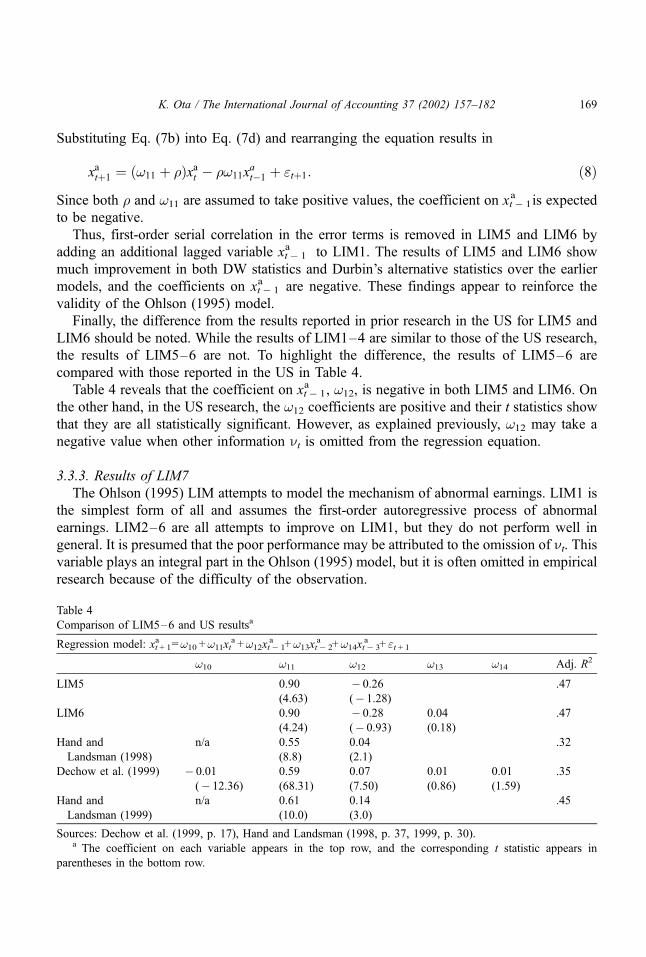
Substituting Eq. (7b) into Eq. (7d) and rearranging the equation results in

xatþ1 ¼ ð!11 þ �Þxat � �!11xat�1 þ "tþ1: ð8Þ

Since both � and !11 are assumed to take positive values, the coefficient on xt� 1a is expected

to be negative.

Thus, first-order serial correlation in the error terms is removed in LIM5 and LIM6 by

adding an additional lagged variable xt� 1a to LIM1. The results of LIM5 and LIM6 show

much improvement in both DW statistics and Durbin’s alternative statistics over the earlier

models, and the coefficients on xt� 1a are negative. These findings appear to reinforce the

validity of the Ohlson (1995) model.

Finally, the difference from the results reported in prior research in the US for LIM5 and

LIM6 should be noted. While the results of LIM1–4 are similar to those of the US research,

the results of LIM5–6 are not. To highlight the difference, the results of LIM5–6 are

compared with those reported in the US in Table 4.

Table 4 reveals that the coefficient on xt� 1a , !12, is negative in both LIM5 and LIM6. On

the other hand, in the US research, the !12 coefficients are positive and their t statistics show

that they are all statistically significant. However, as explained previously, !12 may take a

negative value when other information nt is omitted from the regression equation.

3.3.3. Results of LIM7

The Ohlson (1995) LIM attempts to model the mechanism of abnormal earnings. LIM1 is

the simplest form of all and assumes the first-order autoregressive process of abnormal

earnings. LIM2–6 are all attempts to improve on LIM1, but they do not perform well in

general. It is presumed that the poor performance may be attributed to the omission of nt. Thisvariable plays an integral part in the Ohlson (1995) model, but it is often omitted in empirical

research because of the difficulty of the observation.

Table 4

Comparison of LIM5–6 and US resultsa

Regression model: xt + 1a =!10 +!11xt

a +!12xt� 1a +!13xt� 2

a +!14xt� 3a + "t + 1

!10 !11 !12 !13 !14 Adj. R2

LIM5 0.90

(4.63)

� 0.26

(� 1.28)

.47

LIM6 0.90

(4.24)

� 0.28

(� 0.93)

0.04

(0.18)

.47

Hand and

Landsman (1998)

n/a 0.55

(8.8)

0.04

(2.1)

.32

Dechow et al. (1999) � 0.01

(� 12.36)

0.59

(68.31)

0.07

(7.50)

0.01

(0.86)

0.01

(1.59)

.35

Hand and

Landsman (1999)

n/a 0.61

(10.0)

0.14

(3.0)

.45

Sources: Dechow et al. (1999, p. 17), Hand and Landsman (1998, p. 37, 1999, p. 30).a The coefficient on each variable appears in the top row, and the corresponding t statistic appears in

parentheses in the bottom row.


However, as nt does seem to hold the key to the improvement of the LIM, recent research

in the US attempts to specify nt. Myers (1999) uses order backlog, Hand and Landsman

(1998, 1999) use dividends, Barth et al. (1999) use accruals and cash flows, and Dechow

et al. (1999) use the absolute value of abnormal earnings, the absolute value of special

accounting items, the absolute value of accounting accruals, dividends, an industry-specific

variable, and analysts’ earnings forecasts as proxies for nt. In this paper, LIM1 is adjusted to

remove serial correlation from the residuals. In effect, LIM7 tries to circumvent the difficulty

of specifying nt by correcting serial correlation in the error terms in LIM1 that could arise

from the omission of nt.Durbin’s alternative statistic is used to test for serial correlation in the errors. The

significance level is 5% using a one-tailed test.18 Table 5 shows that, of the entire sample

of 5392 firm-year observations in LIM1, 2102 observations are significant in the test for

serial correlation, which is about 40% of the entire sample.19 Panel A of Table 6 shows

the results of estimating the parameters of LIM7 by GLS-GRID using the 2102

observations. To highlight the difference between LIM7 and LIM1, the results of LIM1

estimation using the same 2102 observations are shown in Panel B of Table 6. The Adj.

R2 increases from .48 in LIM1 to .53 in LIM7, and Durbin’s alternative statistic also

improves from 2.71 in LIM1 to 0.09 in LIM7 indicating that serial correlation is removed

from the error terms.

Table 5

Number of LIM1 observations that are significant in tests of serial correlation in the errorsa

Estimation years No. of observations No. of AR(1) observations %

1965–1991 674 188 27.9

1965–1992 674 253 37.5

1965–1993 674 272 40.4

1965–1994 674 274 40.7

1965–1995 674 272 40.4

1965–1996 674 286 42.4

1965–1997 674 285 42.3

1965–1998 674 272 40.4

Total 5392 2102 39.0a Durbin’s alternative statistic is used to test for serial correlation in LIM1 errors. The number of degrees of

freedom= the number of observations� 2, and the significance level is 5% using a one-tailed test.

19 Myers (1999) notes that the mean (median) DW statistic for LIM2 and LIM4 is 1.895 (1.942) and 1.937

(1.958), respectively, and there are few firms with DW statistics far from 2. These results are inconsistent with the

findings in this paper. One possible explanation for this inconsistency is that Myers used the DW statistic to test

for serial correlation in the error terms, which is known to have a bias toward 2 when lagged endogenous variables

are included in the models.

18 The Durbin’s alternative test is a test of the coefficient �1 in ut + 1 = �1ut + �2xt� 1a + "t + 1 in the case of LIM1.

Therefore, the number of degrees of freedom is the number of observations minus two.


3.4. Stationarity of abnormal earnings

Tests of the stationarity of abnormal earnings are of particular interest in the investiga-

tion of the validity of the Ohlson (1995) model. The Ohlson (1995) model assumes that

abnormal earnings converge eventually due to market competition. If abnormal earnings

follow a random-walk process, the validity of the Ohlson (1995) model is in doubt.

Therefore, the stationarity of abnormal earnings for the 674 firms is investigated using the

Augmented Dickey–Fuller (hereafter ADF) test. The problem of the ADF test is that the

actual data-generating process is unknown. Therefore, three types of unit root tests are

conducted in this paper:

ðNo Constant or TrendÞ Dxat ¼ �xat�1 þX4p¼2

�pDxat�pþ1 þ "t,

ðWith ConstantÞ Dxat ¼ �0 þ �xat�1 þX4p¼2

�pDxat�pþ1 þ "t,

ðWith Constant and TrendÞ Dxat ¼ �0 þ �1t þ �xat�1 þX4p¼2

�pDxat�pþ1 þ "t:

Column (i) of Table 7 shows the results of the ADF test on the stationarity of abnormal

earnings xta. Maximum lags are set at 3 and optimal lags are chosen using the AIC. The

column reveals that 61.7% of the sample firms reject the null hypothesis of a unit root at

the 10% level when neither constant nor time trend is added. However, when both a

constant and a time trend are added to the model, only 28.9% of the sample firms reject the

null of a unit root. This may be due to misspecification of the simpler model or it may be

Table 6

Results of LIM7 estimationa

(Panel A) LIM7: xt + 1a =!11xt

a + ut + 1, ut + 1 = �ut + "t + 1

!11 � DW D-alt Adj. R2

Mean

(t-stat)

0.52

(2.04)

0.50

(1.88)

1.72 0.09 .53

(Panel B) LIM1: xt + 1a =!11xt

a + "t + 1

!11 DW D-alt Adj. R2

Mean

(t-stat)

0.75

(6.27)

1.31 2.71 .48

a The comparison of the parameters between LIM1 and LIM7 with regard to the 2102 firm-year observations

in Table 5 is reported. Figures in the table are the mean of the 2102 estimated parameters and t statistics. DW and

D-alt denote the Durbin–Watson statistic and the Durbin’s alternative statistic.


due to the decrease in the degrees of freedom caused by adding extra regressors to the

model.20

First-differenced abnormal earnings Dxta are also tested for stationarity and the results

are shown in Column (ii) of Table 7. This reveals that 96.7% of the sample firms

reject the null hypothesis of a unit root at the 10% level when neither constant nor

time trend is added. Even when these are added, 71.2% of the sample firms reject the

null hypothesis.

Table 7

Stationarity of abnormal earnings using the ADF testa

(i) xta c (ii) Dxt

a c

Percentage of observations

rejected at the

Percentage of observations

rejected at the

Modelb10%

level

5%

level

10%

level

5%

level

t(No Constant or Trend)

61.7 44.5 96.7 93.6

tm(With Constant)

34.3 22.7 87.1 79.1

tt(With Constant and Trend)

28.9 19.7 71.2 54.2

Maximum lags are set at three and optimal lags are chosen using the AIC.a A total of 674 firms are used to test the stationarity of their abnormal earnings.b Three types of unit root tests are performed:

ðNo Constant or TrendÞ Dxat ¼ �xat�1 þX4p¼2

�pDxat�pþ1 þ "t ,

ðWith ConstantÞ Dxat ¼ �0 þ �xat�1 þX4p¼2

�pDxat�pþ1 þ "t ,

ðWith Constant and TrendÞ Dxat ¼ �0 þ �1t þ �xat�1 þX4p¼2

�pDxat�pþ1 þ "t:

c (i) xta tests the stationarity of abnormal earnings.

(ii) Dxta tests the stationarity of first-differenced abnormal earnings.

20 Qi, Wu, and Xiang (2000) conduct Phillips–Perron unit root test for abnormal earnings without a time trend

using 95 firms as a sample. They report that 78.9% of their sample firms reject the null of a unit root. However,

when a time trend is added to the model, they report that the rejection rate drops to 66%.


These results are difficult to interpret. However, for some firms, the possibility of their

abnormal earnings following a random-walk process appears reasonable.21,22

4. Empirical tests of the valuation models using stock market data

The time-series behavior of abnormal earnings was investigated in the previous section.

LIM1 assumes the first-order autoregressive process of abnormal earnings, and adding extra

regressors to the model, such as book value of equity and additional lags of abnormal

earnings, does not lead to the improvement over what is obtained by LIM1. However, when

serial correlation in the error terms of LIM1 is corrected in LIM7, some improvement in

explanatory power is observed.

In this section, the theoretical values for LIM1, LIM2, and LIM7 are derived and these

competing models are evaluated by comparing their theoretical values to the stock market

values in Japan. In assessing the competing models, certain criteria are required. This paper

uses two criteria for the assessment of the models based on the two-dimensional framework

suggested by Lee, Myers, and Swaminathan (1999).23 The first criterion is the models’ ability

23 The two dimensions suggested by Lee et al. (1999) are tracking ability and predictive ability. Tracking

ability investigates the time-series relation between stock price and estimated value, and predictive ability

examines the predictive power for future returns. Although this paper focuses on the cross-sectional relation

between stock price and estimated value, the basic idea of the two-dimensional framework is the same.

22 In choosing the order p in an autoregressive model AR( p), which is exactly the case of LIM1, LIM5, and

LIM6, it is much more common to use the Final Prediction Error (FPE) (Akaike, 1969, 1970) or the Akaike

Information Criteria (AIC) (Akaike, 1973) than R2 and Adj. R2. Therefore, LIM1–7 are evaluated using the AIC.

The results indicate that there is not much difference in the mean AIC between the models LIM1–4, which implies

that adding a constant term and/or book value of equity to LIM1 does not enhance LIM1. LIM7 appears to be

better than LIM1 in terms of the AIC with a difference of 6.8 in the mean AIC. The most noticeable finding,

however, is the difference between LIM1, LIM5, and LIM6. LIM1, LIM5, and LIM6 assume that abnormal

earnings follow the AR(1), AR(2), and AR(3) processes, respectively, and their mean AIC is 438.1, 422.1, and

408.3, respectively. The mean AIC becomes smaller as the order of autoregressive process becomes higher. This

implies that a multilagged formulation is more appropriate than the single lagged formulation of the Ohlson (1995)

information dynamics. Similar findings are reported in Bar-Yosef et al. (1996), Morel (1999), and O’Hanlon

(1994, 1995). Bar-Yosef et al. and Morel test the lag structure of the Ohlson (1995) information dynamics using

the FPE and the AICC (Hurvich & Tsai, 1989, 1991), respectively. Their findings support a multilagged

information dynamic rather than the single lagged information dynamic of the Ohlson (1995) model. O’Hanlon

tries to identify the time-series properties of abnormal earnings using an Autoregressive Integrated Moving

Average (ARIMA) process and finds that all firms’ abnormal-earnings series cannot be characterized into a

particular class of time-series process.

21 Although it is often argued that heteroskedasticity is less of a concern in time-series data than in cross-

sectional data (Gujarati, 1995, p.359), there are some studies in which deflated variables are used in time-series

regressions to mitigate heteroskedasticity (e.g., Bar-Yosef, Callen, & Livnat, 1996; Dechow et al., 1999; Morel,

1999). Therefore, LIM1–7 are tested for heteroskedasticity in the errors using the Lagrangian Multiplier

heteroskedasticity test. The results show that, of the total 37,744 observations, 5554 reject the null hypothesis of

homoskedasticity in the errors at the 5% level, which is one seventh of the total sample. Thus, heteroskedasticity

in the errors does not appear to pose a material problem in the estimation of LIM1–7.


to explain contemporaneous stock prices. If the stock market in Japan reflects the true value

of a firm correctly, the best model will be the one that explains contemporaneous stock prices

best. This is accomplished by regressing actual stock prices on theoretical stock prices based

on the competing models. The Adj. R2 values obtained from the models are compared. It is

assumed that the higher the Adj. R2, the more explanatory power the model has over

contemporaneous stock prices.

The second criterion is the models’ ability to predict future stock returns. The motive

behind this is the basic idea of fundamental analysis, that is, the stock market in Japan may

not correctly price the intrinsic value of a firm immediately but they will reflect it

eventually.24 First, quintile portfolios are constructed according to the ratio of a model’s

theoretical stock price to actual stock price. Then, a strategy is set in place where the top

quintile portfolio is bought and the bottom quintile portfolio is sold. These portfolios are

maintained for a certain period of time and the performance is compared. The top quintile

consists of underpriced firms and the bottom quintile consists of overpriced firms relative to

their theoretical firm values. The higher the future stock returns, the better the predictive

ability of the model.25

4.1. Valuation functions of LIM1, LIM2, and LIM7

4.1.1. VL1 model

The VL1 model is the valuation model of LIM1 (xt + 1a =!11xt

a + "t + 1). Expected future

abnormal earnings are Et[xt + 1a ] =!11xt + i� 1

a. . The persistence parameter !11 is the estimated

coefficient on xta in LIM1. Other information nt is ignored by the assumption of LIM1.

The value of a firm is expressed as

VL1 ¼ bt þX1i¼1

!11xatþi�1

ð1þ rÞi:

Simplifying this equation yields

VL1 ¼ bt þ!11

ð1þ r � !11Þxat :

The condition for convergence is |!11| < 1 + r.

4.1.2. VL2 model

The VL2 model is the valuation model of LIM2 (xt + 1a =!10 +!11xt

a + "t + 1). Expected future

abnormal earnings are Et[xt + 1a ] =!10 +!11xt + i� 1

a . The parameters !10, !11 are the estimated

24 See Malkiel (1999, p. 119) and Palepu et al. (1996, chap. 8-5) for further detail on fundamental analysis.25 See Frankel and Lee (1998) for further detail on this strategy.


constant and coefficient on xta in LIM2. LIM2 assumes that other information nt is absorbed in

a constant term !10.


VL2 ¼ bt þX1i¼1

!10 þ !11xatþi�1

ð1þ rÞi:


VL2 ¼ bt þð1þ rÞ!10

ð1þ r � !11Þrþ !11

ð1þ r � !11Þxat :

The condition for convergence is |!11| < 1 + r.

4.1.3. VL7 model

The VL7 model is the valuation model of LIM7 (xt+1a =!11xt

a+ut+1, ut+1=�ut+"t+1). As can beseen in the demonstration of Eq. (8), expected future abnormal earnings are Et[xt+1

a ]=(!11+�)xt+i�1a ��!11xt+i�2

a .The parameters !11 and � are the estimated coefficients on xta and ut in

LIM7. LIM7 assumes that other information nt is absorbed in the error term ut. As a result, utfollows a first-order autoregressive process.


VL7 ¼ bt þX1i¼1

ð!11 þ �Þxatþi�1 � �!11xatþi�2

ð1þ rÞi:


VL7 ¼ bt þð1þ rÞð!11 þ �Þ � !11�

ð1þ rÞ2 � ð1þ rÞð!11 þ �Þ þ !11�

( )xat

� ð1þ rÞ!11�

ð1þ rÞ2 � ð1þ rÞð!11 þ �Þ þ !11�

( )xat�1:

The conditions for convergence are |!11| < 1 + r and |�| < 1 + r.It should be noted that computation of VL7 is not applicable to the entire sample, because

LIM7 is a modified version of LIM1. It is applied only to the portion of the sample exhibiting

serial correlation in the LIM1 error terms. Therefore, of the total 5392 firm-year observations,

the VL7 formula only applies to 2102 firm-year observations in Table 5, while the remainder is

computed using the VL1 formula.

These three valuation models are summarized in Fig. 1


Fig. 1. Summary of the LIM1, LIM2, and LIM7 valuation models that are examined in the stock price tests. Abnormal earnings for firm j for period t, xjta, is

computed as (unless necessary, subscript j is omitted throughout the paper for ease of exposition.)

xajt ¼ xjt � rjtbjt�1,

where xjt = income before extraordinary items, net of tax, for firm j for period t; bjt = book value of equity for firm j at date t; rjt = estimated cost

of capital for firm j at date t.

Expected future abnormal earnings at date t, Et[xt+ia ] (i= 1, 2, 3. . .), and the condition for convergence in computing a theoretical firm value.

VL1 model: Et [xt+ia ] =!11xt+i� 1

a , !11 is estimated from the regression of LIM1 (xt+ia =!11xt

a+"t+1). The condition forconvergence is|!11| < 1 + r.

VL2 model: Et[xt+ia ] =!10+!11xt+i� 1

a , !10 and !11 are estimated from the regression of LIM2 (xt+ia =!10+!11xt

a+"t+1). Thecondition forconvergence is |!11| < 1 + r.

VL7 model: Et[xt+ia ]=(!11+�)xt+i�1

a � �!11xt+i�2a , !11 and � are estimated from the regression of LIM7 (xt+i

a =!11xta + ut+1,

ut+1 =�ut+"t+1). The conditions for convergence are |!11| < 1 + r and |�| < 1 + r.

K.Ota

/TheIntern

atio

nalJournalofAcco

untin

g37(2002)157–182

176

4.2. Explanatory power of contemporaneous stock prices

The relative ability of the three valuation models in Fig. 1 to explain contemporaneous

stock prices is tested in this subsection. Actual stock prices at the end of May are regressed

cross-sectionally on theoretical stock prices for 8 years, from 1991 to 1998. The sample

consists of the 674 firms selected in Section 3.2.

The theoretical stock price is computed as

Theoretical stock price ¼ VL1,VL2,VL7

Number of shares outstanding at the end of May,

and the regression equation takes the form,26

Actual stock pricet¼ �þ �Theoretical stock pricet þ "t:

ðt ¼ the end of May, 1991� 1998Þ

Fig. 2 reports the results of the explanatory-power test for the three valuation models.

The VL2 model has the lowest explanatory power with the mean Adj. R2 of .444. It appears

that the assumption of LIM2 that other information nt is a constant is not appropriate.

Comparing the VL1 model and the VL7 model in terms of Adj. R2 reveals that the VL7

model excels the VL1 model in 6 out of the 8 years. It appears that the VL7 model has more

explanatory power over contemporaneous stock prices than the VL1 model, although the

difference is subtle with the mean Adj. R2 of .494 and .483 for the VL7 and VL1 models,

respectively. However, as explained previously, less than 40% of the entire sample in

the VL7 model (2102 observations in Table 5) is computed using the VL7 formula. The

remainder is computed using the VL1 formula. Thus, the real explanatory power of the VL7

model is somewhat diluted. When the 2102 VL7 observations are matched with the VL1

observations, the results show that Adj. R2 values for the VL7 model is higher than that for

the VL1 model in 7 out of the 8 years with the 8-year mean Adj. R2 of .480 and .401,

respectively. Thus, the VL7 model appears to possess more explanatory power over

contemporaneous stock prices than the VL1 model.

4.3. Predictive ability of future stock returns

The relative ability of the three valuation models in Fig. 1 to predict future stock returns is

investigated in this subsection. First, quintile portfolios are formed on the basis of the ratio of

the model’s theoretical stock price to actual stock price at the end of May for 8 years from

26 Most sample firms have a par value of ¥50, but there are some sample firms whose par value is not ¥50.

With regard to these firms, actual stock prices and the number of shares outstanding are converted to match other

sample firms that have the par value of ¥50.


Fig. 2. The Adj. R2 of VL1, VL2, and VL7 by the year. Actual stock prices at the end of May are regressed cross-sectionally on theoretical stock prices of the

model for 8 years from 1991 to 1998. The sample consists of 674 firms in Table 1.

Theoretical stock price ¼ VL1,VL2,VL7

Number of shares outstanding at the end of May:

Actual stock pricet ¼ �þ �Theoretical stock pricet þ "t: ðt ¼ the end of May, 1991� 1998Þ:

K.Ota

/TheIntern

atio

nalJournalofAcco

untin

g37(2002)157–182

178

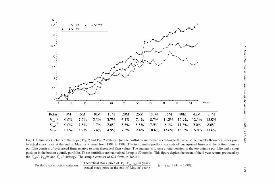
Fig. 3. Future stock returns of the VL1/P, VL2/P, and VL7/P strategy. Quintile portfolios are formed according to the ratio of the model’s theoretical stock price

to actual stock price at the end of May for 8 years from 1991 to 1998. The top quintile portfolio consists of underpriced firms and the bottom quintile

portfolio consists of overpriced firms relative to their theoretical firm values. The strategy is to take a long position in the top quintile portfolio and a short

position in the bottom quintile portfolio. These portfolios are maintained for up to 50 months. This figure depicts the mean of the 8-year returns produced by

the VL1/P, VL2/P, and VL7/P strategy. The sample consists of 674 firms in Table 1.

Portfolio construction criteriont ¼Theoretical stock price of VL1,VL2,VL7 in year t

Actual stock price at the end of May of year tðt ¼ year 1991� 1998Þ:

K.Ota

/TheIntern

atio

nalJournalofAcco

untin

g37(2002)157–182

179

1991 to 1998. The top quintile portfolio consists of underpriced firms and the bottom quintile

portfolio consists of overpriced firms relative to their theoretical firm values. The strategy is

to take a long position in the top quintile portfolio and a short position in the bottom quintile

portfolio, and maintain these positions for up to 50 months.27 Higher future stock returns

indicate better predictive ability of the model. The sample consists of 674 firms selected in

Section 3.2 described earlier.28

Portfolio construction criteriont

¼ Theoretical stock price of VL1,VL2,VL7 in year t

Actual stock price at the end of May of year tðt ¼ year 1991� 1998Þ

VL1/P denotes the abovementioned trading strategy that is based on the VL1 model in Fig. 1.

The VL2/P and the VL7/P strategies are formed in the same manner.

Fig. 3 illustrates the results of the VL1/P, the VL2/P, and the VL7/P strategies. It reveals that

the VL7/P strategy has the greatest ability to predict future stock returns followed by the VL1/P

strategy and the VL2/P strategy. The poor performance of the VL2/P strategy seems to indicate

that the assumption of LIM2, which is that other information nt is a constant, is not

appropriate. The VL7/P strategy earns higher returns than the VL1/P strategy, which appears to

indicate the superiority of LIM7 over LIM1 with respect to the predictive ability of future

stock returns.

Thus, in terms of both explanatory power of contemporaneous stock prices and predictive

ability of future stock returns, the VL7 model performs better than the VL1 model. These

findings support the superiority of LIM7 over LIM1 from the perspective of the stock market

in Japan.

5. Conclusions

This study examines the validity of the Ohlson (1995) information dynamics model and

attempts to improve it. First, the theoretical developments of the RIV and the LIM are

discussed. The LIM is then transformed to give seven empirically testable models, namely,

LIM1–7. These models are tested using a sample of 674 Japanese firms.

LIM1 assumes that abnormal earnings follow a first-order autoregressive process with

other information nt being ignored, and LIM2–6 attempt to improve on this model. The

results of the tests indicate that LIM2–6 basically fail to improve on LIM1. In spite of the

failure, the results of LIM2–6 coupled with those of the Durbin’s alternative test help to

27 The effects of dividends, stock splits, capital reduction, changes in par value, and issuance of new shares on

stock prices are adjusted.28 Actual stock prices are obtained until the end of 1999. Therefore, the portfolios constructed at the end of

May 1996–1998 do not have the complete stock-price data of 50 months. When stock-price data are not available,

the mean returns of the month are calculated without those portfolios.


clarify the empirical problem of testing the Ohlson (1995) LIM. Although other

information, nt, plays an integral role in the Ohlson (1995) LIM, it is often ignored or

assumed wrongly to be a constant because it is unobservable. As a result, other

information, nt, may be absorbed in the error term causing serial correlation in the

errors. This suggests the need for LIM7. Instead of focusing on the difficult problem of

identifying other information, nt, LIM7 tries to circumvent the problem by modeling serial

correlation in the error terms using GLS. LIM7 is a modified version of LIM1, and the

results for LIM7 indicate that LIM7 improves on LIM1 in terms of both Adj. R2 and

Durbin’s alternative statistic.

Moreover, the valuation models of LIM1, LIM2, and LIM7 are derived and they are tested

using Japanese stock market data from two perspectives. The first is the models’ ability to

explain contemporaneous stock prices and the second is the models’ ability to predict future

stock returns. The results from these tests indicate the superiority of the LIM7-based

valuation model over the LIM1-based valuation model.

The findings of this study generally support the validity of the Ohlson (1995) model. They

also indicate that the LIM can be improved by tackling the serially correlated error terms that

may have been caused by the omission of nt.

Acknowledgments

The author gratefully acknowledges the helpful comments and suggestions of Kazuyuki

Suda, Takashi Yaekura, Richard Heaney, A. Rashad Abdel-khalik (editor), anonymous

referees, Atsushi Sasakura, Akinobu Syutou, and Hia Hui Ching.

References

Abarbanell, J., & Bernard, V. (2000). Is the U.S. stock market myopic? Journal of Accounting Research, 38,

221–242.

Akaike, H. (1969). Fitting autoregressive models for prediction. Annals of the Institute of Statistical Mathematics,

21, 243–247.

Akaike, H. (1970). Statistical predictor identification. Annals of the Institute of Statistical Mathematics, 22,

203–217.

Akaike, H. (1973). Information theory and an extension of the maximum likelihood principle. In B. N. Petrov, & F.

Csaki (Eds.), 2nd International Symposium on Information Theory (pp. 267–281). Budapest: Academia Kiado.

Barth, M., Beaver, W., Hand, J., & Landsman, W. (1999). Accruals, cash flows, and equity values. Working paper

(January) (July), Stanford University.

Bar-Yosef, S., Callen, J., & Livnat, J. (1996). Modeling dividends, earnings, and book value equity: an empirical

investigation of the Ohlson valuation dynamics. Review of Accounting Studies, 1, 207–224.

Dechow, P., Hutton, A., & Sloan, R. (1999). An empirical assessment of the residual income valuation model.

Journal of Accounting and Economics, 26, 1–34.

Fama, E., & French, K. (1997). Industry costs of equity. Journal of Accounting and Economics, 43, 153–193.

Feltham, G., & Ohlson, J. (1995). Valuation and clean surplus accounting for operating and financial activities.

Contemporary Accounting Research, 11, 689–731.


Frankel, R., & Lee, C. (1998). Accounting valuation, market expectation, and cross-sectional stock returns.

Journal of Accounting and Economics, 25, 283–319.

Gujarati, D. (1995). Basic econometrics. New York: McGraw-Hill.

Hand, J., & Landsman, W. (1998). Testing the Ohlson model: n or not n that is the question. Working paper,

University of North Carolina.

Hand, J., & Landsman, W. (1999). The pricing of dividends in equity valuation. Working paper, University of

North Carolina.

Hurvich, C., & Tsai, C. (1989). Regression and time series model selection in small samples. Biometrika, 76,

297–307.

Hurvich, C., & Tsai, C. (1991). Bias of the corrected AIC criterion for underfitted regression and time series

model. Biometrika, 78, 499–509.

Johnston, J., & DiNardo, J. (1997). Econometric methods (4th ed.). New York: McGraw-Hill.

Lee, C., Myers, J., & Swaminathan, B. (1999). What is the intrinsic value of the Dow? Journal of Finance, 54,

1693–1741.

Lo, K., & Lys, T. (2000). The Ohlson model: contribution to valuation theory, limitations, and empirical appli-

cations. Journal of Accounting, Auditing and Finance (new series), 15, 337–367.

Lundholm, R. (1995). A tutorial on the Ohlson and Feltham/Ohlson models: answers to some frequently asked

questions. Contemporary Accounting Research, 11, 749–761.

Malkiel, B. (1999). A random walk down Wall Street. New York: W.W. Norton.

Morel, M. (1999). Multi-lagged specification of the Ohlson Model. Journal of Accounting, Auditing and Finance

(new series), 14, 147–161.

Myers, J. (1999). Implementing residual income valuation with linear information dynamics. Accounting Review,

74, 1–28.

O’Hanlon, J. (1994). Clean surplus residual income and earnings based valuation models. Working paper no. 94/

008, Lancaster University.

O’Hanlon, J. (1995). Return/earnings regressions and residual income: empirical evidence. Journal of Business

Finance and Accounting, 22, 53–66.

Ohlson, J. (1995). Earnings, book values and dividends in equity valuation. Contemporary Accounting Research,

11, 661–687.

Palepu, K., Bernard, V., & Healy, P. (1996). Business analysis and valuation. Cincinnati, Ohio, USA: South-

Western College Publishing.

Penman, S., & Sougiannis, T. (1998). A comparison of dividend, cash flow, and earnings approaches to equity

valuation. Contemporary Accounting Research, 15, 343–383.

Qi, D., Wu, Y., & Xiang, B. (2000). Stationarity and cointegration tests of the Ohlson model. Journal of

Accounting, Auditing and Finance (new series), 15, 141–160.


a test of the ohlson (1995) model: empirical evidence from...

Documents