A Theory of Bilateral Oligopoly∗

Kenneth Hendricks

Department of Economics

University of Texas at Austin

Austin TX 78712

R. Preston McAfee

100 Baxter Hall

Humanities & Social Sciences

California Institute of Technology

Pasadena, CA 91125

June 8, 2007

Abstract

In horizontal mergers, concentration is often measured with the Hirschmann-Herfindahl

Index (HHI). This index yields the price-cost margins in Cournot competition. In many

modern merger cases, both buyers and sellers have market power, and indeed, the buy-

ers and sellers may be the same set of firms. In such cases, the HHI is inapplicable.

We develop an alternative theory that has similar data requirements as the HHI, ap-

plies to intermediate good industries with arbitrary numbers of firms on both sides, and

specializes to the HHI when buyers have no market power. The more inelastic is the

downstream demand, the more captive production and consumption (not traded in the

intermediate market) affects price-cost margins. The analysis is applied to the merger

of the gasoline refining and retail assets of Exxon and Mobil in western United States.

∗Acknowledgement: We thank Jeremy Bulow and Paul Klemperer for useful remarks and for encour-aging us to explore downstream concentration.

1

1 Introduction

The seven largest refiners of gasoline on the west coast of the United States account for over

95% of the production of CARB (California Air Resources Board certified) gasoline sold in

the region. The seven largest brands of gasoline also accounts for over 97% of retail sales of

gasoline. Thus, the wholesale gasoline market on the west coast is composed of a number

of large sellers and large buyers who compete against each other in the downstream retail

market. What will be the effect of a merger of vertically integrated firms on the wholesale

and retail markets? This question has relevance with the mergers of Chevron and Texaco,

Conoco and Phillips, Exxon and Mobil, and BP/Amoco and Arco, all of which have been

completed in the past decade.

When monopsony or oligopsony faces an oligopoly, most analysts consider that the need

for protecting buyers from the exercise of market power is mitigated by the market power

of the buyers and vice versa. Thus, even when the buyers and sellers are separate firms,

an analysis based on dispersed buyers or dispersed sellers is likely to err. How should

antitrust authorities account for the power of buyers and sellers in a bilateral oligopoly

market in evaluating the competitiveness of the market? Merging a net buyer with a net

seller produces a more balanced firm, bringing what was formerly traded in the intermediate

good market inside the firm. Will this vertical integration reduce the exercise of market

power and produce a more competitive upstream market? Or will the vertically integrated

firm restrict supply to other non-integrated buyers, particularly if they are rivals in the

downstream market?

There is a voluminous theoretical literature that address these questions. Most of the

literature considers situations in which one or two sellers supply one or two buyers who

compete in a downstream market and models their interactions as a bargaining game.1

Sellers negotiate secret contracts with buyers specifying a quantity to be purchased and

transfers to be paid by the buyer. The bilateral bargaining in these models is efficient,

so there is no distortions in the wholesale market. Gans [12] uses the model of vertical

contracting to derive a concentration index that measures the amount of distortion in the

vertical chain as a result of both horizontal concentration amoung buyers and sellers, and

the degree of vertical integration. However, the vertical contracting models do not describe

1See Rey and Tirole [40] for a survey of this literature. Several of the main papers in this literature areHart and Tirole [21], McAfee and Schwartz [32], O’Brien and Shaffer [38], Segal [43], and de Fontenay andGans [9].

2

intermediate good markets like the wholesale gasoline market in western United States.

The market consists of more than two sellers and two buyers, and trades occur at a fixed,

and observable, price. Other papers study vertical mergers by assigning the market power

either to buyers or to sellers, but not both.2 These models are excellent for assessing

some economic questions, including the incentive to raise rival’s cost, the effects of contact

in several markets, or the consequences of refusals-to-deal. But, they do not address the

implications of bilateral market power that we wish to study in this paper.

Traditional antitrust analysis presumes dispersed buyers. Given such an environment,

the Cournot model (quantity competition) suggests that the Hirschman-Herfindahl Index

(HHI, which is the sum of the squared market shares of the firms) is proportional to the

price-cost margin, which is the proportion of the price that is a markup over marginal cost.

Specifically, the HHI divided by the elasticity of demand equals the price-cost margin. The

HHI is zero for perfect competition and one for monopoly. The HHI has the major advantage

of simplicity and low data requirements. In spite of well-publicized flaws, the HHI continues

to be the workhorse of concentration analysis and is used by both the US Department of

Justice and the Federal Trade Commission. The HHI is inapplicable, however, to markets

where the buyers are concentrated, particularly if they compete in a downstream market.

Our objective in this paper is to offer an alternative to the HHI analysis that applies

to homogenous good markets with linear pricing where buyers are concentrated and with

(i) similar informational requirements, (ii) the Cournot model as a special case, and (iii) an

underlying game as plausible as the Cournot model. The model we offer suffers from the

same flaws as the Cournot model. It is highly stylized and static. It uses a “black box”

pricing mechanism motivated by the Cournot analysis. Moreover, our model will suffer from

the same flaws as the Cournot model in its application to antitrust analysis. Elasticities are

treated as constants when they are not, and the relevant elasticities are taken as known.

However, the analysis can be applied to markets with arbitrary numbers of sellers and

buyers, who individually have the power to influence price, and buyers who may compete

against each other in a downstream market. The analysis is simple to apply, and permits

the calculation of antitrust effects in a practical way.

Our approach is based on the Klemperer and Meyer [23] market game. In their model,

2See for example, Hart and Tirole [21], Ordover, Saloner, and Salop [39], Salinger [41], Salop and Scheff-man [42], Bernheim and Whinston [3]. An alternative to assigning the market power to one side of themarket is Salinger’s sequential model.

3

sellers submit supply functions and behave strategically, buyers are passiveand report their

true demand curves, and price is set to clear the market. We allow the buyers to behave

strategically in submitting their demand functions, and apply a similar concept of equilib-

rium as Klemperer and Meyer. As is well known, supply function models have multiple

equilibria. Klemperer and Meyer [23] reduce the multiplicity by introducing stochastic de-

mand, and they show that, if the support is unbounded, then the equilibrium is unique

and the equilibrium supply schedule is linear. More recently, Holmberg [15][16] has shown

that capacity constraints and a price cap can lead to uniqueness. Green and Newberry [20],

Green [18][19], and Akgun [1] obtain uniqueness by restricting the supply schedules to be

linear. Our approach is similar but we do not require linearity. In our model, sellers can

select from a one-parameter family of schedules indexed by production capacity, and buyers

can select from a one-parameter family of schedules indexed by consumption or retailing

capacity. Thus, sellers can exaggerate their costs by reporting a capacity that is less than it

in fact is, and buyers can understate demand. The main advatage of restricting the selec-

tion of schedules is that it allows us to study the strategic interaction between sellers and

buyers.

In a traditional assessment of concentration according to the U.S. Department of Justice

Merger guidelines, the firms’ market shares are intended, where possible, to be shares of

capacity. This is surprising in light of the fact that the Cournot model does not suggest

the use of capacity shares in the HHI, but rather the share of sales in quantity units (not

revenue). Like the Cournot model, the present study suggests using the sales data, rather

than the capacity data, as the measure of market share. Capacity plays a role in our theory,

and indeed a potential test of the theory is to check that actual capacities, where observed,

are close to the capacities consistent with the theory.

The merger guidelines assess the effect of the merger by summing the market shares of

the merging parties.3 Such a procedure provides a useful approximation but is inconsistent

with the theory (either Cournot or our theory), since the theory suggests that, if the merging

parties’ shares don’t change, then the prices are unlikely to change as well. We advocate

a more computationally-intensive approach, which involves estimating the capacities of the

merging parties from the pre-merger market share data. Given those capacities, we then

estimate the effect of the merger on the industry, taking into account the incentive of the

3Farrell and Shapiro [11] and McAfee and Williams [31] independently criticize the Cournot model whileusing a Cournot model to address the issue.

4

merged firm to restrict output (or demand, in the case of buyers). Horizontal mergers

among sellers in intermediate input market, where buyers are manufacturing firms, are

more likely to raise price and be profitable in our model than in the Cournot model because

capacity reports of sellers are typically strategic complements, not strategic substitutes. In

wholesale markets, the buyers are retailers, and they typically respond to enhanced seller

power by reducing their reported demand, thereby mitigating the effects of the merger

and complicating its impact on prices and profits. The model treats horizontal mergers by

buyers symmetrically. Vertical mergers in our model generate large efficiency gains because

they eliminate two “wedges”, the markup by the seller and the markdown by the buyer.

Foreclosure effects are important when the merging firms are large.

Structural models of homogenous good markets with dispersed buyers use an ad hoc

modification of the Cournot first-order conditions to estimate seller markups. They find

that markups are typically much lower than Cournot markups4 and attribute this finding to

the Cournot model’s failure to account for a firm’s expectations of how rivals will respond

to its output choices. In our model, each firm understands that reductions in its supply

will be partially offset by increases in the outputs of its rivals. Their response means that

the elasticity of each firm’s residual demand function exceeds the elasticity of demand,

so markups are lower in our model than in the Cournot model. Furthemore, the rivals’

responses are determined by their marginal costs, so markups depend upon cost elasticities

as well as the demand elasticity. Larger firms have higher markups, and markups are higher

in markets where marginal costs are steep. Structural models of vertically related markets

typically estimate markups under the assumption that sellers post prices that buyers take

as fixed in a sequential vertical-pricing game.5 In our model, sellers and buyers move

simultaneously and the division of rents from market power depends upon cost and demand

functions.We investigate the conditions under which the first order conditions of our model

can be used to estimate demand and cost parameters.

Our model also provides an interesting alternative for studying spot electricity markets.

The operation of these markets closely resemble our market game: generating firms submit

supply schedules, buyers report the demands of their retail customers who face regulated

prices, and an independent system operator chooses the spot price to equate reported supply

4See Bresnahan [7] for a description of the methodology and a survey of a number of empirical studies.More recent studies include Genesove and Mullin [13] and Clay and Troesken [10]

5Several recent studies include Goldberg and Verboven [17], Manuszak [29], Mortimer [36], Villas-Boas[46], Villas-Boas and Zhao [45], and Villas-Boas and Hellerstein [47].

5

to market demand. Empirical studies of these markets have applied supply function models

or Cournot models to predict the potential for generating firms to exercise market power in

spot electricity markets6 and to estimate their markups7. Our model has the advantages of

the supply function model and the simplicity of the Cournot model.

The second section presents a model of intermediate good markets, derives the equilib-

rium price/cost margins and the value/price margins, which is the equivalent for buyers, for

vertically separated markets and for vertically integrated markets. The third section extends

the model to spot markets in electricity and wholesale markets in which buyers compete in

a downstream market. The fourth section analyzes horizontal and vertical mergers. The

fifth section examines identification issues that would arise in trying to apply our model

to market data. The sixth section applies the model to the merger of the westcoast assets

of Exxon and Mobil to illustrate the plausibility and applicability of the theory. The final

section concludes.

2 Intermediate Good Markets

We begin with a standard model of a market for a homogenous intermediate good Q. There

are n firms, indexed by i from 1 to n. Each seller i produces output xi using a constant

returns to scale production function with fixed capacity γi. Thus, seller i’s production costs

takes the form

C(xi, γi) = γic

µxiγi

¶, (1)

where c(·) is convex and strictly increasing.8 Each buyer j consumes intermediate output qjand values that consumption according to a function V (qj , kj) where kj is buyer j’s capacity

for processing the intermediate output. We assume that V is homogenous of degree one so

6Green and Newbery [20], Green [18], Brunekreeft [8] use supply function models to predict markups inthe England and Wales Wholesale electricity market; Borenstein and Bushnell [5] apply a Cournot model topredict markups in the California electricity markets, and Bushnell, Mansur, and Saravia [4] also use thismodel to predict markups in California, New England, and the Pennsylvania, New Jersey, Maryland (PJM)markets.

7Empirical studies of markups include Borenstein, Bushnell, and Wolak [6] and Wolak [49] on California,Hortacsu and Puller [22] on Texas, Mansur [28] on PJM, Bushnell, Mansur, and Saravia [4] on California,New England, and PJM, Sweeting [44] and Wolfram [52] on England and New Wales, and Wolak [48, 50, 51]on Australia.

8 In addition, we assume that c0(z) −→∞ as z −→∞.

6

that it can expressed as

V (qj , kj) = kjv

µqjkj

¶, (2)

where v(·) is concave and strictly increasing.9 A firm may be both a seller and a buyer,

that is, it may produce the intermediate good and also consume it. Such firms are called

vertically integrated, although they may be net sellers or net buyers. Letting p denote the

market-clearing price in the intermediate good market, the profits to a vertically integrated

firm i are given by

πi = p (xi − qi) + kiv

µqiki

¶− γic

µxiγi

¶. (3)

The profits to a firm if it is either a pure seller or a pure buyer can be obtained by setting

qi = 0 or xi = 0 respectively.

Markets in which both sellers and buyers exercise market power are called bilateral

oligopoly. A market with no vertically integrated firms is called a vertically separated market.

These markets can be further decomposed into oligopoly markets, in which sellers have

market power and buyers do not, and oligopsony markets, in which buyers have market

power but sellers do not. A market with one or more vertically integrated firms is a vertically

integrated market.

In what follows, we will need to distinguish between two kinds of intermediate good

markets based on the type of buyer. Markets in which buyers are manufacturing firms are

called intermediate input markets. In these markets, a buyer j combines the intermediate

input qj with capacity kj using a constant returns to scale technology F (qj , kj) to produce

a good yj that it sells at price r.10 Thus, its revenue function can be expressed as

V (qj , kj) = rkif

µqiki

¶A manufacturing firm that has twice the capacity of another firm can produce twice as

much at the same average productivity.

Markets in which buyers are retail firms are called wholesale markets. In these markets,

a buyer j purchases qj to resell to final consumers at price r. Here yj = qj and firm j’s

9 In addition, we assume v0(z) −→ 0 as z −→∞.10The production function could include other inputs provided their quantities are proportional to qi.

7

valuation of qj is given by

V (qj , kj) = rqj − kjw

µqjkj

¶= kj

∙r

µqjkj

¶− w

µqjkj

¶¸where w represents unit selling costs. A retailer with twice as much selling capacity (e.g.,

number of stores) can sell twice as much at the same unit cost.

In the Cournot model of oligopoly markets, sellers submit quantities and the market

chooses price to equate reported supply to demand. The equilibrium price is equal to each

buyer’s marginal willingness-to-pay but exceeds each seller’s marginal cost of supply. In the

standard oligopsony model, buyers submit quantities and the market chooses price to equate

reported supply and demand. The equilibrium price is equal to each seller’s marginal cost

but exceeds each buyer’s true willingness to pay. In each of these models, one side of the

market is passive and the other side behaves strategically, anticipating the market-clearing

mechanism in order to manipulate prices. Our interest, however, is in a market where

both buyers and sellers recognize their ability to unilaterally influence the price and behave

strategically. In order to model this type of market, we extend the Klemperer and Meyer

model, in which sellers behave strategically in submitting supply schedules, to allow buyers

to behave strategically in submitting their demand schedules.

In adopting this model, however, we impose some restrictions on the schedules that the

firms can report. Sellers have to submit cost schedules which come in the form γc(x/γ), and

buyers have to submit valuation functions which come in the form kv(q/k). In a mechanism

design framework, agents can lie about their type, but they cannot invent an impossible

type. The admissible types in our model satisfy (1) and (2), and agents are assumed to

be bound by this message space. For sellers, the message space is a one-parameter family

of schedules indexed by production capacity, and for buyers, the message space is a one-

parameter family of schedules indexed by consumption capacity. Therefore, a seller’s type

is a capacity γ, a buyer’s type is a capacity k,and if the firm is vertically integrated, its

type is a pair of capacities (γ, k). Agents (simultaneously) report their types to the market

mechanism but, in doing so, they do not have to tell the truth. A seller can exaggerate its

costs by reporting a capacity bγ that is less than it in fact is, and a buyer can understateits willingness to pay by reporting a capacity bk that is less than it in fact is.11 Values and11A buyer’s marginal willingness to pay for another unit of input at q units of input is measured by v0

¡qk

¢.

Since v is concave, this derivative is increasing in k. Therefore, a buyer understates its willingness to pay

8

costs are not well-specified at zero capacity. However, the solution can be calculated for

arbitrarily small but positive capacities and zero capacity handled as a limit. Firms with

zero capacity would then report zero capacity.

Given the agents’ reports, the market mechanism chooses price p to equate reported sup-

ply and reported demand, and allocates the output efficiently. The solution is characterized

by the balance equation,

Q =nXi=1

qi =nXi=1

xi = X (4)

and the marginal conditions,

v0Ãqjbkj!= p = c0

µxibγi¶, i, j = 1, .., n. (5)

Note that, if everyone tells the truth, then the equilibrium outcome is efficient. Our model

can be viewed as turning the market into a black box, as in fact happens in the Cournot

model, where the price formation process is not modeled explicitly. Given this black box

approach, it seems appropriate to permit the market to be efficient when agents don’t,

in fact, exercise unilateral power. Such considerations dictate the competitive solution,

given the reported types. Any other assumption would impose inefficiencies in the market

mechanism, rather than having inefficiencies arise as the consequence of the rational exercise

of market power by firms with significant market presence.

Each firm anticipates the market mechanism’s decision rule in submitting its reports.

From equation (4), it follows that

qi =bkiQK

, xi =bγiQΓ

, (6)

where

K =nXi=1

bki, Γ = nXi=1

bγi. (7)

Thus, given the firms’ reports, market output Q(Γ,K) solves the equation

v0µQ

K

¶= c0

µQ

Γ

¶, (8)

by underreporting its capacity.

9

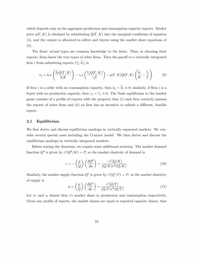
which depends only on the aggregate production and consumption capacity reports. Market

price p(Γ,K) is obtained by substituting Q(Γ,K) into the marginal conditions of equation

(4), and the output is allocated to sellers and buyers using the market share equations of

(5).

The firms’ actual types are common knowledge to the firms. Thus, in choosing their

reports, firms know the true types of other firms. Then the payoff to a vertically integrated

firm i from submitting reports (bγi,bki) isπi = kiv

ÃbkiQ(Γ,K)kiK

!− γic

µbγiQ(Γ,K)γiΓ

¶− p(Γ,K)Q(Γ,K)

ÃbkiK− bγiΓ

!. (9)

If firm i is a seller with no consumption capacity, then ki = bki ≡ 0; similarly, if firm i is a

buyer with no production capacity, then γi = bγi ≡ 0. The Nash equilibrium to the market

game consists of a profile of reports with the property that (i) each firm correctly guesses

the reports of other firms and (ii) no firm has an incentive to submit a different, feasible

report.

2.1 Equilibrium

We first derive and discuss equilibrium markups in vertically separated markets. We con-

sider several special cases including the Cournot model. We then derive and discuss the

equilibrium markups in vertically integrated markets.

Before stating the theorems, we require some additional notation. The market demand

function Qd is given by v0(Qd/K) = P, so the market elasticity of demand is

ε = −µp

Q

¶µdQd

dp

¶=

−v0(Q/K)(Q/K)v00(Q/K)

. (10)

Similarly, the market supply function Qs is given by c0(Qs/Γ) = P , so the market elasticity

of supply is

η =

µp

Q

¶µdQs

dp

¶=

c0(Q/Γ)

(Q/Γ)c00(Q/Γ). (11)

Let σi and si denote firm i’s market share in production and consumption respectively.

Given any profile of reports, the market shares are equal to reported capacity shares, that

10

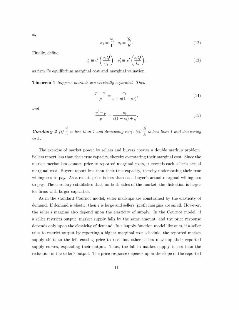
is,

σi =bγiΓ, si =

bkiK. (12)

Finally, define

c0i ≡ c0µσiQ

γi

¶, v0i ≡ v0

µsiQ

ki

¶. (13)

as firm i’s equilibrium marginal cost and marginal valuation.

Theorem 1 Suppose markets are vertically separated. Then

p− c0ip

=σi

ε+ η(1− σi), (14)

andv0i − p

p=

siε(1− si) + η

. (15)

Corollary 2 (i)bγγis less than 1 and decreasing in γ; (ii)

bkkis less than 1 and decreasing

in k.

The exercise of market power by sellers and buyers creates a double markup problem.

Sellers report less than their true capacity, thereby overstating their marginal cost. Since the

market mechanism equates price to reported marginal costs, it exceeds each seller’s actual

marginal cost. Buyers report less than their true capacity, thereby understating their true

willingness to pay. As a result, price is less than each buyer’s actual marginal willingness

to pay. The corollary establishes that, on both sides of the market, the distortion is larger

for firms with larger capacities.

As in the standard Cournot model, seller markups are constrained by the elasticity of

demand. If demand is elastic, then ε is large and sellers’ profit margins are small. However,

the seller’s margins also depend upon the elasticity of supply. In the Cournot model, if

a seller restricts output, market supply falls by the same amount, and the price response

depends only upon the elasticity of demand. In a supply function model like ours, if a seller

tries to restrict output by reporting a higher marginal cost schedule, the reported market

supply shifts to the left causing price to rise, but other sellers move up their reported

supply curves, expanding their output. Thus, the fall in market supply is less than the

reduction in the seller’s output. The price response depends upon the slope of the reported

11

supply curves. If marginal costs are roughly constant (i.e., c00 ' 0), then η is very large,

individual sellers cannot raise price significantly by constricting their supply schedule, and

the Bertrand outcome arises. On the other hand, if marginal cost curves are steeply sloped

(i.e., c00/c0 −→∞), then η approaches 0, and the Cournot outcome arises. Since our model

treats buyers and sellers symmetrically, the same reasoning applies to buyer markups.

We turn next to vertically integrated markets.

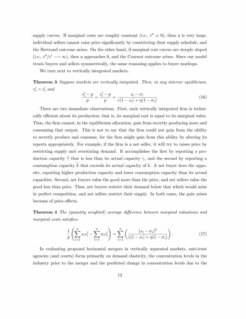
Theorem 3 Suppose markets are vertically integrated. Then, in any interior equilibrium,

v0i = c0i andv0i − p

p=

c0i − p

p=

si − σiε(1− si) + η(1− σi)

. (16)

There are two immediate observations. First, each vertically integrated firm is techni-

cally efficient about its production; that is, its marginal cost is equal to its marginal value.

Thus, the firm cannot, in the equilibrium allocation, gain from secretly producing more and

consuming that output. This is not to say that the firm could not gain from the ability

to secretly produce and consume, for the firm might gain from this ability by altering its

reports appropriately. For example, if the firm is a net seller, it will try to raises price by

restricting supply and overstating demand. It accomplishes the first by reporting a pro-

duction capacity bγ that is less than its actual capacity γ, and the second by reporting a

consumption capacity bk that exceeds its actual capacity of k. A net buyer does the oppo-site, reporting higher production capacity and lower consumption capacity than its actual

capacities. Second, net buyers value the good more than the price, and net sellers value the

good less than price. Thus, net buyers restrict their demand below that which would arise

in perfect competition, and net sellers restrict their supply. In both cases, the gain arises

because of price effects.

Theorem 4 The (quantity weighted) average difference between marginal valuations and

marginal costs satisfies:

1

p

ÃnXi=1

siv0i −

nXi=1

σic0i

!=

nXi=1

µ(si − σi)

2

ε(1− si) + η(1− σi)

¶. (17)

In evaluating proposed horizontal mergers in vertically separated markets, anti-trust

agencies (and courts) focus primarily on demand elasticity, the concentration levels in the

industry prior to the merger and the predicted change in concentration levels due to the

12

merger, where concentration is measured using the Herfindahl-Hirschman index. This analy-

sis is motivated by the Cournot model. Theorem 4 gives the equivalent of the Hirschman-

Herfindahl Index (H) for the present model. We will refer to it as the modified Hirschman-

herfindahl Index (MHI). It has the same useful features — it depends only on market

shares and elasticities — but there are two important differences. First, it suggests that

analysts also need to consider the elasticity of supply in evaluating the competitiveness of

the market. Second, it generalizes the analysis to vertically integrated markets and suggests

that analysts use the firms’ net positions to measure the effects of market power. As noted

above, zero net demand causes no inefficiency. Thus, an intermediate good market in which

each firm is vertically integrated and supplies only itself is perfectly efficient. However, with

even a small but nonzero net demand or supply, size exacerbates the inefficiency.

In this framework, the shares are of production or consumption, and not capacity. The

U.S. Department of Justice Merger Guidelines [53] generally calls for evaluation shares of

capacity. While our analysis begins with capacities, the shares are actual shares of produc-

tion (σi) or consumption (si), rather than the capacity for production and consumption,

respectively. Firms may have the same capacity in production and consumption but nev-

ertheless choose to be a net seller or a net buyer depending upon market conditions. The

use of actual consumption and production is an advantageous feature of the theory, since

these values tend to be readily observed, while capacities are not. Moreover, capacity is

often subject to vociferous debate by economic analysts, while the market shares may be

more readily observable. Finally, the shares are shares of the total quantity and not revenue

shares. However, like the Cournot model, our model is not designed to handle industries

with differentiated products, which is the situation where a debate about revenue versus

quantity shares arises.

2.2 Intermediate Input Markets with Constant Elasticities

An important special case of our model is one in which value and cost elasticities are

constant and buyers are manufacturing firms. Suppose marginal cost is given by

c0(z) = az1η ,

13

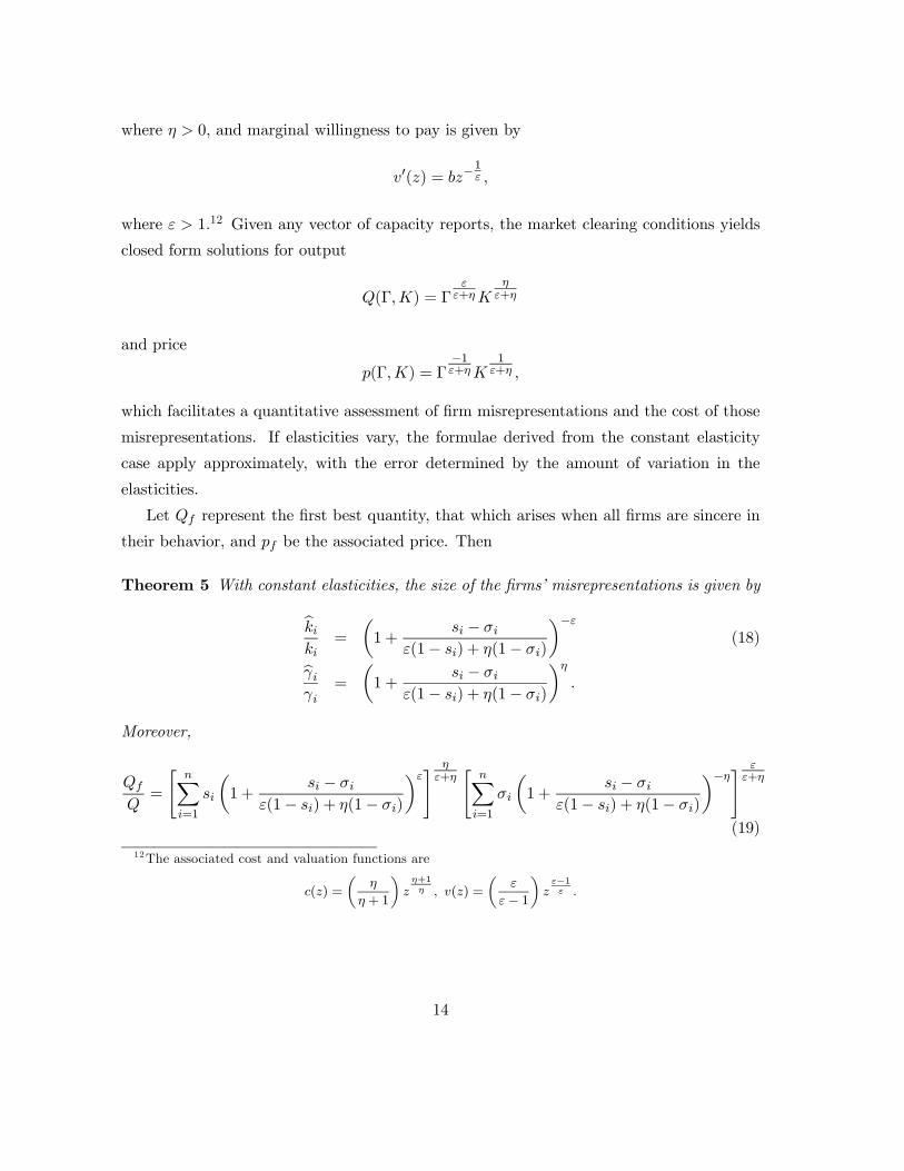
where η > 0, and marginal willingness to pay is given by

v0(z) = bz−1ε ,

where ε > 1.12 Given any vector of capacity reports, the market clearing conditions yields

closed form solutions for output

Q(Γ,K) = Γε

ε+ηKη

ε+η

and price

p(Γ,K) = Γ−1ε+ηK

1ε+η ,

which facilitates a quantitative assessment of firm misrepresentations and the cost of those

misrepresentations. If elasticities vary, the formulae derived from the constant elasticity

case apply approximately, with the error determined by the amount of variation in the

elasticities.

Let Qf represent the first best quantity, that which arises when all firms are sincere in

their behavior, and pf be the associated price. Then

Theorem 5 With constant elasticities, the size of the firms’ misrepresentations is given by

bkiki

=

µ1 +

si − σiε(1− si) + η(1− σi)

¶−ε(18)

bγiγi

=

µ1 +

si − σiε(1− si) + η(1− σi)

¶η

.

Moreover,

Qf

Q=

"nXi=1

si

µ1 +

si − σiε(1− si) + η(1− σi)

¶ε# ηε+η

"nXi=1

σi

µ1 +

si − σiε(1− si) + η(1− σi)

¶−η# εε+η

(19)

12The associated cost and valuation functions are

c(z) =

µη

η + 1

¶zη+1η , v(z) =

µε

ε− 1

¶zε−1ε .

14

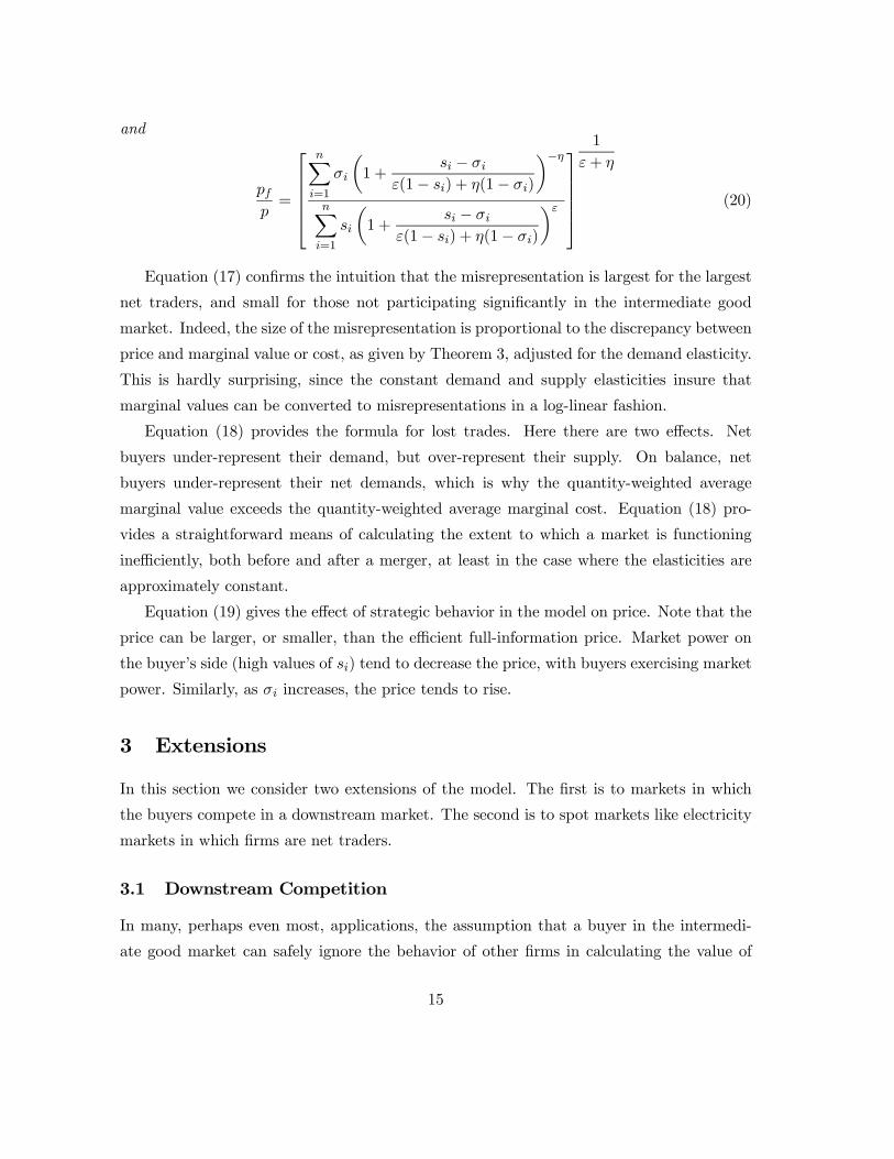
and

pfp=

⎡⎢⎢⎢⎢⎣nXi=1

σi

µ1 +

si − σiε(1− si) + η(1− σi)

¶−ηnXi=1

si

µ1 +

si − σiε(1− si) + η(1− σi)

¶ε

⎤⎥⎥⎥⎥⎦

1

ε+ η

(20)

Equation (17) confirms the intuition that the misrepresentation is largest for the largest

net traders, and small for those not participating significantly in the intermediate good

market. Indeed, the size of the misrepresentation is proportional to the discrepancy between

price and marginal value or cost, as given by Theorem 3, adjusted for the demand elasticity.

This is hardly surprising, since the constant demand and supply elasticities insure that

marginal values can be converted to misrepresentations in a log-linear fashion.

Equation (18) provides the formula for lost trades. Here there are two effects. Net

buyers under-represent their demand, but over-represent their supply. On balance, net

buyers under-represent their net demands, which is why the quantity-weighted average

marginal value exceeds the quantity-weighted average marginal cost. Equation (18) pro-

vides a straightforward means of calculating the extent to which a market is functioning

inefficiently, both before and after a merger, at least in the case where the elasticities are

approximately constant.

Equation (19) gives the effect of strategic behavior in the model on price. Note that the

price can be larger, or smaller, than the efficient full-information price. Market power on

the buyer’s side (high values of si) tend to decrease the price, with buyers exercising market

power. Similarly, as σi increases, the price tends to rise.

3 Extensions

In this section we consider two extensions of the model. The first is to markets in which

the buyers compete in a downstream market. The second is to spot markets like electricity

markets in which firms are net traders.

3.1 Downstream Competition

In many, perhaps even most, applications, the assumption that a buyer in the intermedi-

ate good market can safely ignore the behavior of other firms in calculating the value of

15

consumption is unfounded. This is particularly true when the buyers are retail firms. In

this section, we extend the model to wholesale markets in which retail firms compete in

quantities in the downstream market.

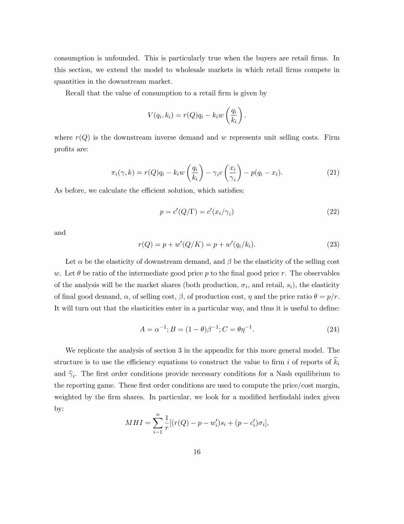
Recall that the value of consumption to a retail firm is given by

V (qi, ki) = r(Q)qi − kiw

µqiki

¶.

where r(Q) is the downstream inverse demand and w represents unit selling costs. Firm

profits are:

πi(γ, k) = r(Q)qi − kiw

µqiki

¶− γic

µxiγi

¶− p(qi − xi). (21)

As before, we calculate the efficient solution, which satisfies:

p = c0(Q/Γ) = c0(xi/γi) (22)

and

r(Q) = p+ w0(Q/K) = p+w0(qi/ki). (23)

Let α be the elasticity of downstream demand, and β be the elasticity of the selling cost

w. Let θ be ratio of the intermediate good price p to the final good price r. The observables

of the analysis will be the market shares (both production, σi, and retail, si), the elasticity

of final good demand, α, of selling cost, β, of production cost, η and the price ratio θ = p/r.

It will turn out that the elasticities enter in a particular way, and thus it is useful to define:

A = α−1;B = (1− θ)β−1;C = θη−1. (24)

We replicate the analysis of section 3 in the appendix for this more general model. The

structure is to use the efficiency equations to construct the value to firm i of reports of bkiand bγi. The first order conditions provide necessary conditions for a Nash equilibrium to

the reporting game. These first order conditions are used to compute the price/cost margin,

weighted by the firm shares. In particular, we look for a modified herfindahl index given

by:

MHI =nXi−1

1

r[(r(Q)− p−w0i)si + (p− c0i)σi],

16

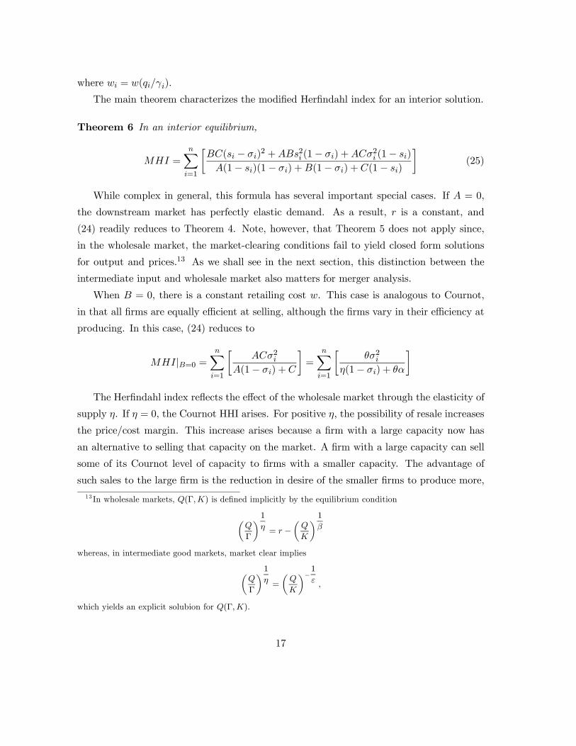
where wi = w(qi/γi).

The main theorem characterizes the modified Herfindahl index for an interior solution.

Theorem 6 In an interior equilibrium,

MHI =nXi=1

∙BC(si − σi)

2 +ABs2i (1− σi) +ACσ2i (1− si)

A(1− si)(1− σi) +B(1− σi) + C(1− si)

¸(25)

While complex in general, this formula has several important special cases. If A = 0,

the downstream market has perfectly elastic demand. As a result, r is a constant, and

(24) readily reduces to Theorem 4. Note, however, that Theorem 5 does not apply since,

in the wholesale market, the market-clearing conditions fail to yield closed form solutions

for output and prices.13 As we shall see in the next section, this distinction between the

intermediate input and wholesale market also matters for merger analysis.

When B = 0, there is a constant retailing cost w. This case is analogous to Cournot,

in that all firms are equally efficient at selling, although the firms vary in their efficiency at

producing. In this case, (24) reduces to

MHI|B=0 =nXi=1

∙ACσ2i

A(1− σi) + C

¸=

nXi=1

∙θσ2i

η(1− σi) + θα

¸

The Herfindahl index reflects the effect of the wholesale market through the elasticity of

supply η. If η = 0, the Cournot HHI arises. For positive η, the possibility of resale increases

the price/cost margin. This increase arises because a firm with a large capacity now has

an alternative to selling that capacity on the market. A firm with a large capacity can sell

some of its Cournot level of capacity to firms with a smaller capacity. The advantage of

such sales to the large firm is the reduction in desire of the smaller firms to produce more,

13 In wholesale markets, Q(Γ,K) is defined implicitly by the equilibrium condition

µQ

Γ

¶ 1η = r −

µQ

K

¶ 1β

whereas, in intermediate good markets, market clear implies

µQ

Γ

¶ 1η =

µQ

K

¶−1ε ,

which yields an explicit solubion for Q(Γ,K).

17

which helps increase the retail price. In essence, the larger firms buy off the smaller firms

via sales in the intermediate good market, thereby reducing the incentive of the smaller

firms to increase their production.

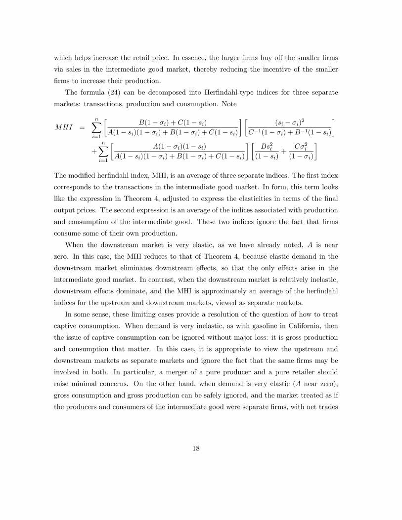
The formula (24) can be decomposed into Herfindahl-type indices for three separate

markets: transactions, production and consumption. Note

MHI =nXi=1

∙B(1− σi) + C(1− si)

A(1− si)(1− σi) +B(1− σi) + C(1− si)

¸ ∙(si − σi)

2

C−1(1− σi) +B−1(1− si)

¸

+nXi=1

∙A(1− σi)(1− si)

A(1− si)(1− σi) +B(1− σi) + C(1− si)

¸ ∙Bs2i

(1− si)+

Cσ2i(1− σi)

¸

The modified herfindahl index, MHI, is an average of three separate indices. The first index

corresponds to the transactions in the intermediate good market. In form, this term looks

like the expression in Theorem 4, adjusted to express the elasticities in terms of the final

output prices. The second expression is an average of the indices associated with production

and consumption of the intermediate good. These two indices ignore the fact that firms

consume some of their own production.

When the downstream market is very elastic, as we have already noted, A is near

zero. In this case, the MHI reduces to that of Theorem 4, because elastic demand in the

downstream market eliminates downstream effects, so that the only effects arise in the

intermediate good market. In contrast, when the downstream market is relatively inelastic,

downstream effects dominate, and the MHI is approximately an average of the herfindahl

indices for the upstream and downstream markets, viewed as separate markets.

In some sense, these limiting cases provide a resolution of the question of how to treat

captive consumption. When demand is very inelastic, as with gasoline in California, then

the issue of captive consumption can be ignored without major loss: it is gross production

and consumption that matter. In this case, it is appropriate to view the upstream and

downstream markets as separate markets and ignore the fact that the same firms may be

involved in both. In particular, a merger of a pure producer and a pure retailer should

raise minimal concerns. On the other hand, when demand is very elastic (A near zero),

gross consumption and gross production can be safely ignored, and the market treated as if

the producers and consumers of the intermediate good were separate firms, with net trades

18

in the intermediate good the only issue that arises.14 Few real world cases are likely to

approximate the description of very elastic market demand.15 However, the case of A = 0

also corresponds to the case where the buyers do not compete in a downstream market, and

thus may have alternative applications.

In the appendix, we provide the formulae governing the special case of constant elas-

ticities. It is straightforward to compute the reduction in quantity that arises from a

concentrated market, as a proportion of the fully efficient, first-best quantity. Moreover, we

provide programs which takes market shares as inputs and computes the capital shares of

the firms, the quantity reduction and the effects of a merger.16

3.2 Electricity Markets

In day-ahead or real-time balancing markets, generating firms submit supply schedules,

buyers report the amounts that they need for their retail customers, and an independent

system operator chooses price to equate reported supply to market demand. Thus, our

market game closely approximates the way in which these markets operate. An important

factor determining the generating firms bidding behavior in these markets is their contract

positions. With the exception of firms in the California market, generating firms typically

sign forward contracts with buyers in which they agree to deliver a fixed amount of electricity

at a pre-determined price. Generating firms who have signed such vertical contracts are

essentially vertically integrated, and they may be net sellers or net buyers in the spot

market. Green [19] and Wolak [48] discuss the theoretical implications of forward contracts

and show that they make the spot market more competitive.

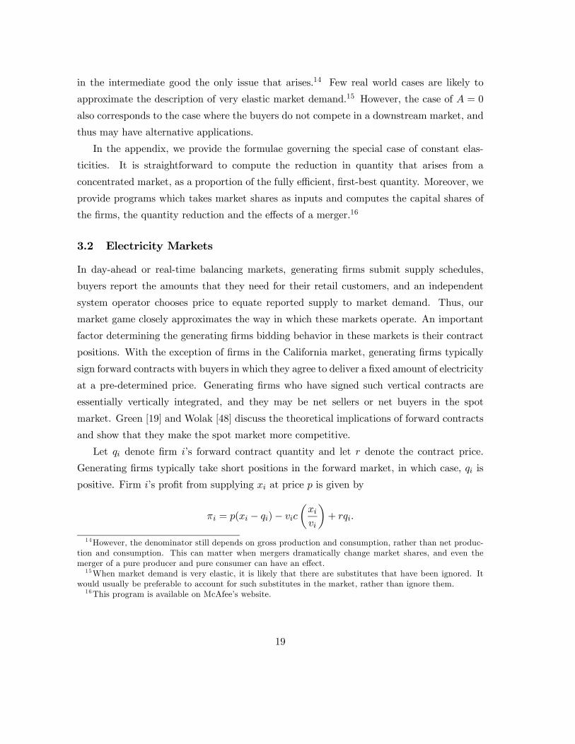
Let qi denote firm i’s forward contract quantity and let r denote the contract price.

Generating firms typically take short positions in the forward market, in which case, qi is

positive. Firm i’s profit from supplying xi at price p is given by

πi = p(xi − qi)− vic

µxivi

¶+ rqi.

14However, the denominator still depends on gross production and consumption, rather than net produc-tion and consumption. This can matter when mergers dramatically change market shares, and even themerger of a pure producer and pure consumer can have an effect.15When market demand is very elastic, it is likely that there are substitutes that have been ignored. It

would usually be preferable to account for such substitutes in the market, rather than ignore them.16This program is available on McAfee’s website.

19

The firm’s revenues consists of two components: the amount it earns from its contract posi-

tion and the payment it receives from either reducing its supply below qi or from increasing

its supply above qi. When it reduces its supply, it is in a net buyer position, buying the

reduction in supply at price p from the spot market and selling this amount to its customers

at the contract price of r. When it increases its supply, firm i is in a net seller position,

selling the increase at price p to retailers. The profit function can also be interpreted as

the profits of a vertically integrated firm that sells electricity to its retail customers at a

regulated price of r.

We assume that the firms face a downward sloping inverse demand function p(X)17

The operator knows the marginal cost schedules but does not know the capacity that firms

have available or at least cannot force them to make all of their capacity available. Firms

are asked to report their available generating capacities. Contract positions are common

knowledge among the firms. Based on these reports, the operator equates demand to supply

and allocates output across firms by equating reported marginal costs so in equilibrium,

p(X) = c0³xibν ´

and for i = 1, .., n. Note that the allocation rule does not depend upon the firms’ contract

positions so firms only report their production capacity. Let α(p) is the elasticity of demand

at price p and define si = qi/X.

Theorem 7 In an interior equilibrium

p− c0ip

=σi − si

η(1− σi) + α.

The theorem states that the firm’s reported capacity exceeds its true capacity (i.e.,

marginal cost exceeds reported marginal cost) when the firm produces less than its contract

quantity and the opposite is true when it produces more than its contract quantity. It

reports truthfully when it is balanced. (If demand is perfectly inelastic, then α is equal to

zero in the above formula.) The intuition is that, in former case, the firm is in a net buy

position and wants to lower price, whereas in the latter case, it is in a net sell position and

wants to raise price. Markups in our model will vary across firms depending upon their

17Market demand is downward-sloping in some electricity markets because it is equal to the fixed retaildemand less a competitive import supply.

20

contract positions, and with demand conditions if the elasticity of costs is not constant.

Since marginal cost functions in the electricity markets are approximately L-shaped, our

model predicts that markups are essentially zero in low demand periods and higher during

high demand periods, particularly for large net sellers. This is consistent with the evidence

presented in Bushnell, Mansur, and Saravia (BMS) [4].18 They find that prices are very

close to marginal costs during off-peak hours and higher during peak hours.

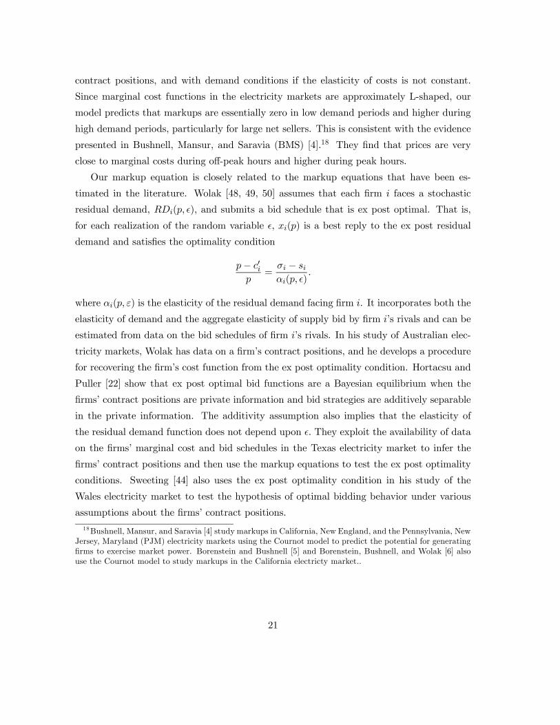
Our markup equation is closely related to the markup equations that have been es-

timated in the literature. Wolak [48, 49, 50] assumes that each firm i faces a stochastic

residual demand, RDi(p, ), and submits a bid schedule that is ex post optimal. That is,

for each realization of the random variable , xi(p) is a best reply to the ex post residual

demand and satisfies the optimality condition

p− c0ip

=σi − siαi(p, )

.

where αi(p, ε) is the elasticity of the residual demand facing firm i. It incorporates both the

elasticity of demand and the aggregate elasticity of supply bid by firm i’s rivals and can be

estimated from data on the bid schedules of firm i’s rivals. In his study of Australian elec-

tricity markets, Wolak has data on a firm’s contract positions, and he develops a procedure

for recovering the firm’s cost function from the ex post optimality condition. Hortacsu and

Puller [22] show that ex post optimal bid functions are a Bayesian equilibrium when the

firms’ contract positions are private information and bid strategies are additively separable

in the private information. The additivity assumption also implies that the elasticity of

the residual demand function does not depend upon . They exploit the availability of data

on the firms’ marginal cost and bid schedules in the Texas electricity market to infer the

firms’ contract positions and then use the markup equations to test the ex post optimality

conditions. Sweeting [44] also uses the ex post optimality condition in his study of the

Wales electricity market to test the hypothesis of optimal bidding behavior under various

assumptions about the firms’ contract positions.

18Bushnell, Mansur, and Saravia [4] study markups in California, New England, and the Pennsylvania, NewJersey, Maryland (PJM) electricity markets using the Cournot model to predict the potential for generatingfirms to exercise market power. Borenstein and Bushnell [5] and Borenstein, Bushnell, and Wolak [6] alsouse the Cournot model to study markups in the California electricty market..

21

4 Mergers

In this section we examine the equilibrium effects of horizontal and vertical mergers. The

constant returns to scale assumption facilitates the study of mergers. It implies that the

merger of two firms i and j produces a firm with consumption capacity ki+ kj and produc-

tion capacity γi+γj , and thereby is subject to the same analysis. In what follows, we focus

primarily on mergers in vertically separated markets for two reasons. First, previous merger

studies typically make this assumption and we wish to compare the results of our analysis

to their results. Second, the vertically separated market provides a polar case in which qual-

itative results can be obtained under the assumption of constant elasticities. The analysis

illustrates the economic forces at work in vertically integrated markets, where the impact

of mergers depends upon the values of the elasticity parameters and hence requires a more

quantitative analysis. We will assume throughout this section that elasticities, including

that of downstream demand, are constant.

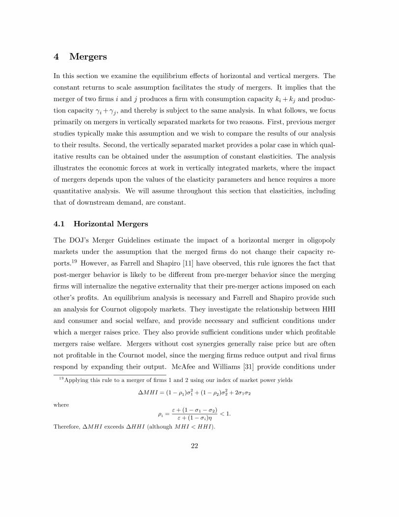
4.1 Horizontal Mergers

The DOJ’s Merger Guidelines estimate the impact of a horizontal merger in oligopoly

markets under the assumption that the merged firms do not change their capacity re-

ports.19 However, as Farrell and Shapiro [11] have observed, this rule ignores the fact that

post-merger behavior is likely to be different from pre-merger behavior since the merging

firms will internalize the negative externality that their pre-merger actions imposed on each

other’s profits. An equilibrium analysis is necessary and Farrell and Shapiro provide such

an analysis for Cournot oligopoly markets. They investigate the relationship between HHI

and consumer and social welfare, and provide necessary and sufficient conditions under

which a merger raises price. They also provide sufficient conditions under which profitable

mergers raise welfare. Mergers without cost synergies generally raise price but are often

not profitable in the Cournot model, since the merging firms reduce output and rival firms

respond by expanding their output. McAfee and Williams [31] provide conditions under

19Applying this rule to a merger of firms 1 and 2 using our index of market power yields

∆MHI = (1− ρ1)σ21 + (1− ρ2)σ

22 + 2σ1σ2

where

ρi =ε+ (1− σ1 − σ2)

ε+ (1− σi)η< 1.

Therefore, ∆MHI exceeds ∆HHI (although MHI < HHI).

22

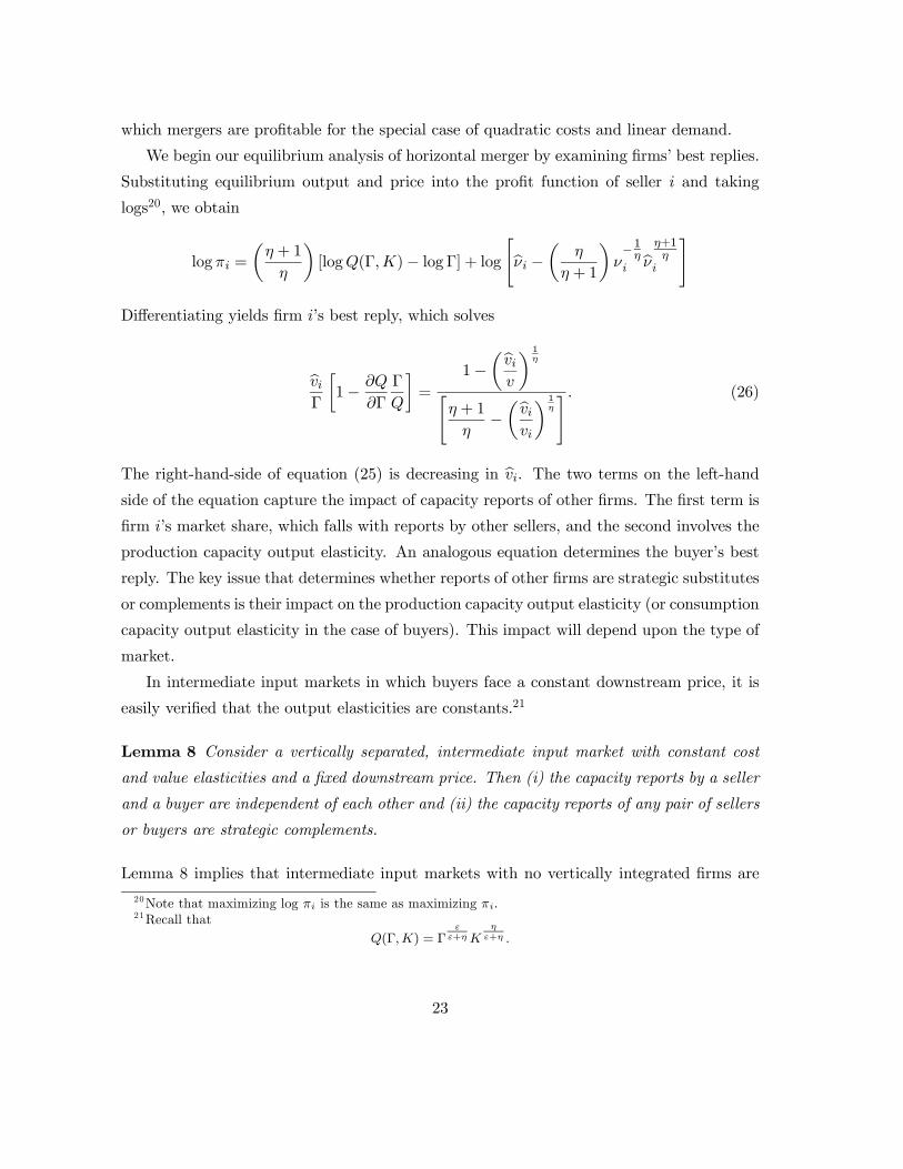
which mergers are profitable for the special case of quadratic costs and linear demand.

We begin our equilibrium analysis of horizontal merger by examining firms’ best replies.

Substituting equilibrium output and price into the profit function of seller i and taking

logs20, we obtain

log πi =

µη + 1

η

¶[logQ(Γ,K)− logΓ] + log

"bνi −µ η

η + 1

¶ν−1ηi bν η+1

ηi

#

Differentiating yields firm i’s best reply, which solves

bviΓ

∙1− ∂Q

∂Γ

Γ

Q

¸=

1−µbviv

¶ 1η

"η + 1

η−µbvivi

¶ 1η

# . (26)

The right-hand-side of equation (25) is decreasing in bvi. The two terms on the left-handside of the equation capture the impact of capacity reports of other firms. The first term is

firm i’s market share, which falls with reports by other sellers, and the second involves the

production capacity output elasticity. An analogous equation determines the buyer’s best

reply. The key issue that determines whether reports of other firms are strategic substitutes

or complements is their impact on the production capacity output elasticity (or consumption

capacity output elasticity in the case of buyers). This impact will depend upon the type of

market.

In intermediate input markets in which buyers face a constant downstream price, it is

easily verified that the output elasticities are constants.21

Lemma 8 Consider a vertically separated, intermediate input market with constant cost

and value elasticities and a fixed downstream price. Then (i) the capacity reports by a seller

and a buyer are independent of each other and (ii) the capacity reports of any pair of sellers

or buyers are strategic complements.

Lemma 8 implies that intermediate input markets with no vertically integrated firms are

20Note that maximizing log πi is the same as maximizing πi.21Recall that

Q(Γ,K) = Γε

ε+ηKη

ε+η .

23

not only structurally separate, they are also strategically separate. It also implies that the

reporting game is a log supermodular game.22

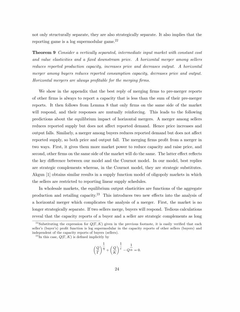
Theorem 9 Consider a vertically separated, intermediate input market with constant cost

and value elasticities and a fixed downstream price. A horizontal merger among sellers

reduces reported production capacity, increases price and decreases output. A horizontal

merger among buyers reduces reported consumption capacity, decreases price and output.

Horizontal mergers are always profitable for the merging firms.

We show in the appendix that the best reply of merging firms to pre-merger reports

of other firms is always to report a capacity that is less than the sum of their pre-merger

reports. It then follows from Lemma 8 that only firms on the same side of the market

will respond, and their responses are mutually reinforcing. This leads to the following

predictions about the equilibrium impact of horizontal mergers. A merger among sellers

reduces reported supply but does not affect reported demand. Hence price increases and

output falls. Similarly, a merger among buyers reduces reported demand but does not affect

reported supply, so both price and output fall. The merging firms profit from a merger in

two ways. First, it gives them more market power to reduce capacity and raise price, and

second, other firms on the same side of the market will do the same. The latter effect reflects

the key difference between our model and the Cournot model. In our model, best replies

are strategic complements whereas, in the Cournot model, they are strategic substitutes.

Akgun [1] obtains similar results in a supply function model of oligopoly markets in which

the sellers are restricted to reporting linear supply schedules.

In wholesale markets, the equilibrium output elasticities are functions of the aggregate

production and retailing capacity.23 This introduces two new effects into the analysis of

a horizontal merger which complicates the analysis of a merger. First, the market is no

longer strategically separate. If two sellers merge, buyers will respond. Tedious calculations

reveal that the capacity reports of a buyer and a seller are strategic complements as long22Substituting the expression for Q(Γ,K) given in the previous footnote, it is easily verified that each

seller’s (buyer’s) profit function is log supermodular in the capacity reports of other sellers (buyers) andindependent of the capacity reports of buyers (sellers).23 In this case, Q(Γ,K) is defined implicitly by

µQ

Γ

¶ 1η +

µQ

K

¶1ε −Q

1

α = 0.

24

as downstream demand is not too inelastic.24 Thus, when the merging sellers try to reduce

their reported capacity, buyers will reduce their capacity reports, thereby lowering reported

demand. In this way, the enhanced market power of sellers is mitigated by buyers exercising

buyer power. Prices are lower, mergers are less profitable, and inefficiency costs increase.

In fact, the strategic complementarity between the buyer and seller reports can lead to

nonexistence of an interior solution. For example, if the merger among sellers creates a

monopoly, and there is only one buyer who sells at a fixed price of r, it can be shown

that the only intersection point of the best replies is (0,0). Clearly, in this case, a merger

would not be profitable. Second, the seller reports may no longer be strategic complements.

An increase in the reports of other sellers reduces the production capacity output elasticity

(assuming downstream demand is not too inelastic). This effect dominates the market share

effect when sellers have a lot of market power (i.e., η is small).

4.2 Vertical Mergers

There is a voluminous literature on vertical mergers. This literature is primarily concerned

with two issues: efficiency and foreclosure. Vertical mergers can generate substantial effi-

ciency gains by eliminating the double markup problem that arises from sellers exercising

market power in the upstream market and buyers exercising market power in downstream

markets. This is the reason why antitrust agencies are less likely to contest a vertical

merger than a horizontal merger. The primary concern that the agencies have about a

vertical merger is the risk that the vertically integrated firm will foreclose the intermediate

input market to other buyers with whom it may be competing or, more generally, raise

their costs by increasing input prices. Analogous effects arise when the vertically integrated

firm prevents other sellers from selling input into the intermediate market or forcing them

to accept a lower price. The literature mainly considers situations in which one or two

sellers supply one or two buyers, and models their interactions as a bargaining game or by

assigning market power either to buyers or to sellers, but not both.

In our model, both buyers and sellers exercise market power and all trades occur at a

common, fixed price. Sellers misrepresent their costs and buyers misrepresent their willing-

ness to pay and, in equilibrium, the “wedge” between marginal cost and marginal value is the

sum of the seller markup and buyer markdown. A vertical merger eliminates the “wedge”

24A sufficient condition for strategic complementarity is ε ≥ α. However, if α is sufficiently small, thesecond order conditions will be violated.

25

between the merging seller and buyer. Consequently, vertical mergers in our model have

strong efficiency effects.

To study the foreclosure effect, we focus on intermediate input markets with a constant

downstream price.

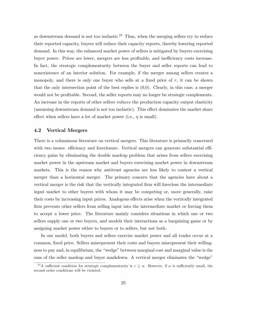
Theorem 10 Consider a vertically separated, intermediate input market with constant cost

and value elasticities and a fixed downstream price. (i) If the seller is a monopolist and there

are at least two buyers, then a vertical merger increases reported demand but not reported

supply so price and output increase. (ii) If the buyer is a monopolist and there are at least

two sellers, then a vertical merger increases reported supply but not reported demand so

output increases and price falls. (iii) If there are at least two sellers and buyers, then a

vertical merger increases reported supply and demand, so output increases.

When the only seller in the market merges with a buyer, it does not change its produc-

tion capacity report but it overstates consumption capacity. It then follows from Lemma

7 that reported demand increases substantially as other buyers respond by increasing their

consumption capacity. Hence, both output and price increases. Similarly, when the only

buyer in the market merges with a seller, reported demand does not change but reported

supply increases, lowering price and increasing output. Thus, a vertical merger in monopoly

or monopsony markets always leads to foreclosure, with the magnitude of the effect depend-

ing upon the elasticities of supply and demand and upon market shares. In markets with

multiple buyers and sellers, the vertically integrated firm increases both capacity reports,

which causes rivals on both sides of the market to increase their capacity reports. Hence,

reported supply and demand increases, output increases, but the impact on price is am-

biguous. Intuitively, the foreclosure effect is important when the vertically integrated firm

is either a large net seller or a large net buyer.

The assumption that the market is vertically separated is crucial to the merger analysis.

A vertical merger in a vertically integrated market can lead to a decrease in reported demand

or supply. The reason is that reported production capacity and consumption capacity are

strategic substitutes for a vertically integrated firm. A similar issue arises with vertical

mergers in wholesale markets. Even if the market is vertically separated, increases in

reported consumption capacity reduces the reported capacity of sellers and increases in

reported production capacity reduces the reported capacity of buyers. Thus, in these cases,

26

the impact of a vertical merger on price and output needs to be computed on a case by case

basis.

5 Identification

Suppose a researcher has data on prices and quantities in a market for t = 1, .., T periods and

wants to use our model to estimate cost and demand parameters. Under what conditions

is the model identified?

In addressing this question, it is useful to begin with the standard model that has

been estimated in numerous empirical studies of market power (e.g., Porter [37], Genesove

and Mullin [13].Clay and Troesken [10]). The model assumes that the market is vertically

separated and that buyers are price-takers. Market demand is given by

pt = P (Qt,Kt, Zt, udt; δ)

where Zt are observed demand shifters, udt represents unobserved (to the researcher) de-

mand shocks that are independent over time, and δ are the unknown demand parameters.

The pricing equation for sellers is specified as

pt = c0(Qt,Wt, ust;φ)− λQt∂P (Qt,Kt, Zt; δ)

∂Q,

where Wt are observed factors that shift marginal cost, ust represents unobserved supply

shocks, and φ are the unknown cost parameters. Here we have assumed that the only

aggregate quantity data are available so c0 is the marginal cost of the average firm. The

parameter λ is known as the “conduct” parameter and interpreted as the average of the

firms’ conjectures on how aggregate supply will change with an increase in their output.

In the Cournot model, rivals cannot react so λ is equal to 1 but, in empirical work, it is

often useful to allow markups to vary from the Cournot markups. As is well known (see

Bresnahan [7]), the above model is identified if instruments are available for the endogenous

variables in the two equations. Shifts in marginal cost can be used to identify the demand

parameters, and shifts in demand and in slope of demand can be used to identify the cost and

conduct parameters. In the various empirical studies surveyed by Bresnahan [7], estimates

of λ range from 0.05 to 0.65. More recently, Genesove and Mullin report estimates of λ for

27

the sugar industry at the turn-of-the-century ranging from 0.038 to 0.10, with the latter

computed directly from the data on prices and marginal costs. Clay and Troesken report

similarly low estimates for λ in the whiskey industry at the turn-of-the-century. These

estimates suggest that dynamic considerations do matter and lead to lower markups.

In our model,

λ =ε

ε+ (1− σ)η

where σ denotes the market share of the average firm. It is not a free parameter but

in general depends upon the elasticities of reported demand and supply evaluated at the

equilibrium market quantity. Note that λ is bounded between 0 and 1, with the upper

bound achieved when η = 0 (i.e., the Cournot case). Hence, our model provides a potential

explanation for why estimated markups are typically lower than Cournot markups.

Our model is identified in vertically separated, intermediate input markets with constant

cost and value elasticities. More precisely, suppose

c0(Qt,Wt, ust) =Wφt Q

1/ηt Γ

−1/ηt ust

and

v0(Qt, Zt, udt) = ZδtQ

−1/εt K

1/εt udt.

where (ust, udt) are distributed multivariate lognormal with mean zero and covariance Σ.

This is the model that Porter estimates under the assumption that buyers are price-takers

which, in terms of our model, means that they are reporting their true capacity. As we

have observed previously, the elasticities of reported demand and supply are constant in

this model, independent of the capacity reports. Furthermore, the argument given for

Lemma 7 also implies that capacity reports of sellers and buyers are independent of the

observed and unobserved factors shifting demand and supply. Thus, as long as actual

capacities are constant over time, Γ and K are constants, as are the firms’ market shares.

This in turn implies that λ is a constant and that the derivative of the reported demand

schedule does not vary with reported buyer capacity. The variation in markups over time is

coming from exogenous variation in the observed and unobserved factors but not from the

endogenous variables, Γ andK. As a result, changes inW shifts the reported supply but not

the reported demand, thereby identifying the demand parameters; changes in Z shifts the

28

reported demand but not the reported supply, thereby identifying the cost parameters.25

Our model is not identified if elasticities (and/or slopes of reported demand and supply)

depend upon reported capacities and these differ from actual capacities due to the exercise

of market power. This will typically be the case in wholesale markets and in vertically

integrated markets. In these markets, markups will be a function of K and Γ, which are

likely to depend upon the unobserved shocks affecting demand and supply. As a result, λ

and P 0 will vary over time and the variation will be correlated with the unobserved shocks.

One could try to find instruments for K and Γ but data on reported capacities are typically

not available.

6 Application: The Exxon-Mobil Merger

Our second application is to a merger of Exxon and Mobil’s gasoline refining and retailing

assets in western United States. The west coast gasoline market is relatively isolated from

the rest of the nation, both because of transportation costs,26 and because of the requirement

of gasoline reformulated for lower emission, a type of gasoline known as CARB.

Available market share data is generally imperfect, because of variations due to shut-

downs and measurement error, and the present analysis should be viewed as an illustration

of the theory rather than a formal analysis of the Exxon-Mobil merger. Nevertheless, we

have tried to use the best available data for the analysis. In Table 1, we provide a list of

market shares, along with our estimates of the underlying capital shares and the post-merger

market shares, which will be discussed below. The data come from Leffler and Pulliam [26].

From Table 1, it is clear that there is a significant market in the intermediate good

of bulk (unbranded) gasoline, prior to branding and the addition of proprietary additives.

However, the actual size of the intermediate good market is larger than one might conclude

25Solving for equilibrium and taking logs, the structural model is given by

logQt =εδη

ε+ ηlogZt −

φεη

ε+ ηlogWt +

ε

ε+ ηlogΓ+

η

ε+ ηlogK +

εη

ε+ ηlog

udtust

logPt =εδ

ε+ ηlogZt +

φη

ε+ ηlogWt −

ε

ε+ ηlogΓ+

1

ε+ ηlogK +

ε

ε+ ηlog

udtust

It is straightforward to show that the structural parameters (ε, η, δ, φ) can be recovered from parameterestimates of the reduced form regressions of logQt and logPt on a constant, logZt and logWt.26There is currently no pipeline permitting transfer of Texas or Louisiana refined gasoline to California,

and the Panama Canal can not handle large tankers, and in any case is expensive. Nevertheless, when pricesare high enough, CARB gasoline has been brought from the Hess refinery in the Caribbean.

29

from Table 1, because firms engage in swaps. Swaps trade gasoline in one region for gasoline

in another. Since swaps are balanced, they will not affect the numbers in Table 1.

It is well known that the demand for gasoline is very inelastic. We consider a base case

of an elasticity of demand, α, of 1/3. We estimate θ to be 0.7, an estimate derived from an

average of 60.1 cents spot price for refined CARB gasoline, out of an average of 85.5 (net

of taxes) at the pump in the year 2000.27 We believe the selling cost to be fairly elastic,

with a best estimate of β = 5. Similarly, by all accounts refining costs are quite inelastic;

we use η = 1/2 as the base case. We will consider the robustness to parameters below, with

α = 1/5, β = 3, and η = 1/3.

Table 2 presents our summary of the Exxon/Mobil merger. The first three columns

provide the assumptions on elasticities that define the four rows of calculations. The fourth

column provides the markups that would prevail under a fully symmetric and balanced

industry, that is, one comprised of fifteen equal sized firms. This is the best outcome that

can arise in the model, given the constraint of fifteen firms, and can be used a benchmark.

The fifth column considers a world without refined gasoline exchange, in which all fifteen

companies are balanced, and is created by averaging production and consumption shares

for each firm. This calculation provides an alternative benchmark for comparison, to assess

the inefficiency of the intermediate good exchange. The next four columns use the existing

market shares, reported in Table 1, as an input, and then compute the price-cost margin

and quantity reduction, pre-merger, post-merger, with a refinery sale, or with a sale of retail

outlets, respectively.

Table 2 does not use the naive approach of combining Exxon and Mobil’s market shares,

an approach employed in the Department of Justice Merger Guidelines. In contrast to the

merger guidelines approach, we first estimate the capital held by the firms, then combine

this capital in the merger, then compute the equilibrium given the post-merger allocation of

capital. The estimates are not dramatically different than those that arise using the naive

approach of the merger guidelines. To model the divestiture of refining capacity, we combine

only the retailing capital of Exxon and Mobil; similarly, to model the sale of retailing, we

combine the refining capacity.

The estimated shares of capital are presented in Table 1. These capital shares reflect

27We will use all prices net of taxes. As a consequence, the elasticity of demand builds in the effect oftaxes, so that a 10% retail price increase (before taxes) corresponds approximately to an 17% increase inthe after tax price. Thus, the elasticity of 1/3 corresponds to an actual elasticity of closer to 0.2.

30

the incentives of large net sellers in the intermediate market to reduce their sales in order to

increase the price, and the incentive of large net buyers to decrease their demand to reduce

the price. Equilon, the firm resulting from the Shell-Texaco merger, is almost exactly

balanced and thus its capital shares are relatively close to its market shares. In contrast, a

net seller in the intermediate market like Chevron refines significantly less than its capital

share, but retails close to its retail capital share. Arco, a net buyer of unbranded gasoline,

sells less than its share from its retail stores, but refines more to its share of refinery capacity.

The estimates also reflect the incentives of all parties to reduce their downstream sales to

increase the price, an incentive that is larger the larger is the retailer.

The sixth column of Table 2 provides the pre-merger markup, or MHI, and is a direct

calculation from equation (24) using the market shares of Table 1. The seventh, eighth

and ninth columns combine Exxon and Mobil’s capital assets in various ways. The seventh

combines both retail and refining capital. The eighth combines retail capital, but leaves

Exxon’s Benicia refinery in the hands of an alternative supplier not listed in the table.

This corresponds to a sale of the Exxon refinery. The ninth and last column considers the

alternative of a sale of Exxon’s retail outlets. (It has been announced that Exxon will sell

both its refining and retailing operations in California.)

Our analysis suggests that without divestiture the merger will, under the hypotheses of

the theory, have a small effect on the retail price. In the base case, the markup increases from

20% to 21%, and the retail price increases 1%.28 Moreover, a sale of a refinery eliminates

most the price increase; the predicted price increase is less than a mil. Unless retailing costs

are much less elastic than we believe, a sale of retail outlets accomplishes very little. The

predicted changes in prices, as a percent of the pre-tax retail price, are summarized in Table

2. The unimportance of retailing is not supported by Hastings [14].

The predicted quantity, as a percentage of the fully efficient quantity, is presented in

Table 2, in parentheses. The first three columns present the prevailing parameters. The

next six columns correspond to the conceptual experiments discussed above. The symmetric

column considers fifteen equal sized firms. The balanced asymmetric column uses the data

of Table 1, but averages the refining and retail market shares to yield a no-trade initial

solution. The pre-merger column corresponds to Table 1; post-merger combines Exxon and

Mobil. Finally, the last two columns consider a divestiture of a refinery and retail assets,

28The percentage increase in the retail price can be computed by noting that p = q−A.

31

respectively. We see the effects of the merger through a small quantity reduction. Again,

we see that a refinery sale eliminates nearly all of the quantity reduction.

The analysis used the computed market shares rather than the approach espoused by

the U.S. Department of Justice Merger Guidelines. Our approach is completely consistent

with the theory, unlike the merger guidelines approach, which sets the post-merger share

of the merging firms to the sum of their pre-merger shares. This is inconsistent with the

theory because the merger will have an impact on all firms’ shares. In Table 1, we provide

our estimate of the post-merger shares along side the pre-merger shares. Exxon and Mobil

were responsible for 18.6% of the refining, and we estimate that the merger will cause them

to contract to 17.4%. The other firms increase their share, though not enough to offset the

combined firm’s contraction.

There is little to be gained by using the naive merger guidelines market shares, because

the analysis is sufficiently complicated to require machine-based computation. However,

we replicated the analysis using the naive market shares, and the outcomes are virtually

identical. Thus, it appears that the naive approach gives the right answer in this application.

7 Conclusion

This paper presents a method for measuring industry concentration in intermediate goods

markets. It is especially relevant when firms have captive consumption, that is, some of the

producers of the intermediate good use some or all of their own production for downstream

sales.

The major advantages of the theory are its applicability to a wide variety of industry

structures, its low informational requirements, and its relatively simple formulae. The major

disadvantages are the special structure assumed in the theory and the static nature of the

analysis. The special structure mirrors Cournot, and thus is subject to the same criticisms

as the Cournot model. For all its defects, the Cournot model remains the standard model

for antitrust analysis; the present theory extends Cournot-type analysis to a new realm.

We considered the application of the theory to wholesale electricity markets and to the

merger of Exxon and Mobil assets in western United States. Several reasonable predictions

emerge. In wholesale electricity markets, firm markups are approximately zero during low

demand periods, high during high demand periods, and vary depending upon the firm’s net

position and market share. In west coast gasoline markets, the industry produces around

32

95% of the efficient quantity and the merger reduces quantity by a small amount, around

0.3%. The price-cost margin is on the order of 20% and rises by a percentage point or

two. A sale of Exxon’s refinery eliminates nearly all of the predicted price increase. This

last prediction arises because retailing costs are relatively elastic, so that firms are fairly

competitive downstream. Thus, the effects of industry concentration arise primarily from

refining, rather than retail. Hence the sale of a refinery (Exxon and Mobil have one refinery

each) cures most of the problem associated with the merger. The naive approach based

purely on market shares gives answers similar to the more sophisticated approach of first

computing the capital levels, combining the capital of the merging parties, then computing

the new equilibrium market shares. Finally, it is worth noting that the computations

associated with the present analysis are straightforward, and run in a few seconds on a

modern PC.

As with Cournot analysis, the static nature of the theory is problematic. In some

industries, entry of new capacity is sufficiently easy that entry would undercut any exercise

of market power. The present theory does not accommodate entry, and thus any analysis

would need a separate consideration of the feasibility and likelihood of timely entry.29 When

entry is an important consideration, the present analysis provides an upper bound on the

ill-effects merger.

Another limitation of the theory is the restriction to homogenous good markets. An

extension of the theoretical approach to markets in which sellers offer differentiated goods

would be challenging but worth exploring.

29McAfee, Simons and Williams [33] present a Cournot-based merger evaluation theory that explicitlyaccommodates entry in the analysis.

33

References

[1] Akgun, Ugur, “Mergers with Supply Functions,” Journal of Industrial Economics,

forthcoming, 2005.

[2] Allaz, B. “Uncertainty and Strategic Forward Transactions”, International Journal of

Industrial Organization, 19, 1992, pp. 297-308.

[3] Bernheim, Douglas, and Michael Whinston, “Multimarket Contact and Collusive Be-

havior,” Rand Journal of Economics, 21, no. 1, Spring, 1990, pp. 1- 26.

[4] Bushnell, James B., Erin T. Mansur, and Celeste Saravia, “Vertical Arrangements,

Market Structure, and Competition: An Analysis of Restructured U.S. Electricity

Markets”, mimeo, 2006.

[5] Borenstein, Severin, and James Bushnell, “An Empirical Analysis of the Potential for

Market Power in California’s Electricity Market”, Journal of Industrial Economics, vol.

47(3), pp. 285-323.

[6] Borenstein, Severin., Bushnell, James and Frank Wolak, “Measuring Market Inefficien-

cies in California’s Restructured Wholesale Electricity Market,” American Economic

Review, December 2002.

[7] Bresnahan, Timothy F., “Empirical Studies of Industries with Market Power” in

Handbook of Industrial Organization, Volume II, edited by R. Schmalensee and

R.D. Willig, New York: North Holland, 1989.

[8] Brunekreeft, G., “A Multiple-Unit, Multiple-Period Auction in the British Electricity

Market”, Energy Economics, vol. 23(1), 2001, pp. 99-118.

[9] de Fontenay, Catherine C. and Joshua Gans, “Vertical Integration in the Presence of

Upstream Competition,” Rand Journal of Economics, forthcoming, 2005.

[10] Clay, Karen andWerner Troesken, “Further Tests of Static Oligopoly Models: Whiskey,

1882-1898,” Journal of Industrial Economics, 2003.

[11] Farrell, Joseph, and Carl Shapiro, “Horizontal Mergers: An Equilibrium Analysis,”

American Economic Review, 80, p.107-26.

34

[12] Gans, Joshua, “Concentration-Based Merger Tests and Vertical Market Structure”,

mimeo, University of Melbourne, 2006.

[13] Genesove, David and Wallace P. Mullin, “Testing Static Oligopoly Models: Conduct

and Cost in the Sugar Industry, 1890-1914,” Rand Journal of Economics, 2, Summer,

1998, pp. 355-377.

[14] Hastings, J., “Vertical Relationships and Competition in Retail Gasoline Markets: Em-

pirical Evidence from Contract Changes in Southern California,” American Economic

Review, March, 2004.

[15] Holmberg, P. “Unique Supply Function Equilibrium with Capacity Constraints”, work-

ing paper, University of Uppsala, Uppsala, Sweden, 2004.

[16] Holmberg, P. “Asymmetric Supply Function Equilibrium with Constant Marginal

Costs”, working paper, University of Uppsala, Uppsala, Sweden, 2005.

[17] Goldberg, P.K. and F. Verboven, “The Evolution of Price Dispersion in European Car

Markets”, Review of Economic Studies, 2001, pp. 811-844

[18] Green, Richard, “Increasing Competition in the British Electricity Spot Market,” Jour-

nal of Industrial Economics, 44, 1996, pp. 205-216.

[19] Green, Richard, “The Electricity Contract Market in England and Wales,” Journal of

Industrial Economics, 47, 1999, pp. 107-124.

[20] Green, Richard and David M. Newberry, “Competition in the British Electricity Spot

Market,” Journal of Political Economy, 100, 1992, pp. 929-953.

[21] Hart, Oliver and Jean Tirole, “Vertical Integration and Market Foreclosure,” Brook-

ings Papers on Economic Activity: Microeconomics, Special Issue, 1990, 205-

76.

[22] Hortecsu, Ali and Steven L. Puller, “Understanding Strategic Bidding in Restructured

Electricity Markets: A Case Study of ERCOT,” mimeo, March 2006.

[23] Klemperer, Paul and Margaret Meyer, “Supply Function Equilibria in Oligopoly Under

Uncertainty,” Econometrica 57, no. 6, November 1989, 1243-77.

35

[24] Kreps, David and Jose Scheinkman, “Quantity Precommitment and Betrand Compe-

tition Yield Cournot Outcomes,” Bell Journal of Economics, 14, no. 2, Autumn 1983,

326-37.

[25] Laussel, D., “Strategic Commercial Policy Revisited: A Supply Function Equilibrium

Model,” American Economic Review, 82, 1992, pp. 84-99.

[26] Leffler, Keith and Barry Pulliam, “Preliminary Report to the California Attorney

General Regarding California Gasoline Prices,” November 22, 1999.

[27] Mahenc, P., and F.Salanie, “Softening Competition through Forward Trading”, Journal

of Economic Theory, 116, 2004, pp. 282-293.

[28] Mansur, Erin T., “Upstream Competition and Vertical Integration in Electricity Mar-

kets”, Journal of Law and Economics, forthcoming.

[29] Manuszak, M.D., “The Effects of Upstream Mergers on Retail Gasoline Markets”,

working paper, Carnegie Mellon University.

[30] McAfee, R. Preston and John McMillan, “Analyzing the Airwaves Auction,” Journal

of Economic Perspectives, 10, no. 1, Winter 1996, 159-75.

[31] McAfee, R. Preston and Michael Williams, “Horizontal Mergers and Antitrust Policy,”

Journal of Industrial Economics, XL, June, 1992, 181-7

[32] McAfee, R. Preston and M. Schwartz, “Opportunism in Multilateral Vertical Contract-

ing: Nondiscrimination, Exclusivity, and Uniformity,” American Economic Review, 84

(1), 1994, pp.210-230..

[33] McAfee, R. Preston, Joseph Simons and Michael Williams, “Horizontal Mergers in

Spatially Differentiated Noncooperative Markets,” Journal of Industrial Economics,

XL, December 1992, 349-57.

[34] McMillan, John, “Selling Spectrum Rights,” Journal of Economic Perspectives, 8, Sum-

mer 1994, 145-62.

[35] Milgrom, Paul, “Game Theory and the Spectrum Auctions,” European Economic Re-

view, 42, May, 1998, pp. 771- 78.

36

[36] Mortimer, J.H., “The Effects of Revenue-Sharing Contracts on Welfare in Vertically

Separated Markets: Evidence from the Video Rental Industry”, working paper, Har-

vard University, 2002.

[37] Porter, R.H., “A Study of Cartel Stability: The joint executive committee, 1880-1886”,

Bell Journal of Economics, 14, 1983, pp. 301-314.

[38] O’Brien, D.P., and Greg Schaffer, “Vertical Control with Bilaternal Contracts,” Rand

Journal of Economics, 23 (3), 1992, pp. 299-308.

[39] Ordover, Janusz, Garth Saloner and Steven Salop, “Equilibrium Vertical Foreclosure,”

American Economic Review, 80, no. 1, March 1990, p. 127-42.

[40] Rey, Patrick and Jean Tirole, “A Primer on Foreclosure,” Handbook of Industrial

Organization, Vol. III, North Holland: Amsterdam, 2003, forthcoming.

[41] Salinger, Michael, “Vertical Mergers and Market Foreclosure,” Quarterly Journal of

Economics, 103, no.2, May 1988, 345-56.

[42] Salop, Steven, and David Scheffman, “Cost Raising Strategies,” Journal of Industrial

Economics, 36, no.1, September 1987, 19-34.

[43] Segal, Igal, “Contracting with Externalities,” Quarterly Journal of Economics, 114 (2),

1999, pp. 337-388.

[44] Sweeting, Andrew, “Market Power in the England and Wales Wholesale Electricity

Market 1995-2000”, mimeo, October, 2005.

[45] Villa-Boas, J.M., and Y. Zhao, “Retailers, Manufacturers, and Individual Consumers:

Modeling the Supply Side in Ketchup Marketplace”, Journal of Marketing Research,

forthcoming.

[46] Villa-Boas, S.B., “Vertical Contracts Between Manufacturers and Retailers: Inference

with Limited Data”, CUDARE working paper 943, UC-Berkeley, 2005

[47] Villa-Boas, S.B. and R. Hellerstein, “Identification of Supply Models of Retailer and

Manufacturer Oligopoly Pricing”, Economics Letters, 90, N.1, pp.132-140.

37

[48] Wolak, Frank, “An Empirical Analysis of the Impact of Hedge Contracts on Bidding

Behavior in a Competitive Electricity Market”, International Economic Review, vol.

14(2), 2000, pp. 1-39.

[49] Wolak, Frank, “Measuring Unilateral Market Power in Wholesale Electricity Markets:

The California Market, 1998-2000”, American Economic Review, May, 2003, pp. 425-

430.

[50] Wolak, Frank, “Identification and Estimation of Cost Functions Using Observed Bid

Data: An Application to Electricity Markets”, in Advances in Economics and

Econometrics: Theory and Applications, (M. Dewatripont, L.P. Hansen, and S.J.

Turnovsky, eds.), Eighth World Congress, Vol. II, New York: Cambridge University

Press, 2003, pp. 133-69.

[51] Wolak, Frank, “Quantifying the Supply-Side Benefits from Forward Contracting in

Wholesale Electricity Markets”, mimeo, November, 2004.

[52] Wolfram, Catherine D., “Measuring Duopoly Power in the British Electricity Spot

Market”, American Economic Review, vol. 89(4), 1999, pp. 805-826.

[53] U.S. Department of Justice Merger Guidelines.

38

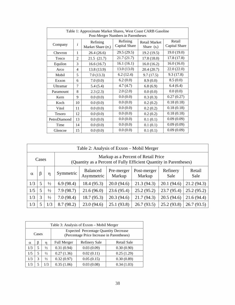
38

Table 1: Approximate Market Shares, West Coast CARB Gasoline Post-Merger Numbers in Parentheses

Company i Refining Market Share (σi)

Refining Capital Share

Retail Market Share (si)

Retail Capital Share

Chevron 1 26.4 (26.6) 29.5 (29.5) 19.2 (19.5) 19.0 (19.0) Tosco 2 21.5 (21.7) 21.7 (21.7) 17.8 (18.0) 17.8 (17.8)

Equilon 3 16.6 (16.7) 16.1 (16.1) 16.0 (16.2) 16.0 (16.0) Arco 4 13.8 (13.9) 13.0 (13.0) 20.4 (20.7) 22.0 (22.0) Mobil 5 7.0 (13.3) 6.2 (12.4) 9.7 (17.5) 9.3 (17.8) Exxon 6 7.0 (0.0) 6.2 (0.0) 8.9 (0.0) 8.5 (0.0)

Ultramar 7 5.4 (5.4) 4.7 (4.7) 6.8 (6.9) 6.4 (6.4) Paramount 8 2.3 (2.3) 2.0 (2.0) 0.0 (0.0) 0.0 (0.0)

Kern 9 0.0 (0.0) 0.0 (0.0) 0.3 (0.3) 0.27 (0.27) Koch 10 0.0 (0.0) 0.0 (0.0) 0.2 (0.2) 0.18 (0.18) Vitol 11 0.0 (0.0) 0.0 (0.0) 0.2 (0.2) 0.18 (0.18)

Tesoro 12 0.0 (0.0) 0.0 (0.0) 0.2 (0.2) 0.18 (0.18) PetroDiamond 13 0.0 (0.0) 0.0 (0.0) 0.1 (0.1) 0.09 (0.09)

Time 14 0.0 (0.0) 0.0 (0.0) 0.1 (0.1) 0.09 (0.09) Glencoe 15 0.0 (0.0) 0.0 (0.0) 0.1 (0.1) 0.09 (0.09)

Table 2: Analysis of Exxon – Mobil Merger

Cases Markup as a Percent of Retail Price (Quantity as a Percent of Fully Efficient Quantity in Parentheses)

α β η Symmetric Balanced Asymmetric

Pre-merger Markup

Post-merger Markup

Refinery Sale

Retail Sale

1/3 5 ½ 6.9 (98.4) 18.4 (95.3) 20.0 (94.6) 21.3 (94.3) 20.1 (94.6) 21.2 (94.3)1/5 5 ½ 7.9 (98.7) 21.6 (96.0) 23.6 (95.4) 25.2 (95.2) 23.7 (95.4) 25.2 (95.2)1/3 3 ½ 7.0 (98.4) 18.7 (95.3) 20.3 (94.6) 21.7 (94.3) 20.5 (94.6) 21.6 (94.4)1/3 5 1/3 8.7 (98.2) 23.0 (94.6) 25.1 (93.8) 26.7 (93.5) 25.2 (93.8) 26.7 (93.5)

Table 3: Analysis of Exxon – Mobil Merger

Cases Expected Percentage Quantity Decrease

(Percentage Price Increase in Parentheses)

α β η Full Merger Refinery Sale Retail Sale 1/3 5 ½ 0.31 (0.94) 0.03 (0.09) 0.30 (0.90) 1/5 5 ½ 0.27 (1.36) 0.02 (0.11) 0.25 (1.29) 1/3 3 ½ 0.32 (0.97) 0.05 (0.15) 0.30 (0.89) 1/3 5 1/3 0.35 (1.06) 0.03 (0.08) 0.34 (1.03)

39

Appendix

Proof of Theorems 1 and 3: Before proceeding, note that differentiating the equilibrium condition in equation (7) implies that

.)(,, 11

1

11

1

11

1

−−

−

−−

−

−−

−

+=

Γ∂∂

⎟⎠⎞

⎜⎝⎛ Γ−=

∂∂

⎟⎠⎞

⎜⎝⎛

+=

Γ∂∂

⎟⎟⎠

⎞⎜⎜⎝

⎛ Γ+

=∂∂

⎟⎟⎠

⎞⎜⎜⎝

⎛ηε

ηεηε

ηηε

ε PPK

PPKandQ

QKQ

QK

Differentiating the firm’s profit function in equation (8) and substituting the relations given above yields the following first order conditions:

KpsQ

KQQ

cpKQs

Kk

KQp

kQs

vk iii

i

ii

i

i

i

i

i

∂∂

−−⎟⎠⎞

⎜⎝⎛

∂∂

⎟⎟⎠

⎞⎜⎜⎝

⎛⎟⎟⎠

⎞⎜⎜⎝

⎛′−+⎟

⎟⎠

⎞⎜⎜⎝

⎛

∂∂

+⎟⎟⎠

⎞⎜⎜⎝

⎛−⎟

⎟⎠

⎞⎜⎜⎝

⎛−⎟⎟

⎠

⎞⎜⎜⎝

⎛′=

∂

∂)(

ˆ1ˆ 2 σσ

γσπ

( ) ( ) ( ) ⎥⎦

⎤⎢⎣

⎡

+−−⎟⎟

⎠

⎞⎜⎜⎝

⎛+

′−+⎟⎟⎠

⎞⎜⎜⎝

⎛+

+−−′= −−

−

−−

−

−−

−

11

1

11

1

11

1 )()(1ηε

ηεσηε

εσηε

εiiiiiii spcpsspv

KQ .

Similarly,

Γ∂∂

−−⎟⎟⎠

⎞⎜⎜⎝

⎛Γ∂

∂+⎟

⎠⎞

⎜⎝⎛

Γ−

Γ⎟⎟⎠

⎞⎜⎜⎝

⎛⎟⎟⎠

⎞⎜⎜⎝

⎛′−+⎟

⎠⎞

⎜⎝⎛

Γ∂∂

⎟⎟⎠

⎞⎜⎜⎝

⎛−⎟⎟

⎠

⎞⎜⎜⎝

⎛′=

∂∂ psQQQ

QcpQsp

kQs

v iiii

i

ii

i

i

i

i )(ˆ1

ˆ 2 σσγ

γσ

γπ

( ) ( ) ⎥⎦

⎤⎢⎣

⎡

+−+⎟⎟

⎠

⎞⎜⎜⎝

⎛+

+−′−+⎟⎟⎠

⎞⎜⎜⎝

⎛+

−′Γ

= −−

−

−−

−

−−

−

11

1

11

1

11

1 )()(1ηε

ηεσηε

ησσηε

ηiiiiiii spcpspvQ .

Thus,

iii

i

i

i cvQkQ

K ′−′=∂∂Γ

+∂

∂γππˆˆ .

In an interior equilibrium, then, .0=′−′ ii cv Either of the first order conditions yields (15). The Case of si=0, σi>0. If σi>0, the first order condition on iγ̂ holds with equality. Consequently, using si=0,

( ) ⎥⎦

⎤⎢⎣

⎡

+−+⎟⎟

⎠

⎞⎜⎜⎝

⎛+

+−′−Γ

= −−

−

−−

−

11

1

11

1 )()0(10ηε

ηεσηε

ησσ iiii pcpQ

This yields

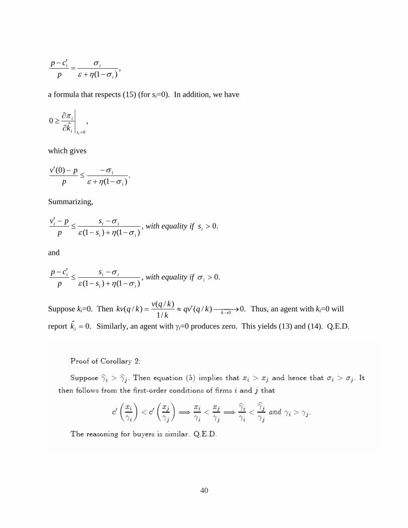
40

,)1( i

ii

pcp

σηεσ−+

=′−

a formula that respects (15) (for si=0). In addition, we have

,ˆ00=

∂

∂≥

isi

i

kπ

which gives

.)1(

)0(

i

i

ppv

σηεσ−+

−≤

−′

Summarizing,

.0,)1()1(

>−+−

−≤

−′i

ii

iii sifequalitywithss

ppv

σηεσ

and

.0,)1()1(

>−+−

−≤

′−i

ii

iii ifequalitywithss

pcp

σσηε

σ

Suppose ki=0. Then .0)/(/1

)/()/( 0⎯⎯→⎯′≈= →kkqvqkkqvkqkv Thus, an agent with ki=0 will

report .0ˆ =ik Similarly, an agent with γi=0 produces zero. This yields (13) and (14). Q.E.D.

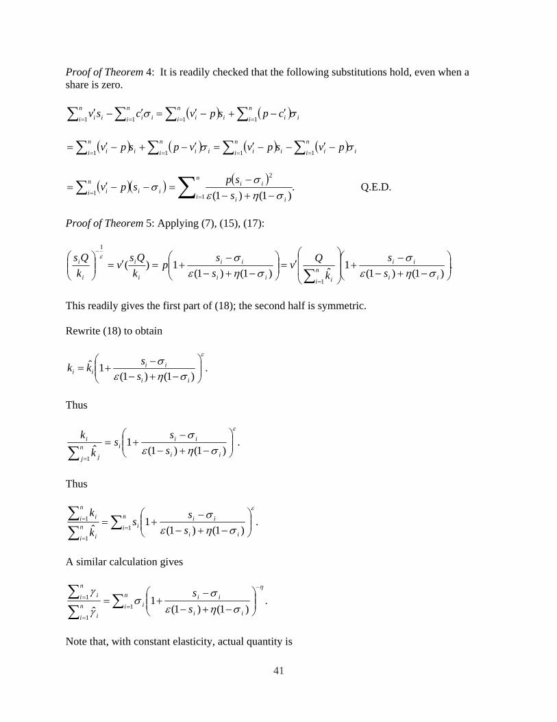
41

Proof of Theorem 4: It is readily checked that the following substitutions hold, even when a share is zero.

in

i iin

i i csv σ∑∑ ==′−′

11( ) ( ) i

n

i iin

i i cpspv σ∑∑ ==′−+−′=

11

( ) ( ) i

n

i iin

i i vpspv σ∑∑ ==′−+−′=

11( ) ( ) i

n

i iin

i i pvspv σ∑∑ ==−′−−′=

11

( )( )iin

i i spv σ−−′= ∑ =1

( ).

)1()1(1

2

∑= −+−−

=n

i ii

ii

ssp

σηεσ

Q.E.D.

Proof of Theorem 5: Applying (7), (15), (17):

.)1()1(

1ˆ)1()1(

1)(1

1

⎟⎟⎠

⎞⎜⎜⎝

⎛−+−

−+⎟

⎟

⎠

⎞

⎜⎜

⎝

⎛′=⎟⎟

⎠

⎞⎜⎜⎝

⎛−+−

−+=′=⎟⎟

⎠

⎞⎜⎜⎝

⎛

∑ =

−

ii

iin

i iii

ii

i

i

i

i

ss

kQv

ss

pkQs

vkQs

σηεσ

σηεσε

This readily gives the first part of (18); the second half is symmetric. Rewrite (18) to obtain

.)1()1(

1ˆε

σηεσ

⎟⎟⎠

⎞⎜⎜⎝

⎛−+−

−+=

ii

iiii s

skk

Thus

.)1()1(

1ˆ

1

ε

σηεσ

⎟⎟⎠

⎞⎜⎜⎝

⎛−+−

−+=

∑ =ii

iiin

j j

i

ss

sk

k

Thus

.)1()1(

1ˆ 1

1

1 ∑∑∑

=

=

=⎟⎟⎠

⎞⎜⎜⎝

⎛−+−

−+=

n

iii

iiin

i i

n

i i

ss

sk

k ε

σηεσ

A similar calculation gives

.)1()1(

1ˆ 1

1

1 ∑∑∑

=

−

=

=⎟⎟⎠

⎞⎜⎜⎝

⎛−+−

−+=

n

iii

iiin

i i

n

i i

ss

η

σηεσ

σγ

γ

Note that, with constant elasticity, actual quantity is

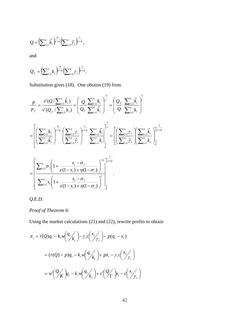
42

( ) ( ) ,ˆˆ11

ηεε

ηεη

γ +=

+= ∑∑=

n

i in

i ikQ and

( ) ( ) .11

ηεε

ηεη

γ +=

+= ∑∑=

n

i in

i if kQ Substitution gives (18). One obtains (19) from

εε1

1

1

1

1

1

1

1ˆ

ˆ)/(

)ˆ/(⎟⎟

⎠

⎞

⎜⎜

⎝

⎛=⎟

⎟

⎠

⎞

⎜⎜

⎝

⎛=

′

′=

∑∑

∑∑

∑∑

=

=

−

=

=

=

=n

i i

n

i ifn

i i

n

i i

fn

i if

n

i i

f k

kQ

Q

k

kQQ

kQv

kQvpp

ηεε

ηεε

ηεη

γ

γ

γ

γ +

=

=

=

=

=

=+

=

=+

=

=

⎥⎥

⎦

⎤

⎢⎢

⎣

⎡

⎟⎟

⎠

⎞

⎜⎜

⎝

⎛

⎟⎟

⎠

⎞

⎜⎜

⎝

⎛=

⎥⎥⎥

⎦

⎤

⎢⎢⎢

⎣

⎡

⎟⎟

⎠

⎞

⎜⎜

⎝

⎛

⎟⎟

⎠

⎞

⎜⎜

⎝

⎛=

∑∑

∑∑

∑∑

∑∑

∑∑

1

1

1

1

1

1

1

1

1

1

1

1ˆ

ˆ

ˆ

ˆˆ n

i i

n

i in

i i

n

i in

i i

n

i in

i i

n

i in

i i

n

i i

k

k

k

k

k

k

.

)1()1(1

)1()1(1

1

1

1

ηε

ε

η

σηεσ

σηεσ

σ+

=

=

−

⎥⎥⎥⎥⎥

⎦

⎤

⎢⎢⎢⎢⎢

⎣

⎡

⎟⎟⎠

⎞⎜⎜⎝

⎛−+−

−+

⎟⎟⎠

⎞⎜⎜⎝

⎛−+−

−+

=

∑

∑

n

iii

iii

n

iii

iii

ss

s

ss

Q.E.D. Proof of Theorem 6: Using the market calculations (21) and (22), rewrite profits to obtain

)()( iii

ii

i

iiii xqpxck

qwkqQr −−⎟⎠⎞⎜

⎝⎛−⎟

⎠⎞⎜

⎝⎛−= γγπ

⎟⎠⎞⎜

⎝⎛−+⎟

⎠⎞⎜

⎝⎛−−=

i

iii

i

iii

xcpxkqwkqpQr γγ))((

⎟⎠⎞⎜

⎝⎛−⎟

⎠⎞⎜

⎝⎛

Γ′+⎟⎠⎞⎜

⎝⎛−⎟

⎠⎞⎜

⎝⎛′=

i

ii

i

iii

xcxQckqwkqK

Qw γ

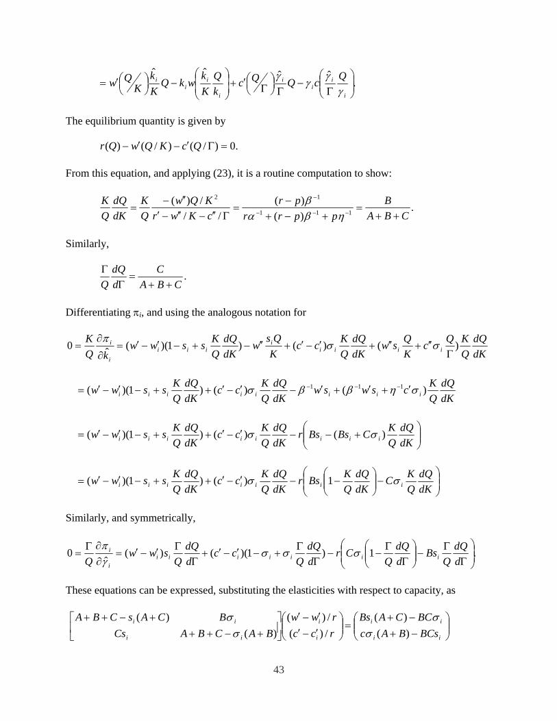
43

.ˆˆˆˆ

⎟⎟⎠

⎞⎜⎜⎝

⎛Γ

−Γ

⎟⎠⎞⎜

⎝⎛

Γ′+⎟⎟⎠

⎞⎜⎜⎝

⎛−⎟

⎠⎞⎜

⎝⎛′=

i

ii

i

i

ii

i QcQQckQ

Kk

wkQKk

KQw

γγ

γγ

The equilibrium quantity is given by .0)/()/()( =Γ′−′− QcKQwQr From this equation, and applying (23), it is a routine computation to show:

.)()(

///)(

111

12

CBAB

pprrpr

cKwrKQw

QK

dKdQ

QK

++=

+−+−

=Γ′′−′′−′

′′−= −−−

−

ηβαβ

Similarly,

.CBA

CddQ

Q ++=

ΓΓ

Differentiating πi, and using the analogous notation for

dKdQ

QKQc

KQsw

dKdQ

QKcc

KQs

wdKdQ

QKssww

kQK

iiiii

iiii

i )()()1)((ˆ0Γ

′′+′′+′−′+′′−+−′−′=∂

∂= σσ

π

dKdQ

QKcswsw

dKdQ

QKcc

dKdQ

QKssww iiiiiiii )()()1)(( 111 σηββσ ′+′+′−′−′++−′−′= −−−

⎟⎟⎠

⎞⎜⎜⎝

⎛+−−′−′++−′−′=

dKdQ

QKCBsBsr

dKdQ

QKcc

dKdQ

QKssww iiiiiiii )()()1)(( σσ

⎟⎟⎠

⎞⎜⎜⎝

⎛−⎟⎟

⎠

⎞⎜⎜⎝

⎛−−′−′++−′−′=

dKdQ

QKC

dKdQ

QKBsr

dKdQ

QKcc

dKdQ

QKssww iiiiiii σσ 1)()1)((

Similarly, and symmetrically,

.1)1)(()(ˆ

0 ⎟⎟⎠

⎞⎜⎜⎝

⎛Γ

Γ−⎟⎟

⎠

⎞⎜⎜⎝

⎛Γ

Γ−−

ΓΓ

+−′−′+Γ

Γ′−′=∂∂Γ

=ddQ

QBs

ddQ

QCr

ddQ

Qcc

ddQ

Qsww

Q iiiiiiii

i σσσγπ

These equations can be expressed, substituting the elasticities with respect to capacity, as

⎟⎟⎠

⎞⎜⎜⎝

⎛−+−+

=⎟⎟⎠

⎞⎜⎜⎝

⎛′−′′−′

⎥⎦

⎤⎢⎣

⎡+−++

+−++

ii

ii

i

i

ii

ii

BCsBAcBCCABs

rccrww

BACBACsBCAsCBA

)()(

/)(/)(

)()(

σσ

σσ

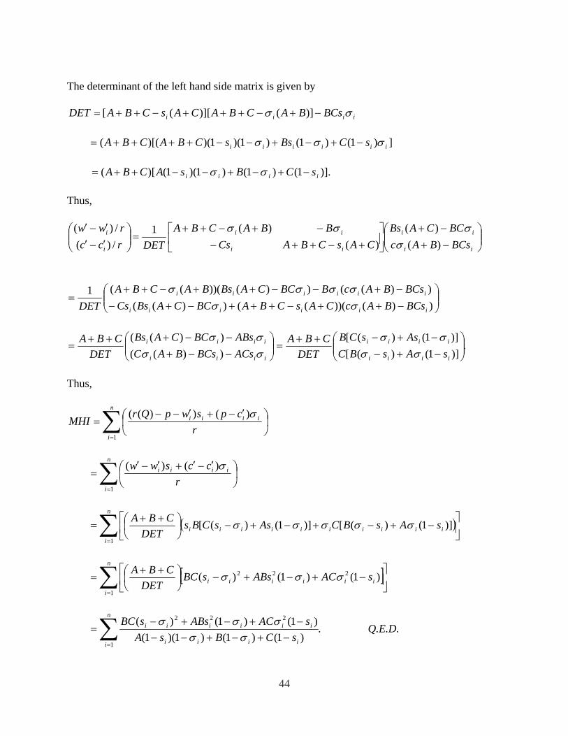
44

The determinant of the left hand side matrix is given by

iiii BCsBACBACAsCBADET σσ −+−+++−++= )]()][([

])1()1()1)(1)()[(( iiiiii sCBssCBACBA σσσ −+−+−−++++=

)].1()1()1)(1()[( iiii sCBsACBA −+−+−−++= σσ Thus,

⎟⎟⎠

⎞⎜⎜⎝

⎛−+−+

⎥⎦

⎤⎢⎣

⎡+−++−

−+−++=⎟⎟

⎠

⎞⎜⎜⎝

⎛′−′′−′

ii

ii

ii

ii

i

i

BCsBAcBCCABs

CAsCBACsBBACBA

DETrccrww

)()(

)()(1

/)(/)(

σσσσ

⎟⎟⎠

⎞⎜⎜⎝

⎛−++−+++−+−−+−−++−++

=))())((())(())(())())(((1

iiiiii

iiiiii

BCsBAcCAsCBABCCABsCsBCsBAcBBCCABsBACBA

DET σσσσσσ

⎟⎟⎠

⎞⎜⎜⎝

⎛−−+−−+++

=iiii

iiii

ACsBCsBACABsBCCABs

DETCBA

σσσσ

))(())((

.)]1()([)]1()([⎟⎟⎠

⎞⎜⎜⎝

⎛−+−−+−++

=iiii

iiii

sAsBCAssCB

DETCBA

σσσσ

Thus,

∑=

⎟⎠⎞

⎜⎝⎛ ′−+′−−

=n

i

iiii

rcpswpQr

MHI1

)())(( σ

∑=

⎟⎠⎞

⎜⎝⎛ ′−′+′−′

=n

i

iiii

rccsww

1

)()( σ

( )∑=

⎥⎦

⎤⎢⎣

⎡−+−+−+−⎟

⎠⎞

⎜⎝⎛ ++

=n

i

iiiiiiiiii sAsBCAssCBsDET

CBA

1

)]1()([)]1()([ σσσσσ

[ ]∑=

⎥⎦

⎤⎢⎣

⎡−+−+−⎟

⎠⎞

⎜⎝⎛ ++

=n

i

iiiiii sACABssBCDET

CBA

1

222 )1()1()( σσσ

.)1()1()1)(1(

)1()1()(

1

222

∑=

−+−+−−−+−+−

=n

i iiii

iiiiii

sCBsAsACABssBC

σσσσσ

Q.E.D.

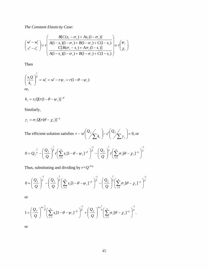
45

The Constant Elasticity Case:

.

)1()1()1)(1()]1()([

)1()1()1)(1()]1()([

⎟⎟⎠

⎞⎜⎜⎝

⎛≡

⎟⎟⎟⎟

⎠

⎞

⎜⎜⎜⎜

⎝

⎛

−+−+−−−+−

−+−+−−−+−

=⎟⎟⎠

⎞⎜⎜⎝

⎛′−′′−′

i

i

iiii

iiii

iiii

iiii

i

i r

sCBsAsAsBC

sCBsAAssCB

rccww

χψ

σσσσσσ

σσ

Then

)1(

1

iiii

i rrwwkQs

ψθψβ

−−=−′=′=⎟⎟⎠

⎞⎜⎜⎝

⎛

or,

βψθ −−−= )]1([ iii rQsk Similarly,

ηχθσγ −−= )]([ iii rQ

The efficient solution satisfies ,0=⎟⎟⎠

⎞⎜⎜⎝

⎛′−⎟⎟⎠

⎞⎜⎜⎝

⎛′− ∑∑ i

f

i

f QckQwr γ or

ηη

ηββ

βα χθσψθ

1

1

11

1

11

][]1[0

−

=

−

−

=

−−⎟⎠

⎞⎜⎝

⎛−⎟⎟

⎠

⎞⎜⎜⎝

⎛−⎟

⎠

⎞⎜⎝

⎛−−⎟⎟

⎠

⎞⎜⎜⎝

⎛−= ∑∑

n

iii

fn

iii

ff r

QQ

srQ

QQ

Thus, substituting and dividing by r=Q-1/α

ηη

ηββ

βαχθσψθ

1

1

11

1

11

][]1[0

−

=

−

−

=

−

−

⎟⎠

⎞⎜⎝

⎛−⎟⎟

⎠

⎞⎜⎜⎝

⎛−⎟

⎠

⎞⎜⎝

⎛−−⎟⎟

⎠

⎞⎜⎜⎝

⎛−⎟⎟

⎠

⎞⎜⎜⎝

⎛= ∑∑

n

iii

fn

iii

ff

QQ

sQ

QQ

Q

or

.][]1[1

1

1

11

1

1η

ηηβ

ββ

χθσψθ

−

=

−

+−

=

−

+

⎟⎠

⎞⎜⎝

⎛−⎟⎟

⎠

⎞⎜⎜⎝

⎛+⎟

⎠

⎞⎜⎝

⎛−−⎟⎟

⎠

⎞⎜⎜⎝

⎛= ∑∑

n

iii

Af

n

iii

Af

QQ

sQ

Q

or

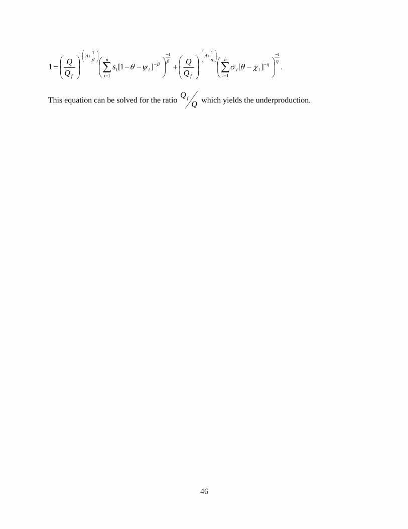
46

.][]1[1

1

1

11

1

1

ηη

ηββ

β

χθσψθ

−

=

−⎟⎟⎠

⎞⎜⎜⎝

⎛+−−

=

−⎟⎟⎠

⎞⎜⎜⎝

⎛+−

⎟⎠

⎞⎜⎝

⎛−⎟

⎟⎠

⎞⎜⎜⎝

⎛+⎟

⎠

⎞⎜⎝

⎛−−⎟

⎟⎠

⎞⎜⎜⎝

⎛= ∑∑

n

iii

A

f

n

iii

A

f QQs

QQ

This equation can be solved for the ratio QQ f which yields the underproduction.

Proof of Theorem 7: First, we need to define a couple of elasticities. Differentiating

the equilibrium condition

Q1α =

µQ

Γ

¶1η

with respect to Γ yields the supply elasticity

Γ

Q

∂Q

∂Γ=

α

η + α.

Similarly, define the equilibrium price elasticity

Γ

p

∂p

∂Γ=−1

η + α.

Differentiating firm i’s profits with respect to its capacity report and substituting the above

elasticities into the first order condition, we obtain

0 =∂p

∂Γ[Qσi − qi] + p

∂Q

∂Γσi + pQ

∙1

Γ− bviΓ

¸− c0i

∙µ1

Γ− bviΓ

¶X + σi

∂Q

∂Γ

¸=

∂p

∂Γ

Γ

p[σi − si] +

p− c0ip

∙∂Q

∂Γ

Γ

Qσi + (1− σi)

¸=−(σi − si)

η + α.+

(p− c0i)

p

∙η(1− σi) + α

η + α

¸.

Q.E.D.

Proof of Theorem 9: Let bv∗i denote the equilibrium pre-merger reports and let Γ∗−12 =nPi=2bv∗i denote the aggregate capacity reported by sellers 2 through n. Define z12 =

bv12v1

and

assume, without loss of generality, that v1 ≥ v2. Fixing its rival reports to their pre-merger

levels, the merged firm’s equilibrium best reply solves

z12(ν1 + v2)−1Γ∗−12 + z12

µεη + αη

εη + αη + αε

¶=

1− z1η12"

η+1η − z

1η12

# .The fact that

(ν1 + v2)−1Γ∗−12 < v−11

¡Γ∗−12 + bv∗2¢

implies that z12 <bv∗1v1. Hence,

bv12ν1 + v2

<bv∗1v1=⇒ bv12 < bv∗1

v1(v1 + v2) < bv∗1 + bv∗2

47

where the last inequality follows from Lemma 1. Thus, the merging firms best reply to its

rival’s pre-merger capacity reports is to reduce its reported total capacity. The result then

follows from Lemma 8. Q.E.D.

Proof of Theorem 10:

Consider a vertical merger between a seller, firm 1, and a buyer, firm 2, in a vertically

separated market. Using market clearing conditions to solve for Q(Γ,K), the optimization

problem for the vertically integrated firm can be expressed as follows:

maxbν12,bk12 Γ−(η+1)ε+η K

η+1ε+η

"bν12 −µ η

η + 1

¶ν−1η1 bν η+1η12

#+Γ

ε−1ε+ηK

− (ε−1)ε+η

∙µε

ε− 1

¶k1ε2bk ε−1ε12 − bk12¸ .

The first-order conditions can be expressed as follows:µη

ε+ η

¶ bν12Γ

"η + 1

η− bν 1η12ν−1η1

#−

⎡⎣1−µbν12ν1

¶ 1η

⎤⎦ = µ ε

ε+ η

¶ bk12K

∙k1ε2bk−1ε12 −µε− 1ε

¶¸µ

ε

ε+ η

¶ bk12K

∙k1ε2bk−1ε12 −µε− 1ε

¶¸−∙k1ε2bk−1ε12 − 1¸ = µ η

ε+ η

¶ bν12Γ

"η + 1

η− ν

−1η1 bν 1η12

#.

Combining the two equations, we find that

1−µbν12ν1

¶1η= −

⎡⎣µ k2bk12¶1

ε− 1

⎤⎦ .Thus, the best reply of the vertically integrated firm is to understate its capacity on one

side of the market and overstate its capacity on the other side of the market. Solving then

yields

k2bk12 =µbν12ν1

¶ εη.

Substitutiting out the consumption capacity ratio, the vertically integrated first order

conditions reduces to a single equation

µη

ε+ η

¶µz12

v−11 Γ−12 + z12

¶"η + 1

η− z

1η12

#−"1− z

1η12

#=

µε

ε+ η

¶z− εη

12

k−12 K−12 + z− εη

12

"z1η12 −

µε− 1ε

¶#

Let H denote the LHS expression and G denote the RHS. It is easily verified that both

functions are strictly increasing in z on the unit interval. We denote post-merger equilibrium

reports using the superscript ∗∗.

48

(i) If there is only one seller, then

H(z) = −µε− 1ε+ η

¶+

µε

ε+ η

¶z1η .

Let z∗1 denote the equilibrium report of firm 1 prior to the merger. It solves H(z) = 0 which

implies

z∗1 =

µε− 1ε

¶η

.

But then G(z∗1,K−12) = 0, so z∗∗12 = z∗1 . Furthermore, by Lemma 7, the solution is indepen-

dent of the independent buyers’ capacity reports. Thus, vertical integration has no effect on

the vertically integrated firm’s reported production capacity and its consumption capacity

report is given by

kbk∗∗ =µε− 1ε

¶1ε

which implies that bk∗∗ is larger than k and hence larger than bk∗. From Lemma 7, inde-

pendent buyers respond by increasing their capacity reports. As a result, reported demand

shifts out, output increases, price rises, and the market share of the independent buyers

fall.

(ii) If there is only one buyer, then the solution to H(z,Γ∗∗−12) = G(z) is

z∗∗12 =

µη + 1

η

¶η

,

which implies thatkbk∗∗ =

µη + 1

η

¶ε

.

But it is easily verified that this is also the solution to the monopoly buyer’s first order

condition prior to the merger. Thus, the merger causes the vertically integrated firm to

increase its reported production capacity but reported consumption capacity is unchanged.

From Lemma 7, independent sellers respond by increasing their capacity reports. As a

result, reported supply shifts out, output increases, price falls, and the market share of the

independent sellers fall.

(iii) If there is at least two buyers and sellers, then the solution to the first order condition

of the merged firm,

z∗∗12 ∈∙µ

ε− 1ε

¶η

,

µη + 1

η

¶ε¸

49

since

H

µµε− 1ε

¶η

,Γ∗∗−12

¶< G

µµε− 1ε

¶η

,K∗∗−12

¶= 0

and

H

µµη + 1

η

¶ε

,Γ∗∗−12

¶> G

µµη + 1

η

¶ε

,K∗∗−12

¶> 0,

and both functions are increasing on this interval. Thus, G(z∗∗12 ,K∗∗−12) > 0 which implies

that

H(z∗∗12 ,Γ∗∗−12) > 0 = H(z∗1 ,Γ

∗−12).

which is consistent with Lemma 7 if and only if z∗∗12 > z∗1 and Γ∗∗−12 > Γ∗−12. Hence, the

vertical merger causes the merged firm to increase its reported production and consumption

capacity. Independent buyers and sellers also increase their reported capacity. Q.E.D.

50