A Theory of Liquidity, Investment and Credit Risk for Financially Constrained

Firms 1

Aaditya Iyer 2

March 29, 2016

Preliminary and Incomplete.

Abstract

This paper builds a dynamic capital structure model of the firm to understand how liquidity

management, investment policy and strategic default risk interact with each other in a unified

framework in the presence of costly external financing and permanent shocks to firm capital

stock. The model features both solvency and liquidity channels of default, in line with the

data, and its tractability helps to quantify the effect of these different channels of default on

firm’s contingent claims. Equity holders choose optimal default, dividend, equity issuance and

investment policies. Investment takes the form of a real option and firm investment policy is

a function of both capital and cash and depends on distance to default. If a firm is financially

constrained before investing, but unconstrained after investing, then the level of cash needed

to invest is decreasing as a function of firm capital stock. On the other hand, if the firm is

unconstrained both before and after investing, then cash serves as a complement to capital

during investment. An increase in volatility of the investment project results in increased

liquidity holdings, lower dividends and lower equity value even prior to investment - contrary

to standard growth option literature. Costly external financing lowers the optimal leverage

choice of firms, and may explain the “debt conservatism puzzle”.

1I am very grateful to my advisors Viral Acharya and Xavier Gabaix for their continued advice andsupport. I would like to thank Thomas Philippon, Alexi Savov and Rangarajan Sundaram for their numerouscomments and suggestions. I have also benefited from conversations with Jennifer Carpenter, EduardoDavila, Stijn van Nieuwerburgh, Vadim Elenev and Mohsan Bilal.

2Affiliation: NYU Stern School of Business

1

1 Introduction:

Financial distress and capital market frictions are a fundamental driver of firms’ leverage,

liquidity and investment policies. According to standard corporate finance theory, firms op-

erate in frictionless capital markets and trade off the tax benefits of debt against the distress

costs associated with bankruptcy when choosing optimal leverage. Firms also determine

when to invest by trading off the future revenue and uncertainty associated with investment

against the cost to finance investment. In reality, however, firms do not operate in frictionless

capital markets and face significant external financing costs, thereby distorting leverage and

investment policies relative to the frictionless benchmark. In response, firms hold cash as a

hedge against bad shocks, to fund investments and to not have to raise liquidity from capital

markets in those states of the world where earnings alone are not sufficient to pay off debt.

Liquid funds held by the firm, however, carry a liquidity premium, and earn a lower rate

of return than other assets. Firms trade off the costs associated with holding liquid assets

against the flexibility that these assets offer in meeting short term liabilities without having

to incur the cost of raising new equity or restructuring debt, allowing for a rich liquidity

management policy. Graham and Harvey (2001,2002) document the importance that CFO’s

attach to holding liquid assets to increase financial flexibility, reflecting the presence of

external financing costs associated with new equity issuances.

For a levered firm, the liquidity management and investment policies are also affected

by the firm’s credit risk. For a firm close to bankruptcy, every additional dollar of liquidity

is highly valued, delaying investment and postponing dividend payments, thereby affecting

the prices of equity and debt. In this paper, I look to embed a dynamic model of liquidity

and investment into a structural credit risk model of the firm. This allows me to understand

how a firm’s liquidity, investment and default policies jointly interact with each other.

Most existing structural credit risk models ignore the external costs of financing. This

results in a trivial cash policy. Since cash earns a lower rate of return inside the firm, and

since there is no cost to raising liquid funds from external markets, firms find it optimal to

hold no cash and distribute all accrued earnings as dividends.

Under the presence of costly external financing, a firm faces two related sources of risk

- solvency and liquidity. Solvency risk for a firm is the risk that the firm’s financial health

and economic prospects decline. This may be due to the emergence of a competitor, or due

to a decline in fortune of the firm’s industry as a whole. Liquidity risk is the risk that the

firm runs out of cash and will be penalized by having to raise external finance. In practice,

however, a firm’s liquidity policy is tightly dependent on its financial health which is captured

2

by its solvency.

In the absence of frictions to raise external financing, default is only triggered due to

insolvency. Assuming that the firm is hit by a sequence of bad productivity shocks, then

if these shocks are persistent, it lowers the firms’ expected future cash flow stream, which

in turn makes it sub-optimal for equity holders to continue servicing debt. Equity holders

would choose to default in this scenario. If there is no costly external finance, then this is

the only channel by which firms default.

However, Davydenko (2013) documents that a significant fraction of firms also default

due to liquidity. Using a sample of defaulted firms between 1997 and 2010, Davydenko shows

that - while most firms at default are both insolvent and illiquid - 13% of firms are insolvent

but still liquid (meaning that the ratio of cash to the market value of liabilities is greater

than 1) at default. For these firms, default takes place due to solvency reasons. However,

10% of the defaulted firms in his sample are still solvent (meaning that the market value of

assets is greater than the face value of liabilities) at default but are illiquid, and cannot raise

external financing due to the costs involved. These firms default due to illiquidity.

In this paper, I am able to explicitly generate both solvency and liquidity default. Eq-

uity holders may trigger default due to illiquidity when the firm runs out of cash, cannot

finance debt with contemporaneous earnings, and find it too expensive to issue new equity,

even though the firm may be solvent and may have a high expected future revenue stream.

Not surprisingly, a higher cost of external finance will result in a greater fraction of firms

defaulting due to liquidity.

The model also explains some of the empirical facts documented on cash holdings of

firms and its interaction with credit risk. For instance, Bates, Kahle and Stulz (2009) find

that the cash-to-asset ratio of firms more than doubles between 1980 and 2006. Acharya,

Davydenko and Strebulaev (2012) document a positive correlation between firms’ cash-to-

asset ratios and credit spreads. Both papers argue that higher cash-to-asset ratios are driven

by the precautionary motive of holding cash, which rises with volatility and increased risk

of default. Further, Graham (2000,2003) documents a “debt conservatism puzzle”, where

healthy firms far from default issue less debt than what we might expect from the standard

tradeoff model, in which debt purely serves as a tax shield.

To explain these stylized facts, and to derive new implications of the effect of credit and

liquidity risk on investment, I build a structural credit risk model of the firm with costly

external financing. Earnings in each period are a function of the firm’s stock of capital. If

the firm is hit by a sequence of bad earnings shocks, it will have to dis-invest to continue

paying creditors. There is a threshold value of capital below which equity holders declare

3

default. At default, I assume that creditors seize all the assets of the firm, making it optimal

for the firm to not hold any cash. Apart from setting the default threshold, equity holders

must also determine how much cash to hold, when and how much to pay out as dividends,

when to tap external markets to raise cash, and when to invest. I use a continuous time

setting where the firm uses available capital stock to generate earnings. I model debt as

a consol bond paying a constant coupon at every instant. The presence of a fixed cost to

raising equity implies that it is optimal for the firm to raise external financing only when it

runs out of cash. My analysis proceeds in three steps: First, I assume the presence of an

optimal cash boundary as a function of the capital stock. When cash holdings are above

the boundary, the firm pays dividends: disgorging cash to equity holders and lowering the

amount held by the firm until cash levels are brought back down to the boundary again. I

first obtain values of equity and debt for the firm when cash holdings are such that they are

on this boundary. When cash holdings are lower than the optimal level, the firm does not

pay dividends and hoards any additional cash flow it generates. When the firm is hoarding

cash, the values of claims on the firm depend on both capital and how far the firm is from

the boundary. There are two state variables in the model - capital and cash. However, the

model is tractable enough to permit closed-form solutions for both equity and debt as a

function of the cash boundary.

Second, after determining the values of claims contingent on the cash boundary, I obtain

the cash boundary itself as a function of capital and the distance to default. The tractable

nature of the model allows me to explicitly quantify the risks of insolvency and illiquidity

default for a firm, and obtain conditions under which a firm is either still solvent when

defaulting, or is both insolvent and illiquid when defaulting. I also derive comparative statics

and study how the optimal cash boundary varies with volatility and cash flow growth. An

increase in volatility implies an increase in optimal cash holdings for firms irrespective of

the firm’s credit rating or it’s distance to default. This may provide an explanation for the

observed secular rise in cash holdings of firms over the last few decades, a period of increased

idiosyncratic volatility. A decrease in cash flow growth, however, implies an increase in cash

holdings when capital stock is high, but a decrease when capital stock is low and the firm is

close to default.

Finally, I study how the firm’s liquidity policy is affected when it has the choice to exercise

a real option, paying a fixed exercise cost. The firm optimally chooses when to invest, and,

in contrast to standard real-option models in perfect capital markets, this choice to invest is

a function of all three of capital, debt and liquidity. This results in a rich investment policy

that can be tested in the data. Holding the debt level fixed, the investment boundary is the

set of all points in cash-capital space that the firm decides to invest. The behavior of the

4

investment boundary depends heavily on credit risk both before and after investment. If the

firm is close to default prior, but is significantly less constrained after investing, then the

amount of cash needed to invest is decreasing as a function of capital, and so cash serves as a

substitute to capital for investing. On the other hand, if the firm is constrained both before

and after investing, the amount of cash needed to invest rises with the capital stock of the

firm, and so cash serves as a complement to capital. The intuition is that the marginal value

of cash after exercising the growth option increases with capital. In other words, cash in the

firm after investing becomes more valuable as capital increases. Firms internalize this, and

so the ex-ante level of cash needed to trigger the growth option is also rising in capital.

The model also predicts that an increase in volatility of the growth option leads to

underinvestment as the firm chooses to wait and invest at a higher level of capital and with

higher cash holdings. This runs counter to the standard real options literature where a

firm is more likely to invest and trigger a growth option with a rise in volatility. In my

model, however, the positive effect of volatility on the value of the real option is more than

counteracted by the impact of volatility on the likelihood of running out of cash and raising

costly external finance.

The investment boundary of the firm also affects the cash boundary, even at those levels

of capital at which the firm does not invest. A key feature of my model is the joint inter-

action between the investment and the cash boundary, capturing how a firm’s liquidity and

investment policies depend on each other. An increase in the cost of investment or in the

volatility of the growth option triggered upon investment increases the liquidity held by the

firm and lowers dividends even prior to investment. Equity holders anticipate the increased

costs or uncertainty associated with investment, and so choose to hold more cash as a hedge

before investing. This lowers dividends paid to equity holders and subsequently results in a

reduction of equity value and increased risk of default.

To summarize, therefore, the theory that I build in this paper delivers the following:

1) Incorporates a framework of liquidity and investment management in a structural credit

risk model with long-term risky debt.

2) Captures both solvency and liquidity channels of credit risk.

3) Explains why cash-to-asset ratios are positively associated with credit spreads for risky

firms.

4) The capital and cash thresholds needed to invest increase with volatility of the growth

option.

5) Firms hold more cash in the firm when the growth option is more volatile, and when the

costs of investment are high.

5

6) If the firm is close to default prior to triggering the growth option, but far from default

after, then cash serves as a substitute to capital while investing. In all other cases, cash

serves as a complement to capital when investing.

7) Firms are more likely to remain solvent at default when external financing costs rise.

8) The optimal amount of leverage issued by the firm falls when external financing costs rise

- this provides insight to the classic underleverage puzzle.

9) The investment boundary - defined by the threshold of cash needed to invest as a function

of capital - is more elastic as the cost of investment reduces or as the fixed cost of equity

financing reduces.

10) Firms always invest at higher thresholds of capital relative to the first best case, however,

the capital threshold for investment increases in the intensity of investment opportunity

shocks.

11) Firms optimally default at lower levels of capital when the rate of investment opportunity

shocks is high.

1.1 Related Literature:

My paper is related to the literature on contingent claims models of risky asset valuation,

to the literature on dynamic liquidity management and to the literature on investment.

The contingent claims models of firms start with the classic Merton (1974) paper and also

include Leland(1994), Leland and Toft (1996), Longstaff and Schwartz(1995), Goldstein, Ju

and Leland (2001) and Collin-Dufresne and Goldstein (2001). These papers model default

as occurring due to severe negative shocks to the market value of a firm’s assets. While these

papers model insolvency default, they do not incorporate external financing costs, and so

cannot account for liquidity default. One drawback with these models is that they uniformly

provide low estimates for credit risk of short term and investment grade debt. Hackbarth,

Miao and Morellec (2006), Strebulaev and Bhamra (2009) and Chen (2010) embed these

models of dynamic capital structure in a general equilibrium consumption based asset pricing

model to better calibrate these spreads.

The dynamic liquidity management literature - such as Riddick and Whited (2009),

Bolton, Chen and Wang (2011, 2014), Decamps, Mariotti, Rochet and Villeneuve (2011),

Hugonnier, Morellec and Malamud (2014) - study the problem of optimal cash management

for a firm hit by stochastic cash flow shocks. In all of these papers, however, cash flow

shocks are purely temporary and i.i.d. In particular, bad shocks in the past do not impact

the likelihood of negative shocks in the future. As such, the solvency - or economic health

- of the firm is constant through time. Default can only happen when the firm runs out of

6

cash, and it is either always forcefully liquidated or always refinanced. In contrast, my paper

incorporates persistent shocks to the cash flows of the firm which results in time varying

solvency which in turn leads to default both due to insolvency and due to illiquidity. The

additional state variable (of solvency) that arises due to incorporating persistent shocks in

my framework also gives rise to a much richer cash policy. While the optimal cash policy in

the papers described above is time invariant, the optimal policy implied by my paper is a

function of the firm’s solvency and rises with the health and size of the firm, a feature that

we see in the data.

The real option literature began with McDonald and Siegel (1986), who obtain the opti-

mal investment policy in a model with no costs to raising cash. More recent papers in the

literature include Hugonnier, Malamud and Morellec (HMM, 2015) and Bolton, Wang and

Yang (BWY, 2015). In HMM, the authors study the optimal exercise of a real option in an

environment with search frictions. However the absence of permanent shocks in their model

restricts them to a single state variable environment, limiting the possible implications they

can derive for investment. BWY study the optimal investment policy for a firm with both

costly external financing and with permanent shocks. However, they do not assume any

agency cost to holding cash and therefore do not model a dividend policy. In my model,

the interactions between the optimal dividend and investment policy will lead to investment

behavior different from that predicted in BWY.

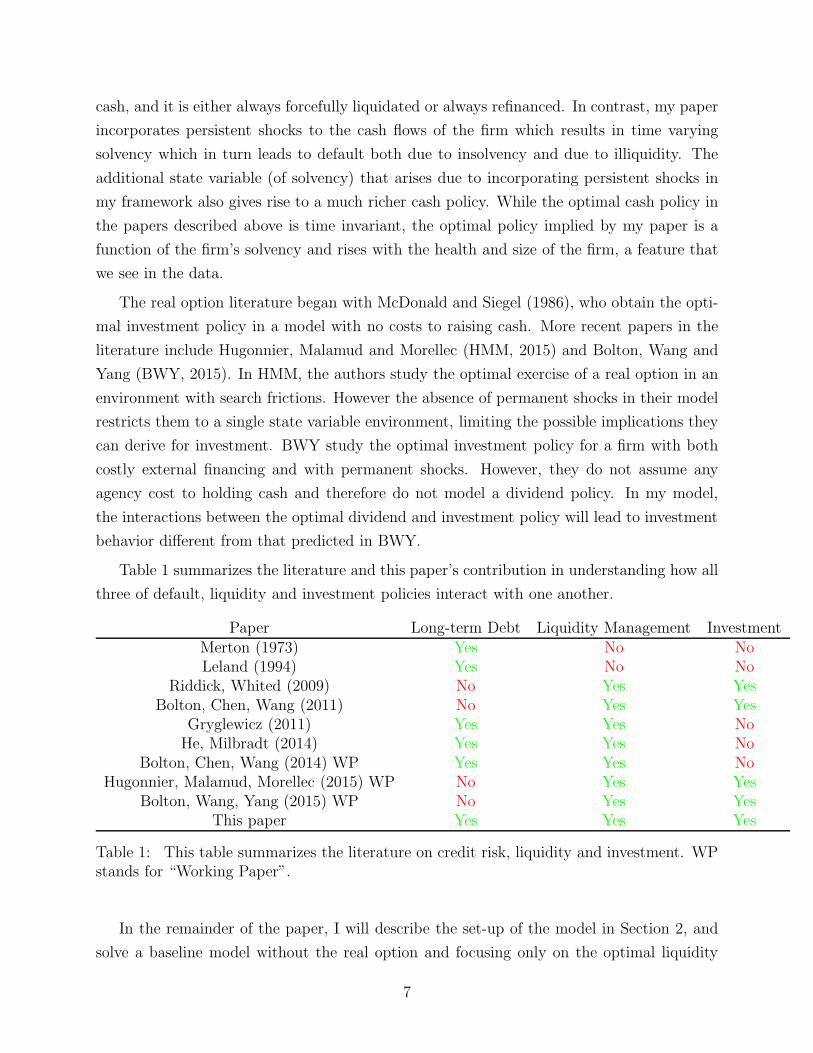
Table 1 summarizes the literature and this paper’s contribution in understanding how all

three of default, liquidity and investment policies interact with one another.

Paper Long-term Debt Liquidity Management InvestmentMerton (1973) Yes No NoLeland (1994) Yes No No

Riddick, Whited (2009) No Yes YesBolton, Chen, Wang (2011) No Yes Yes

Gryglewicz (2011) Yes Yes NoHe, Milbradt (2014) Yes Yes No

Bolton, Chen, Wang (2014) WP Yes Yes NoHugonnier, Malamud, Morellec (2015) WP No Yes Yes

Bolton, Wang, Yang (2015) WP No Yes YesThis paper Yes Yes Yes

Table 1: This table summarizes the literature on credit risk, liquidity and investment. WPstands for “Working Paper”.

In the remainder of the paper, I will describe the set-up of the model in Section 2, and

solve a baseline model without the real option and focusing only on the optimal liquidity

7

policy in Section 3. In Section 4, I solve the full model with the real option and detail the

behavior of firm investment policy in Section 5. I discuss preliminary empirical work in

Section 6 and Section 7 concludes.

2 Capital Structure and Cash Holdings:

The firm employs a stock of capital for production. It is also exposed to a productivity

process Zt which is random and which determines the earnings generated by the stock of

capital. I denote capital by X , and Xt is the level of capital stock for the firm at time t.

Earnings at time t is given by XtdZt. The productivity technology Zt evolves according to

dZt = µdt+ σdWt

where Wt is a standard Brownian Motion. Thus productivity shocks are assumed to be

random and i.i.d. µ > 0 is the drift of the productivity shock, while σ > 0 is the volatility

of the shock.

The firm’s gross cash flow (dYt) over the time increment dt is given by

dYt = XtdZt = µXtdt+ σXtdWt (1)

I assume that the revenue generating equation, 1 is risk-adjusted and holds under the

risk-neutral measure. Equity and Debt holders discount payoffs at the risk-free rate r > 0.

Long-term debt: The firm issues debt and trades off the tax benefits of debt with the

expected bankruptcy cost associated with the risk of default. I assume that debt takes the

form of a consol bond with coupon k. At every instant dt, the firm pays out an amount kdt

to creditors. I also assume that earnings after interest payment are taxed at the corporate

income tax rate τ . Therefore, the after tax cash flow generated by the firm, in time increment

dt, after paying debt is equal to (1 − τ)(dYt − kdt) = dYt − kdt, where Yt = (1 − τ)Yt and

k = (1− τ)k. I will refer to Yt as net cash flows.

Costly External Financing and the role for cash: The firm has to pay a financing

cost if it has to raise money by issuing equity from the external capital markets. If the

firm does not hold any liquidity, and if current earnings are not sufficient to pay creditors

(dYt < kdt), then the firm will have to issue equity. I assume that if the firm chooses to

raise v in liquid assets, then the cost it incurs is given by Φ(v) = γv + FC, where FC is

the fixed cost of equity financing and γ is the marginal cost of financing. I assume for the

8

rest of the paper that γ = 1. As will be seen later on, this assumption on the marginal cost

of financing simplifies the model considerably. Given the cost associated with issuing new

equity, it is always optimal for the firm to hold some cash as a buffer. Due to the continuous

time nature of the model, if the firm does not hold any cash, then it will have to pay the

external financing cost with probability 1 immediately.

The cash holdings of the firm are set by equity holders. Cash earns a return equal to

the risk free rate (r) net of a carry cost of holding cash (λc), common in dynamic agency

models. More specifically, I assume that managers can divert liquid assets in the firm to

take advantage of private benefits or invest in inefficient projects. I model the cost of these

actions in a reduced form manner as a lower rate of return earned by liquid assets. λc = 0 is

the first-best outcome. Under this benchmark, cash in the firm earns the same rate of return

as more illiquid assets, and so the firm trivially finds it optimal to hold as much cash as it

can to prevent default. As such, the firm does not pay any dividends. The more realistic

case is when λc > 0. On the one hand, cash in the firm now earns a lower rate of return than

illiquid assets. On the other hand, the firm holds liquidity for precautionary reasons to lower

the expected financing cost it may have to pay if it runs out of liquid funds. Firms therefore

manage an optimal cash policy where they trade off the liquidity benefits of maintaining a

cash reserve against the cost due to agency frictions of holding cash. Solving for this optimal

policy is a central feature of the model and affects the prices of contingent claims.

Investment: I consider two types of investment in this paper. First, the firm can invest

in a “neoclassical manner” by converting its stock of cash into capital or vice-versa. Second,

the firm can undertake “real investment” by exercising a growth option after paying a cost.

Neoclassical Investment: When modeling neoclassical investment, I assume that in-

vestors decide at time 0 a rate of expansion or contraction of the firm φ. This rate captures

how much of earnings (after paying off debt) is plowed back into capital and how much is

saved as cash or paid as dividends. The firm is hit by neoclassical investment shocks how-

ever where it can convert its stock of cash into capital (invest) or convert capital into cash

(disinvest) after paying a cost. For an additional cost, the firm may also choose to reset its

capital structure when the neoclassical shocks hit. The reset of capital structure will involve

buying back debt at par value and re-issuing a new consol bond. Additionally, the firm may

also issue equity if required.

Discussion: The way I model neoclassical investment in this paper is a combination of

how investment is modeled in , among others, DeMarzo and Fishman (2007) and Bolton,

Chen and Wang (2011, hereafter BCW). In the former paper, investment is modeled as a

decision to expand or contract the firm each period. This rate is continually set by investors

9

after paying a cost. In BCW, investment is modeled as a continuous control variable chosen

by equity holders to maximize equity value.

In this paper, I assume that the scale of the firm is fixed through time, so there is

continuous “internal investment” where the firm transforms cash into capital at a fixed rate;

however, the firm can also engage in investment of the type modeled in BCW when hit

by the neoclassical investment shocks. Therefore investment in my model only differs from

BCW in that it is sticky and not continuous. This stickiness is a key feature generating

model tractability and also leads to credit risk as the firm gets close to default. Similar to

Hennessy and Whited (2005), I also assume that if the firm wants, it can restructure debt

or issue equity when the investment shocks arrive. This reset of capital structure occurs

endogenously when the firm is not too close to default.

Real Investment: The firm is also hit by real investment shocks at which point it can

choose to exercise a growth option - paying a cost I from its cash reserves. I assume that the

firm can exercise the real option only once and only when it gets hit by the real investment

shock. Thus cash in the firm is not only used for precautionary or hedging purposes, but

also to fund investment when the shock arrives.

After exercising the growth option, the new productivity process becomes

dZt = µHdt+ σHdWt

where µH/µ = σH/σ = q > 1. Thus the growth option involves a form of “real scaling” of

the firm’s cash flow process, where the scaling does not come from an expansion in capital

stock, but instead from a higher average productivity of capital.

Valuing equity and debt: The value of equity is determined by the discounted sum of

dividend payments until the firm defaults, while debt value is given by the discounted value

of the constant coupon of the consol bond until default. At default, I assume that creditors

recover a fraction of residual firm value, and lose the rest through bankruptcy costs.

At every instant, equity holders may choose to use generated net cash flow to either pay

dividends, or save as cash. At the same time, if a real investment shock hits, they must decide

if they choose to exercise the real option or not. Similarly, if the neoclassical investment

shock hits, equity holders can decide whether to convert cash into capital, burn capital into

cash or reset firm capital structure. Equity holders can also choose when to trigger default.

Therefore, equity holders chose the optimal default, liquidity and investment policy for the

firm.

Evolution of Capital and Cash: As discussed earlier, φ is the “scale” of the firm and

10

determines the continuous rate at which generated earnings are converted back into capital.

I set λn to be the hazard rate of neoclassical investment shocks and λr to be the hazard rate

of real investment shocks. Recall that when the real shocks hit, the firm chooses to exercise

the growth option. Let τ be the (random) time of exercise of the growth option.

Then, for t < τ ,

dXt = φ [(µXt − k)dt+ σXtdWt] + ItdNt

dCt = (r−λc)Ctdt+(1−φ) [(µXt − k)dt+ σXtdWt]−ItdNt−g(It, Xt)dNt+dDivt+1t=τeEQt

In the above equations, before the real option is exercised, the change in capital in the

absence of neoclassical investment shocks is captured by the rate φ at which generated

cashflows after debt payments is converted into capital. The investment shock is modeled

as a Poisson process Nt. When the shock hits, equity holders invest It units of capital.

The change in cash holdings equals the generated earnings less the amount that is con-

verted into capital (i.e. a fraction (1 − φ) of generated earnings). When the investment

shock hits, and the firm invests It units of capital, this involves debiting this amount from

the store of cash in the firm. Also, g(It, Xt) is the investment adjustment cost. The cumu-

lative dividends paid by the firm is given by Divt. At any time, τe, the firm may also issue

external equity, raising an amount of cash EQt, paying the fixed cost Fc. Divt, EQt and τe

are endogenous and capture the dividend and equity issuance policy for the firm.

After exercising the growth option, for t > τ

dXt = φ [(µHXt − k)dt+ σHXtdWt] + ItdNt

dCt = (r−λc)Ctdt+(1−φ) [(µHXt − k)dt+ σHXtdWt]−ItdNt−g(It, Xt)dNt+dDivt+1t=τeEQt

Assumption: r = λc

I assume that cash in the firm does not earn a return and the carry cost associated with

holding cash exactly cancels the return it would otherwise earn.

Thus cash in the firm can be treated as if it “placed under a mattress”. This assumption is

made purely for analytical reasons. As will be clear in the following section, this will allow

a “dimensionality reduction” which can help to solve a two-state variable problem in closed

form.

11

3 Solving the Model - baseline case:

Initially, to show intuition, I will solve the model in the absence of any investment shocks

(real or neoclassical). Capital and cash in this baseline model evolve according to

dXt = φ [(µXt − k)dt+ σXtdWt]

dCt = (1− φ) [(µXt − k)dt+ σXtdWt] + dDivt + 1t=τeEQt

Therefore, investment is exogenous in this framework (with rate φ determined at time 0).

Costly external financing results in the presence of a non-trivial liquidity policy. Even in

the baseline model, the presence of permanent shocks to firm cash flows and the penalty

to issuing equity result in both solvency and liquidity channels of default. As discussed

earlier, existing models of structural credit risk with exogenous investment do not also model

liquidity management. An exception is Gryglewicz (2011) where the firm faces liquidity risk

and so has a dynamic cash policy, and where solvency risk arises from a dynamic average

productivity (dynamic µ). By contrast, the baseline model in my paper is more in line with

other credit risk papers in that it is the presence of permanent shocks to the firm’s capital -

rather than productivity - that results in solvency risk.

The solution of the model will consist of explicitly obtaining the prices of equity and

debt for a given level of capital, cash and liability. These prices will in turn depend on the

optimal liquidity policy and when the firm chooses to issue additional equity.

The cash policy of the firm is determined depending on whether or not the firm is in

one of two regions. On the one hand, the firm may hoard cash, when the marginal value of

holding cash in the firm exceeds 1. I term the region in which the firm hoards cash as the

hoarding region. When the marginal value of cash becomes less than or equal to 1, the firm

may distribute cash out as dividends. This region is termed the payout region. Therefore, the

firm follows an intuitive liquidity policy: It keeps hoarding cash while the marginal value of

each dollar is greater than one. This marginal value keeps decreasing as the amount of cash in

the firm increases. Finally, when the marginal value of cash exactly equals one, the firm finds

it weakly sub-optimal to keep hoarding cash, and pays out any extra cash flows as dividends.

For any amount of capital, I define the cash boundary as that level of cash above which the

firm finds it optimal to pay out dividends. Thus when cash is below the threshold implied by

the cash boundary, the precautionary benefit of cash outweighs the agency cost associated

with cash. When cash is above the threshold, the precautionary benefit of each additional

unit diminishes to the point where it is optimal to pay it out to equity holders. Such a cash

policy is common in the dynamic liquidity management literature, arising primarily due to

12

the decrease in marginal value of cash as the level of cash increases.

To fully capture the liquidity policy of the firm, it is also necessary to determine when the

firm will tap external markets to issue equity. Since the firm faces a fixed cost of financing,

it chooses to tap the market to raise equity infrequently. It will optimally raise cash only

when it runs out of liquidity. The intuition is that when the firm faces a fixed cost of issuing

equity, it will choose to delay paying these costs for as long as possible. Therefore, when the

firm runs out of cash, equity holders can perform one of two actions. Either they can choose

to issue new equity, diluting their existing stake by the total cost of equity issuance. Or they

choose to not issue new equity and, because there is no cash in the firm to pay creditors,

they are forced to liquidate.

I assume that the marginal cost of issuing equity equals 1. This means that equity holders

will keep issuing equity (and injecting cash into the firm) until the total cash level is such

that the marginal value equals 1. Since the cash boundary parametrizes the set of all points

where the marginal value of cash equals 1, it will be optimal for equity holders to raise cash

so that cash in the firm jumps up to the cash boundary upon equity issuance.

To summarize, therefore, the firm only issues equity when it runs out of cash, and issues

to an amount such that cash levels jump up to the boundary again. Otherwise, the firm

keeps hoarding cash for precautionary reasons, until cash reaches a certain threshold (as a

function of capital) at which point it starts paying dividends.

In the hoarding region, therefore, dDivt = 0, and 1t=τe = 0. Thus,

dCt = (1− φ)/φdXt (2)

Therefore, the change in cash level of the firm is proportional to the change in capital stock

in the hoarding region.

The tight link between changes in capital and cash while the firm is hoarding can be seen

in Figure 1. When the firm is hoarding cash, Equation 2 implies that the firm moves along

a straight line until it either runs out of cash or defaults. Thus, for any given value of (x, c),

the value of cash and capital at which the firm starts paying dividends is fixed. Similarly, the

value of capital at which the firm runs out of cash is also fixed. I call xu(x, c) and xℓ(x, c) to

be the unique values of capital at which the firm pays dividends or issues equity respectively.

The values of xu as a function of x and c determines the cash boundary.

I will denote xd as the threshold of capital below which equity holders trigger default due

to solvency. Note that strategic default by equity holders will only happen when cash in the

firm equals zero. To see this, assume for contradiction that the firm defaults at (x, c), where

13

Ct

Xt

C(xt)

(xu, C(xu))

(x, C)

τD

(xD, 0) (xl, 0)

(xl, C(xl))

tan−1((1− φ)/φ)

q1

q2

bA

b

B

GD

Q

Figure 1: In the above figure, if the firm’s cash and earnings are such that it is at point A, then it may only move on

the dashed line until it either hits the boundary (at point B) or runs out of cash (point G) at which point, it raises equity if it

chooses, jumping back to Q and paying a fixed cost. If it does not choose to raise equity when running out of cash, the firm

gets liquidated at G. The firm may also default due to solvency at time τD when x hits the level xD. Once the firm hits the

boundary, then it moves along the boundary if earnings shocks are positive, while slipping back into the hoarding region if the

shocks are negative.

0 < c < C(x). Then, since debt holders are senior claimants on the firm and will seize all

the cash when the firm defaults, equity holders will optimally pay out all cash as dividends

the instant before triggering default, i.e. they will set C(xd) to zero. Therefore, default will

only happen when the cash level of the firm is at zero. At this point, the payout region and

hoarding region coincide (they collapse to a single point).

This greatly simplifies the analysis when computing credit spreads, since it implies a

strategic default “region” of a single point, similar to standard credit risk models. Of course,

the firm may also have to liquidate if it runs out of cash, and this will be reflected in credit

spreads.

Together, the evolution of cash and capital in this baseline model with the default thresh-

old is shown in Figure 1.

14

Let us denote E(x, c) and Ep(x, c) as equity value in the hoarding and payout region

respectively. In the payout region, the firm pays out cash as dividends until cash levels fall

back to the cash boundary again (and equal C(x)). Thus, equity value in the payout region

is given by

Ep(x, c) = E(x, C(x)) + c− C(x)

when c > C(x).

When solving for the prices of contingent claims, I make use of two other conditions

that must hold at the cash boundary. These are the smooth pasting and supercontact

conditions. If a traded claim takes different functional forms in different regions of space,

then the smooth pasting condition equates the derivative of this traded claim at the boundary

separating these two regions. This is a condition that must hold due to no-arbitrage. In

the payout region, clearly ∂Ep(x, c)/∂c = 1. Therefore, we can impose the smooth pasting

condition to postulate that

∂E(x, c)

∂c|c=C(x) = 1 (SmoothPastingCondition)

The above condition holds for any barrier policy of cash holdings.

At the optimal barrier, we can further impose the Supercontact condition.

∂2E(x, c)

∂c2|c=C(x) = 0 (SuperContactCondition)

3.1 Valuing Equity:

I will value equity (and debt) in two stages. First, I will obtain the value of equity and debt

on the cash boundary. Next, I will obtain the value of each in the hoarding region. Finally,

I will impose an optimality condition to explicitly obtain the cash boundary.

Equity value equals the discounted sum of all dividend payments until default net of the

total amount of issuances. Similarly, debt value equals the discounted sum of all coupons

paid until default plus the expected recovery value of the firm at default.

E(x, c) = supDiv

∫ t=τD

t=0

e−rt (dDivt − dEQt) (3)

Equity value in the hoarding region E(x, c) satisfies the following Hamilton-Jacobi-Bellman

15

Equation

rE(x, c) = (µx− k)[φEx + (1− φ)Ec] +1

2σ2x2[φ2Exx+ (1− φ)2Ecc + 2φ(1− φ)Exc] (4)

The left hand side of Equation 4 is the required rate of return on equity, which just equals

the risk free rate since all investors are risk neutral and since there is no arbitrage. The first

term on the right hand side is the effect of the expected change in capital and cash on equity

value. The second and third term capture the effect of volatility on equity value.

Proposition 1a: Equity value on the boundary

Let E(x) = E(x, C(x)) denote equity value when the firm pays dividends and stops hoarding

cash. Then,

E(x) = [(1− φ)(µx− k)

r − µφ]− [

(1− φ)(µxd − k)

r − µφ](x

xd

)r2F (r2; x)

F (r2; xd)(5)

where r2 is the negative root of the quadratic equation 12φ2σ2x(x− 1) + φµx− r = 0.

F (r2; x) denotes the Kummer function, and is defined in the Appendix.

Proof: See Appendix

We can see from the above formulation that equity value on the boundary while holding

cash is the expected future cash flows from the firm net of liabilities minus a term capturing

the expected losses from default. On the cash boundary at which the firm starts paying

dividends, the smooth pasting and supercontact conditions together imply that the value of

equity equals its value in the first-best case with no external financing costs and hence no

role for cash. This is common in dynamic models of cash holdings.

The intuition is that in a frictionless world, the marginal value of cash always equals 1

since the firm always pays out any cash to shareholders as dividends or raises it costlessly

(which can be treated as a form of negative dividend). Since the marginal value is constant,

it is not sensitive to any stock of cash in the firm, i.e. Ecc = 0. Therefore, at the optimal

barrier policy of cash holdings, both the marginal value of cash and the sensitivity of this

marginal value are identical to those in the first-best case. The cost of financial frictions is

captured by the amount of cash the firm needs to hold to deliver what would otherwise be

the first-best equity value.

The above equation also indicates that equity value on the cash boundary is increasing

both in the drift (µ) and in the volatility (σ) of the productivity process. The positive

effect of σ on equity value is common in standard models of credit risk with endogenous

16

default. Equity is like an option on firm value and so benefits from increased volatility. In

a model with costly financing, however, it is uncertain whether or not equity value benefits

from volatility. While equity value on the boundary increases in volatility, I will show later

that the cash boundary itself is pushed out with increased volatility and so the cost of

financial frictions increases. For most parameter values, it turns out that this increased cost

of financial constraints due to high volatility outweighs the real-option benefits.

Proposition 1b: Equity value in the hoarding region

In the hoarding region, equity value depends on whether the firm chooses to raise cash when

it runs out of liquidity. It is given by

E(x, c) =

q1(x, c)E(xu) + q2(x, c)(

E(xl)− Fc − C(xl))

, if E(xl) > Fc + C(xl)

q1(x, c)E(xu), otherwise.(6)

where xu(x, c) is the value of capital at which the firm hits the cash boundary and starts

paying dividends (refer Figure 1), while xℓ = x− cφ/(1− φ) is the level of capital at which

the firm either chooses to raise external financing by issuing equity or chooses to liquidate.

The values of q1(x, c) and q2(x, c) are listed in the appendix.

We can interpret q1(x, C) as the value of a security that pays $1 if the firm, starting at

A, reaches B before reaching G.

q2(x, C) is the value of a security that pays $1 if the firm, starting at A, reaches G before

reaching B.

Proof: See Appendix

The above result is intuitive. When the firm is hoarding cash, it does not pay dividends,

and so no cash flow accrues to equity holders in this region. Equity only starts paying

dividends when cash levels increase to the point of reaching the cash boundary.

q1(x, c) is the value of a traded financial claim that pays $1 conditional on x reaching xu

before xℓ if the current capital and cash levels of the firm are x and c respectively. Note that

q1(xu, C(xu)) = 1, and q1(xℓ, 0) = 0. Similarly, q2(x, c) is the value of a claim that pays $1

conditional on x reaching xℓ before xu.

Since equity claims only start paying off when the firm starts paying dividends, equity

value in the hoarding region is the discounted sum of equity value at xu and xℓ. If the firm

decides to issue equity after it runs out of cash, it raises enough equity to jump back to

the cash boundary at xℓ. Since I assume that the marginal cost of equity financing equals

1, it is optimal for equity holders to inject liquidity into the firm while the marginal value

of liquidity is greater than 1. This means that equity holders issue equity until there is a

17

sufficient level of cash in the firm to start paying dividends again.

The value of equity at a capital level of xℓ when the firm runs out of cash and is about

to issue new claims therefore equals E(xℓ)− C(xℓ)− Fc. This reflects the dilution of equity

value by the amount of cash raised (C(xℓ)) and the external financing cost (Fc) respectively.

In addition, the firm chooses to raise equity only when equity value conditional on the

optimal issuance policy exceeds equity value at default. Since equity value equals 0 at

default, the firm chooses to raise external equity only for those levels of capital xℓ such that

E(xℓ)− C(xℓ)− Fc > 0.

This implies an equity issuance threshold of capital x∗ℓ such that E(x∗

ℓ)− C(x∗ℓ)−Fc = 0.

The firm chooses to issue equity if xℓ > x∗ℓ and chooses to default if xℓ < x∗

ℓ .

3.2 Valuing Debt:

Now we turn to valuing debt. In the model debt takes the form of a simple consol bond

paying coupon k. Debt holders are entitled to this constant stream of coupon payments until

the firm defaults. I assume that debt holders also seize a portion α of the unlevered firm

after bankruptcy. The term (1 − α) is therefore bankruptcy costs foregone by both equity

and debt holders. We can again obtain debt value in the hoarding region and the payout

region. I call Bp(x, c) and (respt. B(x, c)) to be the debt value in the payout region (and

respt. the hoarding region) when capital level is x and cash level is c.

In the payout region, by definition cash is disgorged by equity holders and paid out as

dividends until cash level falls back to the boundary again. Since all cash paid out only

accrues to equity holders, debt value is unaffected when the firm jumps from the payout

region to the hoarding region, i.e.

Bp(x, c) = B(x, C(x))

By the Ito Formula, debt in the hoarding region follows the HJB equation

rB(x, c) = k + (µx− k)[φBx + (1− φ)Bc] +1

2σ2x2[φ2Bxx + (1− φ)2Bcc + 2φ(1− φ)Bxc]

The intuition is similar to that for equity. The left hand side is the required rate of return for

debt, which is just the risk free rate by no-arbitrage and risk neutrality. The right hand side

is the expected rate of return decomposed into the flow payment to creditors, the marginal

effects of capital, cash and the second order volatility effects.

18

I obtain the value of debt in several steps. I first obtain the value of a claim that pays 1

dollar when the firm defaults. This helps establish the present value at default of the residual

claim on the firm for creditors. This also gives us the present value of all coupons paid out

to creditors until default.

Since debt is a traded claim, by no-arbitrage it has to satisfy (like Equity) a smooth-

pasting condition with respect to cash, i.e. ∂B(x, c)/∂c|c=C(x) = ∂Bp(x, c)/∂c|c=C(x).

But since ∂Bp(x, c)/∂c = 0, the above condition implies

∂B(x, c)

∂c|c=C(x) = 0

Note that since the cash boundary is optimally chosen by equity holders (and not by creditor),

the supercontact condition does not hold. It is still possible, however, to obtain closed-form

solutions for the value of debt.

The value of debt is given by

Bt = E

∫ τD

t

e−r(s−t)kds+ αE(e−r(τD−t)VB(xτD))

This can be simplified as

Bt =k

r(1− Ee−r(τD−t)) + αE(e−r(τD−t)VB(xτD)) =

k

r(1− vt(x, C)) + αE(e−r(τD−t)VB(xτD))

where vt(x, C) is an Arrow-Debreu claim to default, i.e. is the value of a security that pays

$1 when default occurs.

The above equations reflect the fact that debt holders receive constant payment kdt at

every unit of time dt until the firm defaults which is at some random time τD, upon which

they claim a fraction α of the unlevered value of the firm, VB. The unlevered value of the

firm is a function of the capital level at which the firm defaults, xτD . This is a random

quantity also.

Proposition 2a: Debt value on the boundary is given by

−k

r[q1c + q2c] + q1cB(x)− x′

u(xℓ)B′(x) + q2cf(xℓ) = 0 ; lim

x→∞B(x) = k/r

where f(xℓ) = B(xℓ) if the firm does not default when running out of cash and f(xℓ) =

αVB(xℓ) otherwise.

Proof: See Appendix

19

The intuition for the above equation is that the marginal value of cash on debt value at

the cash boundary equals zero. This is because, at the cash boundary, any increase in cash

level for the firm will be paid out to equity holders and not stored in the firm, leaving credit

risk unaffected. The above equation is then just the smooth-pasting condition for debt on

the dividend boundary.

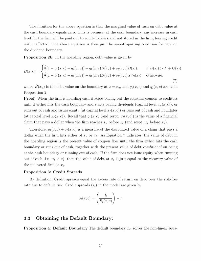
Proposition 2b: In the hoarding region, debt value is given by

B(x, c) =

kr(1− q1(x, c)− q2(x, c)) + q1(x, c)B(xu) + q2(x, c)B(xl), if E(xl) > F + C(xl)

kr(1− q1(x, c)− q2(x, c)) + q1(x, c)B(xu) + q2(x, c)αVB(xℓ), otherwise.

(7)

where B(xu) is the debt value on the boundary at x = xu, and q1(x, c) and q2(x, c) are as in

Proposition 2

Proof: When the firm is hoarding cash it keeps paying out the constant coupon to creditors

until it either hits the cash boundary and starts paying dividends (capital level xu(x, c)), or

runs out of cash and issues equity (at capital level xℓ(x, c)) or runs out of cash and liquidates

(at capital level xℓ(x, c)). Recall that q1(x, c) (and respt. q2(x, c)) is the value of a financial

claim that pays a dollar when the firm reaches xu before xℓ (and respt. xℓ before xu).

Therefore, q1(x, c) + q2(x, c) is a measure of the discounted value of a claim that pays a

dollar when the firm hits either of xu or xℓ. As Equation 7 indicates, the value of debt in

the hoarding region is the present value of coupon flow until the firm either hits the cash

boundary or runs out of cash, together with the present value of debt conditional on being

at the cash boundary or running out of cash. If the firm does not issue equity when running

out of cash, i.e. xℓ < x∗ℓ , then the value of debt at xℓ is just equal to the recovery value of

the unlevered firm at xℓ.

Proposition 3: Credit Spreads

By definition, Credit spreads equal the excess rate of return on debt over the risk-free

rate due to default risk. Credit spreads (st) in the model are given by

st(x, c) =

(

k

Bt(x, c)

)

− r

3.3 Obtaining the Default Boundary:

Proposition 4: Default Boundary The default boundary xD solves the non-linear equa-

20

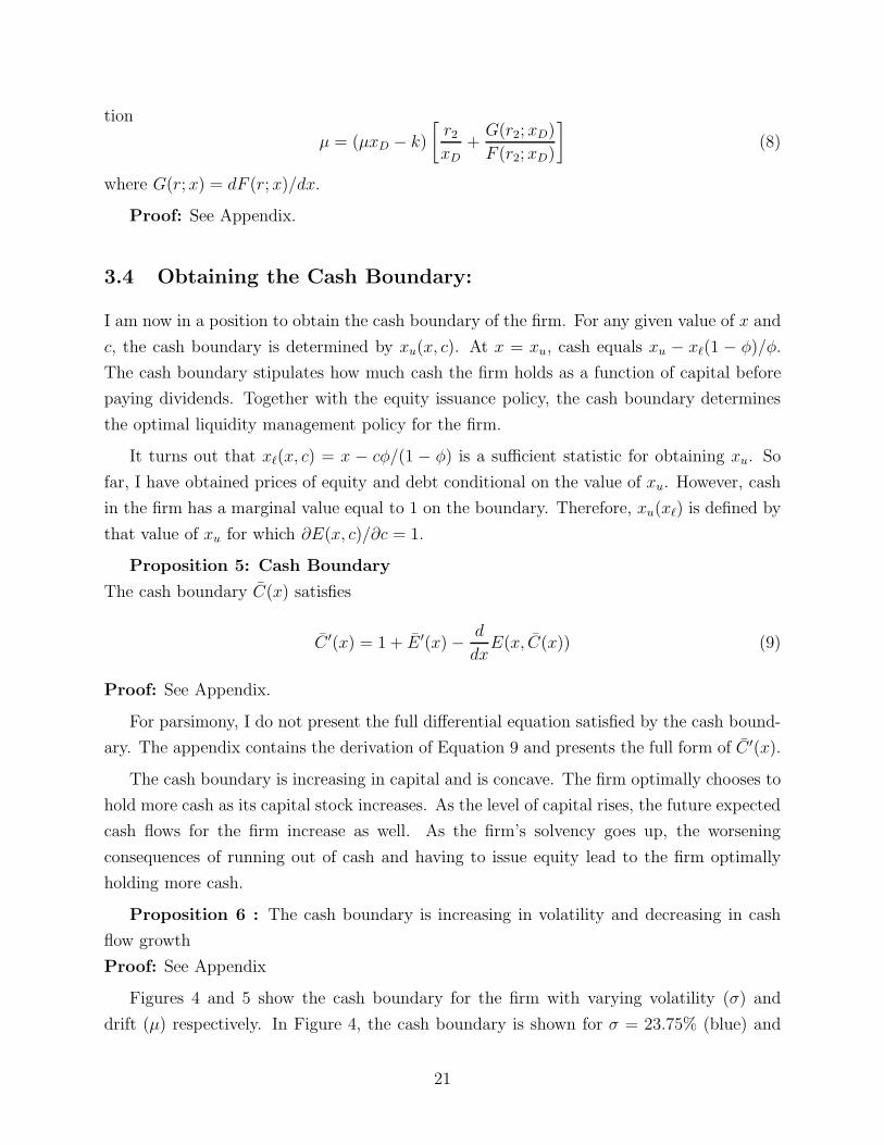
tion

µ = (µxD − k)

[

r2xD

+G(r2; xD)

F (r2; xD)

]

(8)

where G(r; x) = dF (r; x)/dx.

Proof: See Appendix.

3.4 Obtaining the Cash Boundary:

I am now in a position to obtain the cash boundary of the firm. For any given value of x and

c, the cash boundary is determined by xu(x, c). At x = xu, cash equals xu − xℓ(1 − φ)/φ.

The cash boundary stipulates how much cash the firm holds as a function of capital before

paying dividends. Together with the equity issuance policy, the cash boundary determines

the optimal liquidity management policy for the firm.

It turns out that xℓ(x, c) = x − cφ/(1 − φ) is a sufficient statistic for obtaining xu. So

far, I have obtained prices of equity and debt conditional on the value of xu. However, cash

in the firm has a marginal value equal to 1 on the boundary. Therefore, xu(xℓ) is defined by

that value of xu for which ∂E(x, c)/∂c = 1.

Proposition 5: Cash Boundary

The cash boundary C(x) satisfies

C ′(x) = 1 + E ′(x)−d

dxE(x, C(x)) (9)

Proof: See Appendix.

For parsimony, I do not present the full differential equation satisfied by the cash bound-

ary. The appendix contains the derivation of Equation 9 and presents the full form of C ′(x).

The cash boundary is increasing in capital and is concave. The firm optimally chooses to

hold more cash as its capital stock increases. As the level of capital rises, the future expected

cash flows for the firm increase as well. As the firm’s solvency goes up, the worsening

consequences of running out of cash and having to issue equity lead to the firm optimally

holding more cash.

Proposition 6 : The cash boundary is increasing in volatility and decreasing in cash

flow growth

Proof: See Appendix

Figures 4 and 5 show the cash boundary for the firm with varying volatility (σ) and

drift (µ) respectively. In Figure 4, the cash boundary is shown for σ = 23.75% (blue) and

21

σ = 19% (red) respectively. Drift µ is fixed at 5%, while k is set to 10, r is set to 6% and φ

set to 0.5. We see from the figure that for all values of capital, the amount of cash held by

the firm when volatility is higher exceeds that held when risk is lower. For any given level

of capital and cash, an increase in volatility increases the probability that the firm will run

out of liquidity and have to incur the cost of equity dilution. This increase in probability

lowers the “effective” value of equity and leads to equity holders choosing to hold more cash

for precautionary reasons.

Further, due to limited liability of equity, the default threshold of capital falls when

volatility increases. Equity holders are more likely to continue operating the firm at low

levels of capital when volatility is high hoping for a large increase in earnings.

In Figure 5, the cash boundary is shown for µ = 4% (blue) and µ = 5% (red) respectively.

Volatility σ is fixed at 19%, while k is set to 10, r is set to 6% and φ set to 0.5. We see that

for low values of capital, a firm with higher earnings growth holds a higher amount of cash.

This reverses however as capital stock becomes high. The intuition is as follows. The default

boundary is a decreasing function of cash flow growth rate, µ, since equity holders are willing

to continue running the firm with low capital stock if they believe future earnings are going

to be high. Therefore, for low values of capital, the firm with low earnings growth is much

closer to default than the firm with high growth rate. Since the solvency of the low-growth

firm is so much lower than the solvency of the high-growth firm, the costs of losing out on

future earnings due to illiquidity are also lower when µ is low. The low costs of illiquidity in

turn imply a lower level of cash employed by low-growth firms as a hedge.

On the other hand, as capital stock increases, the stock of cash held by the firm with

high growth is lower. The intuition is that at high levels of capital, the firm with high

productivity is much less likely to run out of cash and require external financing. This

mitigates the incentive to hold cash for precautionary purposes and the firm is more likely

to pay dividends.

In the model, the level of capital (relative to the default threshold) at which low growth

firms start holding more cash than high growth firms is quite low. For instance, in Figure

5, the low growth firm has a leverage of more than 50% (making it a BB-rated firm) when

it starts holding more cash.

3.5 Liquidity and Solvency Components of default:

Costly external financing results in a cash policy for the firm and gives rise to liquidity

risk. The stock of capital determines future earnings of the firm and is a measure of firm

22

solvency. In a frictionless world without costly external financing, there is no liquidity risk

and all credit risk arises through solvency. Thus I determine the liquidity component of

credit risk by comparing the credit spread obtained in my model with the credit spread

under a first-best framework with no cash.

Call st,FB to be the credit spread under the first-best environment. Then,

st,FB(x, c) =

(

k

Bt,FB(x, c)

)

− r

where Bt,FB(x, c) is the first-best value of debt and is given byBt,FB(x, c) = (x/xD)r2F (r2; x)/F (r2, xD).

The liquidity component of default is given by

ℓ(x, c) = 1−st,FB(x, c)

st(x, c)

ℓx,c captures the relative increase in credit risk compared to the first-best case that arises

due to liquidity.

23

4 Investment as a Real Option:

4.1 Model

In this section, I generalize the baseline model by incorporating real investment. In partic-

ular, the firm is hit by a sequence of real investment opportunity shocks. Whenever each

shock hits, the firm can decide whether it wants to exercise a real option. When the firm does

decide to exercise, it must pay a cost I, but then has access to a better project (captured by

better average productivity) and better set of cash flows. I assume that the firm only has

access to a single real option and that if it invests this option once, it is not hit by any more

investment shocks, and so cannot invest again. I will primarily consider the case where the

cost I scales with capital, i.e. I = i×x, where i is constant, but I will also consider the case

where I is constant when discussing comparative statics.

Prior to investment, productivity Zt is random and follows the process dZt = µdt+σdWt

where Wt is a standard Brownian Motion. After investment, the firm has access to a new

productivity process ZHt , which follows dZH

t = µHdt+σHdWt, where µH/µ = σH/σ = q > 1.

Therefore, earnings scale up by the factor q when exercising the real option. This scaling

arises from an increase in the average productivity rather than a change in the amount of

capital.

The choice for the firm to invest - conditional on being hit by a shock - depends on the

stock of cash and capital it maintains. Investing involves a direct cost I to exercise the real

option, but also incorporates an indirect cost captured by the increased probability that the

firm will run out of cash after investing and have to either default or issue new equity. This

indirect cost depends on the stock of cash after investing, which in turn depends on the

amount of cash in the firm prior to investment. The effective cost of investment therefore

depends not only on the cost I, but also on σH and µH , the volatility and growth of cash

flows after investing. A high µH decreases the indirect cost of investment by lowering the

likelihood of running out of cash. The effect of σH on the indirect cost of investment is more

interesting. On the one hand, equity holders are protected by limited liability and so an

increase in σH has a positive effect on equity due to the standard effect of volatility on a

call option. On the other hand, an increase in σH has a negative effect on equity since it

increases the probability of running out of liquidity and incurring the costs of issuing equity.

The overall effect of a change in σH on equity value depends on which of the two effects

described above is stronger. When the amount of cash in the firm is high, the firm is

effectively unconstrained financially. The positive effect will dominate and equity value will

rise with volatility. When the amount of cash in the firm is low, the firm is heavily constrained

24

financially and the negative effect dominates, resulting in a large indirect cost of investment.

Evolution of capital and cash:

Cash flows in time dt change from XtdZt prior to investment to XtdZHt after investment.

Since debt is a consol bond with coupon k, the firm has to debit an amount kdt each period

from its cash flows. Therefore, the incremental cash flow (dYt) for a firm with capital stock

xt after paying debt satisfies

dYt = 1t<τ [(µXt − k)dt+ σXtdWt] + 1t>τ [(µHXt − k)dt+ σHXtdWt]

As before, the firm also maintains a “scale” of φ, which is the rate at which the firm

plows back its earnings into capital. This scale holds both before and after exercising the

real option. In this section, I assume that there are no neoclassical investment shocks,

and so I do not assume any other cash-capital conversions. Incorporating the neoclassical

investment shocks does not change the economics of the model.

Therefore, in the presence of real investment shocks, capital (Xt) and cash (Ct) evolve

according to the following process, where τ is the random time of exercise of the real option:

dXt = 1t<τ (φ [(µXt − k)dt+ σXtdWt]) + 1t≥τ (φ [(µHXt − k)dt + σHXtdWt])

dCt = 1t<τ ((1− φ) [(µHXt − k)dt+ σXtdWt]) + 1t≥τ ((1− φ) [(µHXt − k)dt+ σHXtdWt])− I1t=τ

− dDivt (10)

Equation 10 indicates that capital is invested at the plow-back rate φ both before and

after exercising the real option. The remainder of earnings (after paying creditors) goes

towards either buffering the firm’s cash stock or paying dividends. At the time of exercise of

the real option, the firm pays an exercise cost I out of its cash reserves. I assume that the

firm does not issue equity when exercising the real option.

Note that the optimal liquidity management policy of the firm will differ depending on

whether or not the productivity process generating cash flows is Z or ZH . The increased

growth and volatility of the firm after exercising the growth option will generate a different

optimal cash and dividend policy.

Figure 2 indicates how cash and capital evolve in the model with the real option. There

are two separate cash boundaries determined by whether or not the firm has exercised its

real option. Upon exercise, cash in the firm depletes by an amount I (with capital stock

remaining unchanged).

25

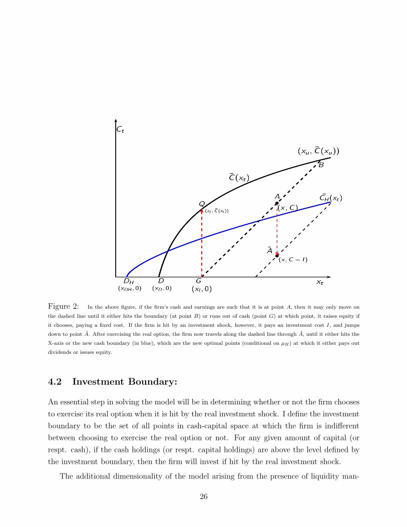
Figure 2: In the above figure, if the firm’s cash and earnings are such that it is at point A, then it may only move on

the dashed line until it either hits the boundary (at point B) or runs out of cash (point G) at which point, it raises equity if

it chooses, paying a fixed cost. If the firm is hit by an investment shock, however, it pays an investment cost I, and jumps

down to point A. After exercising the real option, the firm now travels along the dashed line through A, until it either hits the

X-axis or the new cash boundary (in blue), which are the new optimal points (conditional on µH ) at which it either pays out

dividends or issues equity.

4.2 Investment Boundary:

An essential step in solving the model will be in determining whether or not the firm chooses

to exercise its real option when it is hit by the real investment shock. I define the investment

boundary to be the set of all points in cash-capital space at which the firm is indifferent

between choosing to exercise the real option or not. For any given amount of capital (or

respt. cash), if the cash holdings (or respt. capital holdings) are above the level defined by

the investment boundary, then the firm will invest if hit by the real investment shock.

The additional dimensionality of the model arising from the presence of liquidity man-

26

agement implies an investment boundary that is far richer than that in standard real option

models, where capital is the only state variable since there is no role for cash. The investment

boundary is this framework collapses to a point and is just the threshold of capital above

which the firm invests. By contrast, in this model, the investment boundary is a function

both of the stock of capital and the stock of cash at the time of investment. I denote S to

be the set of all points in cash-capital space at which the firm does not invest (by exercising

the real option) if hit by the shock (see Fig 3) . Similarly, SI is the set of points at which

the firm does invest if it has the opportunity to do so. The investment boundary therefore

partitions the hoarding region cash-capital space into S and SI . I denote the investment

boundary function by I, and so I(x) is the investment boundary as a function of capital x. In

particular, if a firm has capital level x and cash level c < C(x) and is hit by a real investment

shock, then it is indifferent between investing and not investing if c = I(x). Note also that

I only define the investment boundary for those values of capital x for which I(x) < C(x).

Heuristically, the reason is that if c > C(x), the firm immediately pays dividends dropping

cash level down to c = C(x), and so the probability that the firm is in the payout region

and paying dividends while hit by the investment shock is zero.

Therefore, the firm is never in a position to decide to invest if liquidity levels are above

the cash boundary, and so I only define I(x) for those values of capital at which the firm will

have to choose (with non-zero probability) whether to invest or not, i.e. I(x) is only defined

for x in the hoarding region. I(x) and C(x) are determined jointly. In subsequent sections,

I will go into more detail how changes in various parameters of the model have implications

for both the investment boundary (I) and the dividend boundary (C).

The above arguments lead us to the following lemma.

Lemma1:

Let x∗ = infx x ∈ SI . Then I(x) = C(x).

Proof: See Appendix.

The above Lemma states that the cash and the investment boundaries intersect at a

particular threshold of capital, and that this is the minimal level of capital at which the

firm ever invests. If capital is below this threshold, then it becomes optimal for the firm to

start paying dividends before storing cash to the sufficient level at which it can start funding

investment. Therefore, cash is used only for precautionary motives when x < x∗, but is used

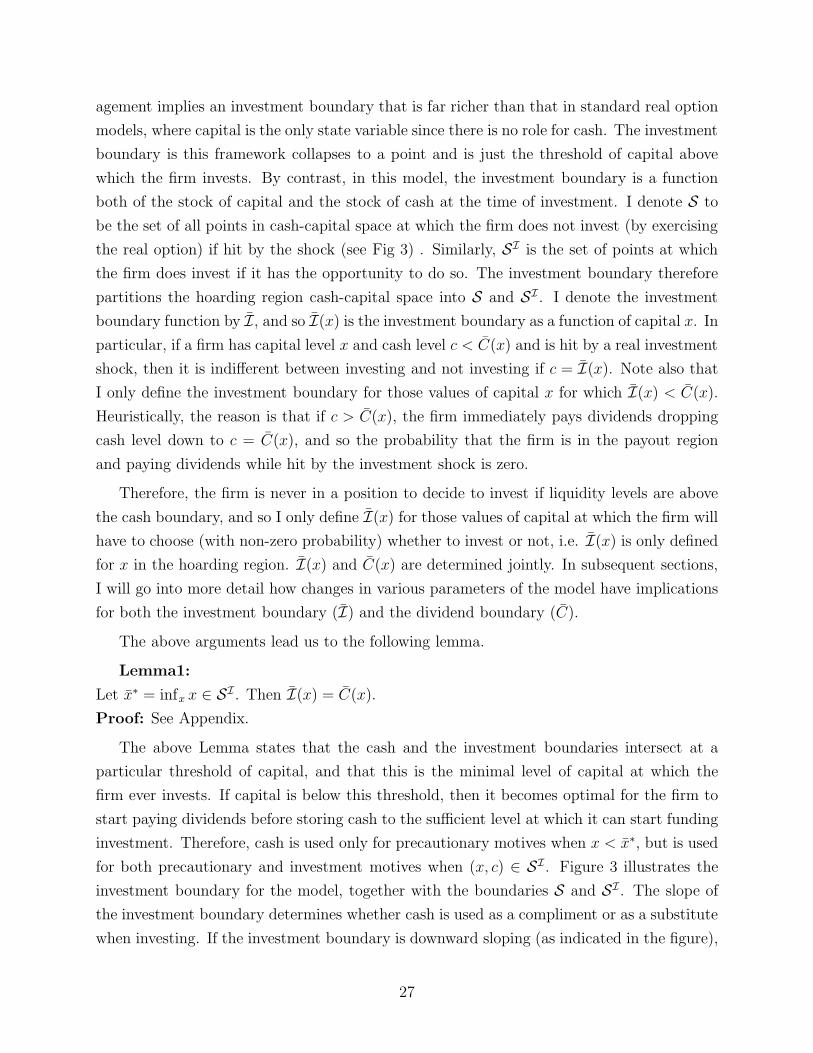
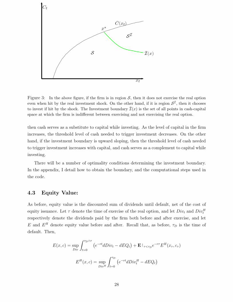
for both precautionary and investment motives when (x, c) ∈ SI . Figure 3 illustrates the

investment boundary for the model, together with the boundaries S and SI . The slope of

the investment boundary determines whether cash is used as a compliment or as a substitute

when investing. If the investment boundary is downward sloping (as indicated in the figure),

27

Ct

xt

C(xt)

S

SI

x∗

I(x)

Figure 3: In the above figure, if the firm is in region S, then it does not exercise the real option

even when hit by the real investment shock. On the other hand, if it is region SI , then it chooses

to invest if hit by the shock. The Investment boundary I(x) is the set of all points in cash-capital

space at which the firm is indifferent between exercising and not exercising the real option.

then cash serves as a substitute to capital while investing. As the level of capital in the firm

increases, the threshold level of cash needed to trigger investment decreases. On the other

hand, if the investment boundary is upward sloping, then the threshold level of cash needed

to trigger investment increases with capital, and cash serves as a complement to capital while

investing.

There will be a number of optimality conditions determining the investment boundary.

In the appendix, I detail how to obtain the boundary, and the computational steps used in

the code.

4.3 Equity Value:

As before, equity value is the discounted sum of dividends until default, net of the cost of

equity issuance. Let τ denote the time of exercise of the real option, and let Divt and DivHtrespectively denote the dividends paid by the firm both before and after exercise, and let

E and EH denote equity value before and after. Recall that, as before, τD is the time of

default. Then,

E(x, c) = supDiv

∫ τD∧τ

t=0

(

e−rtdDivt − dEQt

)

+ E1τ<τDe−rτEH(xτ , cτ )

EH(x, c) = supDivH

∫ τD

t=0

(

e−rtdDivHt − dEQt

)

28

Equity value prior to investment is the discounted sum of dividends paid to share holders net

of equity issuance costs before the first of either real investment or default. After investing,

equity value is again the sum total of all dividends - this time determined by another liquidity

management policy - until default.

By the Ito formula, we can show that equity value before investment will follow the

PDE(where subscripts denote partial derivatives)

rE = LE + λ(

EH(x, c − I)− E(x, c)) 1(x,c)∈SI ; rEH = LHEH (11)

where L and LH denote the infinitesimal generators

L = (µx− k)

(

φ∂

∂x+ (1− φ)

∂

∂c

)

+1

2σ2x2

(

φ2 ∂2

∂x2+ (1− φ)2

∂2

∂c2+ 2φ(1− φ)

∂2

∂x∂c

)

LH = (µHx− k)

(

φ∂

∂x+ (1− φ)

∂

∂c

)

+1

2σ2Hx

2

(

φ2 ∂2

∂x2+ (1− φ)2

∂2

∂c2+ 2φ(1− φ)

∂2

∂x∂c

)

Recall that we use the variables xu and xℓ to denote the levels of capital at which the

firm respectively pays dividends or raises equity/defaults. Further, if xu > x∗, then there is

a threshold value of capital (x∗, c∗) where x∗ ∈ (xℓ, xu) such that c∗ = I(x∗). Then, the firm

will choose to invest of hit by the real investment shock and if x > x∗. It will not invest

otherwise. Equity value in the hoarding region will depend on whether xu > x∗ or not.

If xu > x∗ , then the firm is in region S if x < x∗, and is in region SI otherwise. If

xu < x∗, then the firm is always in region S.

The following proposition derives the value of equity, depending on whether the firm is

in region S or SI .

Proposition 7:

Equity value in the presence of real investment shocks is given by

E(x, c) =

{

q1(x, c)E(x∗, c∗) + q2(x, c)(

E(xℓ)− C(xℓ)− Fc

)

for xu > x∗ and x < x∗

q1(x, c)E(xu) + q2(x, c)(

E(xℓ)− C(xℓ)− Fc

)

for xu < x∗

E(x, c) = q1λ(x, c)Eλ(xu) + q2λ(x, c)E(x∗, c∗) + λEp(x, c) for xu > x∗ and x > x∗

where Ep(x, c), and the expressions for q1, q2, q1λ and q2λ is given in the appendix.

We can see that the value of equity is determined by whether the firm chooses to exercise

the real option if it is hit by the investment shock. If it does not choose to exercise, it is

in region S and we have one of two cases. Either the firm starts paying dividends before

29

moving to region SI , in which case xu < x∗, or the firm transitions to SI before reaching

xu, in which case xu < x∗.

In the first case, equity value is similar to that in the baseline model with no investment.

When the firm is in the hoarding region, it never invests before hitting xu, and so q1(x, c)

and q2(x, c) can be interpreted as the prices of securities that pay a dollar when the firm hits

xu and xℓ respectively.

In the second case, equity holders still do not invest if hit by investment shocks, but

transition into region SI after crossing the capital threshold x∗. Equity value is again given

by the weighted sum of equity value at x∗ and equity value at xℓ, where the firm runs out

of cash and starts issuing equity. The weights q1 and q2 are again equal to the prices of

securities that pay a dollar when the firm hits x∗ and xℓ respectively.

When the firm is in region SI , it does invest when hit by the shock, as indicated in

equation 11. Equity value in this region is therefore determined also by the likelihood

of investment and by the value of equity after investment. q1λ and q2λ are the values of

securities that pay a dollar when the firm reaches xu or x∗ conditional on no real investment

taking place. Ep(x, c) is the additional value to shareholders for having the opportunity to

invest. Ep(x, c) will depend on µH and σH which determine the earnings for the firm after

investment. The expression for Ep is detailed in the appendix.

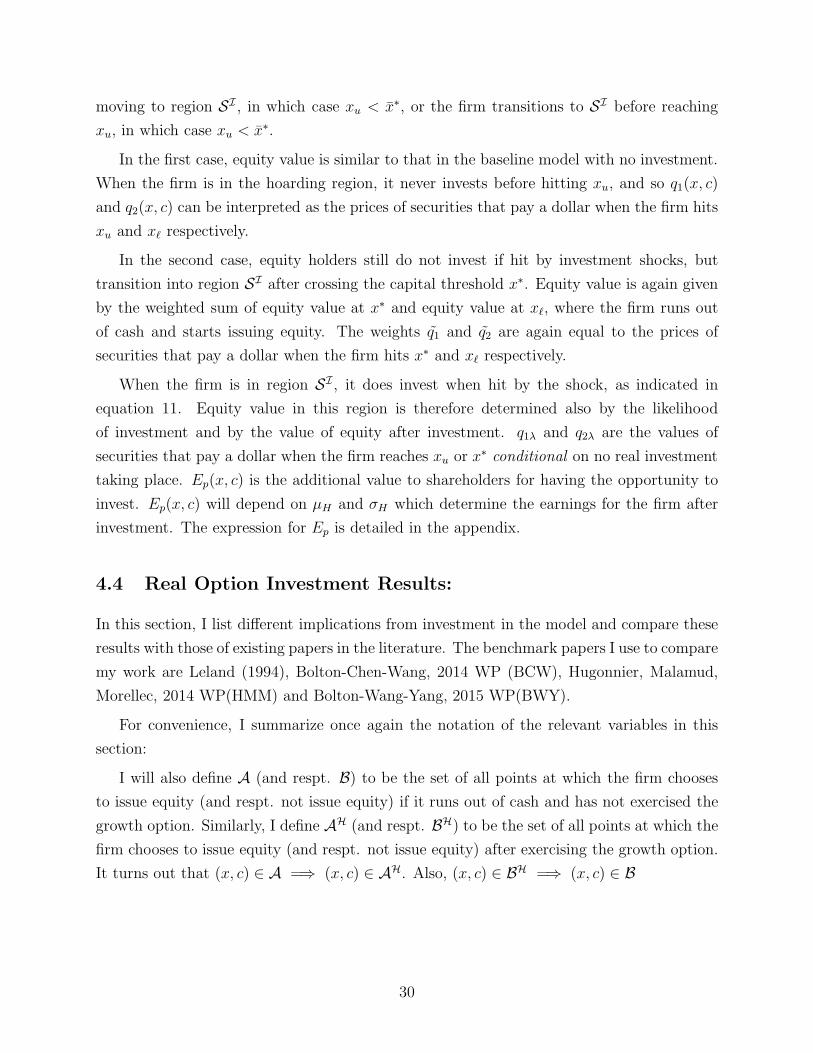
4.4 Real Option Investment Results:

In this section, I list different implications from investment in the model and compare these

results with those of existing papers in the literature. The benchmark papers I use to compare

my work are Leland (1994), Bolton-Chen-Wang, 2014 WP (BCW), Hugonnier, Malamud,

Morellec, 2014 WP(HMM) and Bolton-Wang-Yang, 2015 WP(BWY).

For convenience, I summarize once again the notation of the relevant variables in this

section:

I will also define A (and respt. B) to be the set of all points at which the firm chooses

to issue equity (and respt. not issue equity) if it runs out of cash and has not exercised the

growth option. Similarly, I define AH (and respt. BH) to be the set of all points at which the

firm chooses to issue equity (and respt. not issue equity) after exercising the growth option.

It turns out that (x, c) ∈ A =⇒ (x, c) ∈ AH. Also, (x, c) ∈ BH =⇒ (x, c) ∈ B

30

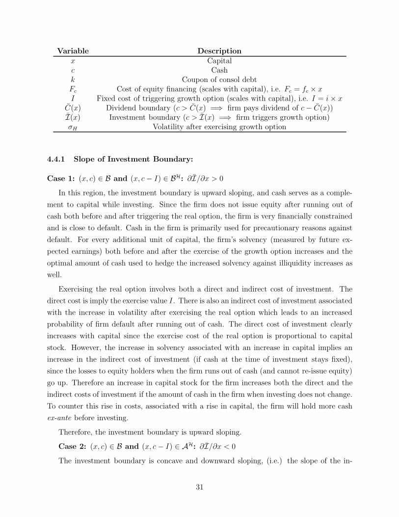
Variable Description

x Capitalc Cashk Coupon of consol debtFc Cost of equity financing (scales with capital), i.e. Fc = fc × xI Fixed cost of triggering growth option (scales with capital), i.e. I = i× x

C(x) Dividend boundary (c > C(x) =⇒ firm pays dividend of c− C(x))I(x) Investment boundary (c > I(x) =⇒ firm triggers growth option)σH Volatility after exercising growth option

4.4.1 Slope of Investment Boundary:

Case 1: (x, c) ∈ B and (x, c− I) ∈ BH: ∂I/∂x > 0

In this region, the investment boundary is upward sloping, and cash serves as a comple-

ment to capital while investing. Since the firm does not issue equity after running out of

cash both before and after triggering the real option, the firm is very financially constrained

and is close to default. Cash in the firm is primarily used for precautionary reasons against

default. For every additional unit of capital, the firm’s solvency (measured by future ex-

pected earnings) both before and after the exercise of the growth option increases and the

optimal amount of cash used to hedge the increased solvency against illiquidity increases as

well.

Exercising the real option involves both a direct and indirect cost of investment. The

direct cost is imply the exercise value I. There is also an indirect cost of investment associated

with the increase in volatility after exercising the real option which leads to an increased

probability of firm default after running out of cash. The direct cost of investment clearly

increases with capital since the exercise cost of the real option is proportional to capital

stock. However, the increase in solvency associated with an increase in capital implies an

increase in the indirect cost of investment (if cash at the time of investment stays fixed),

since the losses to equity holders when the firm runs out of cash (and cannot re-issue equity)

go up. Therefore an increase in capital stock for the firm increases both the direct and the

indirect costs of investment if the amount of cash in the firm when investing does not change.

To counter this rise in costs, associated with a rise in capital, the firm will hold more cash

ex-ante before investing.

Therefore, the investment boundary is upward sloping.

Case 2: (x, c) ∈ B and (x, c− I) ∈ AH: ∂I/∂x < 0

The investment boundary is concave and downward sloping, (i.e.) the slope of the in-

31

vestment boundary becomes more negative and cash level required to trigger investment

decreases with capital. In this region, the firm gets liquidated if it runs out of cash without

exercising the growth option, but issues equity and continues running if it runs out of cash

after exercising the growth option.

The firm endogenously chooses to raise external finance after exercising the growth option.

This means that an increase in capital stock increases the value of the firm through two

separate channels. On the one hand, if the firm is hit by a sequence of positive productivity

shocks, the increased stock of capital increases the total earnings of the firm and makes it

more likely that the firm will start paying dividends. On the other hand, if the firm is hit by

a sequence of negative productivity shocks, the constant plow-back policy of the firm implies

that the stock of capital left in the firm when it issues equity also increases, i.e. the solvency

increases when it runs out of cash.

We can now compare the value of cash in a firm if it does or does not raise external

financing when running out of liquidity. If the firm is constrained enough to not issue equity,

then an increase in capital stock in the firm increases the value of cash since the consequences

to equity holders of running out of liquidity and having to default are higher. But if the

firm does issue equity, then an increase in capital stock still increases the value of liquidity,

but the positive benefit of cash is mitigated somewhat by the decreased likelihood to equity

holders of issuing equity at a higher value of solvency.

Therefore, the effect of an increase in capital on the value of cash differs significantly

before and after exercising the real option. Since the marginal effect of capital on the value

of cash is lower after investment, equity holders are more willing to trigger the real option

at lower values of liquidity, resulting in a downward sloping investment boundary curve.

Case 3: (x, c) ∈ A and (x, c− I) ∈ AH: ∂I/∂x > 0

The slope of the investment boundary when both firms are relatively unconstrained (is-

suing equity upon running out of cash) is similar to the slope when the firm is constrained

in both regions. Unlike in Case 2, there is no sudden change in the marginal effect of capital

on the value of cash before and after investment. The intuition in Case 1 therefore applies.

Holding the level of cash fixed, an increase in capital increases both the direct and the in-

direct costs of investment. To fund this increased cost, equity holders choose to hold more

cash before investing, resulting in an upward sloping investment boundary.

Special Case: (x, c) ∈ A and (x, c − I) ∈ AH, σH = σ, I constant : ∂I/∂x non

monotonic

I now study a special case of the model where the investment cost I is fixed and does

32

not vary with capital. Also, the volatility of the real option after investing, σH = σ (though

µH > µ). In this case, the investment boundary is U-shaped, and is first decreasing in capital

and then increasing once again.

The direct cost of investment does not change with capital. However, there is still an

indirect cost reflected in the increased likelihood that the firm runs out of liquidity. However,

since σH , does not increase after option exercise, this indirect cost is significantly less than

in the preceding cases. When cash levels are high, an increase in the capital stock of the

firm increases solvency both before and after investment, making the growth option more

valuable. This increase in value of the growth option outweighs the increased inirect costs

associated with investment, and so equity holders are more willing to trigger the growth

option at a lower level of cash.

However, after capital level crosses a threshold, the amount of cash needed to invest is

increasing in capital. Even though the indirect costs of investment are still small, equity

dilution becomes more costly (since the fixed cost of equity issuance scales in capital), and so

equity holders are less willing to risk low levels of cash in the firm post-investment, resulting

in an upward sloping investment boundary.

Comparison to other papers:

1) In Leland, the investment boundary is a single point. This is because there is only

one state variable in the model and capital level is fixed.

2) In HMM, the investment boundary is a single point. This is because there is only one

state variable in the model and capital level is fixed.

3) In BWY, the investment boundary is always monotonically decreasing in cash. How-

ever, the boundary is increasing when firms issue equity to fund investment (an issue I have

not considered in my paper yet). One reason why the investment boundary is decreasing is

that there is no liquidity premium for cash in this paper. As a result, it becomes optimal for

the firm to always hold cash and never pay any dividends. Thus the firms hold enough cash

so that the investment costs mentioned in this paper become small. By contrast, I allow the

firm to pay dividends, and there is a cost in my model associated with holding too much

cash. In equilibrium, therefore, equity holders follow a dividend policy that lowers the cash

levels present in the firm to make the indirect costs of investment (due to the increased risk

of costly external financing) matter.

4.4.2 Effect of investment cost on investment and dividend boundary:

∂I/∂I > 0 ; ∂I ′(x)/∂I < 0 ; ∂C/∂I > 0

33

When there is an increase in the cost of triggering the growth option, the investment bound-

ary predictably gets pushed out. The firm is less willing to pay a higher cost to trigger

investment, and so only does so when its capital stock is high and when it is not financially

constrained.

The slope of the investment boundary increases when investment costs are high. Given

the discussion above, this is not surprising. As the direct cost of investment increases with

every additional unit of capital, equity holders are less willing to exercise the real option.

Interestingly, this also affects the cash boundary of the firm before it triggers investment.

Due to the high investment cost, the firm anticipates that it will take a while to build the

level of capital necessary for it to invest. This naturally lowers firm value and pushes out the

default boundary. In response, the firm holds more cash as a hedge against this increased

financial risk.

Comparison to other papers:

1) In Leland and HMM, the threshold capital to trigger investment also goes up with an

increase in investment cost, though cash is not modeled in these papers. Therefore, in the

absence of a liquidity policy, there is trivially no effect of the investment cost on dividends.

2) In a model with no debt, the firm never defaults and so invests at all values of capital.

The firm never pays dividends before investing, and so there is no effect of the cost of

investment on the dividend boundary. However, the slope of the investment boundary does

increase with the cost of investment.

4.4.3 Effect of equity issuance cost on investment and dividend boundary:

∂I/∂Fc > 0 ; ∂I ′(x)/∂Fc < 0 ; ∂C/∂Fc > 0

The effects of an increase in equity issuance costs on the investment boundary are similar to

the effects of an increase in investment cost. The total risk associated with running out of

cash and equity dilution can be decomposed into the probability of equity dilution and the

costs incurred conditional on equity dilution. An increase in investment cost increases the

probability of equity dilution (since there is a larger loss of cash associated with investment),

while an increase in the fixed cost of equity issuance increases the costs of equity dilution.

Therefore, increasing the equity issuance cost has the same effect as increasing the investment

cost on both the investment and the dividend boundaries.

Comparison to other papers:

1) The Leland paper does not model costly financing and so this comparative static does

34

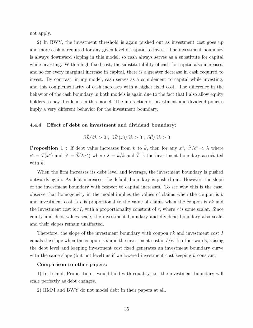
not apply.

2) In BWY, the investment threshold is again pushed out as investment cost goes up

and more cash is required for any given level of capital to invest. The investment boundary

is always downward sloping in this model, so cash always serves as a substitute for capital

while investing. With a high fixed cost, the substitutability of cash for capital also increases,

and so for every marginal increase in capital, there is a greater decrease in cash required to

invest. By contrast, in my model, cash serves as a complement to capital while investing,

and this complementarity of cash increases with a higher fixed cost. The difference in the

behavior of the cash boundary in both models is again due to the fact that I also allow equity

holders to pay dividends in this model. The interaction of investment and dividend policies

imply a very different behavior for the investment boundary.

4.4.4 Effect of debt on investment and dividend boundary:

∂I/∂k > 0 ; ∂I ′(x)/∂k > 0 ; ∂C/∂k > 0

Proposition 1 : If debt value increases from k to k, then for any x∗, c∗/c∗ < λ where

c∗ = I(x∗) and c∗ = ¯I(λx∗) where λ = k/k and ¯I is the investment boundary associated

with k.

When the firm increases its debt level and leverage, the investment boundary is pushed

outwards again. As debt increases, the default boundary is pushed out. However, the slope

of the investment boundary with respect to capital increases. To see why this is the case,

observe that homogeneity in the model implies the values of claims when the coupon is k

and investment cost is I is proportional to the value of claims when the coupon is rk and

the Investment cost is rI, with a proportionality constant of r, where r is some scalar. Since

equity and debt values scale, the investment boundary and dividend boundary also scale,

and their slopes remain unaffected.

Therefore, the slope of the investment boundary with coupon rk and investment cost I

equals the slope when the coupon is k and the investment cost is I/r. In other words, raising

the debt level and keeping investment cost fixed generates an investment boundary curve

with the same slope (but not level) as if we lowered investment cost keeping k constant.

Comparison to other papers:

1) In Leland, Proposition 1 would hold with equality, i.e. the investment boundary will

scale perfectly as debt changes.

2) HMM and BWY do not model debt in their papers at all.

35

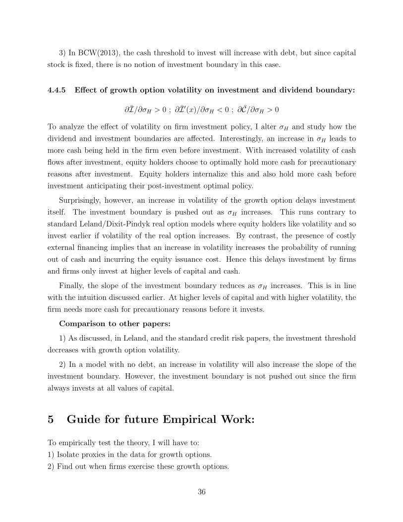
3) In BCW(2013), the cash threshold to invest will increase with debt, but since capital

stock is fixed, there is no notion of investment boundary in this case.

4.4.5 Effect of growth option volatility on investment and dividend boundary:

∂I/∂σH > 0 ; ∂I ′(x)/∂σH < 0 ; ∂C/∂σH > 0

To analyze the effect of volatility on firm investment policy, I alter σH and study how the

dividend and investment boundaries are affected. Interestingly, an increase in σH leads to

more cash being held in the firm even before investment. With increased volatility of cash

flows after investment, equity holders choose to optimally hold more cash for precautionary

reasons after investment. Equity holders internalize this and also hold more cash before

investment anticipating their post-investment optimal policy.

Surprisingly, however, an increase in volatility of the growth option delays investment

itself. The investment boundary is pushed out as σH increases. This runs contrary to

standard Leland/Dixit-Pindyk real option models where equity holders like volatility and so

invest earlier if volatility of the real option increases. By contrast, the presence of costly

external financing implies that an increase in volatility increases the probability of running

out of cash and incurring the equity issuance cost. Hence this delays investment by firms

and firms only invest at higher levels of capital and cash.

Finally, the slope of the investment boundary reduces as σH increases. This is in line

with the intuition discussed earlier. At higher levels of capital and with higher volatility, the

firm needs more cash for precautionary reasons before it invests.

Comparison to other papers:

1) As discussed, in Leland, and the standard credit risk papers, the investment threshold

decreases with growth option volatility.

2) In a model with no debt, an increase in volatility will also increase the slope of the

investment boundary. However, the investment boundary is not pushed out since the firm

always invests at all values of capital.

5 Guide for future Empirical Work:

To empirically test the theory, I will have to:

1) Isolate proxies in the data for growth options.

2) Find out when firms exercise these growth options.

36

Hypothetically, if firms behaved in the data exactly as they do in the model, CAPEX

would be zero in most periods, and would be non-zero only when exercising the growth

option. If this were the case, I can identify all quarters where the firm has non-zero CAPEX,

and also obtain the stock of the company’s capital and cash holdings in those quarters. These

would be the periods where the firm exercises the growth option.

However, in practice, CAPEX is not always zero and is fairly persistent. Therefore, to

get around this, I will obtain the median CAPEX/K ratio for each (non financial) industry,

where K is capital stock minus cash (it can also be tangible assets of the firm), and isolate

firms with high CAPEX/K in the top 10th percentile. I will consider these firms as having

exercised growth options and obtain their capital stock and cash levels to test some of the

results of the model.

6 Conclusion:

This paper builds a dynamic capital structure model of the firm with default, liquidity and

investment. Costly external financing results in a non-trivial cash policy and also leads

to liquidity risk. The firm optimally issues equity when it runs out of cash, and pays out

dividends when levels of cash are above the optimal threshold. Permanent shocks to the

firm’s capital stock result in time varying solvency for the firm and the optimal liquidity

policy is tightly connected to the firm’s solvency and results in both solvency and liquidity

risks of default.

In addition, the firm is endowed with a real option and can choose when to invest.

The presence of both long term debt resulting in an optimal strategic default policy, and

costly external financing resulting in an optimal liquidity policy distort the firm’s investment

decisions and gives rise to several novel implications. The decision to invest is a function of

both capital and cash and whether cash serves as a compliment or substitute to capital for

investment depends on the distance to default. If a firm is financially constrained and has

high credit risk prior to investment, but is less constrained after investing, then cash serves

as a substitute to capital for investment. On the other hand, if a firm is not constrained

both before and after investing, then cash serves as a complement to capital for investment.

Further, an increase in the cost of investing results in increased liquidity holdings and

reduced dividend payments even prior to investment. When the volatility of the investment

project increases, the firm also chooses to delay investing - contrary to standard growth

option literature - and holds more cash at all levels of capital (reducing dividend payments)

anticipating the risk it will face in the future after investing. If the firm increases debt levels,

37

then - holding investment cost fixed - the firm is likely to invest at higher leverage, and the

complementarity of cash for investment decreases.

In future work, I will focus on trying to empirically test some of the novel results from

the model.

38

Figure 4: Effect of volatility on cash boundary

This figure plots the optimal cash boundary for a firm for different values of cash flow volatility (σ). Theparameters used are µ = 5%, k = 10, r = 6. The red line shows the cash boundary when σ = 19%, whilethe blue line shows the boundary when σ = 23.75%. The capital stock, X is shown on the X-axis, whilecorresponding cash levels, C is shown on the Y-axis.

200 400 600 800 1000 1200 1400 16000

50

100

150

200

250

300

350

Capital

Cas

h

cash bdy (high vol)cash bdy (low vol)

39

Figure 5: Effect of cash flow growth on cash boundary

This figure plots the optimal cash boundary for a firm for different values of cash flow growth (µ). Theparameters used are σ = 19%, k = 10, r = 6%. The red line shows the cash boundary when µ = 4%,while the blue line shows the boundary when µ = 5%. The capital stock, X is shown on the X-axis, whilecorresponding cash levels, C is shown on the Y-axis.

200 400 600 800 1000 1200 1400 16000

50

100

150

200

250

300

350

Capital

Cas

h

40

Figure 6: Marginal value of cash

This figure plots the marginal value of cash for a firm for different values of the fixed cost of financing (F ).The parameters used are µ = 4%, σ = 19%, k = 10, r = 6%. The green line shows the cash boundary whenF = 2 × k/r, while the blue line shows the boundary when F = k/r. The capital stock, X is shown on theX-axis, while corresponding cash levels, C is shown on the Y-axis.

41

Figure 7: Investment, dividend boundary

This figure plots the investment and dividend boundary of the firm around the point when the firm choosesto exercise the growth option. The values of µ and µH are taken to be 4% and 5% respectively, while σ andσH are taken to be 19% and 23.75% respectively. The investment cost is I = 0.03 ∗ x

900 950 1000 1050 1100 1150 1200 1250140

160

180

200

220

240

260

280

300

Capital

Cas

h

div bdy (with inv)inv bdydiv bdy (no inv)

42

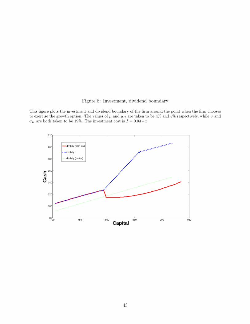
Figure 8: Investment, dividend boundary

This figure plots the investment and dividend boundary of the firm around the point when the firm choosesto exercise the growth option. The values of µ and µH are taken to be 4% and 5% respectively, while σ andσH are both taken to be 19%. The investment cost is I = 0.03 ∗ x

700 750 800 850 900 95080

100

120

140

160

180

200

220

Capital

Cas

h

div bdy (with inv)

inv bdy

div bdy (no inv)

43

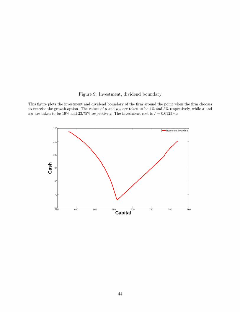
Figure 9: Investment, dividend boundary

This figure plots the investment and dividend boundary of the firm around the point when the firm choosesto exercise the growth option. The values of µ and µH are taken to be 4% and 5% respectively, while σ andσH are taken to be 19% and 23.75% respectively. The investment cost is I = 0.0125 ∗ x

620 640 660 680 700 720 740 76060

70

80

90

100

110

120

Capital

Cas

h

investment boundary

44

References

Acharya, V., Davydenko, S., Strebulaev, I., 2012. Cash holdings and credit risk. Review of

Financial Studies 25, 3572-3609.

Davydenko, S., 2013. Insolvency, illiquidity, and the risk of default. Unpublished working

paper, University of Toronto.

Bates, T., Kahle, K., Stulz, R., 2009. Why do U.S firms hold so much more cash than they

used to? Journal of Finance 64, 1985-2021.

Anderson, R., Carverhill, A., 2007. Corporate liquidity and capital structure. Review of

Financial Studies 25, 797-837.

Chen, H., 2010. Macroeconomic conditions and the puzzles of credit spreads and capital

structure. Journal of Finance 65, 2171-2212.

Leland, H.E., 1994. Corporate debt value, bond covenants, and optimal capital structure.

Journal of Finance 49, 1213-1252.

Merton, R., 1974. On the pricing of corporate debt: The risk structure of interest rates.

Journal of Finance 29, 449-470.

Riddick, L., Whited, T., 2009. The corporate propensity to save. Journal of Finance 64,

1729-1766.

Decamps, J., Mariotti, T., Rochet, J., Villeneuve, S. 2011, Free cash flow, Issuance costs,

and stock prices. Journal of Finance 66, 1501-1541.

45

A Appendix for Baseline Model

Proof of Proposition 1:

To obtain equity value on the boundary, E(x), we start by imposing the smoothpasting and

supercontact conditions on the HJB equation for equity

rE(x, c) = (µx− k)[φEx + (1− φ)Ec] +1

2σ2x2[φ2Exx+ (1− φ)2Ecc + 2φ(1− φ)Exc (12)

The smooth pasting condition states that Ec = 1 and Ecc = 0 at the boundary. Further, the

derivative of Ec along the cash boundary is given by

d

dxEc|c=C(x) = C ′(x)Ecc + Ecx

Ecc = 0 at the boundary, and Ec is constant along the boundary, implying that dEc/dx = 0

along the boundary. Therefore, the above equation implies that Ecx = 0 along the boundary.

Therefore, we can simplify the equity HJB equation to get an ODE,

rE(x, C(x)) =∂E

∂xφ(µx− k) +

1

2

∂2E

∂x2φ2σ2x2 + (1− φ)(µx− k)

The solution is given by

E(x, C(x)) = (1− φ)(µx− k)

r − µφ+ cEx

r2F (r2; x) + cE1xr1F (r1; x) (13)

where r1 and r2 are the positive and negative roots of the quadratic

1

2φ2σ2x(x− 1) + µx− r = 0

and F (r; x) denotes the Kummer function,

F (r; x) = 1F1(−r;−2r + 2−µ

(1/2)φσ2;−

k

x(1/2)φσ2)

where

1F1(a, b, z) = Σ∞j=0

a(j)

b(j)j!zj ; a(j) = a× (a+ 1)× (a + 2)× ...× (a + j − 1)

As x → ∞, the expected future earnings of the firm diverges, and so the expected

probability of default vanishes to zero. At the optimal cash boundary, the value of equity

46

is then equal to the expected future cash flow net of liabilities, i.e. limx to∞ E(x, C(x)) =µx

r−µ− k

r. Substituting this condition in the above expression for equity, we see that cE1 = 0.

To get cE , we use the default condition. At the point of solvency default, the optimal cash

boundary goes to zero since debt holders claim any residual cash in the firm. Thus the firm

is always at the cash boundary at default, and so we set the above expression to zero at

default to obtain cE.

We get that cE = −[ µxd

r−µ− k

r]x−r2

d F (r2; xd)−1. Substituting this value in the above expression

for equity, we obtain the result.

Proof of Proposition 2: The functional forms of q1(x, c) and q2(x, c) are given by

q1(x, c) =

(

xxl

)r1F (r1,x)F (r1,xl)

−(

xxl

)r2F (r2,x)F (r2,xl)

(

xu

xl

)r1F (r1,xu)F (r1,xl)

−(

xu

xl

)r2F (r2,xu)F (r2,xl)

q2(x, c) =

(

xxu

)r1F (r1,x)F (r1,xu)

−(

xxu

)r2F (r2,x)F (r2,xu)

(

xl

xu

)r1F (r1,xl)F (r1,xu)

−(

xl

xu

)r2F (r2,xl)F (r2,xu)

To prove this result, we will first derive the values of q1(x, c) and q2(x, c), which are (respt.)

contracts that pay $1 when the total earnings of the firm is at either xu or xl. To derive the

values of these securities, we first use the fact that q1 is a traded asset and so satisfies the

following equation

rq1(x, c) = (∂q1∂x

+∂q1∂c

)(µx− k) +1

2σ2x2(

∂2q1∂x2

+∂2q1∂c2

+ 2∂2q1∂x∂c

)

This is a parabolic PDE that can be solved by a change of variables.

Let ξ(x, c) = c− x ; η(x, c) = x. Then, we have the following relations (where subscripts

denote partial derivatives):

q1x = q1η − q1ξ ; q1xx = q1ηη + q1ξξ − 2q1ηξ ; q1xc = q1ηξ − q1ξξ

q1c = q1ξ ; q1cc = q1ξξ

Making these transformations, the above PDE reduces to

rq1(η, ξ) = (∂q1∂η

(µη − k) +1

2σ2η2(

∂2q1∂η2

This has the solution q1(x, c) = c1(ξ)xr1F (r1; x) + c2(ξ)x

r2F (r2; x). Note that ξ = (x −

47

c) = xl. I will revert to using xl in the remainder of the proof to be consistent with the

paper. Using the conditions that q1(xu, c(xu) = 1 and q1(xl, c(xu) = 0, we have that c1 and

c2 satisfy the following conditions:

c1xr1u F (r1; xu) + c2x

r2u F (r2; xu) = 1 ; c1x

r1l F (r1; xl) + c2x

r2l F (r2; xl) = 0

Solving for c1 and c2 in terms of xu and xl from the above two equations gives us the result.

Proof of Proposition 3:

Since vt is a traded claim, it satisfies the equation

rv(x, C(x)) =∂v

∂x(µx− k) +

1

2

∂2v

∂x2σ2x2 +

∂v

∂CC ′(x)dx+

1

2

∂2v

∂C2σ2x2

Using the smooth pasting conditions ∂v∂C

= 0, we are left with the PDE,

rv(x, C(x)) =∂v

∂x(µx− k) +

1

2

∂2v

∂x2σ2x2 +

1

2

∂2v

∂C2σ2x2

This is a parabolic PDE that can be solved as before by a change of variables.

Indeed, define

ξ = c− x ; η = x

Making these substitutions, the above PDE reduces to an ODE,

rv =1

2σ2η2vηη + (µη − k)vη

This has the solution

v(ξ, η) = A(ξ)ηr1F (r1; η)

where A(.) is an arbitrary function.

Note that by smooth pasting, vξ = vc = 0. This in turn implies that A′(ξ) = 0, and so A(.)

is a constant.

Substituting the boundary condition, v(xd) = 1 gives the result.

Proof of Proposition 4:

The proof follows the same steps as when we obtain boundary values for equity. Since debt

is a traded asset, it follows the partial differential equation,

rB(x, C(x)) = k +∂B

∂x(µx− k) +

1

2

∂2B

∂x2σ2x2 +

∂B

∂CC ′(x)dx+

1

2

∂2B

∂C2σ2x2

48

We can again change variables by defining ξ = c− x ; η = x

Making this change in variables and solving the resultant ODE gives us

B(x, c) = A(ξ)xr2F (r2; x) + kr

On the boundary, by smooth pasting, ∂B∂c

= ∂B∂ξ

= 0. Therefore, A′(ξ) = 0 on the boundary,

and so A(ξ) is constant (=A, say).

At the point of solvency default, B(xd, 0) = Axr2d F (r2; xd) + kr = α µxd

r−µ.

Therefore,

A =

(

α µxd

r−µ− k

r

)

xr2d F (r2, xd)

Substituting this value of A in the expression above, we get that

B(x, C(x)) =k

r+

(

αµ

(r − µ)xd −

k

r

)

xr2F (r2, x)

xr2d F (r2, xd)

This proves the result.

Proof of Proposition 7: Since the default boundary is chosen optimally, the smooth

pasting condition must hold, i.e. ∂E(x)/∂x = 0 at default. Using the value of E defined in

5, taking the derivative w.r.t x and setting it equal to 0, we obtain the result.

Proof of Proposition 8: To prove equation 9, note that ∂E(x, c)/∂c = 1 at the cash

boundary.

Also, the total derivative dE(x, c)/dx is given by

d

dxE(x, c) =

∂

∂cE(x, c)

(1− φ)

φ+

∂

∂xE(x, c)

In general, note that E ′(x) = ∂E(x, c)/∂x + ∂E(x, c)/∂cC ′(x)

Since ∂E(x, c)/∂c = 1 at the cash boundary, we have that ∂E(x, c)/∂x =

Therefore, as x → xu,

d

dxE(x, c) =

(1− φ)

φ+ E ′(x)− C ′(x)

proving the proposition in the text.

The full form of the cash boundary is given by:

49

x′u(xl) =

[

1xl(r1(

xu

xl)r1−1 F (r1,xu)

F (r1,xl)− r2(

xu

xl)r2−1 F (r2,xu)

F (r2,xl)) + (xu

xl)r1 G(r1,xu)

F (r1,xl)+ (xu

xl)r2 G(r2,xu)

F (r2,xl)(

xu

xl

)r1F (r1,xu)F (r1,xl)

−(

xu

xl

)r2F (r2,xu)F (r2,xl)

E(xu)

−

(

(1− φ)µ

r − µAφ+ cE(r2x

r2−1u F (r2; xu) + xr2

u G(r2; xu))

)

+ ...

+

1xu(r2 − r1) +

G(r2,xu)F (r2,xu)

− G(r1,xu)F (r1,xu)

(

xl

xu

)r2F (r2,xl)F (r2,xu)

−(

xl

xu

)r1F (r1,xl)F (r1,xu)

[

max(0, E(xℓ)− Fc − C(xℓ))]

]−1

C(xu) = xu − xℓ(1− φ)/φ

cE = −[(1− φ)(µxd − k)

r − µφ](1

xd

)r21

F (r2; xd)

xu(D) = 0

To prove the result, we follow several steps. First recall that the cash boundary is obtained

by plugging in the Smooth Pasting condition:

limC→C(x)

∂E

∂C= 1

where subscripts denote partial derivatives. To determine the cash boundary, we have to

determine the form of the function xu(.), where xu(.) maps values of xl to values of xu. In

particular, xu is the X-coordinate of the point where the 45◦ line drawn from xl intersects

the cash boundary. Note that if xu(.) is determined, the cash boundary is automatically

obtained as well. From now on, I will slightly abuse notation and reference xu as xu(xl).

This serves two purposes: One is to lower the burden of notation by eliminating the need to

keep referencing xu(.). The other is to emphasize that xu is a function of xl and is completely

determined by xl. In particular, there exists a unique xu for any given value of xl.

With this notation, we can write

q1,c(x = xu) =x′u(xl)

1xl(r1(

xu

xl)r1−1 F (r1,xu)

F (r1,xl)− r2(

xu

xl)r2−1 F (r2,xu)

F (r2,xl)) + (xu

xl)r1 G(r1,xu)

F (r1,xl)+ (xu

xl)r2 G(r2,xu)

F (r2,xl)(

xu

xl

)r1F (r1,xu)F (r1,xl)

−(

xu

xl

)r2F (r2,xu)F (r2,xl)

q2,c(x = xu) = x′u(xl)

1xu(r2 − r1) +

G(r2,xu)F (r2,xu)

− G(r1,xu)F (r1,xu)

(

xl

xu

)r2F (r2,xl)F (r2,xu)

−(

xl

xu

)r1F (r1,xl)F (r1,xu)

In the above, G(r, z) = F ′(r, z) where the derivative is with respect to z. Also, since, by

50

definition, xu lies on the cash boundary, we have that

E(xu) = E(xu, C(xu)) =µxu

r − µ−

k

r − µ+ cEx

r2u F (r2; xu)

Therefore,

Ec(xu) = Ec(xu, C(xu)) = −x′u(xl)[

µ

r − µ+ cE

d

dxu

(xr2u F (r2; xu))]

We can now obtain the partial derivative Ec(.) at x = xu. Substituting the fact that q1 = 1

and q2 = 0 at x = xu, we get

Ec(x, c) =

q1,c(xu)E(xu) + Ec(xu) + q2,c(xu)(

E(xl)− F − C(xl))

, if E(xl) > F + C(xl)

q1,c(xu)E(xu) + Ec(xu), otherwise.

Let x be such that E(x) − F − C(x) < 0 for x < x. Also, let xu = xu(x). x is obtained

numerically and solves the non-linear equation

[µx

r − µ−

k

r − µ]− [

µxd

r − µ−

k

r − µ](x

xd

)r2F (r2; x)

F (r2; xd)= F + C(x)

Substituting the relevant expressions, we obtain the result.

Proof of Proposition 9: Before proving the result, we first prove the following lemma:

Lemma 1: In the hoarding region, the marginal value of cash is greater than 1.

This lemma formally shows that the optimal dividend policy for the firm is a threshold

policy - i.e. the firm pays out dividends when cash levels reach a particular threshold which

is the cash boundary. To prove this, I will show that the total derivative dEc/dx < 0, where

Ec = ∂E/∂c. This result implies the Lemma since Ec = 1 at the boundary.

Proof: The firm has capital level X and cash level C that evolves according to the

following process

dXt = Aφ(µXtdt+ σXtdWt − kdt)

dCt = (1− φ)(µXtdt+ σXtdWt − kdt) =1− φ

AφdXt

When the firm is hoarding cash, equity follows the usual evolution equation

rE(x, C) =∂E

∂x(dx) +

∂E

∂C(dc) +

1

2

∂2E

∂x2(dx)2 +

1

2

∂2E

∂c2(dc)2 +

∂2E

∂x∂c(dx)(dc)

51

Note that dc = (1− φ)/Aφdx.

For any function f ,∂f(.)

∂x+

(1− φ)

Aφ

∂f(.)

∂c=

df(.)

dx

∂2f(.)

∂x2+

(1− φ)2

A2φ2

∂2f(.)

∂c2+ 2

(1− φ)

Aφ

∂2f(.)

∂x∂c=

d2f(.)

dx2

We can therefore rewrite the evolution equation for equity as

rE(x, C) =dE

dx(dx) +

1

2

d2E

dx2(dx)2

Differentiating the above equation with respect to c, and letting subscripts denote partial

derivatives, we get that

rEc =dEc

dx(dx) +

1

2

d2Ec

dx2(dx)2 (14)

Now, at the boundary, Ec = 1. The total derivative along the cash boundary of Ec is given

by dEc/dx = Ecx + C−1(x)Ecc Since Ec = 1 at every point on the boundary, dEc/dx = 0.

Together with the supercontact condition, this implies that Ecc = Ecx = 0 at the cash

boundary.

Equation 1 evaluated at the boundary implies therefore that d2Ec/dx2 is positive at the

boundary, and so dEc/dx < 0 in a neighborhood around the boundary.

Let x∗ = supx∈ldEc(x)/dx = 0, where l denotes the tan−1((1 − φ)/Aφ) line. Since

dEc/dx < 0 for x > x∗ and since Ec = 1 on the boundary, we have that Ec(x∗) > 1.

But, by the definition of x∗, d2Ec/dx2 < 0.

Therefore, at x∗, dEc/dx = 0, d2Ec/dx2 < 0 and Ec > 1. But this is not possible from

Equation 1, leading to a contradiction in our assumption of the existence of x∗.

Therefore, dEc(x, c)/dx < 0 for all x ∈ l.

This proves Lemma 1.

Corollary 1: ∂2E/∂C2 < 0

Proof: Recall that the boundary ∂E/∂C = 1. Since the cash boundary is increasing,

and using the lemma above, this means that ∂2E/∂x∂C > 0 at the boundary. But, since

d(Ec)/dx < 0 at the boundary, this implies that ∂2E/∂C2 < 0 at the boundary.

We have that

rEcc =dEcc

dx(dx) +

1

2

d2Ecc

dx2(dx)2

Since Ecc < 0 at the boundary, dEcc/dx > 0 at the boundary. Now, assume that there exists

a point, say P where dEcc/dx = 0, and that dEcc/dx > 0 on the line l after P . This means

52

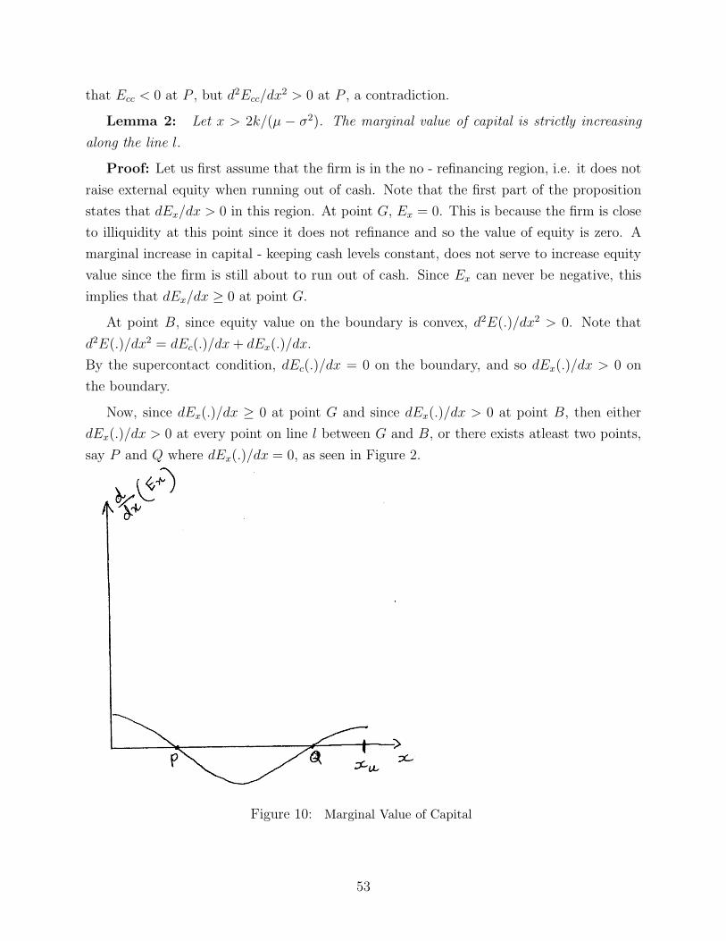
that Ecc < 0 at P , but d2Ecc/dx2 > 0 at P , a contradiction.

Lemma 2: Let x > 2k/(µ − σ2). The marginal value of capital is strictly increasing

along the line l.

Proof: Let us first assume that the firm is in the no - refinancing region, i.e. it does not

raise external equity when running out of cash. Note that the first part of the proposition

states that dEx/dx > 0 in this region. At point G, Ex = 0. This is because the firm is close

to illiquidity at this point since it does not refinance and so the value of equity is zero. A

marginal increase in capital - keeping cash levels constant, does not serve to increase equity

value since the firm is still about to run out of cash. Since Ex can never be negative, this

implies that dEx/dx ≥ 0 at point G.

At point B, since equity value on the boundary is convex, d2E(.)/dx2 > 0. Note that

d2E(.)/dx2 = dEc(.)/dx+ dEx(.)/dx.

By the supercontact condition, dEc(.)/dx = 0 on the boundary, and so dEx(.)/dx > 0 on

the boundary.

Now, since dEx(.)/dx ≥ 0 at point G and since dEx(.)/dx > 0 at point B, then either

dEx(.)/dx > 0 at every point on line l between G and B, or there exists atleast two points,

say P and Q where dEx(.)/dx = 0, as seen in Figure 2.

< Insert Fig2 here >

Figure 10: Marginal Value of Capital

53

Recall that equity, E, satisfies the ODE,

rE =dE

dx(dx) +

1

2

d2E

dx2(dx)2 (15)

where dx = Aφ(µXtdt+ σXtdWt − kdt) = µXtdt− kdt+ σXtdWt

Taking the partial derivative of the above with respect to x, we get

rEx =dEx

dx(µx− k) +

1

2

d2Ex

dx2σ2x2 + µ

dE

dx+ σ2x

d2E

dx2

We can rewrite this as

rEx − µdE

dx− σ2x

d2E

dx2=

dEx

dx(µx− k) +

1

2

d2Ex

dx2σ2x2 (16)

We can divide equation 2 by x to get that

rE

x= (µ−

k

x)dE

dx+

1

2σ2x

d2E

dx2

This implies that

µdE

dx+

1

2σ2x

d2E

dx2=

rE

x+

k

x

dE

dx

Equation 3 can then be re-written as

rEx −rE

x−

k

x

dE

dx−

1

2σ2x

d2E

dx2=

dEx

dx(µx− k) +

1

2

d2Ex

dx2σ2x2

Or, after multiplying by x,

rxEx − rE − k(Ex + Ec)−1

2σ2x2d

2E

dx2= x(µx− k)

dEx

dx+

1

2σ2x2d

2Ex

dx2(17)

Equation 4 holds for all x. We will evaluate equation 4 and points P and Q. Clearly, sincedEx

dx= 0 at P and Q, and since d2Ex

dx2 < 0 at P and > 0 at Q, we have that the RHS of 4 is

higher at Q than at P .

We will derive a contradiction by showing that the LHS of equation 4 is higher at P than

at Q. More formally, if f(x, c) denotes the LHS of Equation 4, then we will show that

∫ x=Q

x=P

df(x, c)

dxdx < 0

54

where (with η = (1− φ)/Aφ)

f(x, c) = rxEx − rE − k(Ex + ηEc)−1

2σ2x2d

2E

dx2

Taking the derivative of f(.), we see that

df(x, c)

dx= rEx + rx

dEx

dx− r

dE

dx− k

d(Ex + ηEc)

dx−

1

2σ2x2d

2(Ex + ηEc)

dx2− σ2x

d(Ex + ηEc)

dx

= −rηEc +dEx

dx[rx− k − σ2x]− η

dEc

dx[k + σ2x]−

1

2σ2x2d

2(Ex + ηEc)

dx2

= −2rηEc +dEx

dx[rx− k − σ2x]− η

dEc

dx[k + σ2x+ k − µx]−

1

2σ2x2d

2Ex

dx2

where we use the fact (from Equation 1) that

−1

2

d2Ec

dx2σ2x2 = −rEc +

dEc

dx(µx− k)

Now, if 2k− µx+ σ2x < 0 and rx− k − σ2x > 0, and using our result that dEc/dx < 0 and

our assumption that dEx/dx < 0 in the region between P and Q, we see that

−2rEc +dEx

dx[rx− k − σ2x]− η

dEc

dx[k + σ2x+ k − µx] < 0

The two conditions are equivalent to x > 2k/(µ − σ2) and x > k/(r − σ2) Recall that we

need to show that∫ x=Q

x=P

df(x, c)

dx< 0

We will therefore be done if we can show that

∫ x=Q

x=P

−1

2σ2x2d

2Ex

dx2dx < 0 =⇒

∫ x=Q

x=P

x2d2Ex

dx2dx > 0

Let g = dEx

dx. Note that g = 0 at points P and Q. Now,

∫ x=Q

x=P

x2 dg

dxdx =

[

x2g]Q

P−

∫ x=Q

x=P

2xg dx = −2

[

(xEx)QP −

∫ x=Q

x=P

Exdx

]

Recall that, by definition,

Ex|x=P > Ex|x=Q =⇒ (xEx)QP = qEx|x=Q − pEx|x=P < (q − p)Ex|x=Q

55

Also,∫ x=Q

x=P

Exdx > (q − p)Ex|x=Q

Together, these conditions imply that

(xEx)QP −

∫ x=Q

x=P

Exdx < (q − p)Ex|x=Q − (q − p)Ex|x=Q = 0

In turn, this leads to

∫ x=Q

x=P

x2 dg

dxdx = −2

[

(xEx)QP −

∫ x=Q

x=P

Exdx

]

> 0

Therefore,∫ x=Q

x=P

df(x, c)

dx< 0

and so the LHS of Equation 4 is decreasing in x between P and Q. However, the RHS of

Equation 4 is higher at Q than at P , leading to a contradiction to the existence of P and Q.

Therefore, we can conclude that dEx/dx = 0 at atmost one point on the line l.

If the firm does not refinance, Ex|x=G = 0, and so d(Ex)/dx|x=G ≥ 0. Therefore, since

dEx/dx > 0 in a neighborhood around point B, we must have that d(Ex)/dx > 0 along line

l.

Now, if the firm is in the refinancing region, and raises equity at point G, then E(x)|x=G ≈

E(x)|x=Q − F − C(xu)− (xu − x), where xu is the abscissa of the point Q at which the firm

jumps to. Since the marginal value of cash is always greater than 1, the firm always finds it

optimal to jump to a point on the boundary.

Note that

E(x)|x=Q =(µxu − k)

r − µ+ cEx

r2u F (r2, xu)

Therefore,

∂E

∂x|x=G = x′

u(x)[µ

r − µ+ cEr2x

r2−1u F (r2, xu) + cEx

r2u G(r2, xu)− C ′(xu)− 1] + 1

d

dx

∂E

∂x|x=G =

d

dxx′u(x)[

µ

r − µ+ cEr2x

r2−1u F (r2, xu) + cEx

r2u G(r2, xu)− C ′(xu)− 1]

56

But, note that along line l, xu is constant, and so

d

dxxu =

d

dxx′u(x) =

d

dxF (r2, xu) =

d

dxG(r2, xu) =

d

dxC ′(xu) = 0

Therefore, when the firm is in the refinancing region, d(Ex)/dx|x=G = 0.

Further, using the arguments developed in this proof, there cannot exist two points P

and Q where dEx/dx = 0. This implies that dEx/dx is always positive along line l. This

proves the lemma.

Now we can turn to proving the Proposition.

Note that we can write

E ′(x, c, σ) =∂E

∂CC ′(σ) +

∂E

∂σ

It is straightforward to show that E ′(x, c, σ) > 0. Therefore, we can show that C ′(σ) > 0 if

we can show that ∂E∂σ

< 0.

Now, in the hoarding region, we can use the usual PDE to characterize equity value,

rE(x, C) =∂E

∂x(µx− k) +

1

2

∂2E

∂x2σ2x2 +

∂E

∂CC ′(x)(µx− k) +

1

2

∂2E

∂C2σ2x2 +

∂2E

∂C∂Xσ2x2

Let us denote the infinitesimal generator by A, so we write

rE(x, C) = AE(x, C)

By the change of variables ξ = C − x and η = C, we can rewrite the above PDE as

rE(ξ, η) =∂E

∂η(µη − µξ − k) +

1

2

∂2E

∂η2σ2(η − ξ)2

Let Eσ denote ∂E∂σ

. Differentiating the above equation by σ, we get that

rEσ(ξ, η) =∂Eσ

∂η(µη − µξ − k) +

1

2

∂2Eσ

∂η2σ2(η − ξ)2 +

∂2E

∂η2σ(η − ξ)2

Re-changing back to the original coordinates, we get that

rEσ = AEσ(x, C) + σx2∂2E

∂C2

We have shown already that ∂2E∂C2 < 0 from Lemma 1, and so we have that −rEσ +AEσ > 0.

We will be done if we can show that limT→∞ e−rTEσ(x, C) = 0, which is true.

57

We now prove the second part of the proposition: that cash boundary is decreasing in cash

flow growth. The proof will be along the same lines as the previous result.

Note that we can write

E ′(x, c, µ) =∂E

∂CC ′(µ) +

∂E

∂µ

We can show that C ′(µ) < 0 if we can show that E ′(x, c, µ)− ∂E∂µ

< 0.

Now, in the hoarding region, we can use the usual PDE to characterize equity value,

rE(x, C) =∂E

∂x(µx− k) +

1

2

∂2E

∂x2σ2x2 +

∂E

∂C(µx− k) +

1

2

∂2E

∂C2σ2x2 +

∂2E

∂C∂Xσ2x2

Let us denote the infinitesimal generator by A, so we write

rE(x, C) = AE(x, C)

Let Eµ denote ∂E∂µ

. Differentiating the above equation by µ, we get that

rEµ(x, C) = AEµ(x, C) + x(∂E

∂x+

∂E

∂c)

Clearly, (∂E∂x

+ ∂E∂c) > 0 in the hoarding region, and so we have that −rEµ + AEµ < 0.

We will be done if we can show that limT→∞ e−rTEµ(x, C) = 0, which is true.

B Appendix for Real Option Model:

Expressions for functions in Proposition 10:

Before proving the proposition, I will explicitly list out the expression for functions not

listed in the main text. The expressions for q1(x, c) and q2(x, c) are the same as that listed

earlier. q1 and q2 are given by

q1(x, c) =

(

xxl

)r1F (r1,x)F (r1,xl)

−(

xxl

)r2F (r2,x)F (r2,xl)

(

x∗

xl

)r1F (r1,x∗)F (r1,xl)

−(

x∗

xl

)r2F (r2,x∗)F (r2,xl)

q2(x, c) =

(

xx∗

)r1 F (r1,x)F (r1,x∗)

−(

xx∗

)r2 F (r2,x)F (r2,x∗)

(

xl

x∗

)r1 F (r1,xl)F (r1,x∗)

−(

xl

x∗

)r2 F (r2,xl)F (r2,x∗)

q1λ is the values of a claim that pays a dollar when the capital in the firm hits the

threshold xu and the firm has not invested, i.e. has not been hit by the real investment

58

shock. By the Ito Formula, q1λ is given by the following equation,

rq1λ(x, c) = (µx− k)dq1λdx

+1

2σ2x2d

2q1λdx2

+ λ(0− q1λ) ; q1λ(xu) = 1 ; q1λ(x∗) = 0

Similarly, q2λ is the value of a claim that pays a dollar when the capital in the firm hits the

threshold x∗ and the firm has not invested. It’s value is given by

rq2λ(x, c) = (µx− k)dq2λdx

+1

2σ2x2d

2q2λdx2

+ λ(0− q2λ) ; q2λ(xu) = 0 ; q2λ(x∗) = 1

Let r1λ and r2λ be the positive and negative roots of the equation

1

2φ2σ2x(x− 1) + µφx− (r + λ) = 0

Then, q1λ and q2λ are given by

q1λ(x, c) =

(

xx∗

)r1λ F (r1λ,x)F (r1λ,x∗)

−(

xx∗

)r2λ F (r2λ,x)F (r2λ,x∗)

(

xu

x∗

)r1λ F (r1λ,xu)F (r1λ,x∗)

−(

xu

x∗

)r2λ F (r2λ,xu)F (r2λ,x∗)

q2λ(x, c) =

(

xxu

)r1λ F (r1λ,x)F (r1λ,xu)

−(

xxu

)r2λ F (r2λ,x)F (r2λ,xu)

(

x∗

xu

)r1λ F (r1λ,x∗)F (r1λ,xu)

−(

x∗

xu

)r2λ F (r2λ,x∗)F (r2λ,xu)

Note that q1, q2, q1 and q2, q1λ and q2λ satisfy q1(xu, C(xu)) = q2(xℓ, 0) = q1(x∗, c∗) =

q2(xℓ, 0) = q1λ(xu, C(xu)) = q2λ(x∗, c∗) = 1.

Also, q1(xℓ, 0) = q2(xu, C(xu)) = q1(xℓ, 0) = q2(x∗, c∗) = q1λ(x

∗, c∗) = q2λ(xu, C(xu)) = 0

Finally, Ep(x, c) is given by

Ep(x, c) = a1pxr1HF(r1H , r1λ, x) + a2px

r2HF(r2H , r2λ, x)

where r1λ and r2λ are defined as before. r1H and r2H are the roots of x2 +2µH/σ2x− r = 0.

F(rH, rλ, x) =∞∑

i=0

(cH)i1

σi(σi + c− 1)× zi2F2(1, σi + a; σi + 1, σi + c;−z)

where σi = −rH − rλ + i, a = rλ, c = −2µ/σ2+2+2rλ, (cH)i = [(aH)i× (−1)i]/[(bH)ii!] and

where

2F2(a, b; c, d; z) =∞∑

i=0

(a1)i(a2)izi

(b1)i(b2)ii!

59

is the generalized Hypergeometric Function.

Finally, a1p = −a1H/(0.5φ2σ2) and a2p = −a2H/(0.5φ

2σ2), where

a1H =EHℓ(xuH)

r2HF (r2H , xuH)−EHu(xℓH)r2HF (r2H , xℓH)

(xℓH)r1H (xuH)r2HF (r1H , xℓH)F (r2H , xu)− (xℓH)r2H (xuH)r1HF (r2H , xℓH)F (r1H , xu)

a2H =EHu(xℓH)

r1HF (r1H , xℓH)−EHℓ(xuH)r1HF (r1H , xuH)

(xℓH)r1H (xuH)r2HF (r1H , xℓH)F (r2H , xu)− (xℓH)r2H (xuH)r1HF (r2H , xℓH)F (r1H , xu)

Proof of Proposition 10: We can now prove the result.

From earlier work, we know that EH(x) can be written as

EH(x, c) = a1Hxr1HF (r1H , x) + a2Hx

r2HF (r2H , x)

where

F (r, x) = 1F1(−r;−2r + 2− 2µH

φσ2;−2

k

xφσ2)

where

1F1(a, b; z) =

∞∑

i=0

(a)izi

(b)ii!

denotes the Kummer Hypergeometric Function and where (a)i = a(a+ 1)× ...× (a+ i− 1)

is the pochhammer symbol, and where EHℓ and EHu are equity values at xuH and at xℓH

respectively.

This explicit expression for EH will now help us solve for E(x, c) - the equity value before

exercising the option.

Consider the equation

rE = (µx−k) (φEx + (1− φ)Ec)+1

2σ2x2

(

φ2Exx + 2φ(1− φ)Exc + (1− φ)2Ecc

)

+λ (EH(x, c− I)− E(x, c))

Then by changing variables η = x and ξ = c− x, the PDE reduces to an ODE

rE = (µx− k)dE

dx+

1

2σ2x2d

2E

dx2+ λ (EH(x, c− I)− E(x, c)) ,

or

(r + λ)E = (µx− k)dE

dx+

1

2σ2x2d

2E

dx2+ λEH(x, c− I)

60

Writing out EH(x, c) = a1Hxr1HF (r1H , x) + a2Hx

r2HF (r2H , x), it remains to solve

(r + λ)E = (µx− k)dE

dx+

1

2σ2x2d

2E

dx2+ λa1Hx

r1HF (r1H , x) + λa2Hxr2HF (r2H , x)

This can be rewritten as

(r + λ)E = L(E) + λa1Hxr1HF (r1H , x) + λa2Hx

r2HF (r2H , x)

Therefore, we can write E(x) = E(x) + λE1p(x) + λE2p(x) where E(x) is the solution to

the homogeneous equation (r + λ)E = L(E) ; E1p is a particular solution to the equation

(r + λ)E = L(E) + λa1Hxr1HF (r1H , x), and E2p is a particular solution to the equation

(r + λ)E = L(E) + λa2Hxr2HF (r2H , x).

From earlier work, we know that E(x) = a1λxr1λF (r1λ, x) + a2λx

r2λF (r2λ, x) where r1λ

and r2λ are roots of x2 + 2µH/σ2x− (r + λ) = 0 and a1λ and a2λ are given by

a1λ =(E∗ − λE∗

p)(xu)r2λF (r2λ, xu)− (Eu − λEp(xu))(x

∗)r2λF (r2λ, x∗)

(x∗)r1λ(xu)r2λF (r1λ, x∗)F (r2λ, xu)− (xu)r1λ(x∗)r2λF (r1λ, xu)F (r2λ, x∗)

a2λ =(Eu − λEp(xu))(x

∗)r1λF (r1λ, x∗)− (E∗ − λE∗

p)(xu)r1λF (r1λ, xu)

(x∗)r1λ(xu)r2λF (r1λ, x∗)F (r2λ, xu)− (xu)r1λ(x∗)r2λF (r1λ, xu)F (r2λ, x∗)

and where Ep(x) = E1p(x) + E2p(x).

I will now detail how to obtain E1p. E2p is obtained in an identical manner.

Recall that E1p solves (r + λ)E = L(E) + λa1Hxr1HF (r1H , x). Now, define z = k/x

and change variables. Also, let us divide throughout by 1/2σ2. To that end, define µ =

µ/((1/2)σ2), r = r/((1/2)σ2) and λ = λ/((1/2)σ2). Let s(z) be a function that satisfies

the above inhomogeneous ODE. Then dz/dx = −k/x2 = −z2/k. Therefore, ds/dx =

−s′(z)z2/k. Also d2s/dx2 = z2/k[s′′(z)z2/k + 2zs′(z)/k]. Plugging these expressions into

the terms in the ODE, we get that

(µx− k)ds/dx = −µzs′(z) + z2s′(z) ; x2d2s/dx2 = z2s′′(z) + 2zs′(z)

Substituting these expressions in the ODE we get

(r + λ)s = s′(z)[

−µz + z2 + 2z]

+ z2s′′(z) + λa1Hxr1HF (r1H , x)

Let s(z) = zγG(.). Then s′(z) = γzγ−1G(.) + zγG′(.). Also, s′′(z) = γ(γ − 1)zγ−2G(.) +2γzγ−1G′(.) + zγG′′(.).

61

Plugging these into the ODE, we get

(r + λ)zγG =(

γzγG+ zγ+1G′)

[−µ+ z + 2] +(

γ(γ − 1)zγG+ 2γzγ+1G′ + zγ+2G′′)

+ λa1Hxr1HF (r1H , x)

= zγG [−µγ + 2γ + γ(γ − 1)] + γzγ+1G+ zγ+1G′(−µ+ z + 2+ 2γ) + zγ+2G′′ + λa1Hxr1HF (r1H , x)

Set (r + λ) = −µγ + 2γ + γ(γ − 1). Then, we get that

γzγ+1G+ zγ+1G′(−µ+ z + 2 + 2γ) + zγ+2G′′ + λa1Hxr1HF (r1H , x) = 0

After simplifying,

γG+G′(−µ+ 2 + 2γ + z) + zG′′ = −λak1Hz−r1H−γ−1F (r1H , x) (18)

where ak1H = a1H/kr1H .

Lemma: If y(x, σ) is a particular solution to the differential equation x dy

dx2 +(c+x) dydx

+

ay = xσ−1, then

y(x, σ) = xσ

∞∑

i=0

aixi ; a0 =

1

σ(σ + c− 1); an+1 =

−an(σ + a+ n)

(σ + c + n)(σ + n+ 1)

Proof: This is immediate when writing y out as a series, evaluating derivatives and matching

coefficients. �

Now, recall that F (r1H , x) = 1F1(aH ; bH ;−z) =∑∞

i=0(cH)izi.

Therefore, λak1Hz−r1H−γ−1F (r1H , x) = λak1H [

∑∞

i=0(cH)izσi−1] where σi = −r1H−γ+i Using

the Lemma above, if Gp(z) is the particular solution to equation 1, then we can write

Gp(z) = −λak1H

∞∑

i=0

(cH)iy(z, σi)

Note that

y(z, σi) =1

σi(σi + c− 1)zσi

2F2(1, σi + a; σi + 1, σi + c;−z)

Finally, note that

E1p(x) = zγGp(z) = −λak1Hzγ

∞∑

i=0

(cH)iy(z, σi)

Changing variables back from z to x and canceling out some exponents gives the result. E2p

is obtained similarly. This completes the proof.

62

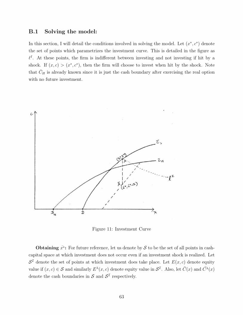
B.1 Solving the model:

In this section, I will detail the conditions involved in solving the model. Let (x∗, c∗) denote

the set of points which parametrizes the investment curve. This is detailed in the figure as

ℓI . At these points, the firm is indifferent between investing and not investing if hit by a

shock. If (x, c) > (x∗, c∗), then the firm will choose to invest when hit by the shock. Note

that CH is already known since it is just the cash boundary after exercising the real option

with no future investment.

Figure 11: Investment Curve

Obtaining x∗: For future reference, let us denote by S to be the set of all points in cash-

capital space at which investment does not occur even if an investment shock is realized. Let

SI denote the set of points at which investment does take place. Let E(x, c) denote equity

value if (x, c) ∈ S and similarly Eλ(x, c) denote equity value in SI . Also, let C(x) and Cλ(x)

denote the cash boundaries in S and SI respectively.

63

Then, we can show that in region S, equity value on the boundary, E(x) is given by

E(x) =µx− k

r − µ+ cE1x

r1F (r1, x) + cE2xr2F (r2, x)

Similarly, in region SI ,

Eλ(x) =µx− k

r + λ− µ+ cλEx

r2λF (r2λ, x) + λE1p(x, Cλ(x)) + λE2p(x, Cλ(x))

Let us also assume that the firm defaults at D if it has not exercised the real option.

Clearly, (D, 0) ∈ S. Then, the unknowns when solving for equity value on the boundary in

both regions are D, cE1, cE2, cλE , x∗, C(x∗), Cλ(x∗).

Solving the system: I impose a number of optimality conditions to solve for the

variables. Firstly, we have value matching and smooth pasting conditions at default. Further,

value matching of E must occur at x∗. Also, since by definition the firm is indifferent between

investing and not investing at x∗, we must have that E(x∗) = EH(x∗, C(x∗) − I). Finally,

there should be a smooth pasting condition at x∗ that I will go over separately. To summarize,

the conditions can be written as

• E(D) = 0 (Value-Matching at default)

• E ′(D) = 0 (Smooth-Pasting at default)

• E(x∗) = Eλ(x∗) (Value Matching at x∗)

• E(x∗) = EH(x∗, C(x∗)− I) (By definition of x∗)

• Smooth-Pasting at x∗

• Ecc(x∗) = 0 (Super-contact condition at C(x∗).

Smooth-Pasting Conditions: There will in general be two separate smooth pasting

conditions depending on whether x∗ is on the boundary (i.e. x∗ = x∗) or not. If x∗ is not

on the boundary, then the value matching and smooth pasting conditions at x∗ will take the

form E(x∗, c∗) = Eλ(x∗, c∗) and dE(x∗, c∗)/dx = dEλ(x∗, c∗)/dx.

At the boundary, to obtain the optimality conditions, I use a discrete time approximation

and then take the limit. In particular, let us assume that the firm is at (x∗, C(x∗)) in Figure

2. Let us assume that the firm is hit by a discrete shock at which its capital and cash either

increase by ǫ or decrease by ǫ, each with equal probability. This is just a discrete time

64

approximation to Brownian Motion. Then, we have that

E(x∗, C(x∗)) =1

2

[

E(x∗ − ǫ, C(x∗)− ǫ)]

+1

2Eλ(x∗ + ǫ, C(x∗) + ǫ)

At the cash boundary, the marginal value of cash (by definition) equals 1.

Therefore, we can write E(x∗ − ǫ, C(x∗)− ǫ) = E(x∗ − ǫ)− C(x∗ − ǫ) + C(x∗)− ǫ.

Similarly, we can write Eλ(x∗ + ǫ, C(x∗) + ǫ) = Eλ(x∗ + ǫ)− Cλ(x∗ + ǫ) + C(x∗) + ǫ.

Substituting these values into the equation above, we see that

E(x∗) =1

2

[

E(x∗ − ǫ) + Eλ(x∗ + ǫ)]

+ C(x∗)−1

2[Cλ(x∗ + ǫ) + C(x∗ − ǫ)]

Assuming that the cash boundary is continuous, and by doing a simple Taylor Expansion,

we obtain the following conditions (in order of o(1) and o(ǫ)):

• E(x∗) = Eλ(x∗) (Value Matching)

• E ′(x∗)− C ′(x∗) = Eλ′(x∗)− Cλ

′(x∗) (Smooth Pasting)

The above is the smooth pasting condition I use at x∗.

Therefore, to summarize, at x∗, the smooth pasting conditions are E ′(x∗) − C ′(x∗) =

Eλ′(x∗)− Cλ

′(x∗) if x∗ = x∗, and dE(x∗, c∗)/dx = dEλ(x∗, c∗)/dx otherwise.

B.2 Cash Boundary

The previous subsection detailed the methods involved in obtaining the investment boundary

ℓI . To obtain the cash boundary, we first evaluate ∂Eλ

∂cfor a fixed xu, x

∗ and xℓ and then set

this equal to 1.

Note that Eλ(x) can be written as

Eλ(x) = qλ1 (x) (Eu − λEp(xu)) + qλ2 (x)(

E∗ − λE∗p

)

+ λEp(x)

where Ep(x) was described above and describes the jump term in the ODE resulting from

the presence of investment shocks. Note that qλ1 (x) and qλ2 (x) can be interpreted as the value

of claims that pay a dollar when the firm starts (respectively) paying dividends or issuing

equity conditional on the investment shock not having hit. They can be explicitly expressed

as

qλ1 (x) =

(

xx∗

)r1λ F (r1λ,x)F (r1λ,x∗)

−(

xx∗

)r2λ F (r2λ,x)F (r2λ,x∗)

(

xu

x∗

)r1λ F (r1λ,xu)F (r1λ,x∗)

−(

xu

x∗

)r2λ F (r2λ,xu)F (r2λ,x∗)

65

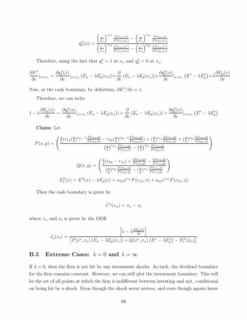
qλ2 (x) =

(

xxu

)r1λ F (r1λ,x)F (r1λ,xu)

−(

xxu

)r2λ F (r2λ,x)F (r2λ,xu)

(

x∗

xu

)r1λ F (r1λ,x∗)F (r1λ,xu)

−(

x∗

xu

)r2λ F (r2λ,x∗)F (r2λ,xu)

Therefore, using the fact that qλ1 = 1 at xu and qλ2 = 0 at xu,

∂Eλ

∂c|x=xu

=∂qλ1 (x)

∂c|x=xu

(Eu − λEp(xu))+∂

∂c(Eu − λEp(xu))+

∂qλ2 (x)

∂c|x=xu

(

E∗ − λE∗p

)

+λ∂Ep(x)

∂c

Now, at the cash boundary, by definition, ∂Eλ/∂c = 1.

Therefore, we can write

1− λ∂Ep(x)

∂c=

∂qλ1 (x)

∂c|x=xu

(Eu − λEp(xu)) +∂

∂c(Eu − λEp(xu)) +

∂qλ2 (x)

∂c|x=xu

(

E∗ − λE∗p

)

Claim: Let

P (x, y) =

(

1x(r1λ(

y

x)r1λ−1 F (r1λ,y)

F (r1λ,x)− r2λ(

y

x)r2λ−1 F (r2λ,y)

F (r2λ,x)) + ( y

x)r1λ G(r1λ,y)

F (r1λ,x)+ ( y

x)r2λ G(r2λ,y)

F (r2λ,x)(

y

x

)r1λ F (r1λ,y)F (r1λ,x)

−(

y

x

)r2λ F (r2λ,y)F (r2λ,x)

)

Q(x, y) =

(

1y(r2λ − r1λ) +

G(r2λ,y)F (r2λ,y)

− G(r1λ,y)F (r1λ,y)

(xy)r2λ F (r2λ,x)

F (r2λ,y)− (x

y)r1λ F (r1λ,x)

F (r1λ,y)

)

Eλ1 (x) = Eλ(x)− λEp(x) = a1λx

r1λF (r1λ, x) + a2λxr2λF (r2λ, x)

Then the cash boundary is given by

Cλ(xu) = xu − xℓ

where xu and xℓ is given by the ODE

x′u(xℓ) =

[

1− λ∂Ep(x)

∂c

]

[

P (x∗, xu) (Eu − λEp(xu)) +Q(x∗, xu)(

E∗ − λE∗p

)

− Eλ′

1 (xu)]

B.3 Extreme Cases: λ = 0 and λ = ∞

If λ = 0, then the firm is not hit by any investment shocks. As such, the dividend boundary

for the firm remains constant. However, we can still plot the investment boundary. This will

be the set of all points at which the firm is indifferent between investing and not, conditional

on being hit by a shock. Even though the shock never arrives, and even though agents know

66

this, the investment boundary still exists and can be studied. Of course, by continuity, this

case can also be studied as a proxy for the case when λ is vanishingly small.

In this case, it is not hard to show that the smooth pasting condition is always satisfied,

so the only condition that determines the investment boundary curve is the value matching

condition. In particular, the investment boundary curve ℓI is the set of all points x∗ where

E(x∗, c∗) = EH(x∗, c∗−I). As expected, I observe that c∗ decreases as x∗ increases, implying

that firms with more capital can invest holding less liquidity. Therefore, all else being equal,

it is more likely for a firm with a higher amount of capital to invest. This also implies that

when capital falls below a threshold, firms hold liquidity purely for precautionary purposes

and never fund investment - even if they have the opportunity to do so.

When λ = ∞, it corresponds to the case when the firm has the real option in hand.

Again, as Figure 3 shows, the investment boundary curve is a decreasing function of the

firm’s capital stock. However, this is only under the assumption that the firm finances

investment purely out of internal funds. If the firm issues equity while investing, the level

of cash below which the firm invests (by issuing equity) is actually an increasing function of

firm capital. Intuitively, as the level of capital for the firm increases, the real option becomes

more valuable, so it is more willing to incur external finance costs to exercise it.

B.4 Code Methodology:

To simultaneously generate both the cash boundary Cλ(xu) and the investment boundary

ℓI , I proceed in the following steps.

1. First obtain x∗ using the conditions detailed in section 1.5.

2. Impose smooth pasting at x∗ to obtain Cλ′(x∗) and x′

u(xℓ) at x∗.

3. Set a small ǫ > 0. Obtain xnewu = xu + x′

u(xℓ)ǫ. xnewℓ = xℓ + ǫ.

4. Obtain x∗,new by solving the smooth pasting condition (detailed in section 1.4) at x∗.

I use an optimization algorithm for this.

5. Again obtain x′u(xℓ) using x∗,new, xnew

ℓ and xnewu .

6. Go back to step 3.

67

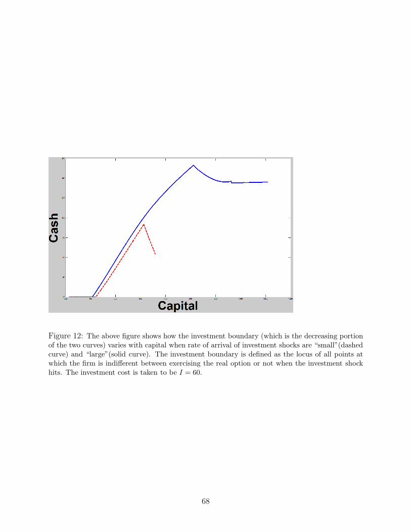
Figure 12: The above figure shows how the investment boundary (which is the decreasing portionof the two curves) varies with capital when rate of arrival of investment shocks are “small”(dashedcurve) and “large”(solid curve). The investment boundary is defined as the locus of all points atwhich the firm is indifferent between exercising the real option or not when the investment shockhits. The investment cost is taken to be I = 60.

68