A Theory of Stability in Dynamic MatchingMarkets

Laura Doval*†

J M P ‡

November 11, 2015

AbstractI study dynamic matching markets where matching opportunities arrive over time, and match-

ing is one-to-one and irreversible. The proposed stability notion, dynamic stability, incorpo-rates a backward induction notion to an otherwise cooperative model, which takes into accountthe time at which the arriving agents can form binding agreements. Dynamically stable match-ings may fail to exist in two-sided economies (e.g., adoption markets), and in the allocation ofobjects with priorities (e.g., public housing). However, dynamically stable matchings alwaysexist in one-sided economies (e.g., deceased-donor organ allocation). The non-existence resultreveals a new form of unraveling in matching markets: agents wish to delay the time at whichthey are matched so as to improve their matching prospects. These findings rationalize whyclearing houses in different markets adopt very different rules to deal with the event in whichagents reject a current offer to wait for a be er match. In particular, in two-sided markets andin the allocation of objects with priorities, to guarantee that efficiency is achieved, the centralclearing house needs to restrict agents’ option to wait for a be er match.

*I am indebted to Eddie Dekel and Jeff Ely for many fruitful conversations and for their continuingguidance and support. I am very thankful to Alessandro Pavan for useful discussions and his detailedcomments. I also wish to thank Hector Chade, Federico Echenique, Pablo Schenone, Asher Wolinsky,Leeat Yariv, and Charles Zheng. All errors are my own.

†Ph.D. Candidate in Economics, Department of Economics, Northwestern University, IL 60208. (e-mail: laura.doval@u.northwestern.edu)

‡Please click here for the latest version.

1

₁ I

Matching markets such as adoption markets, the allocation of public housing, anddeceased-donor organ allocation share the following key features: (i) matching is one-to-one, (ii) matching opportunities arrive over time, and (iii) matching is irreversible.For example, in the case of deceased-donor kidney allocation (i) each patient receivesone kidney, (ii) patients and kidneys arrive into the system at various points in time,and (iii) once a patient is transplanted a kidney, she permanently exits the market.Moreover, for each of these markets, a central clearing house exists: adoption agen-cies manage adoptions, the Public Housing Authority (PHA) manages the allocationof public housing, and the United Network for Organ Sharing (UNOS) manages theallocation of deceased-donor organs.

Since matching opportunities arrive over time, and matching is irreversible, in thesemarkets the option of waiting for a be er match is valuable. For instance, supposeUNOS offers Alex, a 20-year-old patient, a kidney from a 65-year-old deceased-donor.On dyalisis alone, Alex could maintain her current quality of life for up to 4 years (seeSchold et al. [44]). Because matching opportunities arrive over time, Alex understandsthat within the next 4 years, a kidney from a younger deceased-donor may arrive. Suchkidneys are more desirable than the currently offered kidney. Therefore, Alex facesthe following dynamic problem. On the one hand, she could take now the 65-year-olddeceased-donor kidney. If she does this, because matching is irreversible, she quits themarket and misses out on the option of receiving the younger kidney within the next4 years. On the other hand, at the cost of giving up her current offer, she may wantto keep her options open, and wait for a younger deceased-donor organ to enter thesystem. Alex’s ultimate decision will depend on how she weighs the pros and cons ofwaiting versus matching immediately.

Despite their similarities, which imply that in all these markets the option of wait-ing for a be er match is valuable, the clearing houses through which matches occurdiffer greatly in how they deal with the event in which an agent is proposed a match,but turns it down to wait for a be er prospect. In adoption markets, once a matchbetween an adoptive parent and a birth mother is proposed, adoption agencies allowbirth mothers to costlessly renege on the match. In contrast, depending on the agency,adoptive parents face different restrictions after reneging on the match: for example,restarting the process within the agency, having to proceed with adoption with a dif-ferent agency, or being placed at the bo om of the agency’s wait list. The PHA [35]establishes that if an applicant rejects an offer to match with a compatible building to-day, then she is either removed from the waiting list, and has to restart her application,

2

or she is placed at the bo om of the waiting list with a new application date. In con-trast, if a patient refuses to match with a compatible kidney, UNOS does not penalizethe patient in any way.

This paper provides a theory of stability in dynamic matching markets that satisfyproperties (i)-(iii) above. Stability notions are used to predict which arrangementsagents reach in a laissez-faire situation. Since stable outcomes are Pareto efficient,whenever they exist, even in the absence of central clearing houses, one expects ex-changes to be efficient. Thus, while clearing houses may exist to facilitate other aspectsof the matching market, they need not regulate the actions that agents can take for thepurpose of achieving efficiency: agents themselves will naturally reach a stable, andthus efficient, allocation.

This paper makes two contributions. First, it provides a framework that rationalizeswhy, across the above three markets, the institutional rules that regulate what happenswhen agents wait for a be er match are so different, even though similar forces drivethe incentive to wait for a be er match in all three. Second, I use the framework to un-derstand when, to guarantee efficiency, a central clearing house is needed to regulatethe actions agents can take.

In order to do so, I proceed in three steps. First, while markets with properties (i)-(iii)above have been studied in the literature, none of the existing papers provide stabil-ity notions. Therefore, I define a stability notion which is natural for such markets. Idenote it dynamic stability. Second, I show that for markets such as adoption marketsand public housing, dynamically stable matchings may fail to exist. This non-existenceproblem arises precisely because agents have the option to wait for be er matching op-portunities. In contrast, in markets such as the allocation of deceased-donor organs,dynamically stable matchings always exist. It follows from these two observations that,in the first two markets, a central clearing house which regulates agents’ actions afterthey decide to reject a current offer to match is needed to guarantee that the allocationis efficient. Third, in markets such as adoption markets and public housing, I providesufficient conditions under which dynamically stable matchings exist. Hence, underthese conditions, a clearing house need not restrict agents’ actions in order to guaranteeefficiency.

1.1 Overview of model

In this section, I present the four key components of the environment. First, I brieflydescribe the model. Second, I define matchings in a dynamic se ing. Third, I discusshow different assumptions on the timing at which agents can form binding agreements

3

determine what a feasible block is. Finally, I use the definitions of a matching and afeasible block to define the two stability notions I consider in this paper.

I consider a stylized model that captures features (i)-(iii) mentioned before. The econ-omy lasts for two periods, and there are two sides, A (adoptive parents in adoptionmarkets, applicants in public housing, ailing patients in the allocation of organs), andB (resp., birth mothers, buildings, body parts). Agents on side A arrive in period 1,while agents on side B arrive (stochastically) over time. Matching is one-to-one, andirreversible. Agents on side A are discounted expected utility maximizers. For agentson side B, I consider three different assumptions to accommodate the different appli-cations of the model: (1) in the two-sided economy, agents on side B are also discountedexpected utility maximizers, (2) in the allocation of objects with priorities, agents on sideB are endowed with strict atemporal rankings over agents on side A, and (3) in theone-sided economy, agents on side B are objects with no preferences over agents on sideA. (The nomenclature follows the one in Abdulkadiroğlu and Sönmez [2].)

In these dynamic environments, a matching should be defined as a complete contin-gent plan (henceforth, contingent matching). It should specify (1) what matches occurin period 1, and (2) for every set of agents that are unmatched at the beginning of pe-riod 2, what matches occur in period 2. In particular, if an agent is supposed to bematched in period 1, the matching also prescribes what her period 2 outcome is, if shedecides instead to remain unmatched. This information is relevant for her decision tocarry through or not the matching prescribed in period 1.

Because the environment is dynamic, one has to be careful when defining what afeasible block is. Consider the following example. Ariel, Anna, and Bob are presentin period 1. Brad arrives in the market in period 2. Suppose Anna is prescribed tomatch with Bob in period 1. The following is an a priori feasible agreement betweenAnna and Brad. (Notice that I am only dealing with feasibility, regardless of whetherthis is optimal for the agents.) In period 1, Anna and Brad can agree, in advance, thatAnna waits for Brad to arrive, and they match in period 2, i.e., they agree that they willmatch in period 2, regardless of Brad’s possibility of matching with Ariel in period 2.In some applications, assuming that Anna and Brad can make this agreement in period1, when Brad is not yet in the market, might be a realistic assumption, while in otherapplications it might not. Depending on the stance one takes with respect to the fea-sibility of such agreements, one obtains different notions of what a feasible blockingcoalition is. In turn, different notions of what a feasible blocking coalition is determinedifferent stability notions. In the stability notions I present below, I consider the twopolar cases: either agents can form binding agreements regardless of when they enterin the market, or agents are only allowed to form binding agreements with their con-

4

temporaries.The first stability notion, the core, allows agents to make agreements amongst them-

selves regardless of when they enter the market (Definition 4.10). A contingent match-ing is in the core if it satisfies the following. There is no subset of agents, regardlessof whether they are contemporary or not, that can propose an alternative matchingamongst themselves with the property that every agent within the subset is be er offunder the alternative matching than under the original one. Since this is the naturalextension of the core from static se ings to the dynamic se ing, core matchings areused as benchmarks throughout the paper.

The second stability notion, dynamic stability, only allows agents to form agreementswith their contemporaries (Definition 4.4). In words, a contingent matching is dynami-cally stable if, for each possible outcome in period 1, the matching among the remainingagents and the new entrants is a stable matching, and, taking as given the outcomesexpected for period 2, there is no group of agents in period 1 who finds it profitable tochange the period 1matching, either by waiting to match in period 2, by changing whothey are matched to in period 1, or both. In the example above, if Anna prefers Brad toBob, and Brad prefers Anna to Ariel, then any dynamically stable contingent match-ing should specify that, if no agent matches in period 1, then Anna and Brad shouldmatch in period 2. Hence, a contingent matching that matches Anna and Bob in period1 cannot be dynamically stable: Anna can change the period 1 outcome by decidingto remain unmatched in period 1, and match with Brad in period 2 as prescribed bythe contingent matching. In this case, the prediction made by the core and dynamicstability coincide. While the matching outcome is ultimately the same, the blocks thatfacilitate this matching are different: in the core, Anna and Brad agree in period 1 tomatch in period 2; in dynamic stability, Anna waits to be matched in period 2, and anystable matching in period 2 matches Anna and Brad together.

The two stability notions, the core and dynamic stability, defined above for two-sidedeconomies, are extended to the allocation of objects with priorities (Definition 4.6), andthe one-sided economy (Definition 4.9).

1.2 Overview of results

In two-sided economies, absent any restrictions on agents’ preferences, dynamicallystable matchings may fail to exist because agents who match in period 1 may improvetheir matching outcome by waiting to be matched in period 2, once certain agents leavethe market (Propositions 5.1 and A.1). An agent’s ability to know she can improve hermatching outcome by waiting depends, in part, on the observability of everyone else’s

5

matching outcomes. It follows from the connection between two-sided markets andthe allocation of objects with priorities, explained in Section 4.1, that the non-existenceresults translate to this case as well. In contrast to the above results, dynamically stablecontingent matchings always exist in one-sided economies. Propositions 5.2-9.1 showthat, in one-sided economies, any Pareto efficient matching is part of a dynamicallystable matching. (Section 5 discusses the intuition behind the results.)

The observation that dynamically stable matchings may fail to exist, absent any re-strictions on agents’ preferences, motivates the sufficient conditions for existence. Ifagents are sufficiently patient dynamically stable matchings exist (Proposition 6.2 inthe case of deterministic arrivals, and 10.3 in the case of stochastic). Alternatively, ifpreferences over matchings across different agents are sufficiently aligned, then dynam-ically stable matchings also exist (Propositions 6.3-6.4 when arrivals are deterministic,and Proposition 10.4 when they are stochastic). Each of these conditions imply thatthere are core matchings which are dynamically stable. Thus, under these conditions,core matchings can be obtained as part of a stability notion that makes less stringentassumptions on the binding agreements available to the agents. It follows from theconnection between two-sided markets and the allocation of objects with priorities thatsimilar, but weaker, conditions guarantee existence (see Sections 6.3-10.3).

The second observation (the possibility of improving one’s outcome by waiting whenobserving everyone else’s matches) motivates the definition of a weaker stability no-tion, correlated dynamic stability (Section 11). In correlated dynamic stability, in anygiven period, each agent is only informed of whom she is matched with that period, orif she is single, but not of next period’s outcome. Since an agent is not informed of otheragents’ matches, unraveling may be precluded by introducing uncertainty about thebenefits of waiting to be matched. Correlated dynamically stable matchings may ex-ist even when dynamically stable do not (Proposition 11.1). However, that correlateddynamically stable matchings may not exist shows that the observability of matchingoutcomes is not the only force at play in the non-existence results (Proposition 11.2).

Finally, I also show that when arrivals are stochastic and agents discount the future,the core may be empty. This is in contrast to the case of deterministic arrivals in which itis always non-empty (Sections 6.1-10.1). When arrivals are stochastic, from an ex-antepoint of view, agents are matched to a set of agents on the other side of the market(potentially one for each arrival realization). If agents discount the future, preferencesmay exhibit complementarities: how valuable matching with an agent at one partic-ular realization is depends on who else is available to match at other realizations. Itis well-known in static many-to-many matching that complementarities preclude ex-istence (Kelso and Crawford [25]); however, the observation that discounting coupled

6

with the stochasticity of the arrivals is a source of complementarities is new. To keepthe discussion focused on the issues pertaining the dynamics of the problem, the fullanalysis of the core when arrivals are stochastic is provided in a companion paper [15].

The above results help us distinguish between two types of economies. First, economieswhere, for the purposes of guaranteeing efficient outcomes, a central planner needs toeither limit the ability of an agent to wait for a be er match, or enforce punishmentsthat dissuade agents from waiting to match. This rationalizes why the PHA expelsagents from the waiting list after rejecting an offer to match with a compatible house.Absent any assumptions on preferences, if the PHA did not impose these punishmentsthe market could unravel. Second, in one-sided markets and in two-sided economieswhere the restrictions on preferences hold, dynamically stable matchings always exist.This acts as a rationale for why UNOS does not punish agents for rejecting a currentmatch: in these economies, the clearing house need not restrict agents’ actions in orderto guarantee efficient allocations are achieved.1

The paper contributes mainly to two strands of literature, which are reviewed inSection 12. The first strand, like here, studies stability notions; however, they applyto markets where matching opportunities are fixed, and pairings can be revised overtime (e.g., Damiano and Lam [13], Kurino [29]). The contribution relative to this strandis to provide stability notions for markets with features (i)-(iii). The second strand isthe algorithm/mechanism design literature which studies, like here, markets with fea-tures (i)-(iii), but from the point of view of optimality, instead of stability (Ünver [48],Leshno [31], Akbarpour et al. [3], Baccara et al. [6]). The present study of stability isimportant because stability is considered a key property for the success of algorithms(Roth [39]), and because it identifies a new form of unraveling due to agents waitingfor be er matching opportunities.

The rest of the paper is organized as follows. Section 2 introduces the core and dy-namic stability by means of an example which highlights the limitations of the corewhen thinking about dynamic matching markets; it also discusses the implications ofthe theory for list kidney exchange. The reader interested in the definitions may skipthese, and go directly to Section 3, where the model and notation are introduced, andSection 4 where the stability notions are defined. For ease of exposition, Sections 3-6deal with the case in which arrivals are deterministic. Section 5 contains the (non-)existence results. Section 6 analyzes sufficient conditions on preferences under whichdynamically stable matchings exist in two-sided economies, and the allocation of ob-

1I address in Remark 10.3 how the allocation of deceased-donor kidneys can be modeled as theallocation of objects with priorities in a way such that existence is guaranteed. Hence, the core messageof the paper remains true: UNOS need not limit agents’ option to wait to achieve efficiency. Here, Ifollow the literature in modeling the allocation of kidneys as a one-sided economy.

7

jects with priorities. Sections 7-10 deal with the case of stochastic arrivals, mirroringthe presentation in Sections 3-6. Section 11 defines correlated dynamic stability, anddiscusses how randomization may be used to partially restore existence. Section 12discusses extensions, and the relevant literature. Section 13 concludes.

₂ E : C . D S

Example 2.1 below highlights the differences between the core and dynamic stability:

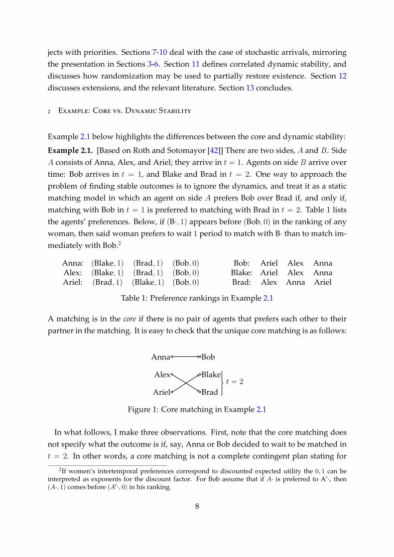
Example 2.1. [Based on Roth and Sotomayor [42]] There are two sides, A and B. SideA consists of Anna, Alex, and Ariel; they arrive in t = 1. Agents on side B arrive overtime: Bob arrives in t = 1, and Blake and Brad in t = 2. One way to approach theproblem of finding stable outcomes is to ignore the dynamics, and treat it as a staticmatching model in which an agent on side A prefers Bob over Brad if, and only if,matching with Bob in t = 1 is preferred to matching with Brad in t = 2. Table 1 liststhe agents’ preferences. Below, if (B·, 1) appears before (Bob, 0) in the ranking of anywoman, then said woman prefers to wait 1 period to match with B· than to match im-mediately with Bob.2

Anna: (Blake, 1) (Brad, 1) (Bob, 0) Bob: Ariel Alex AnnaAlex: (Blake, 1) (Brad, 1) (Bob, 0) Blake: Ariel Alex AnnaAriel: (Brad, 1) (Blake, 1) (Bob, 0) Brad: Alex Anna Ariel

Table 1: Preference rankings in Example 2.1

A matching is in the core if there is no pair of agents that prefers each other to theirpartner in the matching. It is easy to check that the unique core matching is as follows:

Anna Bob

Alex Blake

Ariel Bradt = 2

Figure 1: Core matching in Example 2.1

In what follows, I make three observations. First, note that the core matching doesnot specify what the outcome is if, say, Anna or Bob decided to wait to be matched int = 2. In other words, a core matching is not a complete contingent plan stating for

2If women’s intertemporal preferences correspond to discounted expected utility the 0, 1 can beinterpreted as exponents for the discount factor. For Bob assume that if A· is preferred to A′·, then(A·, 1) comes before (A′·, 0) in his ranking.

8

each possible outcome in t = 1 what matching will ensue in t = 2. If waiting to bematched is an option for the agents, this should be specified.

Second, complete contingent plans should specify credible “off-path” outcomes. Inturn, whether the “off-path” outcomes are credible or not depends on the bindingagreements agents can form amongst themselves. Notice that, in t = 2, the remain-ing unmatched agents form a static matching market. Hence, in line with the rest ofthe matching literature, I assume agents can form binding agreements with their con-temporaries. Hence, no agent should expect that a non-stable matching will arise int = 2, making stable matchings the only reasonable “off-path” outcomes.

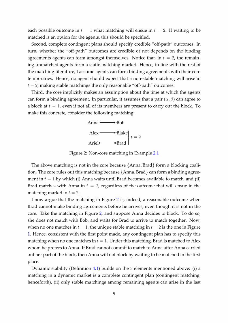
Third, the core implicitly makes an assumption about the time at which the agentscan form a binding agreement. In particular, it assumes that a pair (α, β) can agree toa block at t = 1, even if not all of its members are present to carry out the block. Tomake this concrete, consider the following matching:

Anna Bob

Alex Blake

Ariel Bradt = 2

Figure 2: Non-core matching in Example 2.1

The above matching is not in the core because {Anna,Brad} form a blocking coali-tion. The core rules out this matching because {Anna,Brad} can form a binding agree-ment in t = 1 by which (i) Anna waits until Brad becomes available to match, and (ii)Brad matches with Anna in t = 2, regardless of the outcome that will ensue in thematching market in t = 2.

I now argue that the matching in Figure 2 is, indeed, a reasonable outcome whenBrad cannot make binding agreements before he arrives, even though it is not in thecore. Take the matching in Figure 2, and suppose Anna decides to block. To do so,she does not match with Bob, and waits for Brad to arrive to match together. Now,when no one matches in t = 1, the unique stable matching in t = 2 is the one in Figure1. Hence, consistent with the first point made, any contingent plan has to specify thismatching when no one matches in t = 1. Under this matching, Brad is matched to Alexwhom he prefers to Anna. If Brad cannot commit to match to Anna after Anna carriedout her part of the block, then Anna will not block by waiting to be matched in the firstplace.

Dynamic stability (Definition 4.1) builds on the 3 elements mentioned above: (i) amatching in a dynamic market is a complete contingent plan (contingent matching,henceforth), (ii) only stable matchings among remaining agents can arise in the last

9

period, and (iii) agents can only “block” (that is, agree to match with an agent on theother side of the market) after they have arrived. In words, in a two-period economy,a contingent matching is dynamically stable if, for each possible outcome in t = 1, thematching among remaining agents and the new entrants is a stable matching, and, tak-ing as given the outcomes expected for t = 2, there is no group of agents in t = 1 thatcan find it profitable to change the matching in t = 1, either by waiting to match int = 2, by changing who they are matched to in t = 1, or both.

For the economy presented in the example, both matchings are dynamically stable.3

In this economy, the set of dynamically stable matchings is a superset of the core.Hence, an outside observer may mistakenly rule out the matching in Figure 2 by usingthe wrong stability notion.

2.1 Implications for list kidney exchange.

Agents’ incentives to wait to improve on their matching outcomes are particularly per-vasive in deceased-donor organ allocation (Su and Zenios [46]). The following stylizedexample illustrates how list kidney exchange in the New England Kidney ExchangeProgram determines an agent’s continuation matching after refusing to be transplantedan organ, and generates incentives for agents to wait, therefore undermining the mech-anism’s ability to implement some efficient matchings.

Example 2.2. There are three patients Anna, Ariel, and Alex. Anna and Ariel are in thelist for deceased-donor transplants. Ariel and Alex are blood type B, Anna is AB. Alexhas a donor with blood typeAB, and hence cannot be transplanted her donor’s kidney.This period one deceased-donor kidney of blood type B, β1, is available, though it isfrom an older patient; next period another blood type B kidney will become available,β2. Both Alex and Ariel prefer to wait for β2, than to be matched this period to β1, andprefer the la er to being unmatched. Assume deceased-donor kidneys expire: if theyare not allocated the period they arrive, they lose their viability. The following alloca-tion is Pareto efficient: Alex donates her donor’s kidney to agent Anna, Alex receivesβ1, Ariel receives β2. Moreover, this is allowed for by list exchange: the incompatiblepatient takes the recipient’s place in the waiting list, and obtains right of first refusal(ROFR) for the next ABO identical deceased-donor kidney, and keeps it until she ac-cepts a transplant (see Delmonico et. al [14]).

After Anna receives Alex’s donor’s kidney, Alex is offered β1. However, ROFR im-plies that, by refusing kidney β1, she obtains the right to receive β2 next period. If Alex

3After appropriately specifying the t = 2 matchings for the different t = 1 outcomes - see AppendixF for details

10

and Ariel are located far away from each other, then, after Alex refuses kidney β1, it ex-pires before reaching Ariel, who is left without a transplant. Therefore, ROFR togetherwith the implied consensus that nobody can force a patient to accept a transplant (im-plicit in the fact that Alex will obtain β2 if she refuses β1) imply that the aforementionedPareto efficient allocation can’t be obtained, and as a consequence a patient is left with-out a transplant.

Notice that, by clearly specifying the “implied property rights” over kidneys, a Paretoefficient allocation that respects ROFR can be achieved: allocate Ariel kidney β1, andAlex kidney β2. Clearly specifying “property rights” over the objects is key to show-ing that Pareto efficient allocations are dynamically stable in one-sided economies (seeSection 5.2).

₃ M

The model, definitions, and results are presented in a two-period economy since thissuffices to introduce the main concepts and issues.4 Below, to remove any ambiguityof what I mean by a stochastic arrival, I define the components of the model in the gen-eral case of stochastic arrivals. Section 3.1, then, defines matchings and preferences inthe case of deterministic arrivals. Section 7.1 defines these objects when arrivals arestochastic.

The economy lasts for two periods. There are two sides. Side A consists of a finiteset of agents, A. Agents a ∈ A are referred to as α-agents. They stand for adoptiveparents in adoption markets, applicants in public housing or job markets, ailing pa-tients in the allocation of organs. Side B consists of β-agents, who arrive over time.β−agents have characteristics belonging to a finite set B. They stand for birth mothersin adoption markets, buildings in public housing, businesses in job markets, body partsin the allocation of organs. A stochastic arrival is a distribution over pairs of subsetsof B, the first subset being the agents arriving in t = 1. More precisely, denote by G adistribution on 2B × 2B such that supp G ⊆ {(B1, B2) ∈ 2B × 2B : B1 ∩ B2 = ∅}. Thisimplies that no two β-agents of the same type arrive in different periods; this maintainsthe assumption of strict preferences typical of two-sided matching.5

The model encompasses the case of deterministic arrivals by se ing supp G = {(B1, B2)}for some (B1, B2) ∈ 2B × 2B, B1 ∩B2 = ∅. The rest of this section focuses on this case.

4When relevant, I point out how to apply the conditions in Sections 6-10 for more than two periods.5The assumption is not used in the one-sided economy.

11

3.1 Deterministic arrivals: Matchings and preferences

I define below matchings for this economy. The definitions capture three ingredients.First, a matching specifies who an agent is matched to every period after she/he arrives.Second, matching is one-to-one and irreversible, so once α is matched to β at period t,she continues to be matched to β at all future periods. Third, the focus is on contingentmatchings that specify, for each t = 1 outcome, the matching that ensues in t = 2.

Definition 3.1. A period tmatching is an injective map mt : A∪∪t

τ=1Bτ 7→ A∪∪t

τ=1 Bτ

such that (∀a ∈ A)mt(a) ∈ {a} ∪∪t

τ=1Bτ , and (∀b ∈∪t

τ=1Bτ )mt(b) ∈ A ∪ {b}. Mt

denotes the set of all period t matchings.

Definition 3.2. A pair (m1,m2) ∈ M1 ×M2 is feasible if (∀a ∈ A)m1(a) = a ⇒ m2(a) =

m1(a).6 M denotes the set of feasible matchings.

Having defined what a static matching is, and what are the feasible matchings inthe economy, I define below a contingent matching. A contingent matching µ selectsa period 1 matching, µ(∅), and, for each possible matching in period 1, m1, it selects aperiod 2 matching, µ(m1) ∈M2, such that (m1, µ(m1)) is feasible. Formally,

Definition 3.3. A contingent matching µ is a map:

µ : {∅} ∪M1 7→M1 ∪M2

s.t. µ(∅) ∈M1 and (∀m1 ∈M1)µ(m1) ∈M2 ∧ (m1, µ(m1)) is feasible.

LetM denote the set of contingent matchings.

Any contingent matching defines how agents match “on-path”, i.e. what matchingensues when all agents match according to what is prescribed by µ:

Definition 3.4. Given µ ∈ M, the on-path matching for µ is the feasible matching mµ =

(m1,µ,m2,µ) ∈M defined as follows:

m1,µ = µ(∅),

m2,µ = µ(µ(∅)).

To complete the definition of the economy, I define each agent’s preferences over (on-path) matchings. I assume agents on side A are discounted utility maximizers. Thatis, for each a ∈ A, assume there exists a Bernoulli utility function u(a, ·) : B 7→ R, anda discount factor δa ∈ [0, 1], such that a’s utility of matching with b at time t is given byδtau(a, b). Assume u(a, a) = 0. In general, given an on-path matching m ∈M , a’s utility

6Since m2 is injective, this automatically implies that m2(m1(a)) = a.

12

from matching m is given by:

U(a,m) = δ1[m1(a)=a]a u(a,m2(a)).

Since matching is irreversible, a’s partner under m is given by m2(a). If a is unmatchedin t = 1, then a obtains the discounted payoff from matching with m2(a) in t = 2.

For two-sided economies, I assume agents on side B are also discounted utility max-imizers. That is, for each b ∈ B, there exists a Bernoulli utility function v(·, b) : A 7→ R,and a discount factor δb ∈ [0, 1]. Assume v(b, b) = 0. For b ∈ B1, his utility frommatching m ∈M is given by:

V1(b,m) = δ1[m1(b)=b]b v(m2(b), b),

and, for b ∈ B2, his utility from matching m is given by:

V2(b,m) = v(m2(b), b).

For the allocation of objects with priorities, I assume (buildings) b ∈ B have a com-plete and transitive binary relation ▷b ⊂ A×A. I extend ▷ to an (incomplete) order overmatchings as follows. Fix b ∈ B1. In what follows, say a ⊵b a

′ if a = a′, or a ▷b a′. Let

m,m′ ∈ M,m = m′. If m1(b) = b, then b prefers m to m′ if, and only if, m1(b) ⊵b m′2(b).

That is, b prefers to match with m1(b) if either m1(b) is at least as good as m′2(b).

Finally, in the one-sided economy, to make the presentation of the definitions in Sec-tion 4.1 homogeneous, one can specify “trivial” preferences for b ∈ B, so that b prefersto be matched over being unmatched. Fix B1 ⊆ B. For b ∈ B1, and m ∈ M(B1), hisutility from matching m is given by:

V1(b,m) =

{0 if m2(b) = b

1 otherwise,

and, for b ∈ B2, his utility from matching m is given by:

V2(b,m) =

{0 if m2(b) = b

1 otherwise.

The tuple E = ⟨A,B, G, {δa, u(a, b)}a∈A, {δb, v(a, b)}b∈B,M⟩defines the two-sided econ-omy, EB,▷ = ⟨A,B, G, {δa, u(a, b)}a∈A, {▷b}b∈B,M⟩ defines the allocation of objects withpriorities, and EB = ⟨A,B, G, {δa, u(a, b)}a∈A,M⟩ defines the one-sided economy.

13

₄ S

4.1 Dynamic Stability

In this section, I define dynamic stability. I do so first, for two-sided economies, then,for the allocation of objects with priorities, and, finally, for one-sided economies.

Fix a matching µ ∈M, and a period 1 matching, m1. Let

A(m1) = {a ∈ A : m1(a) = a},

B(m1) = {b ∈ B1 : m1(b) = b} ∪ B2,

denote the unmatched agents at the beginning of period 2, when in period 1 agentsmatched according to m1. For all purposes ⟨A(m1),B(m1)⟩ is a static matching market.Hence, the definition of a block atm1 (Definition 4.2) coincides with the standard notionin static matching markets. Definition 4.2 states that only agents inA(m1)∪B(m1) mayblock µ(m1) (all other agents have matched in t = 1), and these blocks are subject totwo restrictions (Definition 4.1): (1) any new matches have to be amongst membersof the coalition, and (2) if a match is broken as a consequence of the block, one of theagents involved in the broken match is part of the block.

Definition 4.1. Fix a (static) matchingm : A∪B 7→ A∪B. Coalition ∅ = A′∪B′ ⊆ A∪Bcan enforcem′ over m if (∀k ∈ A′ ∪B′):

1. m′(k) /∈ {k,m(k)} ⇒ {k,m′(k)} ⊂ A′ ∪B′,

2. m′(k) = k = m(k)⇒ {k,m(k)} ∩ (A′ ∪B′) = ∅.

Definition 4.2. Fix µ ∈ M, and a period 1 matching m1 ∈ M1. ⟨A′, B′,m′⟩ is a block ofµ atm1 if:

1. A′ ∪B′ ⊂ A(m1) ∪ B(m1) can enforce m′ over µ(m1),

2. (∀a ∈ A′)u(a,m′(a)) > u(a, µ(m1)(a)), and

3. (∀b ∈ B′)v(m′(b), b) > v(µ(m1)(b), b).

Definition 4.3 states what a feasible blocking coalition in period 1 is. First, it can onlyconsist of agents in A ∪ B1. Second, in period 1, a coalition can propose a new con-tingent matching that (a) can alter the matchings planned for period 1, (b) cannot alterthe matchings planned for t = 2,m1 ∈ M1. Part (b) is based on backwards induction:a coalition A′ ∪ B′ takes as given the matchings that will occur for each possible out-come in period 1, that is, it holds {µ(m1)}m1∈M1 fixed. However, A′ ∪ B′ may alter the

14

matching at period 1, µ(∅), which determines which m1 realizes in the last period, andhence which µ(m1).

Definition 4.3. Fix µ ∈M. ⟨A′, B′, µ′⟩, is a block of µ at t = 1 if:

1. A′ ∪B′ ⊆ A ∪B1 can enforce µ′(∅) over µ(∅),

2. (∀m1 ∈M1)µ′(m1) = µ(m1),

3. (∀a ∈ A′)U(a,mµ′) > U(a,mµ), and

4. (∀b ∈ B′)V1(b,mµ′) > V1(b,mµ).

Definition 4.4. A contingent matching µ is dynamically stable if it has no blocks at t = 1,and (∀m1 ∈ M1) it has no blocks at m1. D(E) denotes the set of dynamically stablematchings.

Remark 4.1. In independent and contemporaneous work, Kadam and Kotowski [22]define ”dynamic stability” for a two-period matching model in which the set of agentsis constant over time but pairings can be revised as time passes. Not only the se ingof both models differs, but their definition of dynamic stability applies only to on-pathmatchings (i.e. to elements of M in my model), while the concept studied here appliesto contingent matchings (i.e. to elements ofM).

In static allocation of objects with priorities, the stability notion used is elimination ofjustified envy: if a ∈ A prefers b ∈ B to her match, then b is assigned to an agent withhigher priority for b than a. Balinski and Sönmez [7] show that any matching that elim-inates justified envy corresponds to a stable matching in a two-sided economy whereobjects’ priorities are regarded as preferences. In the same spirit, I extend dynamicstability to dynamic elimination of justified envy by using objects’ priorities, and thederived order over M , discussed in Section 3.1, in Definitions 4.2-4.3. In order to doso, I first modify the definition of what matchings a blocking coalition can enforce: inparticular, buildings do not “break up” with applicants to remain single.

Definition 4.5. Fix a (static) matchingm : A∪B 7→ A∪B. Coalition ∅ = A′∪B′ ⊆ A∪Bcan enforcem′ over m if the conditions of Definition 4.1 hold, and:

3∗. b ∈ B′ ⇒ m′(b) = b.

Definition 4.6. Fix µ ∈ M. µ dynamically eliminates justified envy if it has no blocksin period 1, and (∀m1 ∈ M1), it has no blocks at m1, where blocks are defined usingDefinition 4.5. Denote by DNE(EB,▷) the set of contingent matchings that eliminatejustified envy.

Finally, I extend dynamic stability to the one-sided economy. Using the preferences

15

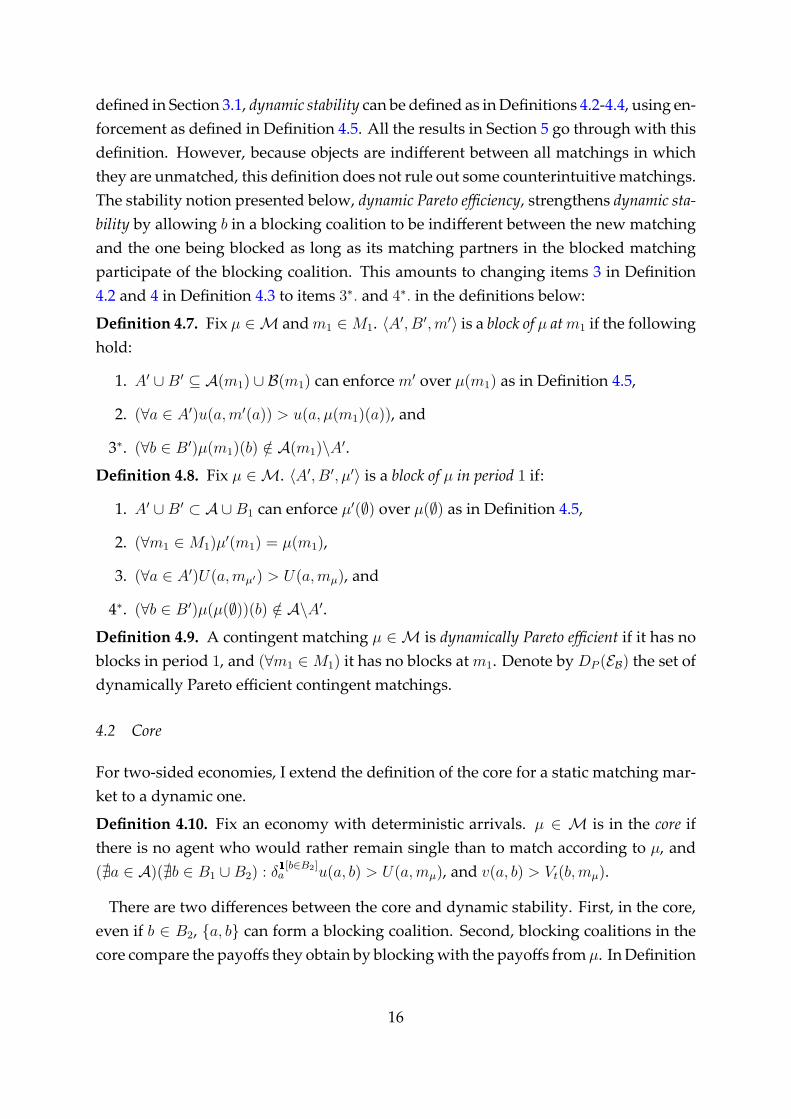
defined in Section 3.1, dynamic stability can be defined as in Definitions 4.2-4.4, using en-forcement as defined in Definition 4.5. All the results in Section 5 go through with thisdefinition. However, because objects are indifferent between all matchings in whichthey are unmatched, this definition does not rule out some counterintuitive matchings.The stability notion presented below, dynamic Pareto efficiency, strengthens dynamic sta-bility by allowing b in a blocking coalition to be indifferent between the new matchingand the one being blocked as long as its matching partners in the blocked matchingparticipate of the blocking coalition. This amounts to changing items 3 in Definition4.2 and 4 in Definition 4.3 to items 3∗. and 4∗. in the definitions below:

Definition 4.7. Fix µ ∈M and m1 ∈M1. ⟨A′, B′,m′⟩ is a block of µ atm1 if the followinghold:

1. A′ ∪B′ ⊆ A(m1) ∪ B(m1) can enforce m′ over µ(m1) as in Definition 4.5,

2. (∀a ∈ A′)u(a,m′(a)) > u(a, µ(m1)(a)), and

3∗. (∀b ∈ B′)µ(m1)(b) /∈ A(m1)\A′.

Definition 4.8. Fix µ ∈M. ⟨A′, B′, µ′⟩ is a block of µ in period 1 if:

1. A′ ∪B′ ⊂ A ∪B1 can enforce µ′(∅) over µ(∅) as in Definition 4.5,

2. (∀m1 ∈M1)µ′(m1) = µ(m1),

3. (∀a ∈ A′)U(a,mµ′) > U(a,mµ), and

4∗. (∀b ∈ B′)µ(µ(∅))(b) /∈ A\A′.

Definition 4.9. A contingent matching µ ∈ M is dynamically Pareto efficient if it has noblocks in period 1, and (∀m1 ∈M1) it has no blocks at m1. Denote by DP (EB) the set ofdynamically Pareto efficient contingent matchings.

4.2 Core

For two-sided economies, I extend the definition of the core for a static matching mar-ket to a dynamic one.

Definition 4.10. Fix an economy with deterministic arrivals. µ ∈ M is in the core ifthere is no agent who would rather remain single than to match according to µ, and(∄a ∈ A)(∄b ∈ B1 ∪B2) : δ

1[b∈B2]a u(a, b) > U(a,mµ), and v(a, b) > Vt(b,mµ).

There are two differences between the core and dynamic stability. First, in the core,even if b ∈ B2, {a, b} can form a blocking coalition. Second, blocking coalitions in thecore compare the payoffs they obtain by blocking with the payoffs from µ. In Definition

16

4.3, a coalition which blocks by waiting in period 1 compares its payoffs at mµ with thepayoffs they obtain at the continuation originated by the block.

In the one-sided economy, the core criterion is Pareto efficiency, as defined below.Pareto efficient matchings are key in the existence results in Section 5.2.

Definition 4.11. An on-path matching m ∈ M is Pareto efficient if there is no otheron-path matching m′ ∈ M such that (∀a ∈ A)U(a,m′) ≥ U(a,m), and (∃a′ ∈ A) :

U(a′,m′) > U(a,m).

₅ D S : E

5.1 Two-sided economies and the allocation of objects with priorities

This section presents the main non-existence result: dynamically stable matchings mayfail to exist in two-sided economies. Since the instance of an economy used to showthis satisfies that no agent on side B blocks by waiting, Proposition 5.1 implies thatDNE may be empty as well.

Proposition 5.1. There exist economies with deterministic arrivals, E , such that D(E) = ∅.

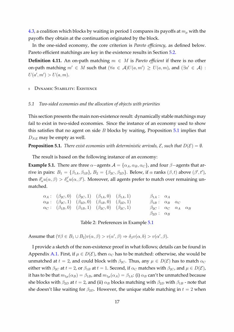
The result is based on the following instance of an economy:

Example 5.1. There are three α−agents A = {αA, αB, αC}, and four β−agents that ar-rive in pairs: B1 = {β1A, β1B}, B2 = {β2C , β2D}. Below, if α ranks (β, t) above (β′, t′),then δtαu(α, β) > δt

′αu(α, β

′). Moreover, all agents prefer to match over remaining un-matched.

αA : (β2C , 0) (β2C , 1) (β1A, 0) (β1A, 1) β1A : αA

αB : (β2C , 1) (β2D, 0) (β1B, 0) (β2D, 1) β1B : αB αC

αC : (β1B, 0) (β1B, 1) (β2C , 0) (β2C , 1) β2C : αC αA αB

β2D : αB

Table 2: Preferences in Example 5.1

Assume that (∀β ∈ B1 ∪B2)v(α, β) > v(α′, β)⇒ δβv(α, b) > v(α′, β).

I provide a sketch of the non-existence proof in what follows; details can be found inAppendix A.1. First, if µ ∈ D(E), then αC has to be matched: otherwise, she would beunmatched at t = 2, and could block with β2C . Thus, any µ ∈ D(E) has to match αC

either with β2C at t = 2, or β1B at t = 1. Second, if αC matches with β2C , and µ ∈ D(E),it has to be that m1µ(αB) = β1B, and m1µ(αA) = β1A: (i) αB can’t be unmatched becauseshe blocks with β2D at t = 2, and (ii) αB blocks matching with β2D with β1B - note thatshe doesn’t like waiting for β2D. However, the unique stable matching in t = 2 when

17

only αA matches with β1A in t = 1, matches αB with β2C , whom she prefers to β1B.Hence, αB has a block against any such µ by waiting. Similar reasoning rules out thatthere exists µ ∈ D(E), and m1,µ(αC) = β1B.

The market unravels, but in a different way than previously emphasized in the litera-ture. Unraveling usually refers to the case in which matches are made too early, like inNational Resident Matching Program (NRMP), as documented by Roth and Xing [43],while here the market unravels because agents want to wait to be matched. This is notmerely a difference in timing. In the NRMP, a procedure which produced unstablematchings was used to determine the matching between residents and hospitals. Thisimplied that there existed gains to be made from blocking, and these were realized bymatching before the market opened. On the contrary, agents in my model expect that astable matching will arise in t = 2 when they wait. Agents who match at t = 1 exit themarket, and, hence, free up matching opportunities in t = 2 for the remaining agents.These are the gains that the agents who block by waiting want to realize. Moreover,these gains can be realized because t = 2 matchings are stable. In Example 5.1, whenαA matches with βA in t = 1, she implicitly gives up her priority with β2C above αB;then, αB can be matched to β2C in a stable matching in t = 2. Thus, the unravelingresult is a consequence of the positive externality agents who match early exert on theremaining agents in the market.7

5.2 One-sided economies

In one-sided economies, dynamically stable matchings always exist:

Proposition 5.2. Fix a one-sided economy, EB. Then, for any Pareto efficient matching m,there exists µ ∈ DP (EB) : mµ = m.

The proof of Proposition 5.2 is in Appendix B. There are two key insights. First, if amatching is Pareto efficient, then there can be no gains from trade amongst agents onside A. In particular, any agent who matches in period 1 has exhausted the value ofthe option to wait for a be er match. This means one can always find period 2 Paretoefficient matchings such that no agent can improve by waiting. However, as illustratedin Example 2.2, not all period 2 Pareto efficient matchings prevent agents from waitingto be matched. The second key insight is the following: a Pareto efficient matching de-

7It is also different from the one in Du and Livne [17], who consider a two-period model in whichα and β−agents arrive over time, and in which a stable matching forms in t = 2, and unraveling as inRoth and Xing occurs. There are many differences between Du and Livne’s model and the one presentedhere, but the different forms of unraveling are not a consequence of the authors considering a setup inwhich α−agents also arrive in t = 2. It is easy to create examples in which there is entry of α−agents int = 2 and the market still unravels forward.

18

termines an “ownership structure” over the objects. If continuation matchings respectsaid “ownership structure”, then no agent has an incentive to wait for a be er match.

I now expand on the second insight. When arrivals are deterministic, just as in staticenvironments, one can show that any Pareto efficient matching has the following prop-erty. There exists an agent who, at the Pareto efficient matching, obtains her most pre-ferred object in B1 ∪ B2. Remove this agent and this object; then, there exists an agentwho, in the Pareto efficient matching, gets her most preferred object out of the remain-ing ones. Repeat this until no agents or objects remain. This gives an ordering of theagents, where the first agent is the one who obtains her most preferred object, the sec-ond agent obtains her most preferred object out of the remaining ones, etc. Hence, anyPareto efficient allocation can be obtained by a serial dictatorship. By prescribing that forall m1, µ(m1) is calculated by respecting the order in the serial dictatorship amongstthe remaining unmatched agents, one guarantees that Pareto efficient matchings aredynamically stable. Recall Example 2.2. Right of first refusal makes the patient whosedonor donated a kidney to someone in the deceased-donor organ waiting list, Alex,the dictator for the ABO compatible deceased-donor kidneys, and hence she obtainsher most preferred ABO compatible kidney. However, the matching suggested in theexample made Ariel the dictator, since she was obtaining her most preferred kidney.

The observation that any Pareto efficient on-path-matching can be obtained as part ofa dynamically Pareto efficient one implies that, in order to achieve efficiency on-path,agents do not need to be promised inefficient matchings “off-path”, i.e. after unex-pected refusals to receive an object. There are two ways to interpret the result. On theone hand, it rationalizes why UNOS does not punish agents after they reject an offer tomatch. On the other hand, if one wishes to remain agnostic about the reasons behindthe mechanism being used to allocated deceased-donor organs, it says that UNOS hasthe potential to implement any Pareto efficient matching without the need of resortingto inefficient punishments “off-path”. The results in this section indicate that, by care-fully designing the waiting lists so as to respect the implicit property rights, in fact,there is no need for such enforcement power. 8

Remark 5.1. [Pareto efficiency in the allocation of objects with priorities] As discussedin Section 4.1, matchings that eliminate justified envy are constructed by looking atthe stable matchings in a two-sided economy where objects’ priorities are regarded aspreferences. In the two-sided economy, stable matchings are always Pareto efficient.However, they need not be Pareto efficient for each side of the market (see Roth [37]).

8Of course, this environment is stylized. In particular, there is no asymmetric information about thequality of the body part an ailing patient is offered. In an ongoing paper, I extend the setup consideredhere to the case in which such asymmetric information exists, and I find that the optimal mechanismalways selects continuations in the Pareto frontier, i.e. it is renegotiation-proof.

19

Thus, matchings which eliminate justified envy need not be Pareto efficient in the al-location of objects with priorities, where Pareto efficiency is defined as in Definition4.11. The economy of Example 5.1 is an instance of this. In particular, the matchingin which m1(αA) = β1A,m1(αB) = β1B and m2(αC) = β2C cannot be improved uponby any pair (α, β) matching together, and thus eliminates (static) justified envy. How-ever, it is not Pareto efficient: αB, αC can improve by exchanging their assigned objects.Moreover, by waiting, αB can trigger this improvement without causing justified envysince αA exits the market in period 1. This tension between efficiency and stability inthe allocation of objects with priorities is important in the non-existence result. Indeed,the sufficient conditions presented in Sections 6.3-10.3 are such that, under these con-ditions, there exists an (on-path) matching which cannot be improved upon by agentsmatching with contemporary objects to which they have priority and is Pareto efficient.The discussion in this section implies that said on-path matching can be made part ofa contingent matching in DNE .

₆ S

Section 6 studies sufficient conditions on preferences under which dynamically stablematchings exist in two-sided economies, and in the allocation of objects with priorities.In particular, under these conditions, there are core matchings which are dynamicallystable. Section 6.1 establishes existence of the core. Sections 6.2 presents the existenceresults for two-sided economies, and Section 6.3 for the allocation of objects with pri-orities.

6.1 Benchmark: Core

When arrivals are deterministic, core contingent matchings always exist:

Proposition 6.1 (Gale and Shapley [21]). Let E be an economy with deterministic arrivals.Then, C(E) = ∅.

Let (B1, B2) denote the arrivals in E . The result follows immediately from applyingGale and Shapley’s algorithm with agents in A proposing, agents in B1 ∪ B2 on thereceiving side, and agent a proposing to b ∈ Bt before proposing to b′ ∈ Bt′ if, and onlyif, δt−1

a u(a, b) > δt′−1a u(a, b′).

In what follows, a subset of C(E) is particularly important: the set of core matchingsthat, for each m1, selects a stable matching for ⟨A(m1),B(m1)⟩. I denote it by C∗(E).Notice that if µ ∈ C(E), there exists µ′ ∈ C∗(E) such that mµ′ = mµ, since blocking

20

coalitions do not take into account the “off-path” matchings specified by µ when de-ciding to block (see Section 4.2).

6.2 Two-sided economies: deterministic arrivals

I present conditions on agents’ preferences that imply that D(E) = ∅. Under theseconditions, C∗(E) ∩ D(E) = ∅. In what follows, I introduce two conditions: almost nodiscounting and no simultaneous cycles. If one or the other is satisfied, then dynamicallystable matchings exist.

Proposition 6.2 below states that if preferences are such that (∀a ∈ A)(∀b, b′ ∈ B)u(a, b′) >u(a, b) ⇒ δau(a, b

′) > u(a, b), then dynamically stable matchings exist. Fix µ ∈ C∗(E).Construct the following µ′ ∈ M. First, mµ′ = mµ. Second, for every t = 2 continua-tion generated by a coalition A′ ∪ B′ ⊆ A ∪ B1 blocking by waiting, let µ′(m1) = m2,µ.Third, for all other m1, set µ′(m1) = µ(m1). The above condition on preferences, whichI denote almost no-discounting, implies that µ′ ∈ C∗(E)∩D(E). In particular, the choiceof µ′(h2) after blocks by waiting is, indeed, a stable match.9

Proposition 6.2. Consider an economy with deterministic arrivals E that satisfies almost nodiscounting. Then, (∀µ ∈ C∗(E))(∃µ′ ∈ D(E)) : mµ′ = mµ.

The proof of Proposition 6.2 is not included in the appendix since it follows imme-diately from the first step in the proof of Proposition 6.3 below. Almost no discountingimplies that, even though agents who match in t = 1 potentially generate incentivesfor other agents to wait to be matched in t = 2, there always exists a stable matching inthe continuation in which the agents who wait do not improve on their current match-ing outcome. Recall Example 5.1: αB does not want to wait for β2D, but when β1B, β2D

are present in the same period, she prefers to match with β2D. This reversal, due todiscounting, implies αB cannot be matched with β1B in t = 2.

The following result, Proposition 6.3, shows that whenever µ ∈ C∗(E)\D(E), thenthere is a simultaneous preference cycle, and motivates the next sufficient condition forexistence. A simultaneous preference cycle (Definition 6.1) is an alternating sequenceof α and β−agents, where every other position is taken by a β−agent, such that: (1)each α−agent prefers the β−agent on her right to the β−agent on her left, and bothβ−agents are acceptable to the α−agent, and (2) each β−agent prefers the α−agent tohis right to the one on his left, and both α−agents are acceptable to the β−agent. Thecycles are evaluated using the t = 1 preferences of α−agents, and the static preferences

9Suppose the economy lasts for T > 2 periods. There is a continuation in period T − 1 such thatno one has matched up to T − 1. Almost no discounting should hold. Recursively, in period T − t, ifu(a, b) > u(a, b′), then δtau(a, b) > u(a, b′).

21

of β−agents since any core, or dynamically stable matching matches a β−agent withan α−agent when he arrives. β−agents’ intertemporal preferences are important todetermine whether a β−agent wants to wait to be matched to an α−agent in t = 2. Inwhat follows, I denote a β−agent of characteristic b that arrives in period t as bt.

Definition 6.1. Fix an economy with deterministic arrivals E . A simultaneous preferencecycle of length N + 1 consists of distinct b0,t0a0, b1,t1 ..., bN,tN , aN such that:

1. (∀n = 0, ..., N)δti+1−1ai u(ai, bi+1,ti+1

) > δti−1ai

u(ai, bi,ti) > u(ai, ai), and

2. (∀n = 0, ..., N)v(ai+1, bi,ti) > v(ai, bi,ti) > v(bi,ti , bi,ti).

where the indices are taken modulo N + 1.10

Notice that the economy in Example 2.1 has a simultaneous cycle with αCβ2CαBβ2B,and the set of dynamically stable allocations is non-empty and encompasses the core.So, a priori, there is nothing ”evil” about preference cycles. However, whenever µ ∈C∗(E)\D(E) there has to be a simultaneous preference cycle.

Proposition 6.3. Fix an economy with deterministic arrivals, E . If µ∗ ∈ C∗(E)\D(E), thereexists at least one simultaneous cycle in E .

The proof is in Appendix C.1. The result is similar in spirit to the DecompositionLemma (Roth and Sotomayor [42]). It follows from comparing the welfare of the two-sides of the market between mµ∗ and mµ′ for some µ′ obtained from µ∗ by a block bywaiting. However, this has to be done with care: since different agents match in t = 2

under µ∗ and µ′, reversals due to discounting have to be considered when compar-ing welfare, while in the Decomposition Lemma preferences are constant across thematchings being compared.

To make the result concrete, recall Example 5.1; there is a simultaneous preference cy-cle (αBβ2CαCβ1B). It can be shown thatm = (m1,m2) such thatm1(αA) = β1A,m1(αB) =

β1B,m1(αC) = αC , and m2(αC) = β2C is an on-path matching for a core matching.Hence, there exists µ ∈ C∗(E) such that mµ = m. Recall from the discussion in Sec-tion 5.1 that αB blocked any such µ by waiting: the unique continuation when αA, β1A

match in t = 1 matches αB with β2C , and αC with β1B in t = 2. Since αB prefers waitingfor β2C over matching with β1B, µ has a block by waiting. Since m is on-path for thecore, it has to be that β2C prefers αC over αB. Moreover, since the t = 2 continuationwhen αA and β1A match in t = 1 is stable, then αC has to prefer β1B over β2C . Finally,

10Romero-Medina and Triossi [36] use the no simultaneous cycles property as a sufficient condi-tion for the core of a many-to-one matching problem with responsive preferences to be unique, andEchenique and Yenmez [19] use a no preference cycle condition in many-to-one matching with prefer-ence over colleagues.

22

since m is on-path for the core, β1B has to prefer αB over αC , thus completing the cycle.

Remark 6.1. The no simultaneous cycle property is implied by the top-coalition prop-erty (Banerjee et al. [9]), and aligned preferences (Nierdele and Yariv [32], Clark [11]).11

Note that since I am not assuming almost no-discounting, these properties have to bechecked using the ex-ante preferences of the agents.12

In Example 5.1, almost no discounting and no simultaneous cycles fail to hold. In-deed, αB prefers β2D over β1B; however, αB prefers to match immediately with β1B towait for β2D. The discussion in the previous paragraph shows there is a simultaneouscycle. Since preferences fail almost no discounting, αB cannot be matched to β1B whenαA matches in period 1, and she waits to be matched in period 2. However, this doesnot mean αB can realize the gain from αA giving up her priority over β2C : this followsfrom the simultaneous cycle, which allows αB to “trade” with αC her priority at β1B inexchange of her priority at β2C .

The absence of simultaneous cycles implies something stronger than just existenceof dynamically stable matchings; it implies that C∗(E) = D(E). This is recorded inProposition 6.4, and proved in Appendix C.2:

Proposition 6.4. Fix E an economy with deterministic arrivals. If E has no simultaneouspreference cycles, then C∗(E) = D(E).

I finish this section by making two remarks:

Remark 6.2 (Singleton blocks by waiting). One could relax Definition 4.3 to allow onlyfor singleton blocks by waiting.13 In that case, no simultaneous cycles can be refined; inparticular, it is enough that there are no simultaneous cycles involving β−agents fromB1 and B2.

Remark 6.3 (One-sided efficiency vs. stability). Recall the discussion in Remark 5.1:the matching µ ∈ C∗(E) such that m1,µ(αA) = β1A, m1,µ(αB) = β1B, and m2,µ(αC) = β2C

is not Pareto efficient. Moreover, by waiting to be matched in period 2, αB triggersa Pareto improvement for agents in A. This observation is more general (see LemmaC.2): when a coalition of α−agents blocks by waiting a core matching, it generates aPareto improvement for α−agents who match in period 2 (same holds for B′ ⊆ B1

blocking a core matching by waiting). However, contrary to the allocation of objectswith priorities, the tension between stability and one-sided efficiency is not the onlyforce at play. One can construct examples in which no individual agent blocks by

11I thank Leeat Yariv for bringing up hers and Clark’s paper to my a ention.12As with almost no discounting, if the economy lasts for T > 2 periods, no simultaneous cycles

should hold at each continuation.13All the non-existence examples presented in the paper only involve blocks by waiting by one agent.

However, one can construct instances in which no single agent blocks by waiting, but a group does.

23

waiting, but a pair (a, b) blocks by waiting, not generating Pareto improvements foreither side. See Appendix S.4.

6.3 Allocation of objects with priorities

I now present sufficient conditions for existence of dynamically stable matchings inthe allocation of objects with priorities. As discussed in Remark 5.1, under these con-ditions, there exists an (on-path) matching which simultaneously eliminates justifiedenvy and is Pareto efficient. Hence, under these conditions, DNE = ∅.

Ergin [20] shows that, when priorities satisfy Ergin-acyclicity, then the matching ob-tained by agents on side A making offers to objects on side B is Pareto efficient andstrategy-proof. In what follows, I define Ergin-acyclicity, and then state the main exis-tence result for the allocation of objects with priorities when arrivals are deterministic:

Definition 6.2. Fix b, b′ ∈ B. {b, b′} form a two-cycle if (∃a, a′, a′′) such that a▷ba′▷ba′′▷b′a.EB,▷ satisfies Ergin-acyclicity if (∀b, b′ ∈ B)b, b′ do not form two-cycles.

Proposition 6.5. Fix an economy with deterministic arrivals. If {▷b}b∈B satisfies Ergin-acyclicity, then DNE = ∅.

Proposition 6.5 follows from Theorem 1 in Ergin [20], and is proved in AppendixD.1 using the tools developed in the proof of Proposition 6.3. When arrivals are de-terministic, as commented in Section 6.1, there is a matching µ ∈ C∗(E) obtained byagents in A proposing to agents in B1 ∪ B2, where a proposes to bt before proposingto b′t′ if, and only if, δt−1

a u(a, bt) > δt′−1a u(a, b′t′). Proposition 6.5 shows that this match-

ing is in DNE(E) when {▷}b∈B is Ergin-acyclic. Hence, when there exist pairwise sta-ble matchings which are Pareto efficient, existence of dynamically stable matchings isguaranteed.

Remark 6.4. In two-sided economies, Ergin-acyclicity of {v(·, b)} only guarantees thatα−agents do not block by waiting the matching obtained by side A proposing.14 How-ever, it may be blocked by agents b ∈ B1 waiting (see Proposition 11.2).

₇ S :

I extend the definitions and results from the previous sections to the case when arrivalsare stochastic. Section 7.1 defines matchings, and preferences. Section 8 defines thesolution concepts. Section 9 presents the existence result for the one-sided economy.

14Moreover, if Ergin-acyclicity holds for side A, i.e. (∄a, a′ ∈ A) and (∄bt, b′t′ , b′′t′′ ∈ B1 ∪ B2) suchthat δt−1

a u(a, bt) > δt′−1a u(a, b′t′) > δt

′′−1a u(a, b′′t′′), and δt

′′−1a′ u(a′, b′′t′′) > δt−1

a′ u(a′, bt), then agents in B1

cannot block the matching obtained by side B proposing.

24

Section 10 presents sufficient conditions for existence in two-sided economies, and theallocation of objects with priorities.

7.1 Stochastic arrivals: Matchings and preferences

This section mirrors Section 3.1 by extending the definitions presented there to thecase of stochastic arrivals. The main difference is that everything is now indexed bythe arrival realization (B1, B2) and the period 1 matching outcome, and not just by thela er. In what follows, an arrival realization through period t, (B1, ..., Bt), is denotedby Bt. The set of β-agents who arrived at τ ≤ t, according to Bt, is Bt

τ .

Definition 7.1. A (t, Bt)−matching is an injective map mt(Bt) : A ∪

∪tτ=1B

tτ 7→ A ∪∪t

τ=1Btτ such that (∀a ∈ A)mt(B

t)(a) ∈ {a} ∪∪t

τ=1Btτ and (∀b ∈

∪tτ=1B

tτ )mt(B

t)(b) ∈A ∪ {b}. Let Mt(B

t) denote the set of all (t, Bt)−matchings.

Definition 7.2. Fix an arrivalB2. A pair (m1(B21),m2(B

2)) ∈M1(B21)×M2(B

2) is feasibleif (∀a ∈ A)m1(B

21)(a) = a ⇒ m2(B

2)(a) = m1(B21)(a). Let M(B2) denote the set of all

feasible matchings when arrivals are B2, M(B1) the set of all feasible matchings at B1,and M the set of all feasible matchings.

To define a contingent matching, I introduce a final piece of notation. Fix B1 ⊆ B. At = 2 history has to account for both the arrival history, and the t = 1 outcome. That is,the set of t = 2 histories consistent with B1 is given by H2(B1) = {(B1,m1, B2) : m1 ∈M1(B1), B2 ⊆ B\B1}. Let H2 ≡ ∪B1⊆BH

2(B1).

Definition 7.3. A contingent matching µ is a map:

µ : 2B ∪H2 7→∪

B1⊆B

{M1(B1) ∪

∪B2∩B1=∅

M2((B1, B2))

},

s.t.

{(∀B1)µ(B1) ∈M1(B1), and(∀h2 = (B1,m1, B2) ∈ H2(B1))µ(h

2) ∈M2(B1, B2) ∧ (m1, µ(h2)) is feasible.

Mdenotes the set of contingent matchings;M(B1)denotes the set of contingent match-ings at B1.

As before, a contingent matching determines how agents match “on-path”:

Definition 7.4. Given µ ∈ M, the on-path matching for µ is mµ ∈ ×B1⊆B{M1(B1) ××B2∩B1=∅M2((B1, B2))} defined as follows:

(∀B1 ⊆ B)m1,µ(B1) = µ(B1),

(∀(B1, B2))m2,µ((B1, B2)) = µ(B1, µ(B1), B2).

25

In the two-sided economy, given an on-path matchingm ∈M , a’s utility from match-ing m is given by:

U(a,m) = EB1

[EB2

[δ1[m1(B1)(a)=a]a u(a,m2(B1, B2)(a))∥B1

]]= EB1 [U(a,m;B1)] .

Fix B1 ⊆ B. Given m ∈M(B1) and b ∈ B1, b’s utility from m is:

V1(b,m;B1) = EB2

[δ1[m1(B1)(b)=b]b v(m2(B1, B2)(b), b)∥B1

],

and, for b ∈ B2, his utility from matching m is given by:

V2(b,m; (B1, B2)) = v(m2(B1, B2)(b), b).

In the allocation of objects with priorities, fix B1 ⊆ B. I extend ▷b to an (incomplete)order over M(B1) similarly to Section 3.1. Recall that a ⊵b a

′ if either a = a′ or a ▷b a′.

Fix b ∈ B1, m,m′ ∈ M(B1) such that m = m′. If m1(B1)(b) = b, say that b prefers m

to m′ if (∀(B1, B2))m1(B1)(b) ⊵b m′2(B1, B2)(b). In particular, b prefers to match with

m1(B1)(b) if there is no agent ranked higher than awho matches with b at some (B1, B2)

under m′. 15

₈ S :

I proceed to extend the definitions of dynamic stability, and the core to the case ofstochastic arrivals. The definition of dynamic stability has to be amended to take intoaccount the arrivals; except for that, the definition coincides with the one in Section 4.1.On the contrary, the definition of the core is not a simple fix from the one presented inSection 4.2. This is explained in Section 8.2.

15This extension of ▷ to an order over M is motivated by the following observation. When for allb ∈ B, ▷b = ▷, i.e. all buildings share the same ranking over applicants, the most natural Pareto efficientallocation in that environment is the one in which the highest ranked agent gets her most preferredchoice, the second highest ranked agent gets her most preferred choice out of the remaining feasiblematchings, and so on. By extending priorities this way, this Pareto efficient allocation is in the core ofthe economy in which agents on side B have priorities (see Doval [15] for a definition of the core in theallocation of objects with priorities). Section 12 discusses other ways of extending ▷.

26

8.1 Dynamic Stability

This section mirrors Section 4.1: I define dynamic stability for two-sided economies,and, then, for the allocation of objects with priorities. Since it should be clear fromthe definitions below how to extend Definition 4.9 to the case of stochastic arrivals,I omit the definition of dynamic stability and dynamic Pareto efficiency for the one-sided economy.

Fix µ ∈ M, an arrival realization B2, and a period 1 matching m1 ∈ M1(B21). This

defines a period 2 history h2 = (B21 ,m1, B

22). Let

A(h2) = {a ∈ A : m1(a) = a},

B(h2) = {a ∈ A : m1(b) = b} ∪B2,

denote the unmatched agents at the beginning of period 2, when agents at (1, B21)

matched according to m1, and arrivals in period 2 are B22 .

Definition 8.1. Fix µ ∈M, and a history h2 ∈ H2. ⟨A′, B′,m′⟩ is a block of µ at h2 if:

1. A′ ∪B′ ⊂ A(h2) ∪ B(h2) can enforce m′ over µ(h2),

2. (∀a ∈ A′)u(a,m′(a)) > u(a, µ(h2)(a)), and

3. (∀b ∈ B′)v(m′(b), b) > v(µ(h2)(b), b).

Definition 8.2. Fix µ ∈M, and an arrival B1. ⟨A′, B′, µ′⟩, is a block of µ at B1 if:

1. A′ ∪B′ ⊆ A ∪B1 can enforce µ′(B1) over µ(B1),

2. (∀h2 ∈ H2(B1))µ′(h2) = µ(h2),

3. (∀a ∈ A′)U(a,mµ′ ;B1) > U(a,mµ;B1), and

4. (∀b ∈ B′)V1(b,mµ′ ;B1) > V1(b,mµ;B1).

Definition 8.3. A contingent matching µ is dynamically stable if (∀B1 ⊆ B), it has noblocks at B1, and (∀B1 ⊆ B)(∀h2 ∈ H2(B1)), it has no blocks at h2. D(E) denotes the setof dynamically stable matchings.

For the allocation of objects with priorities, given µ ∈M, an arrival B1, and a historyh2 ∈ H2(B1), blocks at h2 are defined as in Definition 8.1 using Definition 4.5 insteadof Definition 4.1. Below, I define a block of a matching µ at B1:

Definition 8.4. Fix a contingent matching µ, and a history B1. ⟨A′, B′, µ′⟩ is a block of µat B1 if:

1. A′ ∪B′ can enforce µ′(B1) over µ(B1) as in Definition 4.5,

27

2. (∀h2 ∈ H2(B1))µ′(h2) = µ(h2),

3. (∀a ∈ A′)U(a,mµ′ ;B1) > U(a,mµ;B1), and

4. (∀b ∈ B′)(∀h2 = (B1, µ(B1), B2)) µ′(B1)(b) ⊵b µ(h2)(b).

Item 4 in Definition 8.4 incorporates how b ∈ B1 compares intertemporal allocations;in particular, b blocks with a ∈ A only if a is at least as good as all of b’s matchingpartners according to mµ at B1.

Definition 8.5. Fix µ ∈ M. µ eliminates justified envy if (∀B1 ⊆ B) it has no blocks atB1, and (∀B1 ⊆ B)(∀h2 ∈ H2(B1)), it has no blocks at h2. Denote by DNE(EB,▷) the setof contingent matchings that eliminate justified envy.

8.2 Core

To define the core when arrivals are stochastic, one has to accommodate for the factthat, given B1, a may be matched with different β−agents depending on the realiza-tion of B2, as long as she doesn’t match at (1, B1), while b ∈ B1 can match with dif-ferent α−agents depending on the realization of B2, as long as he hasn’t matched at(1, B1). Hence, a may want to improve on her matching outcome at one particulararrival (B1, B2) without changing her matching at other arrivals (B1, B2), B2 = B2.Definition 8.6 below allows for these improvements as long as the rest of the β−agentswho match with a are not hurt by her block. Given B1 ⊆ B, matchings m,m′ ∈ M ,and an agent k ∈ A ∪ B1, let M(m,m′, k;B1) = {m ∈ M(B1) : (∀t ∈ {1, 2})(∀Bt

1 =

B1)mt(Bt)(k) ∈ {mt(B

t)(k),m′t(B

t)(k)}} denote the set of all matchings such that agentk is matched to agents to whom k is matched to under m or m′.

Definition 8.6. A contingent matchingµ ∈M is in the core of economy E if (∀B1)(∄⟨C, µ′⟩)where C = {A′, B′

1} ∪ {B′2(B

2) : B21 = B1}, A′ ⊆ A, B′

1 ⊆ B1, and (∀B2)B′2(B

2) ⊆ B22 ,

such that:

1. A′ ∪B′ ∪∪

B2∩B1=∅ B′2(B

2) = ∅,

2. m1,µ′(Bt)(A′ ∪B′1) = A′ ∪B′

1, and (∀B2 : B21 = B1)m2,µ′(B2)(A′ ∪B′

1 ∪B′2(B

2)) =

A′ ∪B′1 ∪B′

2(B2),

3. (∀a ∈ A′)U(a,mµ′ ;B1) ≥ maxm∈M(mµ,mµ′ ,a;B1) U(a, m, B1),

4. (∀b ∈ B′1)V1(b,mµ′ ;B1) ≥ maxm∈M(mµ,mµ′ ,b;B1) V1(b,mµ′ ;B1), and (∀B2) (∀b ∈ B′

2(B2))

v(m2,µ′(B1, B2)(b), b) ≥ v(m2,µ(B1, B2)(b), b), and

5. (∃k ∈ A′ ∪B′) such that the above inequality is strict.

28

Denote by C(E) the set of core matchings.

When arrivals are deterministic, Definitions 4.10 and 8.6 are equivalent. Conditions2. and 3. impose a form of ”dynamic consistency” on the blocks16: no blocking a (resp.,b) can do be er by being able to keep one of her (resp., his) former matching partners,possibly dropping another β(resp., α)-agent who she (he) is matched to under µ′.17

In one-sided economies with stochastic arrivals, I extend Definition 4.11 to interimPareto efficiency: there should be no Pareto improvements at any B1.

Definition 8.7. An on-path matching m ∈M is Pareto efficient if there is no B1, and noother on-path matching m′ ∈ M(B1) such that (∀a ∈ A) U(a,m′;B1) ≥ U(a,m;B1)

and (∃a′ ∈ A) : U(a′,m′;B1) > U(a′,m;B1).

₉ S : E -

The result in Section 5.2 continues to hold when arrivals are stochastic:

Proposition 9.1. Fix a one-sided economy, EB. Then, for any Pareto efficient matching m,there exists µ ∈ DP (EB) : mµ = m.

The proof of Proposition 9.1 is in Appendix B. When arrivals are stochastic, followingthe same reasoning as in Section 5.2, any serial dictatorship leads to a Pareto efficientmatching: each agent chooses, for each arrival realization, to which object - out of theones which haven’t been claimed so far - she wants to match with. Hence, when ar-rivals are stochastic, serial dictatorship looks like a multiple-waiting list mechanism,where the order in the waiting list is that of the serial dictatorship.

However, as an example in Appendix B shows, when arrivals are stochastic not allPareto efficient matchings can be obtained by a serial dictatorship. There are Paretoefficient matchings that satisfy the following. In applying the procedure defined inSection 5.2, one reaches an agent whose favorite matching out of the remaining feasi-ble ones involves objects which, under the Pareto efficient matching, are assigned tosome of the remaining agents. In a sense, the Pareto efficient matching is giving pri-ority to these other agents over the objects. This observation is particularly relevant indeceased-donor organ allocation because some organs maybe saved for patients withrare blood types, or tissue compatibilities. In this case, I show there is a way of usingthe YRMH-IGYT mechanism of Abdulkadiroğlu and Sönmez [1] so that the propertyrights are respected at each continuation history.

16The conditions are vacuous when arrivals are deterministic.17Echenique and Oviedo [18] refer to this notion as the Blair core (see Blair [10]); see also Roth [38].

29

₁₀ S : S

Example 5.1 implies that dynamically stable matchings may fail to exist in two-sidedeconomies, and the allocation of objects with priorities when arrivals are stochastic.Section 10 studies sufficient conditions on preferences under which dynamically sta-ble matchings exist. As in Section 6, under these conditions, there are core matchingswhich are dynamically stable. Thus, in Section 10.1, I establish some properties of thecore when arrivals are stochastic.

10.1 Benchmark: Core

When arrivals are stochastic, core matchings may fail to exist:

Proposition 10.1 (Theorem 6.2, Doval [15]). When agents discount the future, and arrivalsare stochastic, there exist E such that C(E) = ∅.

The proof is in Appendix S.5. As discussed in Section 8.2, when arrivals are stochas-tic, an agent a ∈ A may be matched to different β−agents depending on the realiza-tion of B2. Hence, when comparing two matchings m, and m′, a is implicitly com-paring sets of potential partners. If a discounts the future, this may introduce com-plementarities: how valuable matching with a β−agent at one particular realizationis depends on who else is available to match at other realizations. To fix ideas, con-sider the following example. In t = 1, B1 = {b1}, and, in t = 2, with probability p,B2 = {b2}, and with probability 1 − p, B2 = {b2}. Assume u(a, b2), u(a, b2) > u(a, b1),and δa[pu(a, b2)+(1−p)u(a, b2)] > u(a, b) > δa[pu(a, b2)+(1−p)u(a, b)] -notice that δa < 1

for the inequalities to hold-. Then, a’s willingness to match with b2 depends on whetherb2 is available to match or not. It is well-known in static many-to-(one)many matchingthat complementarities preclude existence; however, the observation that these com-plementarities can be brought about by discounting coupled with the stochasticity ofthe arrivals is proper to the dynamic se ing considered in this paper.

If (∀k ∈ A ∪ B)δk = 1, these complementarities do not arise, and hence, the core isnon-empty.18 This is recorded for future use in the following proposition:

Proposition 10.2 (Theorem 6.3, Doval [15]). Fix E such that (∀k ∈ A ∪ B)δk = 1. ThenC(E) = ∅.

18The condition is stronger than necessary. However, any other condition would impose restrictionsboth on δ and G (the distribution of arrivals). See the discussion in Doval [15].

30

10.2 Two-sided economies

As in Section 6.2, this section introduces two kinds of restrictions on preferences: re-strictions concerning how patient agents are, and restrictions concerning how muchagents agree on what constitutes a good matching.

From Propositions 10.2, and 6.2, it follows that when agents don’t discount the fu-ture, dynamically stable contingent matchings exist.

Proposition 10.3. Suppose that (∀k ∈ A ∪ B)δk = 1. Then, D(E) ∩ C∗(E) = ∅.

Contrary to Proposition 6.2, it is no longer the case that all core on-path matchingsare part of a dynamically stable matching. As an example, suppose A = {a}, B1 = b1,and in t = 2 with probability p < 1, b2 arrives. Suppose u(a, b2) > u(a, b1). There aretwo on-path matchings in the core: (i) a matches in t = 2 with the best available b, (ii)a matches in t = 1 with b. However, only the first is dynamically stable.19

Remark 10.1. When arrivals are deterministic, almost no-discounting is only neededto restrict α−agents’ preferences, while when arrivals are stochastic Proposition 10.3makes an assumption on the time preferences of agents on both sides. This is becausewhen arrivals are stochastic pairwise stability amongst agents who match in period 1

no longer implies that all b ∈ B1 who are matched have to match in period 1.

When arrivals are deterministic, the presence of a simultaneous cycle in agents’ pref-erences (Definition 6.1) implies agents do not agree on which agent on the other sideconstitutes a good match. That is, agents’ preferences over matchings are not, in asense, aligned. However, when arrivals are stochastic, no simultaneous cycles does notnecessary represent alignment as illustrated below:

Remark 10.2. Suppose a1, a2, b arrive in t = 1, and with probability p, b∗ arrives int = 2. Furthermore, assume δa1(pu(a1, b

∗) + (1 − p)u(a1, b)) > u(a1, b) > δa1pu(a1, b∗);

i.e., a1’s favorite match is to match in period 2 with b∗, in case he arrives, and with b, incase b∗ doesn’t. But she prefers to match in period 1 with b rather than to wait to onlymatch with b∗, if he arrives. If b prefers to match immediately with a1 to match witha2, but prefers to match with a2 to matching in period 2 with a2 when b∗ arrives and

19The first matching in the core is denoted a weakly setwise stable matching in Doval [15]. The weaklysetwise stable set is always a subset of the core, and is non-empty when agents don’t discount the future.Under this assumption on time preferences, any weakly setwise stable matching is also dynamicallystable. See Doval [15] for the definition of the weakly setwise stable set. Proposition 6.1 in that papershows that weakly setwise stable matchings select, for each B2, a matching m = (m1,m2) ∈ M1(B

21)×

M2(B22) such that m is on-path for the core of an economy in which arrivals are deterministic and given

byB2. It follows from this observation that, when agents don’t discount the future, any (on-path) weaklysetwise stable matching is part of a dynamically stable matching.

31

with a1 when he doesn’t, then a1 matches with him in t = 1.20 Hence, a1 is negativelyaffected by b’s reticence to wait with her. However, if b∗ prefers a1 to a2, by waiting,a1 can always make sure she gets her most preferred matching. In this case, a1 hasa block by waiting, because b is not willing to be a ”backup” for a1. (This exampleshould be reminiscent of job market instances in which a smaller business, b, makes anexploding offer to an a ractive applicant a1 to avoid being used as a backup in case abe er business b∗ does not make an offer.) Appendix A.2 presents an economy alongthese lines in which the core is non-empty, but no dynamically stable matching exists.

In the economy described in Remark 10.2, and detailed in Appendix A.2, agentson both sides agree over the ranking of the agents on the other side, and hence nosimultaneous cycle exists as in Definition 6.1; however, they do not agree on howto rank the feasible matchings. The condition below, weak top-coalition (Banerjee etal. [9]), represents alignment in this environment.21 Fix B1 ⊆ B, and a collectionC = {AC , B1,C} ∪ {B2,C(B

2) : B2,C(B2) ⊆ B2

2 ∧ B21 = B1} where AC ∪ B1,C ⊆ A ∪ B1.

Given k ∈ AC ∪ B1,C , let M(C, k;B1) denote the set of matchings in which k matchesonly with agents in C.

Definition 10.1. Fix a realization B1 ⊆ B. C has a top-coalition at B1 if there exists Tsuch that AT ∪ B1,T ⊆ AC ∪ B1,C , and (∀B2)B2,T (B

2) ⊆ B2,C(B2), and there exists

m∗ ∈M(B1) such that the following holds:

1. m∗1(B1)(AT ∪B1,T ) = AT ∪B1,T ,

2. (∀B2 : B21 = B1)m

∗2(B

2)(AT ∪B1,T ∪B2,T (B2)) = AT ∪B1,T ∪B2,T (B

2);

3. (∀a ∈ AT )U(a,m∗;B1) ≥ maxm∈M(C,a;B1) U(a,m;B1),

4. (∀b ∈ B1,T ∩B1)V (b,m∗;B1) ≥ maxm∈M(C,b;B1) V (b,m;B1), and

5. (∀B2)(∀b ∈ B2,T (B2))v(m∗(B2)(b), b) ≥ max{maxa∈AC

v(a, b), 0}.

Definition 10.2. E satisfies the weak top-coalition property at B1 if there exists {Ci}Ni=1,where Ci = {Ai, B1,i} ∪ {B2,i(B

2) : B2,i(B2) ⊆ B2

2 ∧B21 = B1}, such that:

1. {Ai}ni=1 is a partition of A and {B1,i}ni=1 is a partition of B1,

2. (∀B2){B2,i(B2)}ni=1 is a partition of B2

2 , and

3. (∀i ∈ {1, ..., n}) Ci is a top-coalition of Ci = {∪nj=iAj,∪n

j=iB1,j} ∪ {∪nj=iB2,j(B

2) :

B21 = B1}.

20That is, v(a1, b1) > v(a2, b1) > δb[pv(a2, b1) + (1− p)v(a1, b1)]. Notice that δb < 1.21When arrivals deterministic, no simultaneous cycles implies the weak top-coalition property.

32

E satisfies the weak top-coalition property if, for all B1 such that∑

B2G(B1, B2) > 0, E

satisfies the weak top-coalition property at B1.

Definition 10.1 implicitly states that a ∈ A who want to be matched in t = 2 onlymatch with β−agents who arrive in period 2, i.e., they need no “backups” as in Remark10.2. The following result follows from the definition of weak top-coalition:

Proposition 10.4. If E satisfies the weak top-coalition property, then C∗(E), D(E) = ∅.

10.3 Allocation of objects with priorities

Ergin-acyclity (Section 6.3) guaranteed that, when arrivals are deterministic,DNE(E) =∅. However, when arrivals are stochastic, this is no longer the case22:

Proposition 10.5. There exist economieswith stochastic arrivals such that {▷b} satisfies Ergin-acyclicity, and DNE = ∅.

See Appendix D.2 for details. The failure of existence follows from the effect dis-cussed in Remark 10.2: there are agents who want to use buildings in t = 1 as backupsin t = 2 in case nothing be er comes along; a conflict may arise when the buildingused as backup ranks another agent higher.

The failure of existence of dynamically stable matchings when arrivals are stochasticand priorities are Ergin-acyclic should not be surprising. Kojima [27] shows that, whenagents have multi-unit demands, acyclicity no longer guarantees Pareto efficiency ofthe matching obtained by deferred acceptance. When arrivals are stochastic, the en-vironment considered here resembles a multi-unit demand se ing: a ∈ Amay matchwith multiple objects (potentially one for each arrival realization). Kojima shows that,when agents have multi-unit demand, another condition, essentially homogeneous prior-ities, guarantees Pareto efficiency of the matching obtained by deferred acceptance. Inthe se ing considered here, it reduces to requiring that ▷b = ▷ for all b ∈ B. It followsthat:

Proposition 10.6. Let EB,▷ be such that (∀b ∈ B)▷b = ▷. Then, DNE(EB,▷) = ∅.

The result follows from the proof of Proposition 9.1, since ▷ can be used to define aserial dictatorship. Moreover, notice that the assumption in Proposition 10.6 impliesthat the weak top-coalition property holds.

Remark 10.3. Proposition 10.6 is also useful for the allocation of deceased-donor or-gans, in particular, the allocation of deceased-donor kidneys. The literature has tra-

22Nonetheless, Ergin-acyclicity is sufficient, in the allocation of objects with priorities, for the non-emptiness of the core when arrivals are stochastic. See Theorem 6.4 in Doval [15].

33

ditionally modeled kidney exchange as 0-1 preferences on both sides of the market(1=compatible, 0=incompatible) (see Roth et al. [41], Ünver [48], Akbarpour et al. [3],Anderson et al. [5]), or as a one-sided market (Roth et al. [40]) as done here. However,the argument can be made that kidneys have priorities over patients just as buildingshave priorities over applicants to public housing. The clearing house may wish toprioritize blood type O patients, over types A and B, and the la er over type AB, orsensitized patients over non-sensitized ones. In the case of priority according to bloodtypes, the following priority ranking can be constructed. First, blood type O patientscome before {A,B,AB}, blood typeA patients come before {B,AB}, and blood typeBpatients come before AB. Second, within each blood type category, complete the rank-ing by selecting a strict ordering of the agents -for instance, order them according tourgency, or according to benefit of being transplanted-. Then, endow all kidneys withthat strict ordering. Proposition 10.6 implies that a dynamically stable matching exists.Moreover, the on-path matching prioritizes agents according to their blood types, inthe sense that, until matched, blood type O patients keep the possibility of choosingfirst, blood type A patients choose second, and so on and so forth.

₁₁ O

I have emphasized so far the role of preferences in generating non-existence of dy-namically stable contingent matchings. However, agents’ decision to wait or not to bematched in period 2 depends, in part, on who exits the market in period 1. This moti-vates the analysis in this section. Section 11.1 introduces a weakening of dynamic sta-bility, correlated dynamic stability, which allows for randomizing over matchings. Thisintroduces uncertainty over who matches in period 1, and thus, over the benefit ofwaiting to be matched in period 2. Section 11.2 shows that this uncertainty restores ex-istence in Example 5.1; however, correlated dynamically stable matchings fail to exist(Proposition 11.2). This highlights that lack of preference alignment and discountingmay be more important than observability as forces driving non-existence.

11.1 Correlated Dynamic Stability

I begin by defining what is meant by a random matching:

34

Definition 11.1. A random contingent matching µ is a map:

µ : 2B ∪H2 7→∪

B1⊆B

{∆(M1(B1)) ∪

∪B2∩B1=∅

∆(M2(B1, B2))

},

s.t. (∀B1)µ(B1) ∈ ∆(M1(B1)) and (∀h2 ∈ H2(B1))µ(h2) ∈ ∆(M c

2(h2)).

I now illustrate how matchings are formed. Agents know µ. Fix B1 ⊆ B. Nature se-lects m1 ∈ M1(B1) according to µ(B1). Each agent k ∈ A ∪ B1 observes m1(B1)(k), butnotm1(B1). At the beginning of t = 2, the remaining unmatched agents are informed ofh2 = (B1,m1, B2). Nature selects m2(B1, B2) ∈ M2(B1, B2) according to µ(h2). Agentsin A(h2) ∪ B(h2) observe m2(B1, B2)(k), and not m2(B1, B2).

Some subtleties are introduced by the randomization over outcomes, which mustbe taken into account when defining blocks of µ. First, when k ∈ A ∪ B1 observesm1(B1)(k), she/he can use this, and µ to update her/his information about the realiza-tion of µ(B1). In particular, if m1(B1)(k) = k, k can use the updated information to cal-culate the profitability of waiting to be matched in t = 2. Second, if (k, k) is a candidateblocking pair, where k = m1(B1)(k), then k’s willingness to participate in the blockreveals information about k’s matching outcome. When deciding whether to matchwith k instead of m1(B1)(k), k should use the information revealed by m1(B1)(k), andk’s willingness to match with k.

I now formalize the statements in the previous paragraph. FixB1, and suppose agentk observes m1(B1)(k). First, when calculating her/his payoffs, k uses µ(B1) conditionalon E(m1(k)) = {m1 ∈ supp µ(B1) : m1(B1)(k) = m1(k)}. In a slight abuse of notation,letU(a, µ|E(m1(a));B1) (resp.,V (b, µ|E(m1(b));B1)) denote a’s (resp., b’s) utility fromµ, con-ditional on the arrival realization being B1, and having observed m1(a)(resp.,m1(b)).In particular, if m1(B1)(k) = k, to calculate her/his payoffs from waiting to be matchedin t = 2, k conditions µ on C(m1(k)) = {h2 ∈ H2(B1) : h2 = (B1, m1, B2), m1(k) =

k, m1,(k,m1(k)) ∈ E(m1(k))}, where m1,(k,m1(k)) ∈ M1 is the matching that coincides withm1 except that m1(k) = m1(k). Second, if k = a, and k = b = m1(B1)(a) constitute a can-didate blocking pair, a conditions µ(B1) on E(m1(a), b) = {m1 ∈ E(m1(a)) : v(a, b) >

V (b, µ|E(m1(b)), B1)} to decide whether she should match with b instead of m1(B1)(a).I introduce now an assumption by which the updating brought upon by an offer to

match is only relevant for k ∈ A ∪ B1 such that k is unmatched under m1(B1). Con-sider what k can do after (k, k) is proposed as a candidate blocking pair, and updatingher/his information: (i) decide to go through with her/his match, (ii) match with k, and(iii) if matched, k could recalculate the profitability of waiting -i.e. replace E(m1(k))

with E(m1(k), k) in C(m1(k))-. I rule (iii) out; it is restrictive but relaxing this does not

35

change the non-existence result below. Hence, when a matched k considers to matchwith k, k matches with k if, and only if, k is be er than m1(B1)(k). Updating is im-portant, then, for those k that are unmatched, and use the information to refine theirexpectations about their t = 2 matching.

Definitions 11.2-11.3 below state formally what is meant by a block when µ is a ran-dom contingent match. Definition 11.2 coincides with the previous definition of a blockin t = 2. However, Definition 11.3 allows only for individual, or pairwise blocks, andhence, weakens the notion of dynamic stability both in the possibility of randomizingover allocations, and the size of the blocking coalitions.

Definition 11.2. Fix a random matching µ, and h2 ∈ H2(B1), B1 ⊆ B. µ(h2) has a blockat h2 if ∃m2 ∈ suppµ(h2) such that one of the following hold:

1. (∃a ∈ A(h2)) : u(a, a) > u(a,m2(a)), or (∃b ∈ B(h2)) : v(b, b) > v(m2(b), b),

2. (∃(a, b) ∈ A(h2)× B(h2))u(a, b) > u(a,m2(a)), and v(a, b) > v(m2(b), b).

Definition 11.3. Fix a random matching µ and B1 ⊆ B. µ has a block at B1 if either ofthe following hold:

1. (∃m1 ∈ supp µ(B1))(∃(a, b) ∈ A× B(B1)) such that:

u(a, b) > U(a, µ|E(m1(a),b), B1), and v(a, b) > V (b, µ|E(m1(b),a), B1),

2. (∃m1 ∈ supp µ(B1))(∃a ∈ A) : m1(a) = a, and

δaEµ,B2 [u(a,m2(·)(a))||B1, C(m1(a))] > u(a,m1(a)),

or (∃m1 ∈ suppµ(B1))(∃b ∈ B(B1)) : m1(b) = b, and

δbEµ,B2 [v(m2(·)(b), b)||B1, C(m1(b))] > v(m1(b), b).

Definition 11.4. A random contingent matchingµ is correlated dynamically stable if (∀B1 ∈H1) there are no blocks at B1, and there are no blocks at h2 ∈ H2(B1). D∆(E) denotesthe set of correlated dynamically stable contingent matchings.

11.2 Results

Section 5.1 shows that dynamically stable matchings may fail to exist since agents whomatch in t = 1 exert a positive externality on the remaining agents by freeing up match-ing opportunities in t = 2. For instance, in Example 5.1, when αA matches at t = 1, αB

can match with β2C by waiting; likewise, when αC matches in t = 1, αA can match with

36

β2C by waiting. Now, being able to realize the gains by waiting to be matched requiresobserving who matches in t = 1: when αA matches in t = 2, αB actually prefers tomatch in t = 1, and the same holds for αA if αC matches in t = 2. Hence, one may pre-vent the market from unraveling by creating uncertainty over the realization of otheragents’ t = 1 matching outcomes. This is recorded in Proposition 11.1.

Proposition 11.1. Let E be as in Example 5.1. Then, D∆(E) = ∅.

The details of the proof are in Appendix E.1. However, it is useful to understandhow the construction works. Since for each possible outcome in t = 1 there is a uniquestable matching in t = 2 among the remaining agents, the contingent matching onlyrandomizes over the t = 1 matching, and this generates uncertainty about the one int = 2. Let µ denote the random contingent matching. The following are the on-pathmatchings that occur with positive probability (the double bars separate the t = 1 andt = 2 matchings):

m1 =

(αA αB

β1A β1B

∥∥∥∥∥ αC ∅β2C β2D

)m2 =

(αA αC

β1A β1B

∥∥∥∥∥ αB ∅β2C β2D

)

m3 =

(αB

β1B

∥∥∥∥∥ αA αC ∅β1A β2C β2D

)m4 =

(αC

β1B

∥∥∥∥∥ αA αB ∅β2C β2D β1A

)Focus first on m1,m3. When αB is told that she matches with β1B she does not knowwhether αA matches in t = 1 or t = 2, and hence does not know whether she can bematched with β2C if she waits to be matched in t = 2. I show there exist probabilitiesover m1 and m3 such that she does not want to wait. However, note that for this to bepossible αA has to match with β1A at t = 2 (m3). To avoid that αA blocks µ with β1A, µplaces positive probability on m4, in which αA matches with β2C . Again, I show thatprobabilities can be chosen so that conditional on m1(αA) = αA, αA does not want toblock with β1A. Now, note that in m4, αB wants to block with β1B. This is why µ placespositive probability on m2, in which αB matches with β2C . Finally, note that wheneverβ1B wants to block with αB, β1B can’t reveal to αB whether she will be matched withβ2C or β2D, and hence αB does not want to block, and whenever αC wants to matchwith β1B, the la er is matched with αB.

Restoring existence in the above economy comes at the price of generating an inef-ficiency: with positive probability (αA, β1A) match at t = 2 when they are both avail-able to match at t = 1 (matching m3). This inefficiency is essential to avoid αB fromdeviating in the initial period. Moreover, if µ does not place positive probability onallocations that match αB at t = 1, it is αA that will find it optimal to wait until the last

37

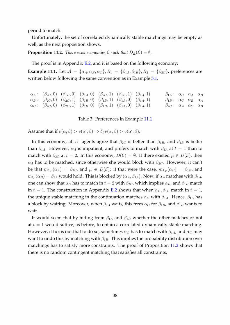
period to match.Unfortunately, the set of correlated dynamically stable matchings may be empty as

well, as the next proposition shows.

Proposition 11.2. There exist economies E such that D∆(E) = ∅.

The proof is in Appendix E.2, and it is based on the following economy:

Example 11.1. Let A = {αA, αB, αC}, B1 = {β1A, β1B}, B2 = {β2C}, preferences arewri en below following the same convention as in Example 5.1.

αA : (β2C , 0) (β1B, 0) (β1A, 0) (β2C , 1) (β1B, 1) (β1A, 1)αB : (β2C , 0) (β2C , 1) (β1B, 0) (β1B, 1) (β1A, 0) (β1A, 1)αC : (β2C , 0) (β2C , 1) (β1B, 0) (β1B, 1) (β1A, 0) (β1A, 1)

β1A : αC αA αB

β1B : αC αB αA

β2C : αA αC αB

Table 3: Preferences in Example 11.1

Assume that if v(α, β) > v(α′, β)⇒ δβv(α, β) > v(α′, β).

In this economy, all α−agents agree that β2C is be er than β1B, and β1B is be erthan β1A. However, αA is impatient, and prefers to match with β1A at t = 1 than tomatch with β2C at t = 2. In this economy, D(E) = ∅. If there existed µ ∈ D(E), thenαA has to be matched, since otherwise she would block with β2C . However, it can’tbe that m2,µ(αA) = β2C , and µ ∈ D(E): if that were the case, m1,µ(αC) = β1B, andm1µ(αB) = β1A would hold. This is blocked by (αA, β1A). Now, if αA matches with β1A,one can show that αC has to match in t = 2 with β2C , which implies αB, and β1B matchin t = 1. The construction in Appendix E.2 shows that when αB, β1B match in t = 1,the unique stable matching in the continuation matches αC with β1A. Hence, β1A hasa block by waiting. Moreover, when β1A waits, this frees αC for β1B, and β1B wants towait.

It would seem that by hiding from β1A and β1B whether the other matches or notat t = 1 would suffice, as before, to obtain a correlated dynamically stable matching.However, it turns out that to do so, sometimes αC has to match with β1A, and αC maywant to undo this by matching with β1B. This implies the probability distribution overmatchings has to satisfy more constraints. The proof of Proposition 11.2 shows thatthere is no random contingent matching that satisfies all constraints.

38

₁₂ D R L

12.1 Discussion

Implementation. Any dynamically stable matching can be sustained as the subgameperfect Nash equilibrium of a two-stage game based on the one introduced by Kalai[23]. In the second stage, agents a ∈ A who have not matched in the first stage, andthe remaining agents and new entrants on side B simultaneously announce an agentfrom the other side -or themselves-, coinciding announcements turn into matchings.In the first stage, fixed a realization of the arrivals, B1, agents in A ∪ B1 play the samegame as in stage two, but amongst themselves. When arrivals are deterministic, thecoalition-proof Nash equilibria of a second game, in which agents in A ∪ B1 ∪ B2 an-nounce simultaneously agents on the other side coincides with the core (see Kalai [23],Alcalde [4], Kara and Sönmez [24]). The different timings and equilibrium conceptscapture the assumptions embodied in the core, and dynamically stable matchings interms of the agreements agents can form between themselves. These implementationresults are presented in the Supplementary Material, Section S.1 .La ice When arrivals are stochastic, the “many-to-many” structure of the core (Sec-

tion 4.2) implies it no longer has the la ice property. This is in contrast with the caseof deterministic arrivals. These and other properties which are lost due to the “many-to-many” structure of the core in the case of stochastic arrivals are explored in depthin Doval [15]. However, even when arrivals are deterministic, the set of dynamicallystable matchings does not have the la ice structure (see Appendix S.2).Different intertemporal orders derived from ▷b: I only consider objects which are,

in a sense, extremely patient: between matching in t = 1 with a, and matching at some(2, B2) with a′ ▷a, the second matching is chosen. A different definition is one in whichthe objects’ ranking is used to decide between different t = 1 matching partners, ordifferent matching partners at (2, B2) for some B2, but matching in t = 1 is prioritizedover matching in t = 2. What the correct assumption is depends on the se ing. Thefirst assumption may be suitable in cases in which one is concerned with market thick-ness, so that saving the objects to match later is useful - see for instance Akbarpouret al. [3]. The second assumption is be er suited in se ings in which matching rightaway, instead of who matches with whom is more relevant. Note that if the objectsprioritize matching in t = 1, it is as if they discount the future. Hence, the conditionsfor existence will resemble more those of the two-sided market.Non-storable objects The assumption that objects are storable plays no role in Sec-

tion 5.2; all results would go through if objects are non-storable. This is good since the

39

allocation of deceased-donor organs falls in the non-storable objects case. However,the result, in Section 5.1, that core matchings fail to be dynamically stable follows frommatching opportunities not expiring.23 Given the applications considered in those sec-tions (adoption markets, job markets, public housing), the assumption is reasonable.But, there is an interesting extension to consider in light of Remark 10.2. In the exam-ple presented there, b prefers to match with a less preferred agent a2 over matching int = 2 with a more preferred agent, a1, only when a1’s most preferred matching part-ner, b∗, does not arrive. I interpret this as b tending a1 an exploding offer to match int = 1.24 Matching with contracts allows one to model this explicitly: a1 and b can signone of two contracts, one in which they either match in t = 1, and which expires int = 1 (i.e. the exploding offer), and one in which a gets to pick when to match with b

(i.e. an option contract). Of course, the existence of the first contract implies that b canpromise not to match in t = 2 with a1, if they both remain unmatched. By allowing forcontracts with different terms and expiration dates, matching with contracts allows fora richer set of binding agreements in this se ing. However, suppose there is a thirdcontract between a1 and b, which b can offer to a1 in t = 2. Even if the exploding offeris an option, the question still remains of whether or not, in t = 2, b, after a1 rejects theexploding offer, will offer this contract to a1. a1’s decision to reject the exploding offerdepends on her expectations about b’s offer in t = 2. Thus, even in the richer se ing,all the issues raised in this paper are still relevant. Studying this extension in depth isleft for future research.

12.2 Related Literature

The paper relates to several strands of literature. I focus here on the relation with theliterature on dynamic matching markets; other related papers have been referencedthroughout the main text. To the best of my knowledge, Kurino [29] is the first tointroduce into a dynamic matching problem the notion that a matching should be acomplete contingent plan; he analyzes a repeated matching market in which men andwomen match every period, and does not ask for credible continuations (see Example1 in the paper).25 In independent and contemporaneous work, Kadam and Kotowski[22] analyze a two-period repeated matching market as in Kurino [29], introducing astability notion which they also denote dynamic stability, but applies to on-path match-

23Proposition S.4 in the Supplementary Material shows that when the core is non-empty, and match-ing opportunities expire, then the set of dynamically stable matchings is non-empty.

24Recall that b’s reticence to wait “forces” a1 to match with him instead of obtaining her most pre-ferred outcome.

25Damiano and Lam [13], and Bando [8] analyze similar se ings

40

ings.26 Pais [33], and Niederle and Yariv [32] study conditions under which a decentral-ized two-sided market sustains static stable outcomes. Kurino [30], Kennes [26] andPereyra [34] provide stability notions for allocating objects to overlapping generationsof agents, where the main concern is to respect the property rights over the objects in-duced by the allocation in the previous periods. In a similar vein, Compte and Jehiel[12] analyze a two period model where matching happens in the last period, but theexogenously given allocation in the first period determines the outside option in thesecond period. Ünver [48] considers the problem of kidney exchange where agents andtheir paired donors arrive to an exchange pool over time, and characterizes the optimalmechanism for two-way and multi-way exchanges. Leshno [31] considers the problemof allocating objects which arrive over time to a group of agents, who arrive over time,with unobservable preferences for the objects, and assumes objects have to be assignedupon arrival. Akbarpour et al. [3] consider a networked market where agents are indif-ferent between their feasible matches, but the planner may want the agents to wait tobe matched to facilitate others’ matchings. Schummer [45] analyzes the issues with in-fluencing waiting lists when agents are served on a first-come-first-serve basis. Thakral[47] considers algorithms for allocating objects with and without priorities, which ar-rive stochastically over time and have to be allocated upon arrival. None of the existingpapers touch upon the issues that are relevant in the present work, namely, the inter-action between the value of waiting for a be er match, and the assumptions on thebinding agreements agents can form, and how this relates to the appropriate notion ofstability in each se ing.

Some of the ideas presented in the paper have appeared in more recent work. Bac-cara et al. [6] consider a two-sided market in which agents face a trade-off betweenmatching immediately with a low type and waiting for a high type agent of the op-posite side. Kotowski [28] incorporates the idea of contingent stability to a repeatedmatching market.

₁₃ C

Dynamic matching markets such as adoption markets, the allocation of public hous-ing, and of deceased-donor organs share three key features: (i) matching opportunitiesarrive over time, (ii) matching is one-to-one, and (iii) matching is irreversible. In thesemarkets, agents face a dynamic decision problem: an agent can match today, thus, ex-iting the pool of the unmatched agents, or she may remain unmatched this period, andkeep the option of matching with a (potentially be er) matching partner tomorrow.

26See Remark 4.1

41

Despite their similarities, the three markets mentioned above deal differently withthe option of waiting for a be er match: some adoption agencies limit adoptive par-ents’ option to wait to be matched, the PHA dismisses agents from the waiting list afterrejecting compatible housing offers, and UNOS does not penalize patients who refusethe offer to receive a transplant. The framework developed in this paper rationalizesthe rules implemented by the different clearinghouses.

In order to understand why markets that look (a priori) similar have in place so dif-ferent rules, the present paper proceeds in three steps. First, because matching marketswith properties (i)-(iii) above have not been studied in the literature, I define a naturalstability notion for these markets. I denote it dynamic stability. Second, I show that fortwo-sided economies (and, hence, for the allocation of objects with priorities) dynam-ically stable matchings may fail to exist. This non-existence problem arises preciselybecause agents have the option to wait for be er matching opportunities. Adoptionmarkets and the allocation of public housing correspond, respectively, to two-sidedeconomies, and the allocation of objects with priorities. In contrast, in markets suchas the allocation of deceased-donor organs dynamically stable matchings always exist.It follows from these two observations that in the first two markets a central clearinghouse which regulates agents actions, in particular, what happens after they reject acurrent offer in order to wait for a be er match, is needed to guarantee the allocationis efficient. Third, in markets such as adoption markets, and public housing, I providesufficient conditions under which dynamically stable matchings exist. Hence, underthese conditions, the clearing house need not restrict agents’ actions in order to guar-antee efficiency.

A P S ₅.₁

A.1 Proof of Proposition 5.1

I start by specifying the matchings at the different continuation histories; the terms in the curlybrackets indicate who matched in t = 1 (if any):

Step 1: There is no dynamically stable matching µ in which αC is unmatched. Hence, in anyµ ∈ D she matches with β1B , or β2C . This is because if αC is unmatched, she blocks withβ2C .

Step 2: There is no µ ∈ D such that αC matches with β2C . Said contingent matching wouldhave to match αB with β1B , and αA with β1A. However, αB blocks by waiting to bematched with β2C since that is her outcome in the unique continuation when αA, β1Amatch in t = 1.

Step 3: There is no dynamically stable matching in which αC matches with β1B . Said contin-gent matching would have to match αB with β2C - otherwise (αB, β1B) block-, and αA

42

(αA, β1A) at t = 1

αB β1B

αC β2C

∅ β2D

(αB, β1B) at t = 1

αA β1A

αC β2C

∅ β2D

(αC , β1B) at t = 1

αA β2C

αB β2D

∅ β1A

∅ at t = 1

∅ β1A

αA β1B

αB β2C

αC β2D

with β1A. However, this is blocked by αA waiting to be matched in t = 2 since whenαC , β1B matches in t = 1, αA gets matched with β2C in t = 2.

Steps 1-3 imply that D(E) = ∅.

A.2 Remark 10.2: Non-existence with stochastic arrivals

Example A.1. There exist economies E with stochastic arrivals such that D(E) = ∅.

Proof. Let A = {α1, α2}, B = {b1, b2}, and supp G = {(b1, b2), (b1, ∅)} = {B2, B2}, where

r1 = G(B2). Preferences are given by:

(∀b ∈ B)v(α2, b) > v(α1, b)

(∀α ∈ A)u(α, b2) > u(α, b1)

v(α2, b1) > v(α1, b1) > δb1 [r1v(α2, b1) + (1− r1)v(α1, b1)]

u(α1, b1) > δα1 [r1u(α1, b1) + (1− r1)u(α1, b2)]

δα2 [r1u(α2, b1) + (1− r1)u(α2, b2)] > u(α2, b1) > δα2(1− r1)u(α2, b2)

Both β−agents agree that α2 is the best, while both α−agents agree that b2 is the best. How-ever, there is uncertainty about b2’s arrival. α1 prefers to match immediately with b1 to wait andmatch with the best available β−agent. α2 holds exactly the opposite preferences. Moreover,α2 is willing to match with b1 if the alternative is to match only with b2 if he arrives. Finally, b1prefers to match with α1 to match contingently with α1 on B

2 and with α2 on B2.Note that if both α1 and α2 are present in t = 1, any stable match assigns the best available

β−agent to α2, and the remaining (if any) to α1, and if only one α−agent remains she getsthe best remaining β−agent (if any). Moreover, note that any dynamically stable contingentmatching has to satisfy that: (i) no β−agent remains unmatched, and (ii) b1 is matched at t = 1.

Given the above, consider the contingent matchingµ that has the on-path matching: m1(B1)(α1) =

b1,m1(B1)(α2) = α2,m2(B2)(α2) = α2,m2(B

2)(α2) = b2, and specifies µ(h2) taking into ac-

count the above. However, µ is blocked at t = 1 by (α2, b1), since α2 prefers to match with b1,and b1 gets his most preferred α−agent.

43

The only other possible contingent matching isµ′ that has the on-path matching: m′1(B1)(α1) =

α1,m′1(B1)(α2) = b1,m

′2(B

2)(α1) = α1,m′2(B

2)(α1) = b2. However, since µ′(h2)(α2) = b2 for

h2 = (B1, m1, B2), m1(k) = k, and µ′(h2)(α2) = b1 for h2 = (B1, m1, ∅), m1(k) = k, α2 blocksby waiting to be matched at t = 2.

B P S ₅.₂

B.1 Proof of Proposition 5.2 for economies with deterministic arrivals

The proof follows from the following definition, and two lemmas.Let g : {1, ..., |A|} 7→ A be an ordering of the α−agents. Consider the matching mg ∈ M

such that g(1) gets her most preferred element in B1∪B2, b∗(g(1)); g(2) gets her most preferredelement in B1∪B2\{b∗(g(1))}; g(l) gets her most preferred element in B1∪B1\

∪l−1i=1{b∗(g(i))};

where most preferred is defined using the preferences at the initial period. For each h2 ∈ H2,let mg

2(h2) be the allocation for the submarket ⟨A(h2),B(h2)⟩ obtained by the same procedure

as before using ordering g(B1) = g|A(h2) and le ing α−agents pick objects in B(h2).Definition B.1. The sequential dictatorship contingent matching when agents are ordered ac-cording to g, µg, is the element ofM, such thatmµg = mg; and for allh2 ∈ H2, µ(h2)|A(h2)∪B(h2) =mg

2(h2).

Lemma B.1. Fix an economy E with deterministic arrivals; and fix g : {1, ..., |A|} 7→ A aninjective function. Then, µg defined in Definition B.1 is dynamically Pareto efficient.

Proof. By construction, it is only necessary to show that there are no blocks at t = 1.

Step 1: If (A′, µ′) is a block of µg at t = 1 then there exists a ∈ A′ such that µ′(B1)(a) = a.

Proof. By contradiction. Suppose not. Then,

(∀a ∈ A′)µ′(B1)(a) ∈ ∪a′∈A′{µg(B1)(a′)} ∪ {b ∈ B1 : (∀a ∈ A)b = µg(B1)(a)}

Moreover, since (∀l ≥ 0){b ∈ B1 : (∀a ∈ A)b = µg(B1)(a)} ⊂ B1 ∪B2\ ∪lk=1 {b∗(g(k))} (where,for l = 0, ∪lk=1{b∗(g(k))} = ∅) the unassigned buildings at t = 1 are available to α−agentg(l + 1) for all l ≥ 0, and it cannot be the case that ∃a ∈ A′ : µ′(B1)(a) ∈ {b ∈ B1 : (∀a ∈ A)b =µg(B1)(a)}.

Thus, (∀a ∈ A′)µ′(B1)(a) ∈ ∪a′∈A′{µg(B1)(a′)}. Let a = arg min{g−1(a) : a ∈ A′}. Note that:

µ′(B1)(a) ∈∪

a′∈A′

{µg(B1)(a′)} ⊆ B1 ∪B1\

g−1(a)−1∪k=1

{b∗(g(k))}

Hence, µ′(B1)(a) was available for a to choose when it was her turn under g, which contradictsthat u(a, µ′(B1)(a)) > U(a,mg, B1).

Step 2: There are no blocks (A′, µ′) at t = 1 such that (∃a ∈ A′) : µ′(B1)(a) = a.

Proof. By contradiction. Let (A′, µ′) be a block of µg at B1. By step 1, it follows that there existsa ∈ A′ : µ′(B1)(a) = a. Moreover, le ing a = arg min{g−1(a) : a ∈ A′}, the proof of Step 1shows that µ′(B1)(a) = a.

Let h2mµ′be the continuation history induced by the block, i.e. h2mµ′

= (B1,m1,µ′ , B2), and let

44

m2,µ′ = µ(h2mµ′)|A(h2

mµ′)∪B(h2

mµ′ ).

Let b∗ = m2,µ′(a). Note that (i) b∗ ∈∪g−1(a)−1

k=1 {b∗(g(k))}, and (ii) b∗ ∈ B2. The first followsfrom the fact that otherwise b∗ would have been available for a to choose. The second followsfrom the fact that b∗ can’t have been assigned in t = 1 to another α−agent, b∗ can’t have beenassigned at t = 1 to a ∈ A′\{a} by definition of a, and Step 1, and, finally, b∗ can’t be anunassigned building available at t = 1 which would contradict (i).

Hence, there exists a∗ ∈ A : mg(a∗) = b∗, and g−1(a∗) < g−1(a).Define a0 = arg min{g−1(a) : a ∈ A(h2mµ′

)}. Note that g−1(a0) ≤ g−1(a∗) < g−1(a). Note thatb∗(a0) continues to be a0’s choice at h2mµ′

. This follows from the fact that the set of buildingsavailable at h2mµ′

, B(h2mµ′) is such that:

B(h2mµ′) ∩B1 = {b ∈ B1 : µ

′(B1)(b) = b}

= {b ∈ B1 : µ(B1)(b) = b} ∪ {b ∈ B1 : µ(B1)(b) ∈ A′ ∧ µ′(B1)(b) = b}

Hence, all the buildings available because of the block were available for a0 to choose fromwhen it was her turn under g. Therefore, she chooses b∗(a0) again.

Inductively, (∀a ∈ A(h2mµ′)) : g−1(a) ∈ {g−1(a0) + 1, ..., g−1(f∗)}, b∗(a) continues to be their

most preferred choice out of B(h2mµ′)\∪g−1(a)−1

k=1 {b∗(g(k))}. In particular, a∗ chooses b∗. Thiscontradicts that a obtains b∗ at h2mµ′

, and hence, that there is a block at B1.

LemmaB.2. Fix an economy with deterministic arrivals. Letm ∈M be a Pareto efficient match-ing. Then, there exists g : {1, ..., |A|} 7→ A such that mg = m.

Proof. Step 1: In any Pareto efficient allocation m∗ ∈ M , there exists a ∈ A such that m∗(a) ∈arg maxm∈M U(a,m).

Proof. Suppose not. Then, (∀a ∈ A) m∗(a) /∈ arg maxm∈M U(a,m). Consider the followinggraph. Nodes are given by A ∪ B1 ∪ B2. Edges are as follows: each a ∈ A points to her mostfavorite element in {a} ∪ B1 ∪ B2. Each b ∈ B1 ∪ B2 points to the α−agent to which it wasallocated under m∗ (or to itself otherwise).

Note that since (∀a ∈ A)m∗(a) /∈ arg maxm∈M U(a,m), no a ∈ A points to m∗(a). Moreover,since m∗ is Pareto efficient, no a ∈ A points to an unassigned building.

Claim: If ∃a ∈ A : m∗(a) = (a, a) then there exists a cycle. Fix a0 ∈ A, and follow the directedpath starting at a0, p = (a0b0a1b1...anbn). Note that each bl ∈ p is such that bl = m∗(al+1), andnote that al+1 never points to bl. Since the graph is finite, the path stops at some point. I claim itforms a cycle. Say the path ends at an unreached b ∈ B1 ∪B2, such that m∗(b) = a. Then, b hasto point to a, a contradiction to the path ending (note that the discussion before implies thatthe path cannot end at a b : m∗(b) = b). Say that the path ends at an unreached a ∈ A. But thena points to his most favorite available building. Hence, there is a cycle. Moreover, each agentis be er off with the building his pointing at than with his own. Hence, we obtain a Paretoimprovement by having the agents in the cycle exchange their own buildings, a contradictionto m∗ being Pareto efficient.

45

Applying inductively the proof of Step 1, Step 2 below follows. Define:

A1 = {a ∈ A : m∗(a) ∈ arg maxm∈M

U(a,m,B1)}

M1 = {m′ ∈M : (∀a ∈ A1)m′(a) = m∗(a)}

An =n−1∪i=1

Ai ∪ {a ∈ A : m∗(a) ∈ arg maxm∈Mn−1

U(a,m,B1)}

Mn = {m′ ∈M : (∀a ∈ An)m′(a) = m∗(a)}

Step 2: (∀n ≥ 1)(∃a ∈ A\An) : m∗(a) ∈ arg maxm∈Mn U(a,m,B1).

Step 3: Define g : {1, ..., |A} 7→ A to be such that (∀n < n′)(∀a ∈ An)(∀a′ ∈ An′)g−1(a) <

g−1(a′). Then, mg = m∗.

Proof. This follows from revealed preference, and the definitions in Steps 1 and 2.

B.2 Proof of Proposition 5.2 for economies with stochastic arrivals

The proof of Proposition 5.2 for economies with stochastic arrivals has two parts. First, I showthat the analog of µg for economies with stochastic arrivals is dynamically Pareto efficient.Then, I show that not all Pareto efficient allocations can be achieved by a serial dictatorship,and, after defining a different contingent matching based on the YRMH-IGYT mechanism ofAbdulkadiroğlu and Sönmez [1], I show that the contingent matchings generated in that wayare dynamically Pareto efficient.

B.2.1 Serial Dictatorship

Let g : {1, ..., |A|} 7→ A be an ordering of the α−agents. Considering the allocation mg ∈ Mconstructed as follows. Firm g(1) chooses: m∗

g(1) ∈ arg maxm∈M U(g(1),m). Define M(g(1)) =

{m′ ∈ M : m′(g(1)) = m∗g(1)(g(1))}. Inductively, define M(g(1)...g(n)) = {m′ ∈ M : (∀i ∈

{1, ..., n})m′(g(i)) = m∗g(i)(g(i))}, and let

m∗g(n+1) ∈ arg maxm∈M(g(1),...,g(n)) U(g(n + 1),m). Let mg ∈ M be the allocation constructed

in that way. For each h2, let mg(h2)|A(h2),B(h2) be the allocation obtained by serial dictatorshipusing g|A(h2). Let µg ∈ M be the contingent matching such that mµg = mg, and for all h2,µ(h2)|A(h2) = mg(h2)|A(h2).27 The proof of Lemma B.3 follows from the same steps as the proofof Lemma B.1 (though with slightly more notation) so it is stated without proof:Lemma B.3. Fix an economy E . Then, µg is dynamically Pareto efficient.

B.2.2 YRMH-IGYT mechanism

Example B.1 (Not all Pareto efficient allocations can be obtained by serial dictatorship). Con-sider the following economy based on the one in Proposition A.1. There are two α−agents

27Recall that, by definition of a contingent matching, the matching at h2 specifies that the α−agentsand buildings that were matched at t = 1 continue to be matched together

46

A = {a1, a2}, and arrivals are as follows: B2 = {b1, ∅}, B2= {b1, b2}. Let r1 = Pr(B2). Prefer-

ences are given as follows:

u(ai, b2) > u(ai, b1), i = 1, 2

δa2 [r1u(a2, b1) + (1− r1)u(a2, b2)] > u(a2, b1) > δa2(1− r1)u(a2, b2)

u(a1, b1) > δa1 [r1u(a1, b1) + (1− r1)u(a1, b2)]

The following matching is Pareto efficient: m1(B1)(a1) = a1,m2(B2)(a1) = a1,

m2(B2)(a1) = b2,m1(B1)(a2) = m2(B

2)(a2) = m2(B2)(a2) = b1. Pareto efficiency follows

from: (i) any allocation that makes a2 be er off has to match her with b2 at B2, and with b1 atB2, which implies a1 can only match with b1 at B2, and u(a1, b1) < u(a1, b2), and (ii) any alloca-tion that makes a1 be er off implies that the highest payoff a2 can obtain is δa2(1− r1)u(a2, b2).

However, this allocation cannot be obtained by a serial dictatorship: any allocation thatmakes a1 the dictator, matches a1 with b1 at t = 1, and any allocation that makes a2 the dictatormatches a2 as in (i) above. Still, as the next lemma shows, there is away of constructing thecontingent matching that implements any Pareto efficient allocation.Lemma B.4. Let m ∈ M be a Pareto efficient matching. Then, there exists µ ∈ M such thatmµ = m, and µ is dynamically Pareto efficient.

Proof. Fix m a Pareto efficient matching. Fix an order g : A 7→ {1, ..., |A|}. Let µ ∈ M be asfollows:

1. mµ = m. For each initial history, B1, and for each arrival history B2 = (B1, B2), and foreach h2 ∈ H2(B1), Let B2(h2) be the projection of h2 onto {(B1, B2) : (B1, B2) ∈ (2B)2}.

2. For all h2 ∈ H2(B1), let E(h2) = {a ∈ A(h2) : m2(B2(h2)) ∈ B(h2)}, and let BO(h2) =

m2(B2(h2))(E(h2)). E(h2) are the existing tenants, BO(h2) are the owned buildings,

A(h2)\E(h2) are the new tenants, and B(h2)\BO(h2) are the vacant houses. Let µ(h2) bethe allocation obtained from YRMH-IGYT algorithm applied to ⟨E(h2),A(h2),BO(h2),B(h2)\BO(h2)⟩using the order g|A(h2). (Note that potentially E(h2) may be empty, so that µ(h2) is a se-rial dictatorship).

Remark B.1. The following hold: (i) µ(h2) is Pareto efficient for all h2, and (ii) Let h2 be suchthat E(h2) = ∅, then all a ∈ E(h2) obtain at least u(a,m2(B

2(h2))(a)).

The remark implies that only blocks at B1 need to be ruled out. Towards a contradiction,fix B1, and let ⟨A′, µ′⟩, µ′ ∈ M(B1) be a block of µ at B1. Let H2

A′(B1) = {h2 ∈ H2(B1) :h2 = (B1, µ

′(B1), B2), B2 ⊆ B}, and let mµ′ be the on-path matching for µ′ at B1. Note that(∀a ∈ A\A′) : m1(B1)(a) = a, U(a,mµ;B1) = U(a,mµ′ , B1). Moreover, (∀a ∈ A\A′) :m1(B1)(a) = a, (∀h2 ∈ HA′(B1))m2(B

2(h2))(a) ∈ B(h2), whenever m2(B2(h2))(a) = a. There-

fore, for all such a, U(a,mµ′ , B1) ≥ U(a,mµ;B1), since a owns her original assignment at h2under the YRMH-IGYT mechanism. Finally, by definition of a block (∀a ∈ A′)U(a,mµ′ , B1) >U(a,mµ;B1). This contradicts m being Pareto efficient. Hence, there are no blocks at B1.

C P S ₆.₂

C.1 Proof of Proposition 6.3

Some lemmas are needed for the proof.

47

LemmaC.1. Letµ∗ ∈ C∗(E)Then, µ is dynamically stable if, and only if, there is no ⟨A′, B′, µ′⟩, A′∪B′ ⊂ A ∪B1 such that (∀k ∈ A′ ∪B′)m1,µ′(B1)(k) = k and ⟨A′, B′, µ′⟩ is a block of µ∗ at B1.

Lemma C.1 follows immediately from Definition 4.10.Definition C.1 (Objection to early matching). Given µ ∈M, a block of µ at B1 ⟨A′, B′, µ′⟩ suchthat (∀k ∈ A′ ∪B′)m1,µ′(B1)(k) = k is referred to as an objection to early matching.Lemma C.2. Fix an economy with deterministic arrivals, E , and µ∗ ∈ C∗(E). Let ⟨A′, B′, µ′⟩ bea block of µ∗ at t = 1. Suppose that A′, B′ = ∅. (∀b ∈ B1) if m1,µ∗(b) ∈ A′, then b /∈ B′.

Proof. Towards a contradiction, assume that (∃a ∈ A′) : m1,µ∗(a) ∈ B′. By Lemma C.1, (∀k ∈A′ ∪B′)m1,µ′(k) = k. Consider the t = 2−matching market originated by the block; i.e. le ingh2mµ∗

= (B1,m1,µ∗ , B2), h2mµ′ = (B1,m1,µ′ , B2), it follows that:

A(h2mµ′) = A(h2mµ∗ ) ∪m1,µ∗(B′) ∪A′,

B(h2mµ′) = B(h2mµ∗

) ∪m1,µ∗(A′) ∪B′

Let m2,µ′ = µ∗(h2mµ′). The proof follows from the following steps:

Step 1 (∀a ∈ A′)m2,µ′(a) ∈ m1,µ∗(A′) ∪B2, and m2,µ∗(m2,µ′(a)) = m2,µ′(a).

Proof. First, m2,µ′(a) ∈ m1,µ∗(A′) ∪B2. Suppose not, then m2,µ′(a) ∈ B′ ∪ {b ∈ B1 : m1,µ∗(b) =b}. This contradicts mµ∗ being an on-path matching for a core contingent matching. Clearly, ifm2,µ′(a) ∈ m1,µ∗(A′), then m2,µ∗(m2,µ′(a)) = m2,µ′(a). Hence, assume m2,µ′(a) ∈ B2. Then, ifm2,µ∗(m2,µ′(a)) = m2,µ′(a), (a,m2,µ′(a)) block µ∗ according to the core definition because m2,µ′

is individually rational, and v(a,m2,µ′(a)) > v(m2,µ′(a),m2,µ′(a)). Hence, m2,µ∗(m2,µ′(a)) =m2,µ′(a).

Now, ifm2,µ′(A′) = m1,µ∗(A′), the proof is done becauseµ∗ ∈ C(E) implies that (∀b ∈ m2,µ′(A′))v(m2,µ′(b), b) < v(m2,µ∗(b), b). However, this implies that (∀b ∈ m1,µ∗(A′))b /∈ B′. Hence, as-sume that m2,µ′(A′) = m1,µ∗(A′). Hence, by Step 1, (∃a ∈ A′) : m2,µ′(a) ∈ B2. Let n = |{a ∈A′ : m2,µ′(a) ∈ B2}|.

Moreover, note that (∀a ∈ A′) δau(a,m2,µ′(a)) > u(a,m1,µ∗(a)). Therefore, it has to be that(∀b ∈ m2,µ′(A′))v(m2,µ′(b), b) < v(m2,µ∗(b), b), otherwise µ∗ would not be in the core of E .

Step 2 LetAµ′≻µ∗(h2mµ∗

) = {a ∈ A(m2µ∗) : u(a,m2,µ′(a)) > u(a,m2,µ∗)(a)}, andBc,µ′≻µ∗

(h2mµ∗ ) =

{b ∈ B2 : m2,µ′(b) ∈ Aµ′≻µ∗(h2mµ∗

)}. Then,Aµ′≻µ∗(h2mµ∗ ) = ∅, andm2,µ∗(Bc,µ′≻µ∗

(h2mµ∗ )) ⊊Aµ′≻µ∗

(h2mµ∗).

Proof. To see thatAµ′≻µ∗(h2mµ∗

) = ∅, note that a ∈ A′ is such thatm2,µ′(a) ∈ B2, andm2,µ∗(m2,µ′(a)) ∈A. Let a = m2,µ∗(m2,µ′(a)). If u(a,m2,µ′(a)) < u(a,m2,µ∗(a)), then (a,m2,µ′(a)) block m2,µ′ , acontradiction. Hence, a ∈ Aµ′≻µ∗

(h2mµ∗).

Take b ∈ Bc,µ∗≻µ′(h2mµ∗

). Clearly, m2,µ∗(b) = b, since otherwise (b,m2,µ′(b)) block m2,µ∗ , acontradiction. Then, m2,µ∗(b) = b. If m2,µ∗(b) /∈ Aµ′≻µ∗

(h2mµ∗), then since m2,µ′(m2,µ∗(b)) = b,

it has to be that u(m2,µ∗(b), b) < u(m2,µ∗(b),m2,µ′(m2,µ∗(b))). If v(m2,µ∗(b), b) > v(m2,µ′(b), b),then (m2,µ∗(b), b) block m2,µ′ , a contradiction. Then,v(m2,µ∗(b), b) < v(m2,µ′(b), b), and hence (m2,µ′(b), b) block m2,µ∗ , a contradiction. Therefore,m2,µ∗(b) ∈ Aµ′≻µ∗

(h2mµ∗)

48

Step 2 implies that m2,µ∗(Bc,µ′≻µ∗) ⊂ Aµ′≻µ∗

(h2mµ∗). However, the inclusion is strict because

m2,µ∗(m2,µ′(a)) ∈ Aµ′≻µ∗(h2mµ∗ ), and m2,µ′(a) /∈ Bc,µ′≻µ∗ . Actually, it follows that |Bc,µ∗≻µ′ | ≤

|m2,µ∗(A′)| − n.

Step 3 m2,µ′(Aµ′≻µ∗(h2mµ∗

)) ∩ ({b ∈ B1 ∪B2 : m2,µ∗(b) = b} ∪B′) = ∅.

Proof. Towards a contradiction, suppose that (∃a ∈ Aµ′≻µ∗(h2mµ∗

)) : m2,µ∗(m2,µ′(a)) = m2,µ′(a).Since m2,µ′ is individually rational and a prefers her outcome under m2,µ′ to the one underm2,µ∗ , then (a,m2,µ′(a)) block µ∗ according to the core definition, a contradiction. Similarly, ifm2,µ′(a) ∈ B′, then (a,m2,µ′(a)) block µ∗, a contradiction. The result follows.

Note that |Bc,µ∗≻µ′(hm2

2,µ∗)| ≤ |{b ∈ B2 : m2,µ∗(b) ∈ Aµ′≻µ∗

(h2mµ∗ )}| − n = |Aµ′≻µ∗(h2mµ∗ )| − n,

and |{b ∈ B1 : m1,µ∗(b) ∈ A′ ∧ b /∈ B′ ∧ m2,µ′(b) /∈ A′}| ≤ n − 1, where the last inequalityfollows from assuming that there is at least one b ∈ m1,µ∗(A′) : b ∈ B′. This is a contradictionbecause by Step 3 the remaining β−agents can’t be matched to α−agents in Aµ′≻µ∗ , and (∀a ∈Aµ′≻µ∗

(h2mµ∗ ))m2,µ′(a) = a, and |m2,µ′(Aµ′≻µ∗(h2mµ∗

))| = |Aµ′≻µ∗(h2mµ∗ )|. Therefore, (∀b ∈

m1,µ∗(A′))b /∈ B′.Similarly, it follows that (∀a ∈ m1,µ∗(B′))a /∈ A′.

Lemma C.3. Fix an economy with deterministic arrivals E , and fix µ∗ ∈ C∗(E). Let ⟨A′, B′, µ′⟩be a block of µ∗ at t = 1. Let h2mµ′

= (B1,m1,µ′ , B2) denote the t = 2 history generated by theblock, and let m2,µ′ be the second period on-path matching for µ′, i.e. m2,µ′ = µ∗(h2mµ′

). Also,let h2mµ∗

= (B1,m1,µ∗ , B2) denote the on-path history for µ∗. Define:

Aµ′≻µ∗(h2mµ′ ) = {a ∈ A(h2mµ′ ) : δ

1[m2,µ′ (a)∈B2]a u(a,m2,µ′(a)) > δ

1[m2,µ∗ (a)∈B2]a u(a,m2,µ∗(a))}

Aµ∗≻µ′(h2mµ′

) = {a ∈ A(h2mµ′ ) : δ1[m2,µ′ (a)∈B2]a u(a,m2,µ′(a)) < δ

1[m2,µ∗ (a)∈B2]a u(a,m2,µ∗(a))}

Bµ′≻µ∗(h2mµ′

) = {b ∈ B(h2mµ′) : v(m2,µ′(b), b) > v(m2,µ∗(b), b)}

Bµ∗≻µ′(h2mµ′

) = {b ∈ B(h2mµ′) : v(m2,µ′(b), b) < v(m2,µ∗(b), b)}

The following hold:

Aµ′≻µ∗(h2mµ′

) ←→m2,µ′m2,µ∗ Bµ∗≻µ′

(h2mµ′)

Aµ∗≻µ′(h2mµ′

) ←→m2,µ′m2,µ∗ Bµ′≻µ∗

(h2mµ′)

{a ∈ A(h2mµ∗) : m2,µ∗(a) = a} = {a ∈ A(h2mµ′ ) : m2,µ′(a) = a}

{b ∈ B(h2mµ∗) : m2,µ∗(b) = b} = {b ∈ B(h2mµ′ ) : m2,µ′(b) = b}

Proof. Note that by definition:

Aµ′≻µ∗(h2mµ′

) = A′ ∪ Aµ′≻µ∗(h2mµ∗

),

Bµ′≻µ∗(h2mµ′

) = B′ ∪ Bµ′≻µ∗(h2mµ∗

)

It follows from Lemma A.3 that m2,µ′(Aµ′≻µ∗(h2mµ′

)) = m1,µ∗(A′) ∪ {b ∈ B2 : m2,µ∗(b) ∈Aµ′≻µ∗

(h2mµ∗ )} = m2,µ∗(A′ ∪ Aµ′≻µ∗(h2mµ∗

)) ⊆ Bµ∗≻µ′(h2mµ′

). Also, it follows from LemmaA.3 that m2,µ′(Bµ′≻µ∗

(h2mµ′)) = m1,µ∗(B′) ∪ {a ∈ A(h2mµ∗ ) : m2,µ∗(a) ∈ Bµ′≻µ∗

(h2mµ∗)} =

49

m2,µ∗(B′ ∪ Bµ′≻µ∗(h2mµ∗

)) ⊆ Aµ∗≻µ′(h2mµ′

).It remains to show that the weak inclusions are, in fact, equalities. This will also prove the

last two statements in the proposition. Suppose that m2,µ∗(A′∪Aµ′≻µ∗(h2mµ∗

)) ⊊ Bµ∗≻µ′(h2mµ′ ),

and let b ∈ Bµ∗≻µ′(h2mµ′ )\m2,µ∗(A′ ∪ Aµ′≻µ∗

(h2mµ∗)). Note that m2,µ′(b) = b. If m2,µ∗(b) = b,

then we have a contradiction. Then, assume that m2,µ∗(b) = b. Then, it has to be that m2,µ∗(b) ∈Aµ∗≻µ′

(·), otherwise (b,m2,µ∗(b)) blockm2,µ′ . However, this contradicts thatm2,µ′(Aµ′≻µ∗(h2mµ′ )) =

m2,µ∗(A′∪Aµ′≻µ∗(h2mµ∗

)). Hence, m2,µ∗(Aµ′≻µ∗(h2mµ′

)) = m2,µ′(Aµ′≻µ∗(h2mµ′

)) = Bµ∗≻µ′(h2mµ′ ).

The other statements are shown by similar steps.

I now use the previous lemmas to prove Proposition 6.3:

Proof. Fix an economy with deterministic arrivals E , and fix µ∗ ∈ C∗(E). Suppose ⟨A′, B′, µ′⟩ isa block at B1. By Lemma C.1, it has to be that ⟨A′, B′, µ′⟩ is an objection to early matching. Letmµ′ be the on-path allocation for µ′, and let h2mµ′

be the t = 2 history generated by the block,and let h2mµ∗

be the t = 2 history that was on-path for µ∗. Let m2,µ′ = µ(h2mµ′).

Suppose that A′ = ∅. Then, by Lemma C.3,

Aµ′≻µ∗(h2mµ′

) ←→m2,µ′m2,µ∗ {b ∈ B(h2mµ′

) : m2,µ∗(b) ∈ Aµ′≻µ∗(h2mµ′

)}

Construct the following graph. The nodes are Aµ′≻µ∗(h2mµ′ ) ∪ {b ∈ B(h2mµ′

) : m2,µ∗(b) ∈Aµ′≻µ∗

(h2mµ′ )}, and there is a directed edge from a to b if m2,µ′(a) = b, and there is a directededge from b to a if m2,µ∗(a) = b. Fix a ∈ A′, and follow the path starting from a. I claim thatthe path cycles. Since the graph is finite, the path stops at some node. Say that the node atwhich it stops is an unreached b: this is a contradiction since b ∈ {b ∈ B(h2mµ′

) : m2,µ∗(b) ∈Aµ′≻µ∗

(h2mµ′ )} implies that there is a directed edge from b to m2,µ∗(b) = b. Likewise, the pathcannot end at an unreached a ∈ Aµ′≻µ∗

(h2mµ′ ). Hence, the path cycles. Therefore, we have(a1b1a2b2...aNbN ) where28:

(∀i = 1...N)m2,µ′(ai) = bi

(∀i = 1, ..., N)m2,µ∗(ai+1) = bi

(∀i = 1, ..., N)δ1[bi∈B2]ai u(ai, bi) > δ

1[bi+1∈B2]ai u(ai, bi+1)

and, since µ∗ is in the core, it has to be that:

(∀i = 1, ..., N)v(ai+1, bi) > v(ai, bi)

Therefore, there is a simultaneous cycle. A similar result holds using Bµ′≻µ∗(h2mµ′

) when B′ =∅.

C.2 Proof of Proposition 6.4

Proof. Suppose towards a contradiction that (∃µ ∈ D(E)) : µ /∈ C∗(E). Then, there existsa ∈ A, and b ∈ B2 such that: δau(a, b) > u(a,m1µ(a)), and v(a, b) > v(m2µ(b), b). Now,since µ ∈ D(E), then a does not have a block by waiting. Hence, le ing µ′ ∈ M be such thatµ′(B1)(k) = µ(B1)(k), k /∈ {a,m1µ(a)}, µ′(B1)(k) = k otherwise, and (∀h2 ∈ H2(B1))µ

′(h2) =

28Indices are modulo N

50

µ(h2), it follows that δau(a,m2,µ′(a)) < u(a,m1µ(A)). Hence, v(m2,µ′(b), b) > v(a, b) by stabilityof m2µ′ at h2µ′ = (B1,m1µ′ , B2).

Let h2µ = (B1,m2µ, B2). Define B≻ = {b ∈ B(h2µ) : v(m2µ′(b), b) > v(m2µ(b), b)}, andF≻,c = {a ∈ A(h2µ) : m2µ′(a) ∈ B≻}.

Note B≻ = ∅ because b ∈ B≻. Moreover, |B≻\{b}| ≥ 1. Note first that if m2µ(m2µ′(b)) =m2µ′(b), then (m2µ′(b), b) block m2µ, a contradiction. Then, let b′ = m2µ(m2µ′(b)). Second, notethat if b′ /∈ B≻, then since m2µ′(b′) = m2µ(b

′), it has to be that v(m2µ′(b′), b′) < v(m2µ(b′), b′).

If m2µ′(b) prefers b to b′, then (m2µ′(b), b) block m2µ; otherwise, if m2µ′(b) prefers b′ to b, then(m2µ′(b), b′) block m2µ′ , both of which are contradictions. Hence, b′ ∈ B≻.

I claim that m2µ(A≻,c) ⊆ A≻. Take a ∈ Ac,≻. First, note that m2µ(a) = a, otherwise

(a,m2µ′(a)) block m2µ, a contradiction. Suppose then that b = m2µ(a) /∈ B≻. Then, by strictpreferences, and m2µ′(b) = a, it follows that v(m2µ′(b), b) < v(a, b). An argument similar to theone in the previous paragraph shows that this leads to a contradiction. Hence, b ∈ B≻, and theclaim follows.

Thus, m2µ′(B≻,c) ⊆ B≻, and m2µ(A≻,c) ⊆ B≻. Note that both m2µ′ ,m2µ are one-to-one and

map A≻,c into B≻. By Lemma 2.3 in Roth and Sotomayor [42], there exists ∅ = A ⊂ A≻,c suchthat m2µ(A) = m2µ′(A)(⊆ B≻).

I claim that |A| ≥ 2. Suppose not. Then, A = ∅ implies that |A| = 1, i.e. A = {a}. Thus,there exists b ∈ B≻ such that m2µ(b) = m2µ′(b), a contradiction to the definition of B≻. Hence,|A| ≥ 2.

Finally, consider a (directed) graph G = ⟨N , E⟩, with nodes N = A ∪ m2µ(A), and edges(a, b) ∈ E if b = m2µ(a), and (b, a) ∈ E if b = m2µ′(a). Pick a ∈ A, and follow the path start-ing from a. Since the graph is finite, the path stops. The definition of A implies that the patchcycles: it can’t stop at an unreached a or b. By the previous step, this implies there exists apreference cycle, a contradiction. Therefore, µ ∈ C∗(E).

D P S ₆.₃

D.1 Proof of Proposition 6.5

The proof follows from three steps. First, Proposition D.1 below states a property of cycleswhen priorities satisfy acyclicity. Second, fix µ ∈ C∗(E) such that mµ coincides with the match-ing obtained by side A proposing to agents on side B. The proof of Proposition 6.3 implies thatif there is a block by waiting, there has to be a cycle. The first step determines the cycle’s length.Third, the workings of deferred acceptance imply that the cycle is a two-cycle, a contradiction.DefinitionD.1. Let {▷b}b∈B be a priority structure for buildings. A sequence (a1, b1, ..., aN , bN ),N ≥ 2 is an improvement cycle if a1 ▷b1 a2... ▷bN aN .PropositionD.1. If {▷b∈B} satisfies Ergin-acyclicity, and (a1, b1, ..., aN , bN ) is an improvement cycle,then N = 2.

Proof. Let (a1, b1, ..., aN , bN ) be an improvement cycle, and suppose N > 2. Then, for all i ∈{1, ..., N − 1}ai ▷ ai+1, and aN ▷bN a1.

I claim that acyclicity implies (∀i)(∀j = i, i+ 1) aj ▷bi ai+1. First, note that acyclicity impliesthat (∀i)ai−1▷biai+1, where i = 1⇒ i−1 = N ; otherwise, ai▷biai+1▷biai−1▷bi−1

ai, violating Erginacyclicity. Hence, ai ▷bi ai+1, and ai−1 ▷bi ai+1. Similarly, it must be the case that ai−2 ▷bi ai+1;otherwise ai−1 ▷bi ai+1 ▷bi ai−2 ▷bi−2

ai−2 holds, violating acyclicity. Thus, ai ▷bi ai+1, ai−1 ▷bi ai+1,and ai−2 ▷bi ai+1, and we can proceed inductively and complete this for all j /∈ {i, i+ 1}.

51

Now, take j /∈ {i, i+1}. If aj ▷bi ai ▷bi ai+1 ▷bj−1aj - note that j− 1 = i. Then, it has to be that

ai ▷bi aj ▷bi ai+1 ▷bi−1ai, a contradiction.29 Thus, N = 2.

Now, consider µ ∈ C∗(E) such that mµ coincides with the outcome of deferred acceptancewith side A proposing to side B. Suppose µ /∈ D(E). Then, there exists A′ ⊆ A such that A′

blocks by waiting. It follows from the proof of Proposition 6.3 that ∃(b1, a1, ..., bN , aN ) suchthat δ1[bi+1∈B2]

ai u(ai, bi+1) > δ1[bi∈B2]ai u(ai, bi), and ai ▷bi ai+1. By Proposition D.1, it follows that

N = 2. Hence, write the cycle as (b1, a1, b2, a2). Moreover, from the proof of Proposition 6.3 itfollows that b1 = m2,µ(a1), b2 = m2,µ(a2).

Let r be the last step of the algorithm in which an agent in {a1, a2} makes an offer (and, isaccepted by) the building to whom she is matched under mµ. Without loss of generality, saythat a1 proposes to b1 at step r.

Let l ∈ {1, 2}. Since u(al,m2,µ(al+1)) > u(al,m2,µ(al)), al was rejected by m2,µ(al+1) beforestep r. Hence, at step r − 1, m2,µ(al+1) was matched to some agent, and at r − 1, b1 had anupstanding offer from some agent and it is not a2; otherwise a2 gets rejected in step r when a1makes an offer to b1. Hence, (∃a /∈ {a1, a2})such that a1 ▷b1 a ▷b1 a2. Since a2 ▷b2 a1, there is atwo-cycle, a contradiction. Therefore, µ ∈ D(E).

D.2 Proof of Proposition 10.5

Consider the following economy. A = {a1, a2}, B = {b1,1, b1,2, b2,1, b2,1}. Objects’ rankings are:

a1 ▷b1,1 a2

a2 ▷b1,2 a1

a2 ▷b2,1 a1

a1 ▷b2,1 a2

Arrivals are as follows. Let B1 = {b1,1, b1,2}, B2 = {b1,2}, B2 = {b2,1}. Then, G(B1, B2) = p,and G(B1, B2) = 1− p. Agents’ preferences are as follows:

δa1 [pu(a1, b1,2) + (1− p)u(a1, b1,2)] > u(a1, b1,1) > δa1 [pu(a1, b1,1) + (1− p)u(a1, b1,2)]

δa2 [pu(a2, b1,2) + (1− p)u(a2, b1,1)] > u(a2, b1,1) > u(a2, b1,2) > δa2 [pu(a2, b1,1) + (1− p)u(a2, b1,2)]

All objects that do not appear in the above rankings are deemed unacceptable. There is onlyone matching in the core: m1,µ(B1)(a2) = b1,1, m2,µ(B1, B2)(a1) = b2,1,m2,µ(B1, B2) = b2,1.That this is the unique matching in the core follows from two observations. First, there is nomatching in the core which both agents match in period 1. If a1 matches with b1,1 in t = 1, thena2 matches with b1,2 in t = 1 as well. Hence, a1 can block with b2,1, b2,1. Second, there is nomatching in which a2 matches in period 2. In this case, she would match with b1,1 at (B1, B2),but this is blocked by a1, b1,1.

Note, however, that the unique (on-path) matching in the core cannot be part of a dynamicallystable contingent matching: a2 can block by waiting and get her most preferred matching.

29Here is where N > 2 ma ers most, worst case scenario j = i− 1

52

E P S ₁₁

E.1 Proof of Proposition 11.1

From the proof of Proposition 5.1, it follows that for eachh2 ∈ H2 there is a unique stable match-ing. Let the random matching µ be as follows. With probability pq (the probabilities are definedbelow) (αB, β1B), (αA, β1A) are matched in t = 1, with probability q(1−p), (αC , β1B), (αA, β1A)are the ones to be matched in t = 1, with probability (1− q)p (αB, β1B) are the only ones to bematched in t = 1, and with probability (1− q)(1− p) (αC , β1B) are the only ones that match int = 1, that is µ puts positive probability on the following matchings (given the continuationsin the proof of Proposition 5.1):(

αA αB

β1A β1B

∥∥∥∥ αC ∅β2C β2D

)︸ ︷︷ ︸

pq

(αA αC

β1A β1B

∥∥∥∥ αB ∅β2C β2D

)︸ ︷︷ ︸

(1−p)q(αB

β1B

∥∥∥∥ αA αC ∅β1A β2D β2D

)︸ ︷︷ ︸

p(1−q)

(αC

β1B

∥∥∥∥ αA αB ∅β2C β2D β1A

)︸ ︷︷ ︸

(1−p)(1−q)

where:

p =δαAu(αA, β2C)− u(αA, β1A)

δαA(u(αA, β2C)− u(αA, β1A))

q =u(αB, β1B)− δαBu(αB, β2D)

δαB (u(αB, β2C)− u(αB, β2D))

I show that the random contingent matching defined this way has no blocks. Recall that thedefinition of correlated dynamic stability requires that we consider only coalitions of size 2 and1.

Step 1: No α−agent or β−agent blocks by waiting to be matched.

1. When αB is informed that she is matched with β1B , if she decides to wait, she obtains:

qδαBu(αB, β2C) + (1− q)δαBu(αB, β2D) = u(αB, β1B)

where I used that αA conditions on her being matched with β1B , and the definition of q.

2. Whenβ1B is informed that he is matched withαB , sinceαB is his most preferredα−agent,there is no benefit in waiting to be matched.

3. When αA is informed she is matched with β1A, by waiting to be matched in t = 2, sheobtains:

pδαAu(αA, β1A) + (1− p)δαAu(αA, β2C) = u(αA, β1A)

where I used the definition of p. Hence, αA does not block by waiting to be matched int = 2.

4. Notice that β1A can never gain by matching later, hence there is no block involving β1A.

53

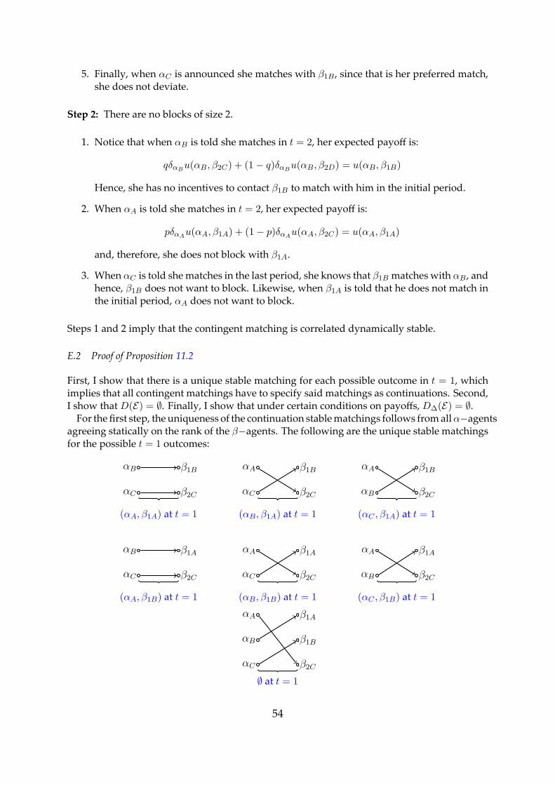
5. Finally, when αC is announced she matches with β1B , since that is her preferred match,she does not deviate.

Step 2: There are no blocks of size 2.

1. Notice that when αB is told she matches in t = 2, her expected payoff is:

qδαBu(αB, β2C) + (1− q)δαBu(αB, β2D) = u(αB, β1B)

Hence, she has no incentives to contact β1B to match with him in the initial period.

2. When αA is told she matches in t = 2, her expected payoff is:

pδαAu(αA, β1A) + (1− p)δαAu(αA, β2C) = u(αA, β1A)

and, therefore, she does not block with β1A.

3. When αC is told she matches in the last period, she knows that β1B matches with αB , andhence, β1B does not want to block. Likewise, when β1A is told that he does not match inthe initial period, αA does not want to block.

Steps 1 and 2 imply that the contingent matching is correlated dynamically stable.

E.2 Proof of Proposition 11.2

First, I show that there is a unique stable matching for each possible outcome in t = 1, whichimplies that all contingent matchings have to specify said matchings as continuations. Second,I show that D(E) = ∅. Finally, I show that under certain conditions on payoffs, D∆(E) = ∅.

For the first step, the uniqueness of the continuation stable matchings follows from allα−agentsagreeing statically on the rank of the β−agents. The following are the unique stable matchingsfor the possible t = 1 outcomes:

αB β1B

αC β2C

(αA, β1A) at t = 1

αA β1B

αC β2C

(αB, β1A) at t = 1

αA β1B

αB β2C

(αC , β1A) at t = 1

αB β1A

αC β2C

(αA, β1B) at t = 1

αA β1A

αC β2C

(αB, β1B) at t = 1

αA β1A

αB β2C

(αC , β1B) at t = 1

αA β1A

αB β1B

αC β2C

∅ at t = 1

54

For the second step, note the following: (i) Any dynamically stable contingent matching has tomatch two α−agents with two β−agents in t = 1, (ii) As argued in the main text, there is nodynamically stable contingent matching that matches (αA, β1A), (αB, β1B) in t = 1, since this isblocked by β1A, (iii) Any dynamically stable contingent matching that matches αC in the initialperiod, has to match αC with β1B , (iv) There is no dynamically stable contingent matching thatmatches (αC , β1B) and has αA wait to be matched with β2C since αA blocks it with β1A, (v)There is no dynamically stable contingent matching that matches αC with β1B , and αA withβ1A, since αC blocks by waiting to be matched with β2C . Hence, there is no dynamically stablecontingent matching.

For the third step, I prove the following lemma:Lemma E.1. Assume that the following holds:

δαC [Bu(αC , β2C) + (1−B)u(αC , β1B)] > u(αC , β1B)

u(αC , β1B) > δαC [Bu(αC , β1B) + (1−B)(Au(αC , β1A) + (1−A)u(αC , β1B))]

A =v(αA, β1A)− δβ1A

v(αB, β1A)

δβ1A(v(αC , β1A)− v(αB, β1A))

B =δβ1B

v(αC , β1B)− v(αB, β1B)

δβ1B(v(αC , β1B)− v(αB, β1B))

Then, D∆(E) = ∅.

Proof. Let µ be a random contingent matching.

Step 1: If m1 ∈ supp µ(B1), then m1(αC) = β1A.

Proof. Otherwise, (αC , β1B) block.

Step 2: If m1 ∈ supp µ(B1), then m1(αB) = β1A.

Proof. If m1 ∈ supp µ(B1) is such that m1(αB) = β1A, then it has to be that m1(αA) = β1B ,otherwise, (αA, β1A) block. However, this means that (αB, β1B) block.

Similarly, we have that:

Step 3: If m1 ∈ supp µ(B1), then m1(αA) = β1B .

Proof. If m1 ∈ suppµ(B1) and m1(αA) = β1B , then m1(αB) = αB , and there exists p > 0 suchthat:

U(αB, µ|E(m1(αB)), B1) = δαB [pu(αB, β2C) + (1− p)u(αB, β1A)] ≥ u(αB, β1B).

However, p > 0 implies that ∃m1 ∈ E(m1(αB)) such that m1(αC) = β1A - otherwise, αB cannotbe matched to β−agent β2C in t = 2 -, and by Step 1 this contradicts that µ ∈ D∆(E). Thus, ifm1 ∈ suppµ(B1), then m1(αA) = β1B .

55

Then, consider the following t = 1 matchings:

m1 : m11(αA) = β1A m1

1(αC) = β1B m11(αB) = αB

m2 : m21(αA) = αA m2

1(αC) = β1B m21(αB) = αB

m3 : m31(αA) = β1A m3

1(αC) = αC m31(αB) = β1B

m4 : m41(αA) = β1A m4

1(αC) = αC m41(αB) = αB

m5 : m51(αA) = αA m5

1(αC) = αC m51(αB) = β1B

m6 : m61(αA) = αA m6

1(αC) = αC m61(αB) = αB

Let pi = µ(B1)(mi1), i = 1, 2, ..., 6.

Step 4: If p1 + p2 > 0, then p1p1+p2

≤ (1−δαC)u(αC ,β1B)

δαC(u(αC ,β2C)−u(αC ,β1B)) ≡ D.

Proof. Conditional on being informed that she matches with β1B at t = 1, αC should not haveincentives to wait to be matched in t = 2, that is:

u(αC , β1B) ≥ δαC

[p1

p1 + p2u(αC , β2C) +

p2p1 + p2

u(αC , β1B)

].

The result follows immediately.

Corollary E.1. If p2 = 0, then p1 = 0.

Step 5: If p1 + p3 + p4 > 0, then p3p1+p3+p4

≤ v(αA,β1A)−δβ1Av(αB ,β1A)

δβ1A (v(αC ,β1A)−v(αC ,β1A)) ≡ A.

Proof. Conditional on being informed that he matches with αA at t = 1, β1A should not wantto wait to be matched in t = 2, that is:

v(αA, β1A) ≥ δβ1A

[p1 + p4

p1 + p3 + p4v(αB, β1A) +

p3p1 + p3 + p4

v(αC , β1A)

].

The result follows from the above equation.

Step 6: If p3 + p4 + p5 + p6 > 0, then:

u(αC , β1B) ≤

δαC

[p3+p4

p3+p4+p5+p6u(αC , β1B) +

p5p3+p4+p5+p6

u(αC , β1A)

+ p6p3+p4+p5+p6

u(αC , β1B)

]. (1)

Proof. Conditional on being informed that she does not match in t = 1, αC should not want toblock with β1B , that is equation (1) should hold.

Step 7: If p3 + p5 > 0, then p3p3+p5

≥ δβ1B v(αC ,β1B)−v(αB ,β1B)

δβ1B (v(αC ,β1B)−v(αB ,β1B)) .

Proof. Conditional on being informed that he matches in t = 1, β1B should not want to wait,that is:

v(αB, β1B) ≥ δβ1B

[p3

p3 + p5v(a3, b3) +

p5p5 + p3

v(αC , β1B)

]56

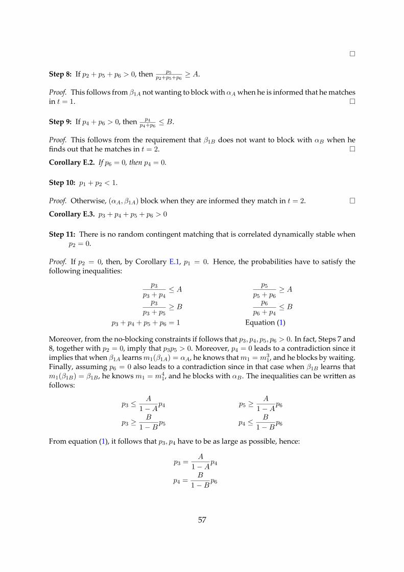
Step 8: If p2 + p5 + p6 > 0, then p5p2+p5+p6

≥ A.

Proof. This follows from β1A not wanting to block with αA when he is informed that he matchesin t = 1.

Step 9: If p4 + p6 > 0, then p4p4+p6

≤ B.

Proof. This follows from the requirement that β1B does not want to block with αB when hefinds out that he matches in t = 2.

Corollary E.2. If p6 = 0, then p4 = 0.

Step 10: p1 + p2 < 1.

Proof. Otherwise, (αA, β1A) block when they are informed they match in t = 2.

Corollary E.3. p3 + p4 + p5 + p6 > 0

Step 11: There is no random contingent matching that is correlated dynamically stable whenp2 = 0.

Proof. If p2 = 0, then, by Corollary E.1, p1 = 0. Hence, the probabilities have to satisfy thefollowing inequalities:

p3p3 + p4

≤ Ap5

p5 + p6≥ A

p3p3 + p5

≥ Bp6

p6 + p4≤ B

p3 + p4 + p5 + p6 = 1 Equation (1)

Moreover, from the no-blocking constraints if follows that p3, p4, p5, p6 > 0. In fact, Steps 7 and8, together with p2 = 0, imply that p3p5 > 0. Moreover, p4 = 0 leads to a contradiction since itimplies that when β1A learns m1(β1A) = αA, he knows that m1 = m3

1, and he blocks by waiting.Finally, assuming p6 = 0 also leads to a contradiction since in that case when β1B learns thatm1(β1B) = β1B , he knows m1 = m4

1, and he blocks with αB . The inequalities can be wri en asfollows:

p3 ≤A

1−Ap4 p5 ≥

A

1−Ap6

p3 ≥B

1−Bp5 p4 ≤

B

1−Bp6

From equation (1), it follows that p3, p4 have to be as large as possible, hence:

p3 =A

1−Ap4

p4 =B

1−Bp6

57

Moreover, it has to be the case that p5 > 0, otherwise the above inequalities imply that pi =0, i ∈ {3, 4, 5, 6}, a contradiction. Then, A

1−Ap6 ≤ p5 ≤ 1−BB p3 = A

1−Ap6. Hence, we obtain:p3 = AB, p4 = B(1− A), p5 = A(1− B), p6 = (1− A)(1− B). However, from the assumptionin the statement of the Lemma, these probabilities can’t satisfy (1).Therefore, it follows thatp2 > 0.

Step 12: There is no random contingent matching that is correlated dynamically stable, andhas p6 = 0.

Proof. If p6 = 0, then p4 = 0 by Corollary E.2. Hence, (1) implies that:

p3p3 + p5

≥ u(αC , β1B)− δαCu(αC , β1A)

δαC (u(αC , β2C)− u(αC , β1A))≡ C

and, it follows that B < C since u(αC , β1A) < u(αC , β1B). Therefore, the following inequalitieshave to hold:

p1 ≤D

1−Dp2

p3 ≤A

1−Ap1 p5 ≥

A

1−Ap2

p3 ≥C

1− Cp5

The equations imply that: p2 A1−A ≤ p5 ≤ 1−C

C p3 ≤ 1−CC

A1−Ap1 ≤

1−CC

A1−A

D1−Dp2. Since p2 > 0, it

has to be that: D(1−C)(1−D)C ≥ 1. However, this is if, and only if,(1− δαC )u(αC , β1B) ≥ u(αC , β1B)−

δαCu(αC , β1A)⇔ u(αC , β1B) ≤ u(αC , β1A), which contradicts u(αC , β1A) < u(αC , β1B). There-fore, p6 > 0.

Remark E.1. The no blocking constraints imply that p3, p5, p2 > 0, and p4 + p1 > 0. Step 8 andp2p6 > 0 imply that p5 > 0. Hence, Step 7 implies that p3 > 0. Finally, p3 > 0 and Step 5 implythat p1 + p4 > 0.

Step 13: There is no correlated dynamically stable matching with p1 = 0.

Proof. If p1 = 0, then p4 > 0, and the following inequalities have to hold:

p3 ≤A

1−Ap4 p5 ≥

A

1−A(p2 + p6)

p3 ≥B

1−Bp5 p4 ≤

B

1−Bp6

Equation (1)

Now, the inequalities imply that: A1−Ap4 ≥ p3 ≥ B

1−Bp5 ≥ B1−B

A1−A(p2 + p6) ≥ B

1−BA

1−Ap2 +A

1−Ap4, which implies p2 = 0, a contradiction since p2 > 0.

Step 14: It cannot be the case that p4 = 0.

Proof. If so, applying Step 14, the probabilities satisfy: p2 D1−D ≥ p1 ≥ 1−A

A p3 ≥ B1−B

1−AA p5 ≥

B1−Bp2+

B1−Bp6. The assumption in the statement implies thatB > D, hence, p2 = 0, and p6 = 0,

a contradiction. Therefore, it has to be that p4 > 0.

58

Step 15: It cannot be the case that p4 > 0.

Proof. In this case, the inequalities imply that: A1−A(p1 + p4) ≥ p3 ≥ B

1−Bp5 ≥ B1−B

A1−A(p2 + p6).

Thus, p1 + p4 ≥ B1−B (p2 + p6) ≥ B

1−Bp2 + p4. This implies: p1 ≥ B1−Bp2, and Step 4 implies

p1 ≤ D1−Dp2. Since B > D, this cannot be.

Steps 1-15 imply that D∆(E) = ∅.

F E ₂.₁

I now complete the description of the contingent matchings described in Example 2.1. Let µdenote the matching that has the core allocation on-path, and let µ′ be the contingent matchingthat has the non-core allocation on-path. They only differ in the specification of the continu-ation matching after (αA, β1A) match together, so the following constitute the off-path, t = 2,matchings for both µ, µ′:

(αA, β1A) at t = 1

αB β2B

αC β2C

(αC , β1A) at t = 1

αA β2B

αB β2C

∅ at t = 1

αA β1A

αB β2B

αC β2C

R

[1] A. Abdulkadiroğlu and T. Sönmez. House allocation with existing tenants. Journalof Economic Theory, 88(2):233–260, 1999. 29, 46

[2] A. Abdulkadiroğlu and T. Sönmez. Matching markets: Theory and practice. Ad-vances in Economics and Econometrics, 1:3–47, 2013. 4

[3] M. Akbarpour, S. Li, and S. Oveis Gharan. Dynamic matching market design.Available at SSRN 2394319, 2014. 7, 34, 39, 41

[4] J. Alcalde. Implementation of stable solutions to marriage problems. Journal ofEconomic Theory, 69(1):240–254, 1996. 39

[5] R. Anderson, I. Ashlagi, D. Gamarnik, and Y. Kanoria. A dynamic model of barterexchange. In Proceedings of the Twenty-Sixth Annual ACM-SIAM Symposium on Dis-crete Algorithms, pages 1925–1933. SIAM, 2015. 34

[6] M. Baccara, S. Lee, and L. Yariv. Optimal dynamic matching. 2015. 7, 41

59

[7] M. Balinski and T. Sönmez. A tale of two mechanisms: student placement. Journalof Economic theory, 84(1):73–94, 1999. 15

[8] K. Bando. Dynamic matching markets with choice functions. 2012. 40

[9] S. Banerjee, H. Konishi, and T. Sönmez. Core in a simple coalition formation game.Social Choice and Welfare, 18(1):135–153, 2001. 23, 32

[10] C. Blair. The la ice structure of the set of stable matchings with multiple partners.Mathematics of operations research, 13(4):619–628, 1988. 29

[11] S. Clark. The uniqueness of stable matchings. Contributions in Theoretical Eco-nomics, 6(1):1–28, 2006. 23

[12] O. Compte and P. Jehiel. Voluntary participation and re-assignment in two-sidedmatching. Technical report, Working papers, Paris School of Economics,(October2008), 2008. 41

[13] E. Damiano and R. Lam. Stability in dynamic matching markets. Games and Eco-nomic Behavior, 52(1):34–53, 2005. 7, 40

[14] F. L. Delmonico, P. E. Morrissey, G. S. Lipkowi , J. S. Stoff, J. Himmelfarb,W. Harmon, M. Pavlakis, H. Mah, J. Goguen, R. Luskin, E. Milford, G. Basadonna,M. Chobanian, B. Bouthot, M. Lorber, and R. J. Rohrer. Donor kidney exchanges.American Journal of Transplantation, 4(10):1628–1634, 2004. 10

[15] L. Doval. Dynamic and many-to-many matching. https://www.dropbox.com/s/a93d131uewzlq0j/dmmm.pdf?dl=0, 2014. 7, 26, 30, 31, 33, 39

[16] L. Doval. Supplementary material to A T S D MM . https://www.dropbox.com/s/80z88ifhdnried1/SDMM_supp.pdf?dl=0,2014.

[17] S. Du and Y. Livne. Unraveling and chaos in matching markets. 2011. 18

[18] F. Echenique and J. Oviedo. A theory of stability in many-to-many matching mar-kets. Theoretical Economics, 1:233–273, 2006. 29

[19] F. Echenique and M. B. Yenmez. A solution to matching with preferences overcolleagues. Games and Economic Behavior, 59(1):46–71, 2007. 22

[20] H. I. Ergin. Efficient resource allocation on the basis of priorities. Econometrica,70(6):2489–2497, 2002. 24

60

[21] D. Gale and L. S. Shapley. College admissions and the stability of marriage. Amer-ican Mathematical Monthly, pages 9–15, 1962. 20

[22] S. Kadam and M. Kotowski. Multi-period matching. Mimeo. Harvard University.,2014. 15, 40

[23] E. Kalai, A. Postlewaite, and J. Roberts. A group incentive compatible mechanismyielding core allocations. Journal of Economic Theory, 20(1):13–22, 1979. 39

[24] T. Kara and T. Sönmez. Nash implementation of matching rules. Journal of Eco-nomic Theory, 68(2):425–439, 1996. 39

[25] A. S. Kelso Jr and V. P. Crawford. Job matching, coalition formation, and grosssubstitutes. Econometrica: Journal of the Econometric Society, pages 1483–1504, 1982.6

[26] J. Kennes, D. Monte, and N. Tumennasan. The daycare assignment: A dynamicmatching problem. Technical report, Working paper, Aarhus University, 2012. 41

[27] F. Kojima. Efficient resource allocation under multi-unit demand. Games and Eco-nomic Behavior, 82:1–14, 2013. 33

[28] M. H. Kotowski et al. A note on stability in one-to-one, multi-period matchingmarkets. Technical report, 2015. 41

[29] M. Kurino. Credibility, efficiency and stability: a theory of dynamic matchingmarkets. Jena economic research papers, JENA, 2009. 7, 40

[30] M. Kurino. House allocation with overlapping generations. American EconomicJournal: Microeconomics, 6(1):258–89, 2014. 41

[31] J. D. Leshno. Dynamic matching in overloaded systems. URL h p://www. people.fas. harvard. edu/˜ jleshno/papers. html, 2, 2012. 7, 41

[32] M. Niederle and L. Yariv. Decentralized matching with aligned preferences. Tech-nical report, National Bureau of Economic Research, 2009. 23, 41

[33] J. Pais. Incentives in decentralized random matching markets. Games and EconomicBehavior, 64(2):632–649, 2008. 41

[34] J. S. Pereyra. A dynamic school choice model. Games and economic behavior, 80:100–114, 2013. 41

[35] U.S. Department of Housing and Urban Development. Public housing oc-

61

cupancy guidebook. http://www.hud.gov/offices/pih/programs/ph/rhiip/phguidebooknew.pdf. 2

[36] A. Romero-Medina and M. Triossi. Acyclicity and singleton cores in matchingmarkets. Economics Le ers, 118(1):237–239, 2013. 22

[37] A. E. Roth. The economics of matching: Stability and incentives. Mathematics ofoperations research, 7(4):617–628, 1982. 19

[38] A. E. Roth. Stability and polarization of interests in job matching. Econometrica:Journal of the Econometric Society, pages 47–57, 1984. 29

[39] A. E. Roth. A natural experiment in the organization of entry-level labor markets:regional markets for new physicians and surgeons in the united kingdom. TheAmerican economic review, pages 415–440, 1991. 7

[40] A. E. Roth, T. Sönmez, and M. U. Ünver. Kidney exchange. The Quarterly Journalof Economics, pages 457–488, 2004. 34

[41] A. E. Roth, T. Sönmez, and M. U. Ünver. Pairwise kidney exchange. Journal ofEconomic theory, 125(2):151–188, 2005. 34

[42] A. E. Roth and M. A. O. Sotomayor. Two-sided matching: A study in game-theoreticmodeling and analysis. Number 18. Cambridge University Press, 1992. 8, 22, 51

[43] A. E. Roth and X. Xing. Jumping the gun: Imperfections and institutions related tothe timing of market transactions. The American Economic Review, pages 992–1044,1994. 18

[44] J. D. Schold and H.-U. Meier-Kriesche. Which renal transplant candidates shouldaccept marginal kidneys in exchange for a shorter waiting time on dialysis? Clin-ical Journal of the American Society of Nephrology, 1(3):532–538, 2006. 2

[45] J. Schummer. Influencing waiting lists. Technical report, Working paper, KelloggSchool of Management, 2015. 41

[46] X. Su and S. Zenios. Patient choice in kidney allocation: The role of the queueingdiscipline. Manufacturing & Service Operations Management, 6(4):280–301, 2004. 10

[47] N. Thakral. Matching with stochastic arrival. In Proceedings of the Sixteenth ACMConference on Economics and Computation, pages 343–343. ACM, 2015. 41

[48] M. U. Ünver. Dynamic kidney exchange. The Review of Economic Studies, 77(1):372–414, 2010. 7, 34, 41

62