a tlm-rtl systemverilog-based - welcome to … · a tlm-rtl systemverilog-based verification ......
TRANSCRIPT
A TLM-RTL SYSTEMVERILOG-BASED
VERIFICATION FRAMEWORK FOR OCP DESIGN
Shihua Zhang
A Thesis
In
The Department
Of
Electrical and Computer Engineering
Presented in Partial Fulfillment of the Requirements
for the Degree of Master of Applied Science at
Concordia University
Montréal, Québec, Canada
March 2011
Shihua Zhang, 2011

CONCORDIA UNIVERSITY
School of Graduate Studies
This is to certify that the thesis prepared
By: Shihua Zhang I.D. 6165443
Entitled: “A TLM-RTL SystemVerilog-Based Verification Framework For OCP
Design”
and submitted in partial fulfillment of the requirements for the degree of
Master of Applied Science
complies with the regulations of the University and meets the accepted standards with
respect to originality and quality.
Signed by the final examining committee:
___________________________________________ Dr.Dongyu Qiu
___________________________________________ Dr.Amr Youssef
___________________________________________ Dr.Samar Abdi
___________________________________________ Dr.Otmane Ait Mohamed
Approved by _______________________________________________________
Chair of the ECE Department
__________ 2011 ______________________________________________________
Dean of Engineer
iii
ABSTRACT
A TLM-RTL SystemVerilog-Based Verification Framework for OCP design
Shihua Zhang
Open Core Protocol (OCP) establishes itself as the only non-proprietary, openly
licensed, core-centric protocol that is used to support “plug-and-play” SoC
(System-On-Chip) design practices. Designer can reuse OCP-compliance IP cores
based on system integration and verification approach in multiple designs without
reworking, reducing the development time and cutting down overall design costs.
In this thesis, we develop a reusable verification framework of OCP.
Assertion-based verification was chosen in order to enforce the flow. An OCP
SystemVerilog monitor which is developed in house is used to verify the OCP SystemC
TL1 (Cycle-accurate Level) design. The monitor can also be reused for OCP designs
described at different abstraction level and thus dramatically reduce the time needed for
OCP functional verification. To increase the functional coverage of OCP models,
Cell-based Genetic Algorithm (CGA) with random number generators based on
different probability distribution functions is provided on OCP TL1 models for
generating and evolving the OCP transactions. Furthermore, SystemC Verification
Library (SCV) is employed as pure random number generator to compare with the
proposed CGA. The experiments show that some probability distributions have more
effect on the coverage than others. The best population of the CGA can be reused on
OCP RTL models to reduce the verification time.

iv
ACKNOWLEDGMENTS
First and foremost, I would like to send my deepest gratitude to my supervisor,
Dr. Otmane Ait Mohamed, whose precious guidance, support and encouragement
were pivotal in establishing my self-confidence in this endeavor.
To all my fellow researchers in the Hardware Verification Group (HVG) at
Concordia University, thank you for help and encouragement. I especially appreciate
Asif Iqbal Ahmed. This thesis would not have come into entirety without his constant
and invaluable technical guidance. His contribution played a major role in finalizing
this thesis.
Finally, I wish to express my gratitude to my family members for their love and
support.
v
TABLE OF CONTENTS
LIST OF FIGURES ................................................................................................. vii
LIST OF TABLES ................................................................................................ viii
LIST OF ACRONYMS ............................................................................................. ix
Chapter 1 .............................................................................................................. 1
Introduction .......................................................................................................... 1
1.1 Motivation .......................................................................................... 1
1.2 Functional Verification ...................................................................... 3
1.3 Coverage Directed Test Generation ................................................... 7
1.4 Related Work ..................................................................................... 9
1.5 OCP Verification Methodology ....................................................... 12
1.6 Thesis Contribution and Organization ............................................. 15
Chapter 2 ............................................................................................................ 17
Preliminary ......................................................................................................... 17
2.1 Open Core Protocol.............................................................................. 17
2.2 Genetic Algorithm ............................................................................... 20
2.3 SystemC Language .............................................................................. 24
2.3.1 SystemC Architecture ............................................................... 25
2.3.2 Transaction Level Modeling in SystemC ................................. 26
2.3.3 SCV ........................................................................................... 27
2.4 SystemVerilog...................................................................................... 28
2.5 Probability Distribution ....................................................................... 28
2.5.1 Uniform Distribution ................................................................ 29
2.5.2 Normal Distribution .................................................................. 29
2.5.3 Exponential Distribution ........................................................... 30
2.5.4 Beta Distribution ....................................................................... 30
2.5.5 Gamma Distribution .................................................................. 30
2.5.6 Triangle Distribution ................................................................. 31
Chapter 3 ............................................................................................................ 32
OCP Verification Methodologies ...................................................................... 32
3.1 Reusable OCP TLM Verification Environment .................................. 32
3.1.1 OCP TL1 Channel..................................................................... 33
3.1.2 OCP TL1 Generic Master Core ................................................ 35
3.1.3 OCP TL1 Generic Slave Core ................................................... 39
3.1.4 Reusable OCP Assertions ......................................................... 41
3.1.5 OCP TLM-to-RTL Adapter ...................................................... 45
3.2 OCP Verification Framework with SCV Generator ............................ 47
3.3 Cell-based Genetic Algorithm on OCP ................................................ 49
3.3.1 Solution Representation ............................................................ 53
3.3.2 Random Number Generators .................................................... 55
3.3.3 Initialization .............................................................................. 56
vi
3.3.4 Selection and Elitism ................................................................ 57
3.3.5 Crossover .................................................................................. 58
3.3.6 Mutation .................................................................................... 59
3.3.7 Fitness Evaluation ..................................................................... 59
3.3.8 Termination Criterion ............................................................... 61
3.3.9 OCP SystemC Functional Coverage Points .............................. 61
Chapter4 ............................................................................................................. 63
Implementation Result ....................................................................................... 63
4.1 Directed Tests ...................................................................................... 63
4.1.1 Five OCP TL1 models .............................................................. 64
4.1.2 OCP TL1 generic master core and slave core configurations ... 68
4.1.3 Experimental results .................................................................. 70
4.2 Random Tests....................................................................................... 73
4.2.1 OCP Functional Coverage Points ............................................. 75
4.2.2 CGA Configuration ................................................................... 77
4.2.3 SCV representation ................................................................... 80
4.2.4 Experiment I .............................................................................. 81
4.2.4 Experiment II ............................................................................ 84
4.2.5 Experiment III ........................................................................... 87
4.2.5 Discussion ................................................................................. 90
Chapter 5 ............................................................................................................ 92
Conclusion and Future Work ............................................................................. 92
5.1 Conclusion ........................................................................................... 92
5.2 Future Work ......................................................................................... 94
References .......................................................................................................... 96
vii
LIST OF FIGURES
Figure 1.1 Design and Verification Gaps [45] ..................................................... 2
Figure 1.2 Manual Coverage Directed Test Generation ...................................... 8
Figure 1.3 Proposed OCP Verification Methodology ........................................ 13
Figure 1.4 Design and Execution Flow of CGA ................................................ 14
Figure 2.1 Simple OCP System [16] .................................................................. 18
Figure 2.2 GA Chromosome and Population ..................................................... 21
Figure 2.3 Crossover Operators ......................................................................... 23
Figure 2.4 Mutation Operator ............................................................................ 23
Figure 2.5 SystemC Architecture ....................................................................... 25
Figure 3.1 OCP Directed Verification Framework ............................................ 33
Figure 3.2 OCP TL1 Generic Master Core ........................................................ 36
Figure 3.3 OCP TL1 Generic Slave Core .......................................................... 40
Figure 3.4 OCP TLM-to-RTL Adapter .............................................................. 46
Figure 3.5 OCP Verification Framework with SCV Random Generator .......... 48
Figure 3.5 OCP CGA Verification Methodology .............................................. 49
Figure 3.6 Flowchart of OCP CGA Verification Methodology ........................ 51
Figure 3.7 Cells for Different Probability Distributions [25] ............................ 53
Figure 3.8 CGA Random Initialization Schemes .............................................. 57
Figure 4.1 Different OCP Configurations Assertions Hit Times ....................... 70
Figure 4.2 Waveform of an Assertion Failure ................................................... 71

viii
LIST OF TABLES
Table 3.1 OCP TL1 Generic Master Configuration Table ................................ 39
Table 3.2 OCP TL1 Generic Slave Core Configuration Table .......................... 40
Table 3.3 Pseudo-Code of OCP CGA Verification Methodology ..................... 52
Table 4.1 Basic OCP Configuration .................................................................. 65
Table 4.2 OCP Data Handshake Configuration ................................................. 66
Table 4.3 OCP Multi-thread Configuration ....................................................... 66
Table 4.4 OCP MRMD Configuration............................................................... 67
Table 4.5 OCP SRMD Configuration ................................................................ 68
Table 4.6 OCP Generic Master Core Configuration .......................................... 69
Table 4.7 Pseudo-Code of getMCmdTrace Function ........................................ 72
Table 4.8 Pseudo-Code of Modified getMCmdTrace Function ........................ 73
Table 4.9 CGA Configuration ............................................................................ 79
Table 4.10 Multiple Stage Strategy Parameters ................................................. 80
Table 4.11 Coverage Strategy Result of Experiment I ...................................... 82
Table 4.12 Multiple Stage Strategy Result of Experiment I .............................. 83
Table 4.13 SCV Result of Experiment I ............................................................ 84
Table 4.14 Coverage Strategy Result of Experiment II ..................................... 85
Table 4.15 Multiple Stage Strategy Result of Experiment II ............................. 86
Table 4.16 SCV Result of Experiment II ........................................................... 87
Table 4.17 Coverage Strategy Result of Experiment Three .............................. 88
Table 4.18 Multiple Stage Strategy Result of Experiment Three ...................... 89
Table 4.19 SCV Result of Experiment Three .................................................... 90
ix
LIST OF ACRONYMS
AI Artificial Intelligence
ANN Artificial Neural Network
ABV Assertion-Based Verification
AVE Advance Verification Environment
BFS Breadth-First Search
CA Cycle Accurate
CDF Cumulative Distribution Function
CDG Coverage Directed-test Generation
CDV Coverage-Driven Verification
CGA Cell-based Genetic Algorithm
CRT Constraint-Random Test
DFS Depth-First Search
DUV Design Under Verification
EA Evolutionary Algorithm
GA Genetic Algorithm
IP Intellectual Property
MDV Metric-Driven Verification
MRMD Multiple Request Multiple Data
MT Mersenne Twister
x
OCP Open Core Protocol
OSCI Open SystemC Initiative
OVA OpenVera Assertion
PDF Probability Distribution Function
PDG Priority Directed test Generation
PRNG Pseudo-Random Number Generator
PSL Property Specification Language
PV Programmer‟s View
PVT Programmer‟s View plus Timing
RNG Random Number Generator
RTL Register Transfer Level
SCV SystemC Verification Standard
SoC System-on-Chip
SRMD Single Request Multiple Data
SVA SystemVerilog Assertion
SVWG SystemC Verification Working Group
TLA Transaction Level Assertion
TLM Transaction Level Modeling
TTM Time-to-Market

1
Chapter 1
Introduction
1.1 Motivation
During the last decades, the semiconductor industry has grown rapidly and
constantly. The silicon revolution has made ubiquitous electronics devices, such as
computers, cell phones, wireless networks, and portable MP3 players, in a constant
state of evolution. Providing more features in an electronics device need to add more
logic gates in a single chip. Moore‟s law predicts that the number of transistors on a
chip will double about every two years [17]. With the advent of high technology
applications, System-on-Chip (SoC) technology has been widely applied in recent
years. A SoC may contain on-chip memory, microprocessor, peripheral interface, I/O
logic control and so on. The major impediment to developing a new chip is no longer
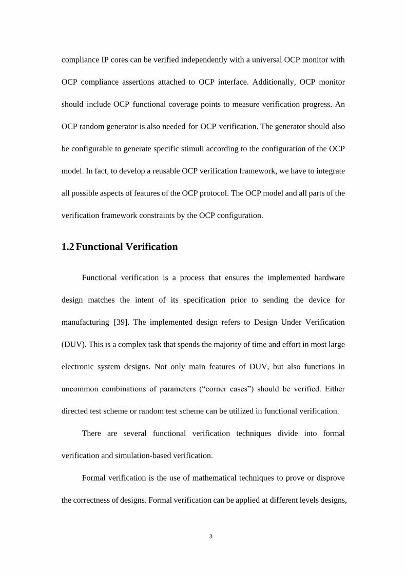
the hardware design phase itself, but the verification of it [13]. It was noticed that
verification takes around 60% to 80% of chip development effort in terms of time.
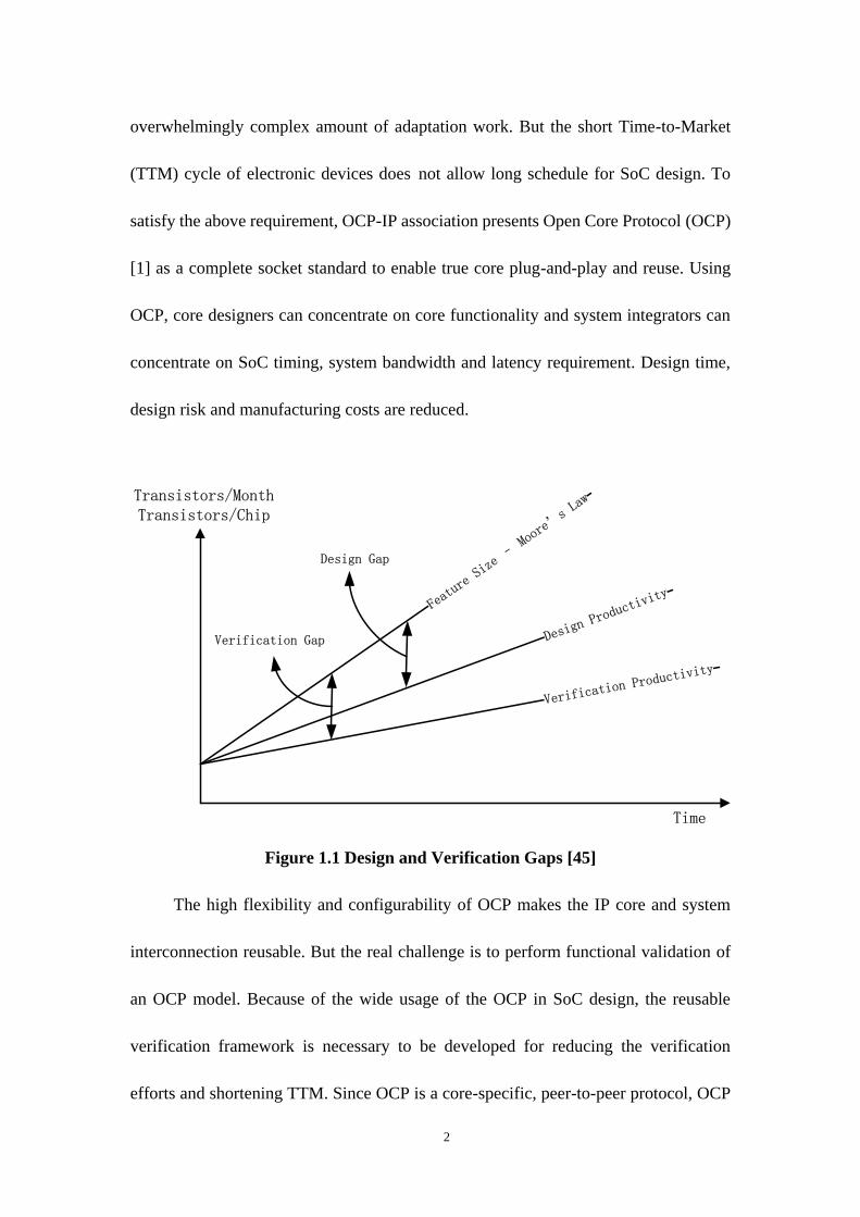
Figure 1.1 shows the design and verification gaps.
Thousands of Intellectual Property (IP) cores and hundreds of hardware
interconnects or buses have been involved SoC design. Tens even hundreds of IP cores
can be integrated into a chip to provide various functions. For different SoC designs, IP
cores have to be readapted to different interconnects. This makes SoC design an
2
overwhelmingly complex amount of adaptation work. But the short Time-to-Market
(TTM) cycle of electronic devices does not allow long schedule for SoC design. To
satisfy the above requirement, OCP-IP association presents Open Core Protocol (OCP)
[1] as a complete socket standard to enable true core plug-and-play and reuse. Using
OCP, core designers can concentrate on core functionality and system integrators can
concentrate on SoC timing, system bandwidth and latency requirement. Design time,
design risk and manufacturing costs are reduced.
Figure 1.1 Design and Verification Gaps [45]
The high flexibility and configurability of OCP makes the IP core and system
interconnection reusable. But the real challenge is to perform functional validation of
an OCP model. Because of the wide usage of the OCP in SoC design, the reusable
verification framework is necessary to be developed for reducing the verification
efforts and shortening TTM. Since OCP is a core-specific, peer-to-peer protocol, OCP
Time
Transistors/MonthTransistors/Chip
Verification
Productivit
y
Design
Produ
ctivit
yFeature Size –
Moore’s Law
Verification Gap
Design Gap
3
compliance IP cores can be verified independently with a universal OCP monitor with
OCP compliance assertions attached to OCP interface. Additionally, OCP monitor
should include OCP functional coverage points to measure verification progress. An
OCP random generator is also needed for OCP verification. The generator should also
be configurable to generate specific stimuli according to the configuration of the OCP
model. In fact, to develop a reusable OCP verification framework, we have to integrate
all possible aspects of features of the OCP protocol. The OCP model and all parts of the
verification framework constraints by the OCP configuration.
1.2 Functional Verification
Functional verification is a process that ensures the implemented hardware
design matches the intent of its specification prior to sending the device for
manufacturing [39]. The implemented design refers to Design Under Verification
(DUV). This is a complex task that spends the majority of time and effort in most large
electronic system designs. Not only main features of DUV, but also functions in
uncommon combinations of parameters (“corner cases”) should be verified. Either
directed test scheme or random test scheme can be utilized in functional verification.
There are several functional verification techniques divide into formal
verification and simulation-based verification.
Formal verification is the use of mathematical techniques to prove or disprove
the correctness of designs. Formal verification can be applied at different levels designs,
4
ranging from gate-level to Register Transfer Level (RTL). Main techniques of the
formal verification method are Equivalence Checking, Model Checking and Theorem
Proving [2]. Equivalence checking is a formal, static verification technology which
uses mathematical techniques to determine if two versions of the same design that are
designed by different abstraction levels are functionality equivalent. The two versions
could be two RTL versions, an RTL description and a gate-level netlist and two
gate-level netlists. Model checking is an automatic technique for verifying finite state
concurrent systems, such as digital circuits and communication protocol. The
procedure uses an exhaustive search of the state space of the system to find out whether
some specification is true or not. The procedure can terminate with a yes/no answer
with a given sufficient resources. Although the disadvantage of model checking is the
restriction on finite state systems, it is used on several important types of systems such
as hardware controller and many communication protocols. Additionally, in some cases
bugs can be found by restricting unbounded data structure to specific finite state
instances. Model checking is preferable to deductive verification because it can be
performed automatically. But some critical applications are necessary to be verified
completely by theorem proving. Theorem Proving (deductive verification) refers to the
use of axioms and proof rules to prove the correctness of the systems. It is a
time-consuming process that can be performed only by experts who are educated in
logic reasoning and have considerable experience. It can spend days or months to prove
a single protocol or circuit. So theorem proving is used rarely and applied primarily to
5
highly sensitive systems such as security protocols. Some mathematical tasks cannot be
performed by an algorithm. Because there cannot be an algorithm that decides whether
an arbitrary computer program terminates, correct termination of programs cannot be
verified automatically in general. Therefore, most proof system cannot be completely
automated. The main high order logic provers are HOL [3] and PVS [4].
Simulation-Based Verification, also called dynamic verification, is widely used
in hardware verification. A testbench is built to provide meaningful scenarios to verify
the logic behavior of the hardware design. A testbench can provide random, directed
and constrained random stimuli over the entire input space of the DUV. A testbench is
typically composed of the several types of verification components. Data Item
represents the input of the DUV. Examples include bus transactions, networking
packets and CPU instructions. A Driver repeatedly receives a data item and drives it to
the DUV by sampling and driver the DUV signals. A Sequencer is an advanced
stimulus generator that controls the data items that are provided to the driver for
execution. Constraints can be added in order to control the distribution of randomized
value. A Monitor is a passive entity that samples DUV signals but does not drive them.
Monitors collect coverage information and perform protocol and data checking.
Sequencer, driver and monitor can be reused independently. An Agent works as an
abstract container to encapsulate a driver, sequencer and monitor. The Environment is
the top-level component of the testbench which contains one or more agents. Some
reusable frameworks for verification components, such as VMM [5], AVM [6] and
6
OVM [7], have been provided by different EDA companies.
There are different verification methodologies including Assertion-Based
Verification (ABV), Coverage-Driven Verification (CDV) and Metric-Driven
Verification (MDV).
In ABV, assertions are quite simply design checks embedded in the module or IP
to capture specific design intent and verify that the design correctly implements that
intent either through simulation or formal verification. There are two types of assertions:
Concurrent Assertions and Immediate Assertions [8]. Concurrent assertions express
behavior spans over time. They are evaluated only at the occurrence of a clock tick.
Concurrent assertions can be used with both formal and simulation-based verification.
Immediate assertions are based on event semantics. Unlike concurrent assertions,
immediate assertions are not temporal in nature and are evaluated immediately. They
are used only with dynamic simulation. Assertion statements are written by HDL or
special assertion languages such as SystemVerilog Assertion (SVA) [9], OpenVera
Assertion (OVA) [10] and Property Specification Language (PSL) [11].
Coverage-driven verification combines automatic test generation, self-checking
testbench and coverage metrics to significantly reduce the time spent verifying a design
[7]. The CDV starts by setting verification goal using an organized planning process.
Then a smart testbench is created to generate and send stimuli to the DUV. A monitor is
connected to measure coverage process and identify undesired DUV behavior. The
verification is ended when the verification goal has been achieved. Coverage metrics
7
includes code coverage, finite state machine coverage, structural coverage and
functional coverage.
Metric-Driven Verification improves coverage-driven verification approach by
making the verification plan in an executable format. The executable verification plan
can be used directly to generate verification scenarios, measure verification progress
and identify verification closure.
1.3 Coverage Directed Test Generation
The functional specification of DUV can be translated to functional coverage
tasks in SoC verification. Two steps are employed to the functional coverage process:
(1) Define the cover points; (2) Finding meaningful stimuli to cover those points [12].
This process which is called Coverage Directed-test Generation (CDG) is repeated
until the exit criteria (verification goals) are met.
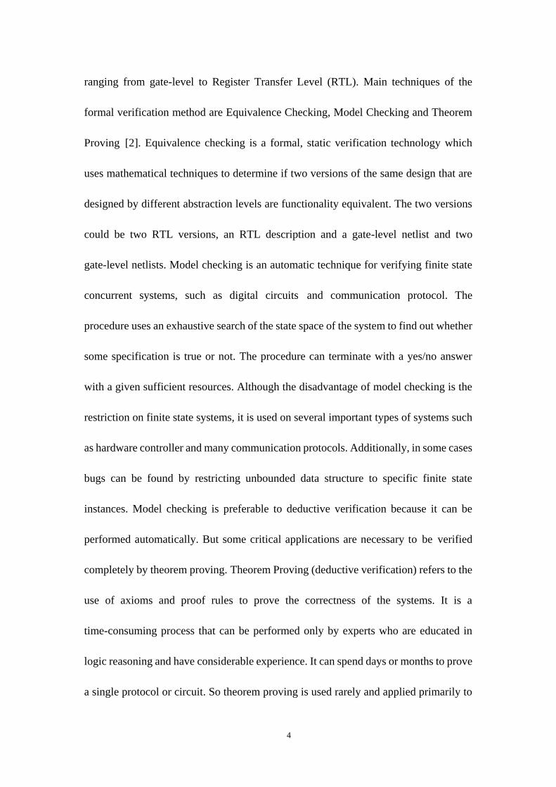
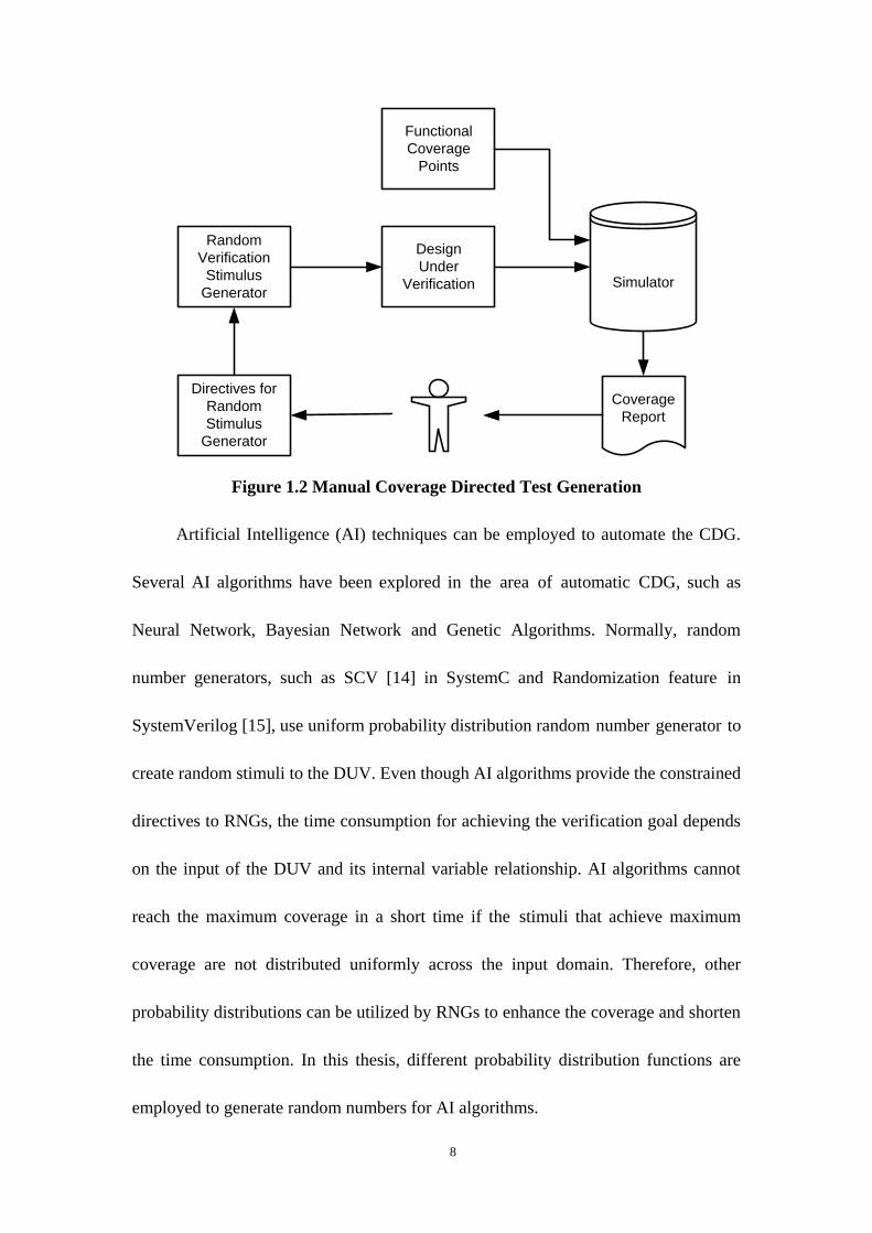
Figure 1.2 shows the manual CDG where verification engineers guide the
random number generator by setting up directives and constraints. The manual effort of
analyzing the coverage reports and translating them to directives for Random Number
Generator (RNG) can constitute a bottleneck in the verification process. Therefore, it is
worth to spend considerable effort on finding a method to automate this procedure and
close the loop of coverage analysis and test generation. The automated CDG can
dramatically reduce the manual effort in the verification process and increase its
efficiency.
8
Figure 1.2 Manual Coverage Directed Test Generation
Artificial Intelligence (AI) techniques can be employed to automate the CDG.
Several AI algorithms have been explored in the area of automatic CDG, such as
Neural Network, Bayesian Network and Genetic Algorithms. Normally, random
number generators, such as SCV [14] in SystemC and Randomization feature in
SystemVerilog [15], use uniform probability distribution random number generator to
create random stimuli to the DUV. Even though AI algorithms provide the constrained
directives to RNGs, the time consumption for achieving the verification goal depends
on the input of the DUV and its internal variable relationship. AI algorithms cannot
reach the maximum coverage in a short time if the stimuli that achieve maximum
coverage are not distributed uniformly across the input domain. Therefore, other
probability distributions can be utilized by RNGs to enhance the coverage and shorten
the time consumption. In this thesis, different probability distribution functions are
employed to generate random numbers for AI algorithms.
Simulator
Random
Verification
Stimulus
Generator
Directives for
Random
Stimulus
Generator
Design
Under
Verification
Functional
Coverage
Points
Coverage
Report
9
1.4 Related Work
In this section, we present the related work in the area of assertion-based
verification methodology for OCP TLM models. Then we give some methodologies for
verifying the correctness of RTL refinement from TLM modeling. Then we will focus
on functional coverage-based verification methodologies and algorithms such as
Bayesian Network, Neural Network and Genetic Algorithm. Finally, we present a
methodology of cell-based genetic algorithm with different probability distributions
that is utilized to automate coverage directed test generation.
Many considerable efforts have been spent on OCP TLM verification in ABV. In
[18], because the DUV is SystemC model, the authors developed a native assertion
mechanism „NSCa‟ in SystemC in order to employ their verification process. NSCa can
construct a cycle level accuracy rule of the design as assertion expression form. The key
variation in our approach is the formation of our assertion suite. Our scheme is based
on off the shelf SVA which does not need any tailored SystemC based assertions. In
addition, since SystemVerilog Assertions has a wider acceptance as an assertion
language our approach stands elevated. Another work [19] focused on an
assertion-based approach for system-level performance analysis applied to the
single-channel OCP system. The system was described with SystemC TLM and in the
analysis approach; performance primitives such as data rate and transaction latency
were described using the Transaction Level Assertion (TLA). The prime difference
between our research and the above mentioned research is in the method to construct of
10
Re-Usable Assertions for design models created in various abstraction levels. Our
assertion structure seamlessly integrates not only with models described at Transaction
Level (TLM) but also with models written at Register Transfer Level (RTL).
Therefore, our assertion suite minimizes the Design-Verification phase and enhances
Time-to-Market factor.
Several attempts have been made to automate CDG. In [20], Bayesian Network
is employed to model the relationship between coverage tasks space and the directives
of a random test generator. This approach includes two phases: Learning phase and
Evaluation phase. In the learning phase, a Bayesian network is constructed to
represent the relationship between the coverage tasks and the test generation
directives. Then a set of sample directives are used to run simulations and obtain a set
of coverage results respectively. After that, a learning algorithm can be applied to
estimate the parameters of the Bayesian network. In the evaluation phase, the trained
Bayesian network can be used to generate directives for desired coverage tasks. The
disadvantage of this approach is that the quality of certain sample directives has great
influence on the ability of the Bayesian network to generate efficient test generation
directives. In contrast, the CGA which is employed in this thesis starts with random
number initiation and the quality of the initiation only affects the speed of evolution
but not the quality of the generation. Artificial Neural Networks (ANNs) [44] are
utilized to solve the Priority Directed test Generation (PDG) problems in the work of
[21]. The DUV (OR1200 RISC CUP) was targeted by several directed test vectors.
11
The coverage result was represented by identified rate of predefined bugs for every
test vector. Then the ANN was used to analyze the coverage results and determine the
priority of each vector. Finally, the predefined test vectors with high priority can be
reused for further verifications. This algorithm uses predefined test vectors with
different priorities instead of random initialization in our CGA generator.
Genetic Algorithm has been employed to optimize the input test vectors in
several functional verification methodologies. A simple genetic algorithm is introduced
to guide random input sequences for improving coverage count of property checks in
[22]. But this work can target only one property at a time. Moreover, it cannot describe
sharp constrains on random inputs. In [23], a genetic algorithm is utilized to generate
biased random instructions automatically for microprocessor architecture RTL model
verification. The averages utilization statistics of specific buffers in PowerPC
architecture are defined as coverage metrics. This approach is only for microprocessor
verification. In contrast, our OCP verification framework is reusable for all
OCP-compliance IP cores or bus interfaces. The work of [24] introduced genetic
algorithm into a reusable verification environment. The environment adopts layered
architecture and includes five layers: Signal layer, Command layer, Function layer,
Scenario layer and Test layer. Only three chromosomes were initialized at the
beginning of the simulation. In our framework, the initialization size of the CGA can
be predefined and represent more complex solution.
The work of [12] provided a Cell-based Genetic Algorithm (CGA) to automate
12
CDG. The CGA divided the input domain into sequences of inputs called cells. Each
cell is represented by three parameters: upper limit, lower limit and weight. The
number of cells and the range of the input domain are configured according to the DUV
by the user. The process of the CGA begins from generating a certain number of cells
randomly. Each cell targets the DUV and the coverage information of the cell is
collected by the simulator. Then, the quality of each cell is evaluated by a predefined
evaluation function which is called fitness function. Based on predefined criteria, the
cells with good quality are preserved and forwarded to the next generation. The rest of
the cells are modified by genetic operations for the new generation. Only uniform
random generator is utilized in CGA. The work of [25] enhanced the CGA by adding
several random number generators which are based on different probability
distributions. The approach is applied to a SystemC 16×16 packet switch RTL model
with several coverage points. The experiment results show that some RNGs based on
specific probability distributions get greater fitness value within smaller number of
generations than others. In this thesis, the CGA is employed to verify higher abstraction
level TLM models instead of RTL models. The generation with the best coverage
quality should be reused in RTL models.
1.5 OCP Verification Methodology
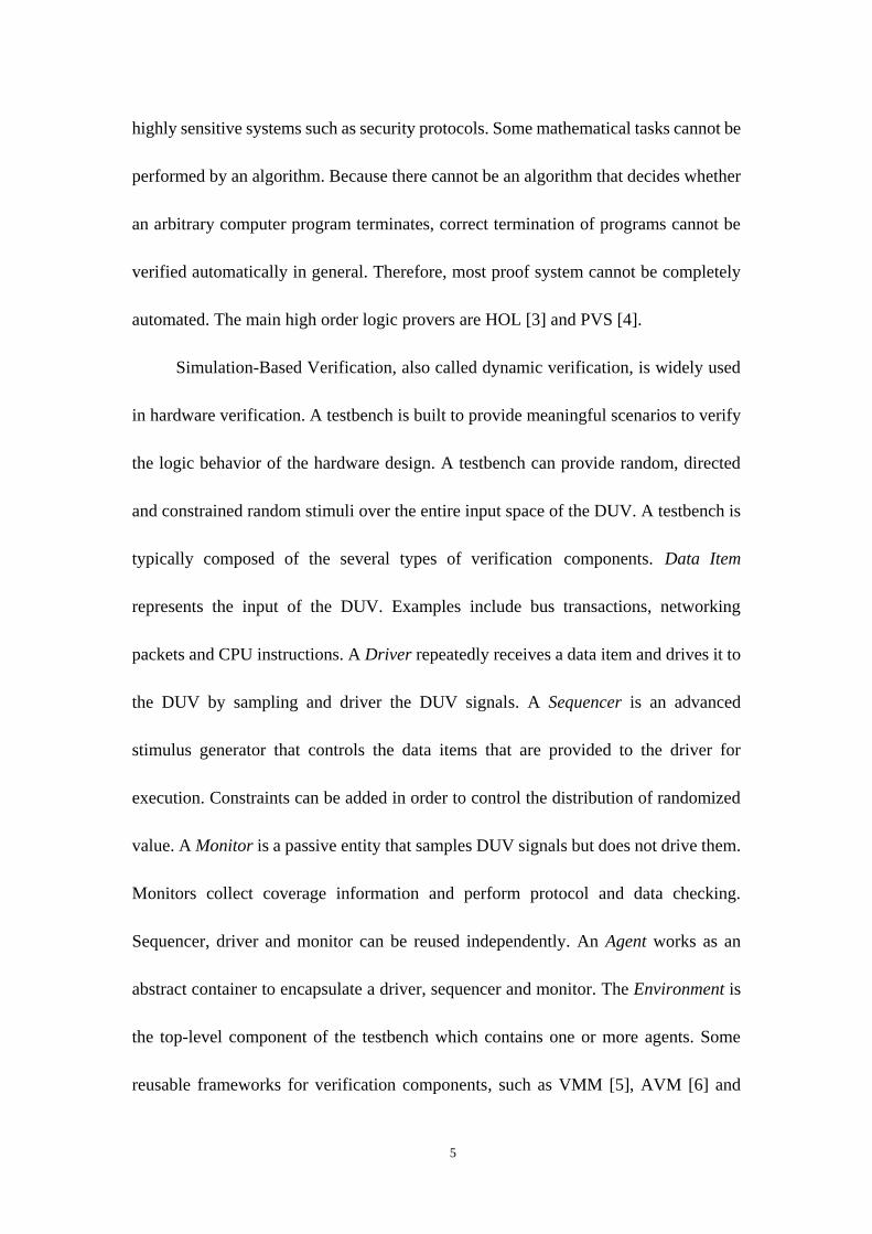
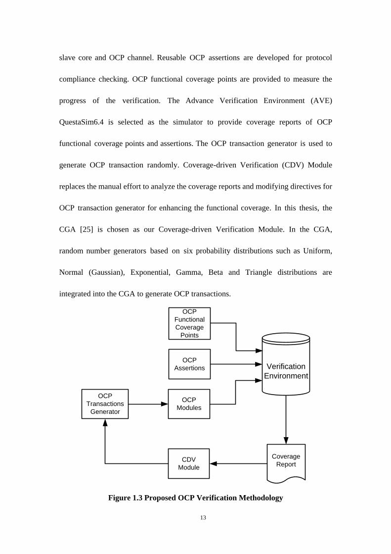
Figure 1.3 depicts our proposed OCP verification methodology. The DUV is an
OCP model which normally includes different abstraction level of OCP master core,
13
slave core and OCP channel. Reusable OCP assertions are developed for protocol
compliance checking. OCP functional coverage points are provided to measure the
progress of the verification. The Advance Verification Environment (AVE)
QuestaSim6.4 is selected as the simulator to provide coverage reports of OCP
functional coverage points and assertions. The OCP transaction generator is used to
generate OCP transaction randomly. Coverage-driven Verification (CDV) Module
replaces the manual effort to analyze the coverage reports and modifying directives for
OCP transaction generator for enhancing the functional coverage. In this thesis, the
CGA [25] is chosen as our Coverage-driven Verification Module. In the CGA,
random number generators based on six probability distributions such as Uniform,
Normal (Gaussian), Exponential, Gamma, Beta and Triangle distributions are
integrated into the CGA to generate OCP transactions.
Figure 1.3 Proposed OCP Verification Methodology
OCP
Modules
Verification
Environment
Coverage
Report
OCP
Assertions
OCP
Transactions
Generator
CDV
Module
OCP
Functional
Coverage
Points
14
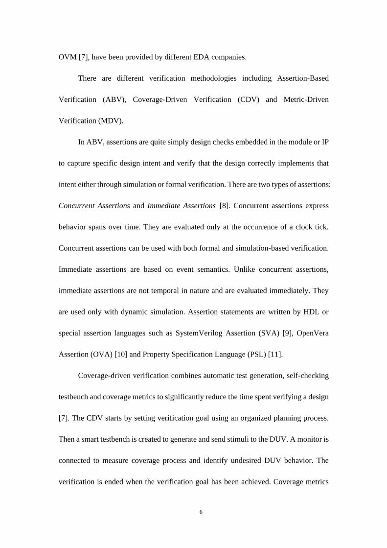
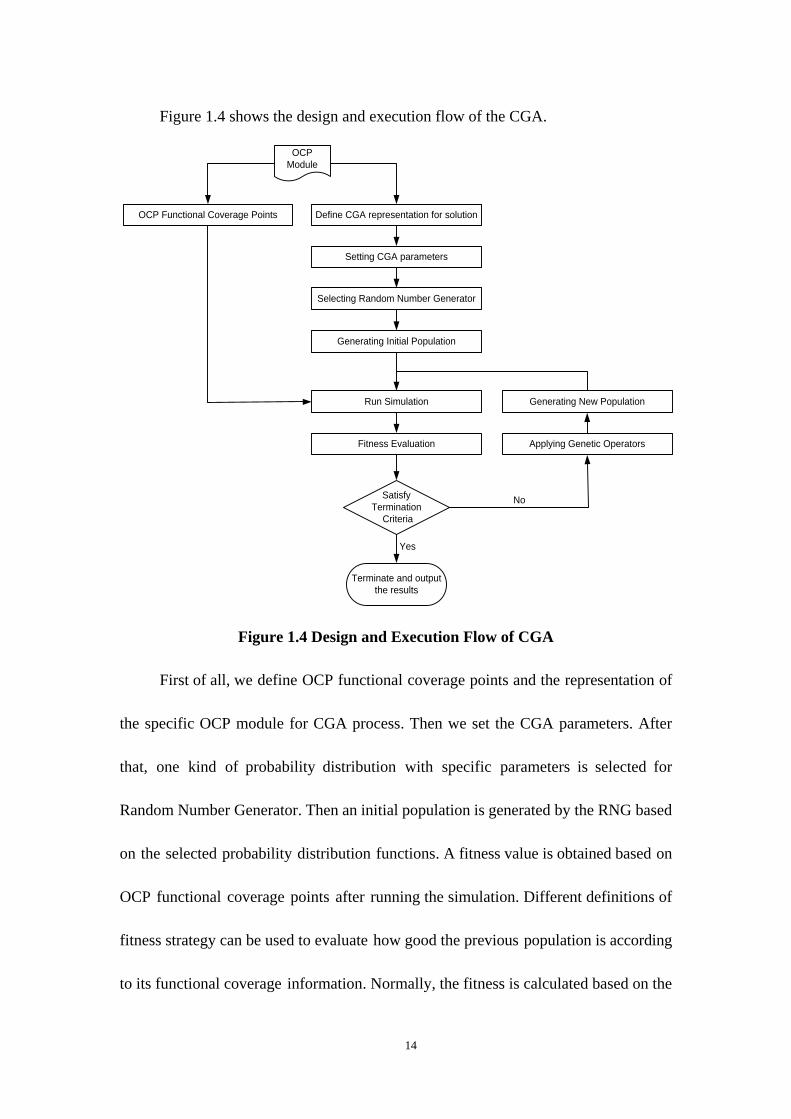
Figure 1.4 shows the design and execution flow of the CGA.
Figure 1.4 Design and Execution Flow of CGA
First of all, we define OCP functional coverage points and the representation of
the specific OCP module for CGA process. Then we set the CGA parameters. After
that, one kind of probability distribution with specific parameters is selected for
Random Number Generator. Then an initial population is generated by the RNG based
on the selected probability distribution functions. A fitness value is obtained based on
OCP functional coverage points after running the simulation. Different definitions of
fitness strategy can be used to evaluate how good the previous population is according
to its functional coverage information. Normally, the fitness is calculated based on the
OCP
Module
Define CGA representation for solution
Satisfy
Termination
Criteria
Terminate and output
the results
Setting CGA parameters
Selecting Random Number Generator
Generating Initial Population
Run Simulation
Fitness Evaluation
Generating New Population
Applying Genetic Operators
Yes
No
OCP Functional Coverage Points
15
percentage of the cover points being hit over the total number of coverage points in the
DUV. The fitness evaluation guides the next generation of the process. Some of the
elements with good quality in the population are forwarded or preserved to perform
genetic operations such as crossover, mutation to the new population. The remaining
part of the new population is filled by new random number generation. The whole
evolution process is performed until the given termination criteria is reached.
1.6 Thesis Contribution and Organization
In light of the above related work review and discussions, we believe the
contributions of this thesis are as follows:
A set of OCP assertions in SystemVerilog Assertion (SVA) for protocol
compliance checking have been defined.
A reusable OCP verification framework for different abstraction levels
(TLM and RTL) OCP models has been developed.
A Cell-based Genetic Algorithm (CGA) using different probability
distribution RNGs on different OCP TL1 channel models to enhance their
functional coverage automatically has been implemented.
A random generator has been defined in SCV and the results have been
compared to the CGA approach.
The rest of the thesis is organized as following. Chapter 2 provides an
introduction of Open Core Protocol. Then we present the basic principles and operators
16
of the genetic algorithms. We also provide overviews of SystemC and SystemVerilog
language and formulas of different probability distributions. This chapter lays a
foundation for the better understanding of the thesis. Chapter 3 presents our reusable
OCP verification methodology. OCP TL1 channel models are selected as DUVs to be
verified by directed tests and random tests. The proposed CGA based on different
probability distribution RNGs is utilized to enhance the OCP functional coverage. To
compare with the CGA, SCV random generators are employed to generate OCP
random transactions as well. An OCP monitor with SVA assertions is attached to OCP
channel for protocol checking. In Chapter 4, the implementation results of both directed
tests and random tests are presented. We also describe functional coverage points
which are defined in SystemC and SystemVerilog for SCV and CGA simulations
respectively. After that, we discuss about the experiment results of CGA and SCV.
Finally, we present our conclusion and some possible future works.

Chapter 2
Preliminary
This chapter describes briefly the preliminary components on which we are
going to build our work in this thesis. They are Open Core Protocol, Genetic
Algorithm, SystemC, SystemVerilog and probability distribution functions.
2.1 Open Core Protocol
Open Core Protocol (OCP) [1] is a non-profit, open standard protocol that
facilitates IP cores reuse and SoC integration. It defines a high performance,
bus-independent interface between IP cores and it suits all hardware behaviors.
Because of its high flexibility and configurability, OCP can be configured for high
performance microprocessor, DMA blocks with out-of-order and outstanding
transactions, simple peripheral core and on-chip communication subsystem. SoC
designers can tailor the best OCP configuration socket with require features only for
each IP core.
An OCP module is comprised of three parts: OCP Master Core, OCP Slave
Core and OCP Channel (OCP interface). The OCP Channel is a points-to-point
interface for two communication entities such as IP cores and bus interface modules.
One of the entities is the OCP master core, and the other is the OCP slave core. The
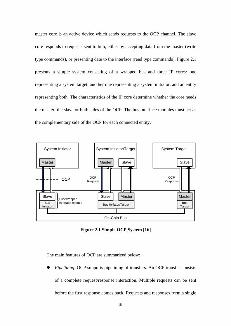
18
master core is an active device which sends requests to the OCP channel. The slave
core responds to requests sent to him, either by accepting data from the master (write
type commands), or presenting date to the interface (read type commands). Figure 2.1
presents a simple system consisting of a wrapped bus and three IP cores: one
representing a system target, another one representing a system initiator, and an entity
representing both. The characteristics of the IP core determine whether the core needs
the master, the slave or both sides of the OCP. The bus interface modules must act as
the complementary side of the OCP for each connected entity.
Figure 2.1 Simple OCP System [16]
The main features of OCP are summarized below:
Pipelining: OCP supports pipelining of transfers. An OCP transfer consists
of a complete request/response interaction. Multiple requests can be sent
before the first response comes back. Requests and responses form a single
System Initiator
Master
System Initiator/Target
Master
System Target
SlaveSlave
On-Chip Bus
Slave Slave Master Master
Bus
InitiatorBus Initiator/Target
Bus
Target
OCPOCP
Request
OCP
Response
Bus wrapper
interface module
19
ordered thread and responses must be returned in the order of the requests.
Data handshake: OCP master sends request and data separately with the data
handshake signals instead of sending them together. To support data
handshake feature, we can simply set OCP parameter datahandshake to 1.
Threads: OCP interface can proceed to multiple transfers concurrently and
out-of-order. OCP transfers in different threads have no ordering property
and can be implemented independently in different control flows. To support
multi threads feature, we set OCP parameter threads greater than 1.
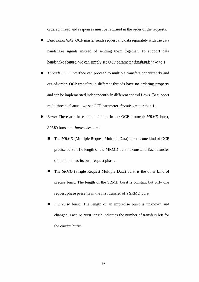
Burst: There are three kinds of burst in the OCP protocol: MRMD burst,
SRMD burst and Imprecise burst.
The MRMD (Multiple Request Multiple Data) burst is one kind of OCP
precise burst. The length of the MRMD burst is constant. Each transfer
of the burst has its own request phase.
The SRMD (Single Request Multiple Data) burst is the other kind of
precise burst. The length of the SRMD burst is constant but only one
request phase presents in the first transfer of a SRMD burst.
Imprecise burst: The length of an imprecise burst is unknown and
changed. Each MBurstLength indicates the number of transfers left for
the current burst.
20
2.2 Genetic Algorithm
Genetic Algorithms (GAs) [26] are adaptive heuristic search techniques which
were first invented by John Holland in the 1960s. As a particular class of evolutionary
algorithm (EA), it follows Charles Darwin‟s principals of survival of the fittest to
simulate process in nature evolution and generate high quality solutions to search and
optimize problems. A genetic algorithm is an iterative procedure implemented in a
computer simulation. During the simulation, a population of an abstract artificial
representation is initialized and evaluated at first. Then some part of the solution with
good quality will be kept and forwarded to the next population. This evolution process
will run continuously until a satisfactory solution is found. Genetic algorithms cannot
guarantee a unique best solution, but it finds optimal solutions more efficiently than
traditional search techniques (linear programming [27], depth-first search (DFS) [28],
breadth-first search (BFS) [29], etc.) in optimizing search problems with large space.
Therefore, genetic algorithms have been studied, experimented and applied in many
fields of science and engineering.
A typical GA needs a genetic representation and a fitness function. Genetic
representation is used to represent solutions/individuals of the problems. Individuals of
the problem are represented in binary arrays or other encoding methods (trees, hashes,
etc.). As shown in Figure 2.2, the individual is called chromosome or genome.
Potential individuals make up a population. The size of the population rests on the
complexity of the search problem and the size of the search space. In generally, the size
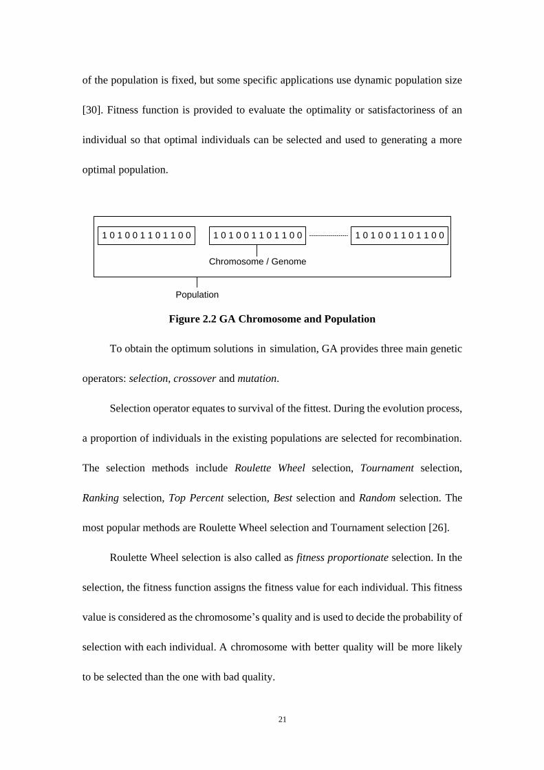
21
of the population is fixed, but some specific applications use dynamic population size
[30]. Fitness function is provided to evaluate the optimality or satisfactoriness of an
individual so that optimal individuals can be selected and used to generating a more
optimal population.
Figure 2.2 GA Chromosome and Population
To obtain the optimum solutions in simulation, GA provides three main genetic
operators: selection, crossover and mutation.
Selection operator equates to survival of the fittest. During the evolution process,
a proportion of individuals in the existing populations are selected for recombination.
The selection methods include Roulette Wheel selection, Tournament selection,
Ranking selection, Top Percent selection, Best selection and Random selection. The
most popular methods are Roulette Wheel selection and Tournament selection [26].
Roulette Wheel selection is also called as fitness proportionate selection. In the
selection, the fitness function assigns the fitness value for each individual. This fitness
value is considered as the chromosome‟s quality and is used to decide the probability of
selection with each individual. A chromosome with better quality will be more likely
to be selected than the one with bad quality.
1 0 1 0 0 1 1 0 1 1 0 0 1 0 1 0 0 1 1 0 1 1 0 0 1 0 1 0 0 1 1 0 1 1 0 0
Chromosome / Genome
Population
22
In tournament selection method, a “tournament size” of individuals is chosen
from a population randomly. Then, the best one in the chosen individuals will be
selected for the new offspring. It is easy to adjust the selection pressure by changing the
tournament size. Weak individuals have a small chance to be selected in a large size
tournament. But the problem of the tournament selection method is that the best
individual may have no chance to be kept for the next generation if it is not in the
tournament. Elitism addresses this problem by copy the best individual to the elitism
set. Individuals in the elitism set are preserved for the evolution process and are never
changed by genetic operators.
After applying selection operator, the selected individuals can be kept and
forwarded to the next population directly or through crossover and/or mutation
operators.
Crossover operator is employed between two selected individuals by exchanging
parts of their genome to create new individuals. It is useful to preserve and forwards
good features of exist individuals to the next generation. There are many different kinds
of crossover methods, the most common types are one-point crossover and two-point
crossover. Figure 2.3 illustrates them respectively. Crossover is performed with a set
probability. If no crossover occurs, the selected individuals are copied to the new
generation directly.

23
Figure 2.3 Crossover Operators
After selection and crossover, mutation operator is performed to change an
arbitrary bit or bit-string in current individual as Figure 2.4 illustrates. The bits are
chosen randomly. The purpose of mutation operator in GA is to avoid slowing
evolution by preventing individuals from becoming too similar to each other.
Figure 2.4 Mutation Operator
Normally, a GA evolution process includes the following steps:
Initialize a population (n) randomly
Calculate the fitness of the population (n).
Repeat until termination:
Select a proportion of existing population (n) to produce the new
population (n+1)
Perform crossover and mutation operators to generate the new
1 0 1 0 0 1 1 0 1 1 0 0
0 0 1 1 0 1 1 1 0 1 0 1
0 0 1 1 0 1 1 0 1 1 0 0
1 0 1 0 0 1 1 1 0 1 0 1
Single Point Crossover
1 0 1 0 0 1 1 0 1 1 0 0
0 0 1 1 0 1 1 1 0 1 0 1
0 0 1 0 0 1 1 0 1 1 0 1
1 0 1 1 0 1 1 1 0 1 0 0
Two Points Crossover
1 0 1 0 0 1 1 0 1 1 0 0 1 0 1 0 0 0 1 0 1 1 0 0 Mutation
Operator
24
population (n+1)
Calculate the fitness of the population (n+1)
Terminate due to obtain a satisfactory solution or a maximum number of
generations have been reached
First of all, the GA process starts by initializing a random population.
Traditionally, the initial population is produced randomly, but it can be generated using
some optimal algorithms that are easy to be found. After the initialization, the quality
(fitness value) of the population is calculated by the fitness function. Then the
population is evolved by three GA operators: selection, crossover and mutation to
generate new populations repeatedly until a satisfactory solution has been obtained or
the maximum number of generation have been reached.
2.3 SystemC Language
SystemC [31] is an open-source language based on C++. It is both a system level
and hardware description language [32]. It is a hardware description language because
SystemC allows register transfer level (RTL) modeling. It is a system level
specification language because it supports high abstraction level (TLM or System
Level) modeling. SystemC does not add new syntax to C++ programming language.
Actually, SystemC is a new C++class library which provides powerful new mechanism
to model system architecture with hardware timing, concurrency and reactive behavior.
25
2.3.1 SystemC Architecture
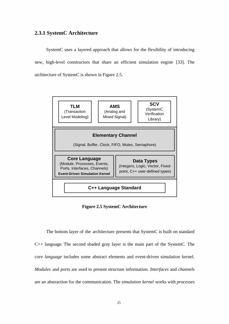
SystemC uses a layered approach that allows for the flexibility of introducing
new, high-level constructors that share an efficient simulation engine [33]. The
architecture of SystemC is shown in Figure 2.5.
Figure 2.5 SystemC Architecture
The bottom layer of the architecture presents that SystemC is built on standard
C++ language. The second shaded gray layer is the main part of the SystemC. The
core language includes some abstract elements and event-driven simulation kernel.
Modules and ports are used to present structure information. Interfaces and channels
are an abstraction for the communication. The simulation kernel works with processes
C++ Language Standard
Core Language(Module, Processes, Events,
Ports, Interfaces, Channels)
Event-Driven Simulation Kernel
Elementary Channel
(Signal, Buffer, Clock, FIFO, Mutex, Semaphore)
TLM(Transaction
Level Modeling)
AMS(Analog and
Mixed Signal)
SCV(SystemC
Verification
Library)
Data Types(Integers, Logic, Vector, Fixed-
point, C++ user-defined types)
26
and events during the simulation. It does not know what the events actually represent
or what the processes do. It only operates on events and switches between processes.
On the right side of the core language, a set of data types can be used to model
hardware and program software. The elementary channel layer is immediately above
the core language. The elementary channels such as signals, buffers and FIFOs are
widely used in hardware modeling. On the top of the architecture, the layers of extend
design and methodology libraries are considered separate from the SystemC standard.
Some of the extend libraries, such as SCV, AMS and TLM, are widely used in
hardware design and verification. Over time, new libraries may be added and
conceivably be incorporated into the standard language.
2.3.2 Transaction Level Modeling in SystemC
Transaction Level Modeling (TLM) is a design and verification abstraction
above RTL. It provides an early platform for software development so that software can
be designed very early in the design flow. TLM abstracts hardware implementation
details and uses function calls to model the communication between blocks in the
system, and therefore it is much faster than RTL modeling. Additionally, designers can
modify and replace the IP cores and buses more easily than RTL in system level design
exploration and verification. TLM increases the productivity of software engineer,
architects, implementation engineers and verification engineers.
Open SystemC Initiative (OSCI) released standard SystemC TLM library [35]. It
provides a valuable set of templates and implementation rules for standardizing TLM
27
methodology. In fact, transaction level does not denote a single level of description.
Rather, it refers to a group of three abstraction levels. Programmer‟s View (PV) level is
the highest level which is widely used by programmers. There is no hardware timing
information in PV level. Programmer‟s View plus Timing (PVT) level enriches PV
level with approximately timing information. It can be used for preliminary
performance analysis. The lowest level is the Cycle Accurate (CA) level which adds
the hardware design notion of clock and describes what happens at each clock cycle.
Although CA level is cycle accurate, it is still faster RTL.
2.3.3 SCV
The SystemC standard can only be used to perform basic verification of a design.
The SystemC Verification Working Group (SVWG) has identified the applicable
verification requirements, discussed proposals from various members and provided the
SystemC Verification Standard (SCV) as a set of features to be incorporated into the
SystemC Standard [14]. SCV improves the capability of SystemC by adding APIs for
transaction-based verification, constraint and weighted randomization, exception
handling and other verification tasks. The main items within the SCV are as following:
transaction-based verification
data introspection
constraint and weighted randomization
transaction monitoring and recording

28
2.4 SystemVerilog
IEEE-1800, SystemVerilog [34] extends Verilog-2001 by adding important new
features for design, synthesis and verification. The extensions include simple
enhancements to existing constructs, extensions of data types and operators, a new
constructs of Object-Oriented mechanism, assertion mechanism for verifying design
intent and so forth.
As the integral part of SystemVerilog, SystemVerilog Assertions (SVA) is used
for the temporal aspects of specification, modeling and verification. It can embed
sophisticated assertions and functional checks in HDL code. It can also allow simple
boolean expressions into complex definitions of design behavior.
2.5 Probability Distribution
In probability theory and statistics, a probability distribution describes
probabilities that a random variable can take within all possible values. There are two
types of probability distribution functions: continuous probability distribution
functions and distribution probability distribution functions. A discrete probability
distribution function gives a discrete number of values and their certain probabilities
of occurrence at random events. The common discrete distributions are Binomial
distribution, Geometric distribution, Logarithmic distribution and Poisson distribution
[36]. Unlike discrete probability distributions, a continuous probability density
function (PDF) measure the probability of an infinite number of values over
29
continuous interval and the probability of each single value is always zero in
continuous PDF. The main PDFs include Uniform distribution, Normal distribution,
Beta distribution, Gamma distribution, Exponential distribution, Rice distribution,
Triangular distribution, Lognormal distribution and Weibull distribution [36]. In this
thesis, six continuous probability distributions are selected for generating random
number in CGA, their probability density functions are presented as follows.
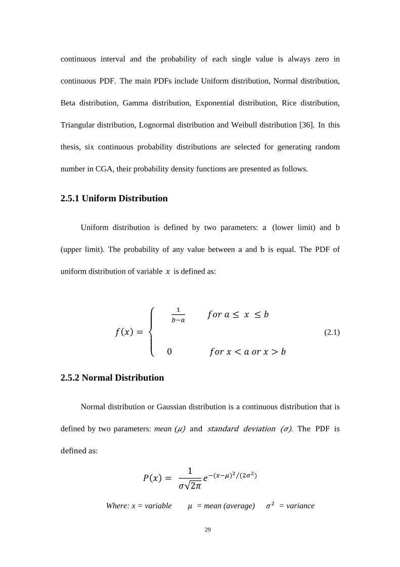
2.5.1 Uniform Distribution
Uniform distribution is defined by two parameters: (lower limit) and
(upper limit). The probability of any value between and is equal. The PDF of
uniform distribution of variable is defined as:
(2.1)
2.5.2 Normal Distribution
Normal distribution or Gaussian distribution is a continuous distribution that is
defined by two parameters: mean ( ) and standard deviation ( ). The PDF is
defined as:
Where: x = variable = mean (average) = variance
30
2.5.3 Exponential Distribution
The PDF of Exponential distribution is defined as:
(2.3)
Where: > 0 and x (1, )
2.5.4 Beta Distribution
Beta distribution is another continuous distribution that is defined by two parameters:
and . The PDF is defined as:
(2.4)
Where: 0< x< 1
2.5.5 Gamma Distribution
Gamma distribution is a non-symmetric continuous probability distribution that has
two parameters: scale factor and shape factor . The PDF is defined as:
(2.5)
Where: k and > 0

31
2.5.6 Triangle Distribution
Triangle distribution is defined by three parameters: low limit, mode, and upper limit.
The PDF is given in the equation.
(2.6)
Chapter 3
OCP Verification Methodologies
In this chapter, we provide both directed test scheme and random test scheme to
verify OCP modules. In directed test scheme, a reusable OCP verification framework
is developed to verify both TLM and RTL OCP models. After that, we employ SCV
as a pure random number generator to generate OCP transactions to OCP TLM
modules. Finally, we present the proposed methodology that utilizing Cell-based
Genetic Algorithm with multiple probability distribution random number generators to
generate OCP transactions and enhance the functional coverage of the OCP TLM
models.
3.1 Reusable OCP TLM Verification Environment
Figure 3.1 depicts the proposed verification methodology. The DUV (Design
Under Verification) includes OCP generic master core, OCP generic slave core and
OCP TLM (Cycle-Accurate Level) channel. The master and the slave cores are
attached to one side of the OCP TL1 channel respectively. They communicate with
each other by the channel. During the simulation, the master gets OCP requests from
directed request tables and then sends the requests to the slave. The slave receives the
requests and returns the corresponding responses to the master. An implementing
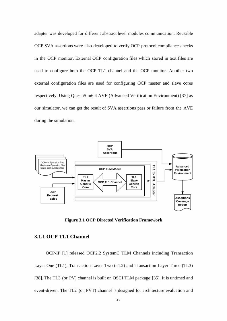
33
adapter was developed for different abstract level modules communication. Reusable
OCP SVA assertions were also developed to verify OCP protocol compliance checks
in the OCP monitor. External OCP configuration files which stored in text files are
used to configure both the OCP TL1 channel and the OCP monitor. Another two
external configuration files are used for configuring OCP master and slave cores
respectively. Using QuestaSim6.4 AVE (Advanced Verification Environment) [37] as
our simulator, we can get the result of SVA assertions pass or failure from the AVE
during the simulation.
Figure 3.1 OCP Directed Verification Framework
3.1.1 OCP TL1 Channel
OCP-IP [1] released OCP2.2 SystemC TLM Channels including Transaction
Layer One (TL1), Transaction Layer Two (TL2) and Transaction Layer Three (TL3)
[38]. The TL3 (or PV) channel is built on OSCI TLM package [35]. It is untimed and
event-driven. The TL2 (or PVT) channel is designed for architecture evaluation and
OCP
SVA
Assertions
OCP
Request
Tables
TL1
Slave
Generic
Core
OCP TL1 Channel
TL1
Master
Generic
Core
Advanced
Verification
Environment
Assertions
Coverage
Report
OCP configuration files
Master configuration files
Slave configuration files
TL
1 to
RT
L A
da
pte
r
OCP TLM Model
34
modeling. It is approximately-timed. The TL1 (or CA) channel is cycle-accurate but
faster than RTL. Even though TL3 and TL2 channels are much more efficient than TL1,
they cannot be our DUV because they hide the protocol details. To develop a reusable
verification framework for both TLM and RTL modules, timing information is
necessary and cannot be ignored. The TL1 channel is the transfer layer channel which
is designed for simulations that are close to the hardware level. We choose the TL1
channel as our DUV because it supports all OCP transfer phases, timing and
configuration parameters of OCP hardware specification. The SVA assertions that are
developed for TL1 channel use to verify OCP protocol and configuration compliance
can be reused for RTL OCP models.
The OCP SystemC TL1 channel uses “request/update” methods for delta cycle
updates of the channel state. It implements the OCP API commands that process
request, data handshake and response OCP transfers. The OCP master and slave
interfaces in the TL1 channel provide port access to all OCP API commands. Moreover,
the TL1 channel implements the monitor interface so that the monitor can be connected
for protocol checking, performance analysis and trace dumping.
The TL1 channel is configured by a C++ STL (Standard Template Library) MAP
object that contains all of the OCP parameter settings. The MAP is constructed by the
key string being the name of the parameter and the value string being the value of the
parameter. An example is shown below:
threads i:8
35
The left side (the key side) of the pair is the OCP parameter name. “threads”
indicates that how many threads are in the OCP channel. The right side (the value side)
are formatted as type_char:value, where type_char can be “i” for an integer or Boolean,
“f” for a floating point value and “s” for a string. A value followed a colon (:) indicates
the value of the OCP parameter. Accordingly, the example means the OCP TL1 model
is configured as an eight-thread OCP channel.
During the elaboration, the OCP TL1 channel loads the OCP parameters from an
external configuration file to build the configuration MAP and sends the corresponding
settings to the OCP generic master core and the OCP generic slave core.
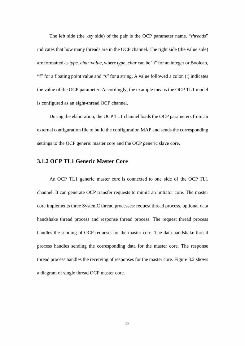
3.1.2 OCP TL1 Generic Master Core
An OCP TL1 generic master core is connected to one side of the OCP TL1
channel. It can generate OCP transfer requests to mimic an initiator core. The master
core implements three SystemC thread processes: request thread process, optional data
handshake thread process and response thread process. The request thread process
handles the sending of OCP requests for the master core. The data handshake thread
process handles sending the corresponding data for the master core. The response
thread process handles the receiving of responses for the master core. Figure 3.2 shows
a diagram of single thread OCP master core.
36
Figure 3.2 OCP TL1 Generic Master Core
As a directed test generator, the master core generates OCP transactions from
few requests tables. The request tables contain OCP commands. The burstlength table
has the lengths for each OCP transaction. The threads table indicates which thread is
used for the corresponding OCP transfer request. The delays between the sending out of
each request are also set in a delays table. An example of request tables is shown as
follows. There are nine predefined OCP transactions in this example. For each table
entry, the master sends the corresponding requests to the corresponding thread then
waits the corresponding time before moving on to the next table entry. At the beginning
of the simulation, the master core gets OCP commands from the first row of the
command table. In this example, there are two OCP simple write commands in the
first transaction. The first element in the thread table indicates that these two
Request
Phase
SCmdAcceptData
Handshake
Phase
SDataAccept
delay
request3
delay
request 2
delay
request 1
……………
Request
Stream
delay
Response
Response
Processing
and
Acceptancedata 4
data 6
data 5
data 4
data 3
data 2
data 1
……………
Data HS
Stream
New
ResponseMRespAccept
OCP Master Core
Single-Threaded OCP
Delays
Table
BurstLength
Table
Threads
Table
Commands
Table
Request
Tables
37
commands should be sent to OCP thread 0. Similarly, the first element of the burst
table gives the burst length of the first transaction according to the number of the
valid OCP commands in the command table. After that, the first entry of the delay
table gives 100 cycles delay for the first command and 3 cycles delay for the second
one. When the first transaction is finished, the master will get the next one according
to the second entry of request tables. During the simulation, the master gets
transactions from request tables in an infinite loop.
// OCP command table
OCPMCmdType Commands[9][4] = {
{OCP_MCMD_WR,OCP_MCMD_WR, OCP_MCMD_IDLE,OCP_MCMD_IDLE},
{OCP_MCMD_WR, OCP_MCMD_WR, OCP_MCMD_WR, OCP_MCMD_IDLE},
{OCP_MCMD_RD,OCP_MCMD_IDLE,OCP_MCMD_IDLEOCP_MCMD_IDLE},
{OCP_MCMD_RD, OCP_MCMD_RD, OCP_MCMD_RD, OCP_MCMD_IDLE},
{OCP_MCMD_RD, OCP_MCMD_RD, OCP_MCMD_RD, OCP_MCMD_IDLE},
{OCP_MCMD_RD, OCP_MCMD_RD, OCP_MCMD_RD, OCP_MCMD_RD},
{OCP_MCMD_RD, OCP_MCMD_RD, OCP_MCMD_IDLE, OCP_MCMD_IDLE},
{OCP_MCMD_WR, OCP_MCMD_WR, OCP_MCMD_WR, OCP_MCMD_IDLE},
{OCP_MCMD_RD, OCP_MCMD_RD, OCP_MCMD_RD, OCP_MCMD_RD}
};
38
//Thread table
unsigned int TestThread[] = {0, 1, 2, 3, 4, 5, 6, 7, 8};
//Burstlength table
int NumTr[] = {2, 3, 1, 3, 3, 4, 2, 3, 4};
// Delay table
int NumWait[NUM_TESTS][4] = {
{100, 3, 0xF, 0xF},
{7, 1, 3, 0xF},
{6, 0xF, 0xF, 0xF},
{10, 2, 1, 0xF},
{7, 1, 3, 0xF},
{6, 1, 1, 1},
{7, 2, 0xF, 0xF},
{8, 2, 1, 0xF},
{7, 2, 2, 2}
};
The master core is generic for different OCP configuration settings. Dashed parts
are optional and can be enabled and disabled by OCP configuration settings. For
example, if the OCP parameter “datahandshake” is set to 1, the master will involve the
39
optional data handshake thread process and send request phase and data handshake
phase separately. Otherwise, it sends OCP transfer request with the data in the request
thread process only.
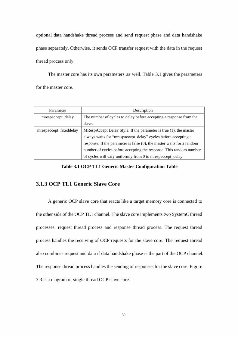
The master core has its own parameters as well. Table 3.1 gives the parameters
for the master core.
Parameter Description
mrespaccept_delay The number of cycles to delay before accepting a response from the
slave.
mrespaccept_fixeddelay MRespAccept Delay Style. If the parameter is true (1), the master
always waits for “mrespaccept_delay” cycles before accepting a
response. If the parameter is false (0), the master waits for a random
number of cycles before accepting the response. This random number
of cycles will vary uniformly from 0 to mrespaccept_delay.
Table 3.1 OCP TL1 Generic Master Configuration Table
3.1.3 OCP TL1 Generic Slave Core
A generic OCP slave core that reacts like a target memory core is connected to
the other side of the OCP TL1 channel. The slave core implements two SystemC thread
processes: request thread process and response thread process. The request thread
process handles the receiving of OCP requests for the slave core. The request thread
also combines request and data if data handshake phase is the part of the OCP channel.
The response thread process handles the sending of responses for the slave core. Figure
3.3 is a diagram of single thread OCP slave core.
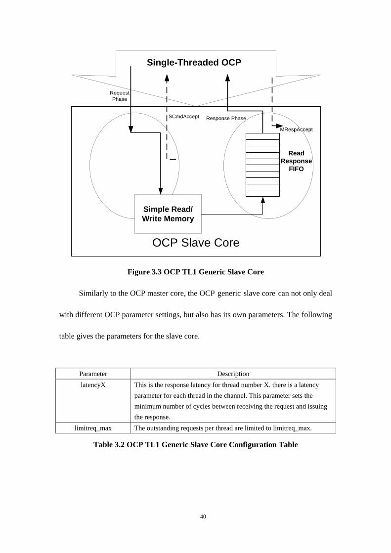
40
Figure 3.3 OCP TL1 Generic Slave Core
Similarly to the OCP master core, the OCP generic slave core can not only deal
with different OCP parameter settings, but also has its own parameters. The following
table gives the parameters for the slave core.
Parameter Description
latencyX This is the response latency for thread number X. there is a latency
parameter for each thread in the channel. This parameter sets the
minimum number of cycles between receiving the request and issuing
the response.
limitreq_max The outstanding requests per thread are limited to limitreq_max.
Table 3.2 OCP TL1 Generic Slave Core Configuration Table
OCP Slave Core
Single-Threaded OCP
Simple Read/
Write Memory
Request
Phase
SCmdAccept
`
Read
Response
FIFO
Response Phase
MRespAccept

41
3.1.4 Reusable OCP Assertions
OCP-IP provides OCP2.2 compliance checks in the specification [16]. For a core
to be considered OCP compliant, it must satisfy all the compliance checks. The
compliance checks include protocol compliance checks and configuration compliance
checks. The compliance checks includes dataflow signals checks, dataflow phase
checks, dataflow burst checks, dataflow transfer checks, sideband checks and so on.
SVA language is chosen to design OCP SVA assertions according to these compliance
checks. All these assertions presented are embedded to a reusable OCP monitors.
The monitor contains a full set of OCP parameters, all OCP signals. During the
simulation, the OCP assertions can be activated or inactivated by the corresponding
OCP parameters. In order to illustrate the approach to verify OCP protocol compliance,
some SVA assertions are present as following.
Dataflow phase check 1.1.2: signal_valid_MCmd_when_reset_inactive [16]
The signal MCmd should never have an X or Z value on the rising edge of the
OCP clock.
property p_signal_valid_MCmd_when_reset_inactive;
@(posedge ocpif.sv_clk) disable iff (!ocpif.MReset_n)
!$isunknown(ocpif.MCmd);
endproperty
42
Dataflow phase check 1.2.3: request_hold_MCmd [16]
Once a request phase has begun, the signal MCmd may not change their value
until the OCP Slave has accepted the request. This check is active only if the OCP
parameter cmdaccept, is set to 1. The request phase begins when the master drives
MCmd to a value other than Idle and ends when SCmdAccept is sampled asserted (true)
by the rising edge of the OCP clock. The SVA assertion for this check shows below:
property p_request_hold_MCmd;
@(posedge ocpif.sv_clk) disable iff(!ocpif.MReset_n||!ocpif.SReset_n)
first_match (ocpif.MCmd!=OCP_MCMD_IDLE&&
!ocpif.SCmdAccept && ocpif.ocpParams.cmdaccept)
|=>$stable(ocpif.MCmd) throughout
(##[0:$]$rose(ocpif.SCmdAccept));
endproperty
Dataflow burst check 1.3.7: burst_sequence_MAddr_INCR [16]
Within an INCR burst, the address increases for each new master request by the
OCP word size. Because an INCR burst can be a precise burst or an imprecise burst.
Obviously, we cannot translate this check into one SVA assertion. We have to separate
the check into individual SVA assertions for all possible bursts.
There are two types of OCP precise burst, MRMD burst and SRMD burst. For
SRMD burst, only the first request will be sent out, so this check makes nonsense for
SRMD burst. For MRMD burst, although the burst length is constant, different MRMD
43
bursts can have different lengths. However, SVA repetition operator must have a fixed
value as the number of times the expression should match, so it‟s impossible to design
one assertion for different MRMD bursts with different lengths. This problem was
solved by defining a macro, putting the macro inside the repetition operator of the SVA
assertion as a constant. Even though the assertion can only check fixed length MRMD
burst in one simulation, different length bursts can be checked in different simulations
by changing the macro value then rebuilding the monitor module before running
another simulation. The SVA code shows below:
property p_burst_sequence_MAddr_INCR_precise;
logic[2:0] old_cmd;
@(posedge ocpif.sv_clk) disable iff(!ocpif.MReset_n)
if(ocpif.ocpParams.burstlength&& ocpif.ocpParams.addr &&
ocpif.ocpParams.burstseq_incr_enable&&
ocpif.ocpParams.burstseq)
(first_match(ocpif.MCmd!=OCP_MCMD_IDLE&&
ocpif.MBurstLength==`BURST_LENGTH &&
ocpif.MBurstSeq==OCP_MBURSTSEQ_INCR &&
((ocpif.MBurstPrecise&&ocpif.ocpParams.burstprecise)
|| !ocpif.ocpParams.burstprecise)&&
((!ocpif.MBurstSingleReq&&ocpif.ocpParams.burstsinglereq)
|| !ocpif.ocpParams.burstsinglereq)),
44
old_cmd = ocpif.MCmd)
|=>(((ocpif.MAddr-$past(ocpif.MAddr))==ocpif.ocpParams.data_wdt
h/8) && ocpif.MCmd==old_cmd) [->`BURST_LENGTH-1];
endproperty
For imprecise burst, the way to decide the beginning and the end of a burst are
different from precise burst. The beginning of an imprecise burst is the first request
phase with MBurstLength greater than 1. The end of an imprecise burst is the request
phase with MBurstLength equal to 1. So the SVA code shows below:
property p_burst_sequence_MAddr_INCR_imprecise;
logic[2:0] old_cmd;
@(posedge ocpif.sv_clk) disable iff(!ocpif.MReset_n)
if(ocpif.ocpParams.burstprecise && ocpif.ocpParams.burstlength &&
ocpif.ocpParams.addr && ocpif.ocpParams.burstseq_incr_enable &&
ocpif.ocpParams.burstseq)
first_match(ocpif.MCmd!=OCP_MCMD_IDLE&&
ocpif.MBurstLength>1 &&
ocpif.MBurstSeq==OCP_MBURSTSEQ_INCR &&
!ocpif.MBurstPrecise),
old_cmd = ocpif.MCmd
|=> ((ocpif.MAddr-$past(ocpif.MAddr)==ocpif.ocpParams.data_wdth/8)
&&ocpif.MCmd==old_cmd&&ocpif.MBurstLength>1)[->0:$] ##[1:$]
45
(ocpif.MAddr-$past(ocpif.MAddr)==ocpif.ocpParams.data_wdth/8) &&
ocpif.MCmd==old_cmd && ocpif.MBurstLength==1;
endproperty
The monitor includes not only the protocol compliance checks as above, but also
the configuration compliance checks which involve enable relationships of OCP
parameters. These configuration checks “param1_enable_param2” implies that param1
is somehow enabled by param2.
Request group check 2.1.7: req_cfg_sdata_enable_resp [16]
The parameter “sdata” can only be enabled if “resp” is enabled.
property P_req_cfg_sdata_enable_resp;
sdata==1 |-> resp==1;
endproperty
The OCP reusable monitor can load OCP parameters from the configuration text
files before the simulation just like the OCP TL1 channel does. All the SVA assertions
are activated only when the corresponding OCP parameters are enabled.
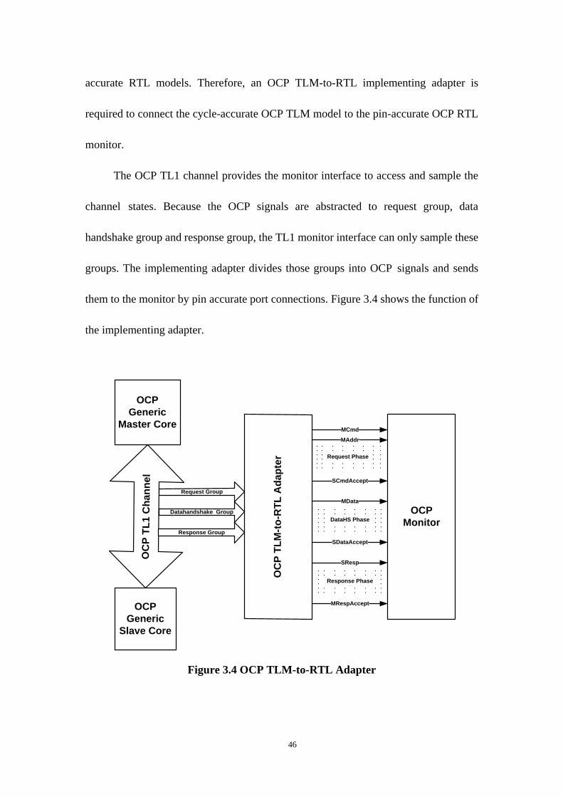
3.1.5 OCP TLM-to-RTL Adapter
Even though OCP TL1 channel is cycle accurate, it is still high level abstract
model without OCP signals in the Channel. The master and slave communicated by
functional calls. On the other hand, our reusable OCP SVA assertions are developed
based on OCP protocol compliance checks. All these checks are represented by OCP
signals. The OCP monitor that contains the reusable SVA assertions should be pin
46
accurate RTL models. Therefore, an OCP TLM-to-RTL implementing adapter is
required to connect the cycle-accurate OCP TLM model to the pin-accurate OCP RTL
monitor.
The OCP TL1 channel provides the monitor interface to access and sample the
channel states. Because the OCP signals are abstracted to request group, data
handshake group and response group, the TL1 monitor interface can only sample these
groups. The implementing adapter divides those groups into OCP signals and sends
them to the monitor by pin accurate port connections. Figure 3.4 shows the function of
the implementing adapter.
Figure 3.4 OCP TLM-to-RTL Adapter
OCP
Generic
Master Core
Request Group
OC
P T
L1
Ch
an
ne
l
OCP
Generic
Slave Core
OC
P T
LM
-to
-RT
L A
da
pte
r
OCP
Monitor
Datahandshake Group
Response Group
MCmd
MAddr
SCmdAccept
MData
SDataAccept
SResp
MRespAccept
Request Phase
DataHS Phase
Response Phase
47
First of all, the implementing adapter samples OCP TL1 request group, OCP TL1
data handshake group and OCP TL1 response group by the positive edge of each clock
cycle. Then those groups are divided into OCP signals. After that, a set of SystemC
ports (sc_out) for each OCP signal were defined for communication with the monitor.
Finally, the powerful QuestaSim6.4 AVE was employed to connect the SystemC model
(OCP TL1 channel) and the SystemVerilog model (OCP SVA monitor) because it
supports mix-language design and verification simulation. Following the QuestaSim
user‟s manual guidelines [37], the SystemC DUV can be instantiated in the
SystemVerilog monitor and communication with the monitor.
3.2 OCP Verification Framework with SCV Generator
The previous OCP verification framework utilized directed test scheme because
the generic OCP master core gets test scenarios from request tables. As SoC designs
grow larger, it becomes more difficult to generate a complete set of directed stimuli to
cover their full functionality. A solution to overcome the weakness of directed test is
using automatic constraint-random test (CRT). In this these, we employ SystemC
verification library (SCV) as a traditional pure random number generator to produce
random OCP transactions for our OCP models.
Figure 3.5 depicts the verification methodology. Instead of using directed OCP
request tables, a SCV random OCP transaction generator is developed to target our
OCP models. Because OCP has the high configurability and flexibility, the SCV
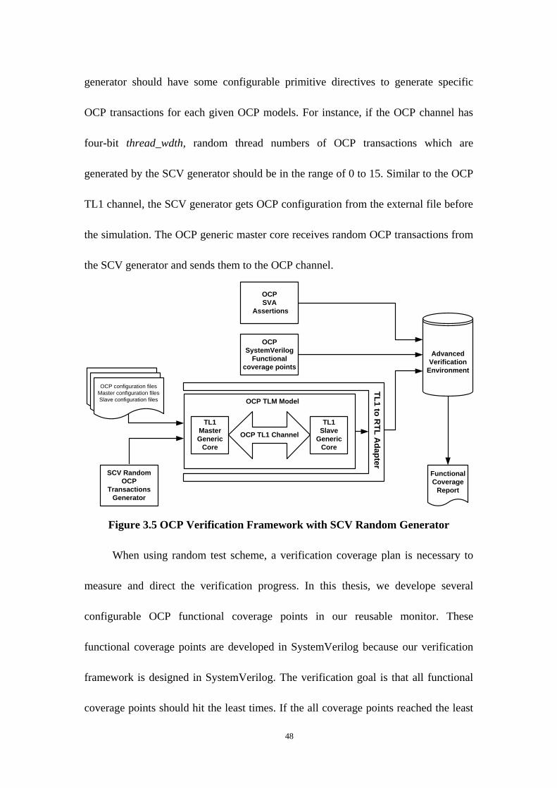
48
generator should have some configurable primitive directives to generate specific
OCP transactions for each given OCP models. For instance, if the OCP channel has
four-bit thread_wdth, random thread numbers of OCP transactions which are
generated by the SCV generator should be in the range of 0 to 15. Similar to the OCP
TL1 channel, the SCV generator gets OCP configuration from the external file before
the simulation. The OCP generic master core receives random OCP transactions from
the SCV generator and sends them to the OCP channel.
Figure 3.5 OCP Verification Framework with SCV Random Generator
When using random test scheme, a verification coverage plan is necessary to
measure and direct the verification progress. In this thesis, we develope several
configurable OCP functional coverage points in our reusable monitor. These
functional coverage points are developed in SystemVerilog because our verification
framework is designed in SystemVerilog. The verification goal is that all functional
coverage points should hit the least times. If the all coverage points reached the least
OCP
SystemVerilog
Functional
coverage points
SCV Random
OCP
Transactions
Generator
TL1
Slave
Generic
Core
OCP TL1 Channel
TL1
Master
Generic
Core
Advanced
Verification
Environment
Functional
Coverage
Report
OCP configuration files
Master configuration files
Slave configuration files
OCP
SVA
Assertions
TL
1 to
RT
L A
da
pte
r
OCP TLM Model
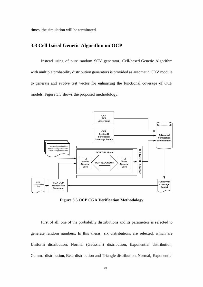
49
times, the simulation will be terminated.
3.3 Cell-based Genetic Algorithm on OCP
Instead using of pure random SCV generator, Cell-based Genetic Algorithm
with multiple probability distribution generators is provided as automatic CDV module
to generate and evolve test vector for enhancing the functional coverage of OCP
models. Figure 3.5 shows the proposed methodology.
Figure 3.5 OCP CGA Verification Methodology
First of all, one of the probability distributions and its parameters is selected to
generate random numbers. In this thesis, six distributions are selected, which are
Uniform distribution, Normal (Gaussian) distribution, Exponential distribution,
Gamma distribution, Beta distribution and Triangle distribution. Normal, Exponential
OCP
SystemC
Functional
Coverage Points
CGA OCP
Transaction
Generator
Functional
Coverage
Report
OCP configuration files
Master configuration files
Slave configuration files
OCP
SVA
Assertions
CGA
Configuration
File
Advanced
Verification
Environment
TL1
Slave
Generic
Core
OCP TL1 Channel
TL1
Master
Generic
Core
TL
1 to
RT
L A
da
pte
r
OCP TLM Model
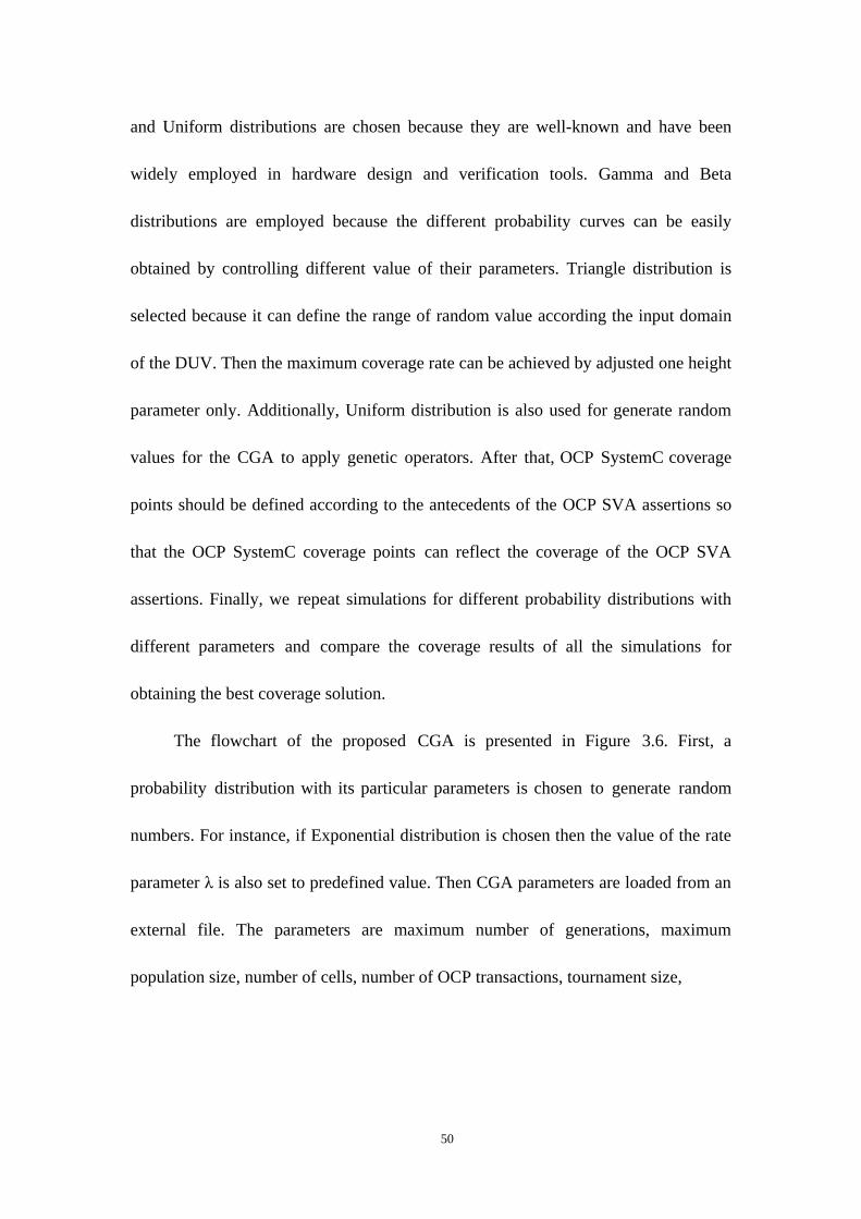
50
and Uniform distributions are chosen because they are well-known and have been
widely employed in hardware design and verification tools. Gamma and Beta
distributions are employed because the different probability curves can be easily
obtained by controlling different value of their parameters. Triangle distribution is
selected because it can define the range of random value according the input domain
of the DUV. Then the maximum coverage rate can be achieved by adjusted one height
parameter only. Additionally, Uniform distribution is also used for generate random
values for the CGA to apply genetic operators. After that, OCP SystemC coverage
points should be defined according to the antecedents of the OCP SVA assertions so
that the OCP SystemC coverage points can reflect the coverage of the OCP SVA
assertions. Finally, we repeat simulations for different probability distributions with
different parameters and compare the coverage results of all the simulations for
obtaining the best coverage solution.
The flowchart of the proposed CGA is presented in Figure 3.6. First, a
probability distribution with its particular parameters is chosen to generate random
numbers. For instance, if Exponential distribution is chosen then the value of the rate
parameter λ is also set to predefined value. Then CGA parameters are loaded from an
external file. The parameters are maximum number of generations, maximum
population size, number of cells, number of OCP transactions, tournament size,
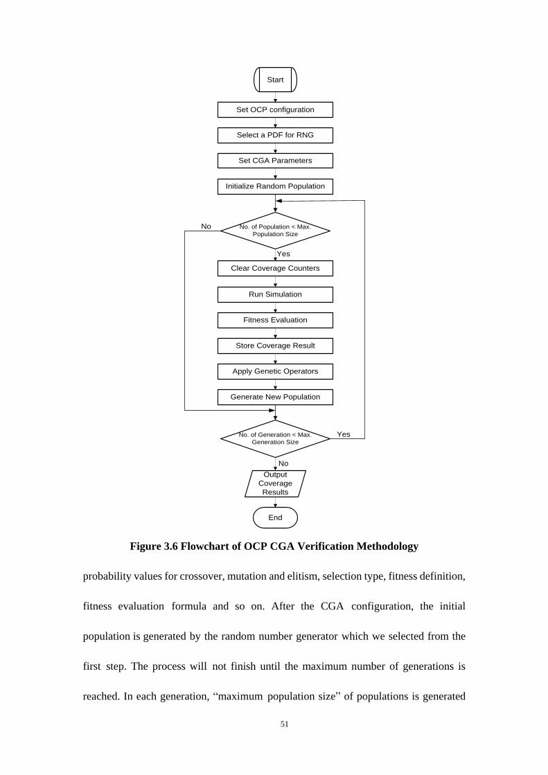
51
Figure 3.6 Flowchart of OCP CGA Verification Methodology
probability values for crossover, mutation and elitism, selection type, fitness definition,
fitness evaluation formula and so on. After the CGA configuration, the initial
population is generated by the random number generator which we selected from the
first step. The process will not finish until the maximum number of generations is
reached. In each generation, “maximum population size” of populations is generated
End
Start
Select a PDF for RNG
Set CGA Parameters
Initialize Random Population
Clear Coverage Counters
Run Simulation
Fitness Evaluation
Store Coverage Result
Apply Genetic Operators
Generate New Population
Output
Coverage
Results
No. of Population < Max.
Population Size
No. of Generation < Max.
Generation Size
Yes
Yes
No
No
Set OCP configuration
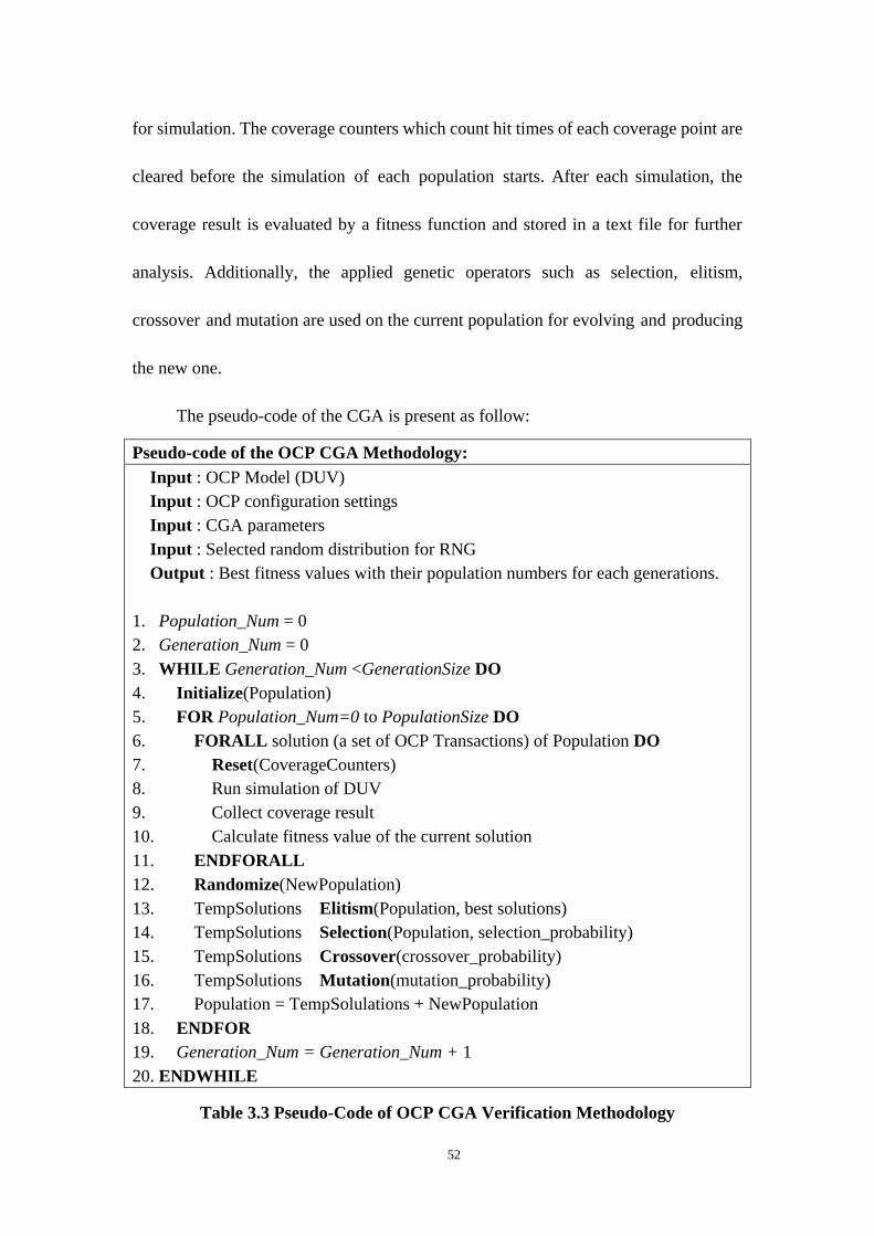
52
for simulation. The coverage counters which count hit times of each coverage point are
cleared before the simulation of each population starts. After each simulation, the
coverage result is evaluated by a fitness function and stored in a text file for further
analysis. Additionally, the applied genetic operators such as selection, elitism,
crossover and mutation are used on the current population for evolving and producing
the new one.
The pseudo-code of the CGA is present as follow:
Pseudo-code of the OCP CGA Methodology:
Input : OCP Model (DUV)
Input : OCP configuration settings
Input : CGA parameters
Input : Selected random distribution for RNG
Output : Best fitness values with their population numbers for each generations.
1. Population_Num = 0
2. Generation_Num = 0
3. WHILE Generation_Num <GenerationSize DO
4. Initialize(Population)
5. FOR Population_Num=0 to PopulationSize DO
6. FORALL solution (a set of OCP Transactions) of Population DO
7. Reset(CoverageCounters)
8. Run simulation of DUV
9. Collect coverage result
10. Calculate fitness value of the current solution
11. ENDFORALL
12. Randomize(NewPopulation)
13. TempSolutions Elitism(Population, best solutions)
14. TempSolutions Selection(Population, selection_probability)
15. TempSolutions Crossover(crossover_probability)
16. TempSolutions Mutation(mutation_probability)
17. Population = TempSolulations + NewPopulation
18. ENDFOR
19. Generation_Num = Generation_Num + 1
20. ENDWHILE
Table 3.3 Pseudo-Code of OCP CGA Verification Methodology
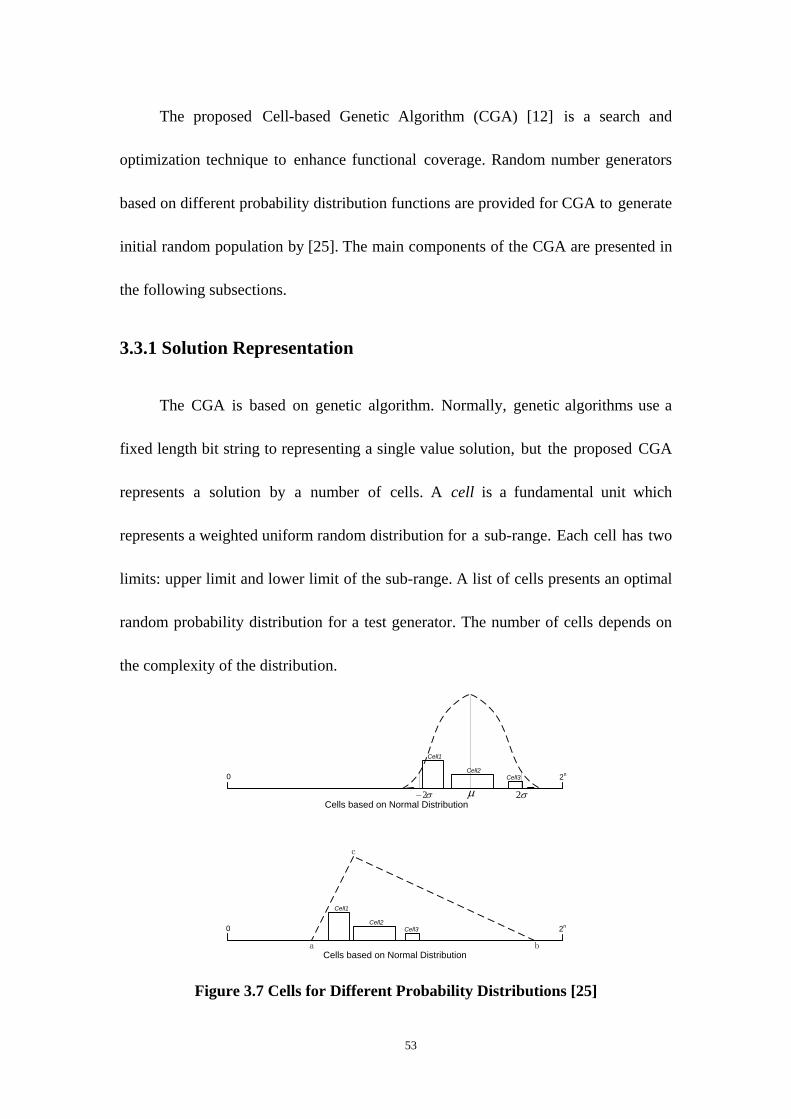
53
The proposed Cell-based Genetic Algorithm (CGA) [12] is a search and
optimization technique to enhance functional coverage. Random number generators
based on different probability distribution functions are provided for CGA to generate
initial random population by [25]. The main components of the CGA are presented in
the following subsections.
3.3.1 Solution Representation
The CGA is based on genetic algorithm. Normally, genetic algorithms use a
fixed length bit string to representing a single value solution, but the proposed CGA
represents a solution by a number of cells. A cell is a fundamental unit which
represents a weighted uniform random distribution for a sub-range. Each cell has two
limits: upper limit and lower limit of the sub-range. A list of cells presents an optimal
random probability distribution for a test generator. The number of cells depends on
the complexity of the distribution.
Figure 3.7 Cells for Different Probability Distributions [25]
2
2n 0
Cell1
Cell2Cell3
2n0
Cell1
Cell2Cell3
a b
c
Cells based on Normal Distribution
Cells based on Normal Distribution
2
54
The solution of an OCP model in the CGA depends on the configuration of the
model and the verification plan (functional coverage points) of the model. For
instance, an OCP TL1 model only supports OCP simple read command
(OCP_MCMD_RD) and simple write command (OCP_MCMD_WR) and the
verification plan is that both OCP_MCMD_RD and OCP_MCMD_WR should be
presented on the OCP channel. Then, the solution of the CGA can be represented
by only 1 bit. The value of 0 represents OCP_MCMD_RD and the value of 1
represents OCP_MCMD_WR.
If the solution of an OCP model is represented by n bits, the parameters of cells
are generated within the range of 0 to -1 by a random number generator. The initial
population of the CGA is comprised of a number of cells. The total number of cells is
configured by an external CGA configuration file which can be predefined by the user
before simulation. Each cell has three parameters, which are lower limit, high limit and
weight of the uniform distribution. The random generation of these parameters is
based on the selected probability distribution. Figure 3.7 shows two groups of cells
which are generated based on a Normal distribution and a Triangle distribution
respectively. Random numbers in each cell are stimuli of the OCP model. Coverage
information is collected for each cell for evaluation and evolution during the
simulation.
A group of cells which represents a probability distribution is called
Chromosome. Each chromosome is considered as a stimuli generator. Several
55
parameters in each chromosome, such as the maximum valid range and the total
weight of all cells, are provided for the evolution process. Normally, many test
generators are needed to drive the DUV. A collection of Chromosomes constitutes a
Genome which represents a whole solution. A genome also has many parameters for
the evolution process such as the complexity of a chromosome which is the total
number of cells in it, the mutation probability of a cell and the crossover
probability of a chromosome and so on. These parameters are also configured
from an external CGA configuration file are constant during the process.
3.3.2 Random Number Generators
A Random Number Generator (RNG) is computational program which is
designed to generate a sequence of stimuli for the DUV without any pattern. RNGs are
widely used in simulation-based verification and evolution processes. Normally, a
RNG with uniform distribution between 0 and 1 is required to generate any specific
probability distribution. In the CGA, a Pseudo-Random Number Generator (PRNG)
algorithm called Mersenne Twister (MT) [40] is utilized to generate good quality
random numbers uniformly distributed between 0 and 1. Normal distribution,
Exponential distribution, Gamma distribution, Beat distribution and Triangle
distribution random number generators are provided based on the MT algorithm to
generate stimuli for OCP model.
There are several techniques can be used for generating random numbers from
different probability distributions such as inverse Cumulative Distribution Function
56
(CDF) technique, Acceptance-Rejection technique [41]. The inverse CDF technique
substitutes a random uniform number between 0 and 1 in the CDF of the selected
probability distribution function (PDF) for generating distributed random numbers. The
acceptance-rejection technique samples two values. One is the PDF f(x), where x is a
random number. The other on is y from U(0,1). If f(x)>y, the value of x is accepted. If
not, reject the value x and repeat sampling. Some other methods are used for specific
probability distributions such as Box-Muller and Polar technique for normal
distribution [42].
In the proposed methodology, different techniques are applied to implement five
different probability distributions based on the work of [25]. Inverse CDF technique is
used for implementing exponential and triangle distributions [41].
Acceptance-rejection technique is used for formulating Gamma and Beta distributions
[43]. And Box-Muller method is chosen for Normal distribution [42]. Additionally,
uniformly distribution random numbers generated by MT are provided for all these
technique algorithms.
3.3.3 Initialization
The first step of a Genetic Algorithm is generating an initial random population.
The CGA utilized two optional initialization schemes: fixed period random
initialization and random period random initialization. Figure 3.8 illustrates a five-cell
initialization by these two schemes respectively.
In fixed period random initialization, the input valid range [0, ] is divided
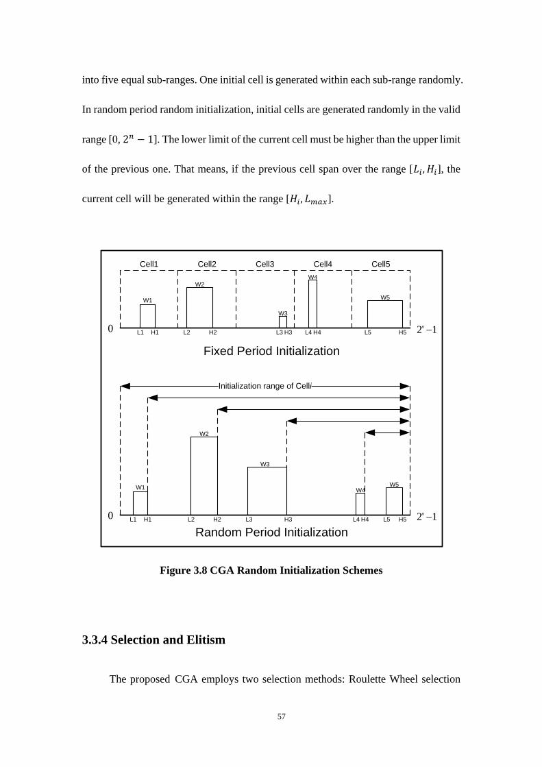
57
into five equal sub-ranges. One initial cell is generated within each sub-range randomly.
In random period random initialization, initial cells are generated randomly in the valid
range [0, ]. The lower limit of the current cell must be higher than the upper limit
of the previous one. That means, if the previous cell span over the range [ ], the
current cell will be generated within the range [ ].
Figure 3.8 CGA Random Initialization Schemes
3.3.4 Selection and Elitism
The proposed CGA employs two selection methods: Roulette Wheel selection
Cell1 Cell2 Cell3 Cell4 Cell5
L1 H1
W1
L2 H2
W2
L3 H3
W3
L4 H4
W4
L5 H5
W5
12 n0
L1 H1
W1
L2 H2
W2
L3 H3
W3
L4 H4
W4
L5 H5
W5
12 n0
Initialization range of Celli
Fixed Period Initialization
Random Period Initialization

58
and Tournament selection [26]. This option is in the CGA configuration file and users
can choose one of them before the simulation. The elitism operator is also applied at
the same time to keep the fittest individuals in the next generation.
3.3.5 Crossover
Crossover operator is useful to preserve and forwards good features of exist
individuals to the next generation. In the CGA, crossover operators are applied to
chromosomes with a probability parameter . A uniformly random number
is generated for each chromosome to compare with . If is less than ,
then crossover operator will be executed to the chromosome. Otherwise, the
chromosome will be copied to the new generation directly.
Two kinds of crossover operators are provided in the CGA, which are single
point crossover and inter-cell crossover. Single point crossover is the typical crossover
that exchanges cells between two chromosomes. Inter-cell crossover operator merges
two chromosomes by union ( ) or intersection (
) rather than exchange parts of them. Which kind of crossover operator is
selected depends on the predefined weights and . Similar to the
previous scheme, a uniformly random number is
generated. Single point crossover operator is chosen if . Inter-cell
crossover is selected if .
59
3.3.6 Mutation
The purpose of mutation operators is introducing new features to new generators.
In the CGA, mutation operators are applied to chromosomes with a probability for
each cell. Many mutation operators are provided to mutate the low limit, high limit and
the weight of a cell. Similar to crossover operator, the predefined weights of the
mutation operators are used to decide which one will be applied. When a cell is selected
for mutation, one of the following operators should be applied:
Insert or delete a cell
Shift or adjust a cell
Change the weight of a cell
3.3.7 Fitness Evaluation
A sequence of cells is considered as a potential solution of the CGA to direct a
random number generator to improve the coverage rate of a set of functional coverage
points. The fitness value which is calculated by an evaluation function represents the
quality of the solution. A greater fitness value that a solution has, a greater coverage
rate the solution can reach.
Different evaluation functions can be employed in the CGA. The average
coverage rate is the most common strategy. However, it is not a good evaluation
function to discriminate potential solutions when there are many coverage points to be
considered simultaneously. Assume we have two potential solutions. One solution
60
with high average rate is obtained by most of 100% coverage points and few totally
inactivated coverage point. The other solution with a low average coverage rate is
comprised of all the coverage points having a low but non-zero coverage rate.
Apparently, the second solution is better than the first one because all the coverage
points are activated. But the average coverage rates show the opposite result.
Consequently, two evaluation functions are defined in the CGA. One function is
Four-Stage Evaluation, the other one is Mean-Weighted Standard Deviation
Difference Evaluation.
Four-stage evaluation method ensures that the evaluation process will activate all
coverage points before tending to maximize the average coverage rate. The main steps
of the four-stage method are presented as follows:
Find a solution that activates all the coverage points at least one time.
Push the solution towards activating all the coverage points according to a
predefined coverage rate threshold CovRate1.
Push the solution towards activating all the coverage points according to a
predefined coverage rate threshold CovRate2 which is higher than
CovRate1.
After achieving the three steps, the average coverage rate of all the
coverage points is applied for continuous evolution.
The other evaluation function is Mean-Weighted Standard Deviation Difference
Evaluation. Its equation is presented below:
61
(3.1)
Where and
(3.2)
(3.3)
According to the equation, better fitness value can be achieved by increasing the
average coverage ( ) and decreasing the standard deviation coverage ( ).
The constant parameter k is used to adjust the effectiveness of the standard deviation.
We may not obtain an effective solution if the value of k is too small. While a large
value of k may also obstruct the way of evolving an effective solution.
3.3.8 Termination Criterion
The termination criterion of the CGA decides whether the evolution process
terminates or continues generating a new potential solution. If the process achieves 100%
or other predefined acceptable values of coverage rate for all the coverage points, the
process will terminate. Otherwise, the CGA runs until the maximum number of
generations is reached and reports the best solution in all potential solutions regardless
of the fitness value. In this thesis, the CGA process will be terminated only when the
maximum number of generations is reached.
3.3.9 OCP SystemC Functional Coverage Points
Our CGA is built in C++ language and our previous OCP functional coverage

62
points in the verification environment are built in SystemVerilog. The CGA module
must keep obtaining coverage information and using the information to evolve
populations during the simulation, but it‟s not efficient to share coverage information
between two different languages. Therefore, we design functional coverage points in
SystemC instead of SystemVerilog in our CGA methodology.
Chapter4
Implementation Result
In this chapter, directed tests are used for five different OCP TL1 models to
activate our protocol compliance assertions and debug both OCP models and
assertions. Then the proposed CGA methodology is utilized to generate random OCP
transactions and evolve transactions to enhance functional coverage of the OCP TL1
MRMD model. MRMD configuration is chosen because it integrates a lot of OCP
configurable features such as data handshake, multi-thread, precise burst and so on. The
SCV random OCP transaction generator is also implemented as pure random stimulus
generator on the MRMD model to compare with the CGA methodology.
4.1 Directed Tests
In this section, an OCP TL1 generic master core gets OCP transactions from
directed test request tables and sends them to an OCP TL1 generic slave core through
the OCP TL1 channel. Five external OCP configuration files are provides to configure
the OCP models. A monitor with reusable OCP SVA assertions is connected to the
OCP TL1 channel for protocol compliance checking. The experimental assertion
coverage results of different OCP models are shown and discussed as well.
64
4.1.1 Five OCP TL1 models
The OCP TL1 generic master core, slave core and channel can be configured to
specific OCP entities by external configuration files. Five OCP configuration settings
were created to demonstrate different OCP features, which are basic configuration,
data handshake configuration, multithreads configuration, MRMD burst configuration
and SRMD configuration. Since we are applying functional verification, some OCP
parameters such as “addr_wdth” and “data_wdth” are not important to demonstrate
OCP features, common values for these parameters are chosen to complete
configuration settings. Basic configuration only supports basic OCP features. The
master core can only send a single request command in each OCP transaction. In data
handshake configuration, the OCP TL1 channel includes data handshake phase so the
OCP master can send request and its data separately. Multithread configuration
enhances the data handshake configuration by adding multiple independent OCP
threads. Different OCP transactions can be transferred in different threads
independently. MRMD and SRMD configuration settings make the TL1 channel
support OCP burst transactions. Moreover, SRMD can accomplish an OCP burst
transaction by a single request. Because these five configuration settings cover main
OCP extension features, almost all of the OCP SVA assertions in the monitor can be
activated and exercised.
Table 4.1 summarizes the basic OCP configuration setting. The basic
configuration sets OCP TL1 channel with only basic OCP features. “addr_wdth=16”

65
and “data_wdth=32” indicate the channel has 16 bits address bus and 32 bits data bus.
“cmdaccept=1” configures the signal SCmdAccept is the part of the OCP channel. A
value of 1 indicates that the OCP slave core has already accepted the current request
from the master core. “write_enable=1” and “read_enable=1” indicate that the
channel only supports basic read and basic write OCP commands. “endian=1”
indicates the channel is little endian, which means lower addresses are associated with
lower numbered data bits (byte lanes).
Parameter Value Parameter Value Parameter Value
addr_wdth 16 broadcast_enable 0 mdata 1
data_wdth 32 rdlwrc_enable 0 sdata 1
threads 1 readex_enable 0 addrspace 0
datahandshake 0 burst_aligned 0 burstprecise 0
cmdaccept 1 force_aligned 0 byteen 0
dataaccept 0 write_enable 1 connid 0
sthreadbusy 0 read_enable 1 reqinfo 0
sthreadbusy_exact 0 writenonpost_enable 0 mdatainfo 0
respaccept 0 writeresp_enable 0 respinfo 0
mthreadbusy 0 addr 1 sdatainfo 0
mthreadbusy_exact 0 resp 1 endian 1
Table 4.1 Basic OCP Configuration
The following tables with highlight parameters show how to configure an OCP
TL1 channel with different OCP extension features.
In Table 4.2, “datahandshake” and “dataaccept” are toggled to 1, which added
data handshake phase with the signal SDataAccept to the OCP TL1 channel. So the
master core can sent the request and data separately during write transfer request. The
value of 1 on the SDataAccept indicates that the slave core accepts the pipelined write
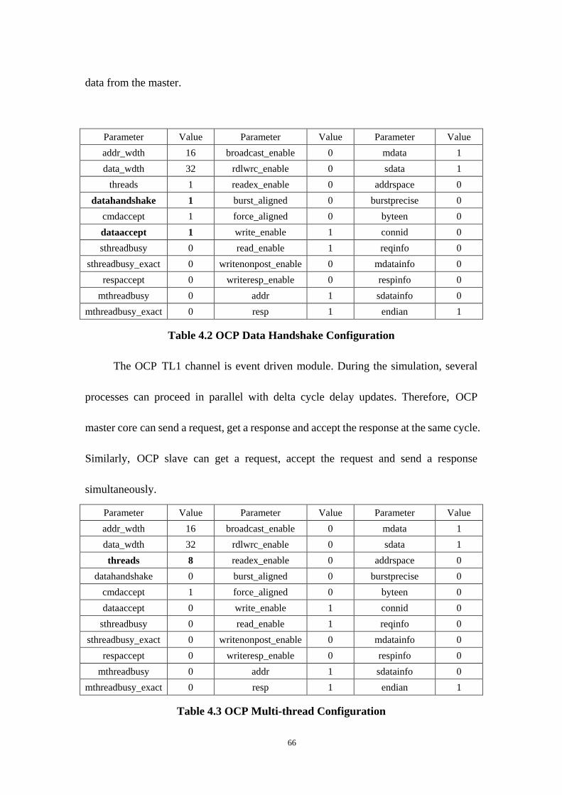
66
data from the master.
Parameter Value Parameter Value Parameter Value
addr_wdth 16 broadcast_enable 0 mdata 1
data_wdth 32 rdlwrc_enable 0 sdata 1
threads 1 readex_enable 0 addrspace 0
datahandshake 1 burst_aligned 0 burstprecise 0
cmdaccept 1 force_aligned 0 byteen 0
dataaccept 1 write_enable 1 connid 0
sthreadbusy 0 read_enable 1 reqinfo 0
sthreadbusy_exact 0 writenonpost_enable 0 mdatainfo 0
respaccept 0 writeresp_enable 0 respinfo 0
mthreadbusy 0 addr 1 sdatainfo 0
mthreadbusy_exact 0 resp 1 endian 1
Table 4.2 OCP Data Handshake Configuration
The OCP TL1 channel is event driven module. During the simulation, several
processes can proceed in parallel with delta cycle delay updates. Therefore, OCP
master core can send a request, get a response and accept the response at the same cycle.
Similarly, OCP slave can get a request, accept the request and send a response
simultaneously.
Parameter Value Parameter Value Parameter Value
addr_wdth 16 broadcast_enable 0 mdata 1
data_wdth 32 rdlwrc_enable 0 sdata 1
threads 8 readex_enable 0 addrspace 0
datahandshake 0 burst_aligned 0 burstprecise 0
cmdaccept 1 force_aligned 0 byteen 0
dataaccept 0 write_enable 1 connid 0
sthreadbusy 0 read_enable 1 reqinfo 0
sthreadbusy_exact 0 writenonpost_enable 0 mdatainfo 0
respaccept 0 writeresp_enable 0 respinfo 0
mthreadbusy 0 addr 1 sdatainfo 0
mthreadbusy_exact 0 resp 1 endian 1
Table 4.3 OCP Multi-thread Configuration
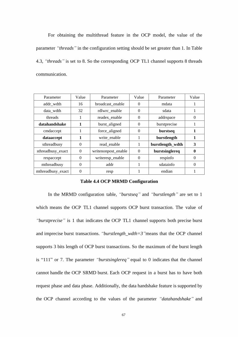
67
For obtaining the multithread feature in the OCP model, the value of the
parameter “threads” in the configuration setting should be set greater than 1. In Table
4.3, “threads” is set to 8. So the corresponding OCP TL1 channel supports 8 threads
communication.
Parameter Value Parameter Value Parameter Value
addr_wdth 16 broadcast_enable 0 mdata 1
data_wdth 32 rdlwrc_enable 0 sdata 1
threads 1 readex_enable 0 addrspace 0
datahandshake 1 burst_aligned 0 burstprecise 1
cmdaccept 1 force_aligned 0 burstseq 1
dataaccept 1 write_enable 1 burstlength 1
sthreadbusy 0 read_enable 1 burstlength_wdth 3
sthreadbusy_exact 0 writenonpost_enable 0 burstsinglereq 0
respaccept 0 writeresp_enable 0 respinfo 0
mthreadbusy 0 addr 1 sdatainfo 0
mthreadbusy_exact 0 resp 1 endian 1
Table 4.4 OCP MRMD Configuration
In the MRMD configuration table, “burstseq” and “burstlength” are set to 1
which means the OCP TL1 channel supports OCP burst transaction. The value of
“burstprecise” is 1 that indicates the OCP TL1 channel supports both precise burst
and imprecise burst transactions. “burstlength_wdth=3”means that the OCP channel
supports 3 bits length of OCP burst transactions. So the maximum of the burst length
is “111” or 7. The parameter “burstsinglereq” equal to 0 indicates that the channel
cannot handle the OCP SRMD burst. Each OCP request in a burst has to have both
request phase and data phase. Additionally, the data handshake feature is supported by
the OCP channel according to the values of the parameter “datahandshake” and
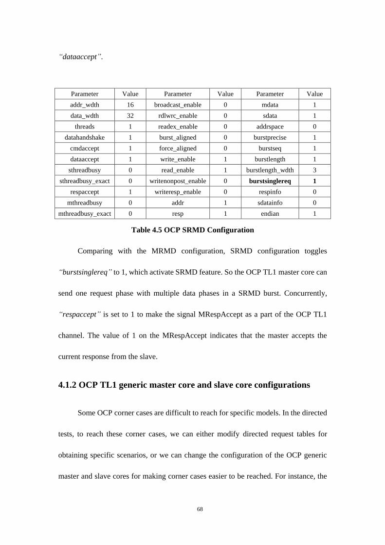
68
“dataaccept”.
Parameter Value Parameter Value Parameter Value
addr_wdth 16 broadcast_enable 0 mdata 1
data_wdth 32 rdlwrc_enable 0 sdata 1
threads 1 readex_enable 0 addrspace 0
datahandshake 1 burst_aligned 0 burstprecise 1
cmdaccept 1 force_aligned 0 burstseq 1
dataaccept 1 write_enable 1 burstlength 1
sthreadbusy 0 read_enable 1 burstlength_wdth 3
sthreadbusy_exact 0 writenonpost_enable 0 burstsinglereq 1
respaccept 1 writeresp_enable 0 respinfo 0
mthreadbusy 0 addr 1 sdatainfo 0
mthreadbusy_exact 0 resp 1 endian 1
Table 4.5 OCP SRMD Configuration
Comparing with the MRMD configuration, SRMD configuration toggles
“burstsinglereq” to 1, which activate SRMD feature. So the OCP TL1 master core can
send one request phase with multiple data phases in a SRMD burst. Concurrently,
“respaccept” is set to 1 to make the signal MRespAccept as a part of the OCP TL1
channel. The value of 1 on the MRespAccept indicates that the master accepts the
current response from the slave.
4.1.2 OCP TL1 generic master core and slave core configurations
Some OCP corner cases are difficult to reach for specific models. In the directed
tests, to reach these corner cases, we can either modify directed request tables for
obtaining specific scenarios, or we can change the configuration of the OCP generic
master and slave cores for making corner cases easier to be reached. For instance, the
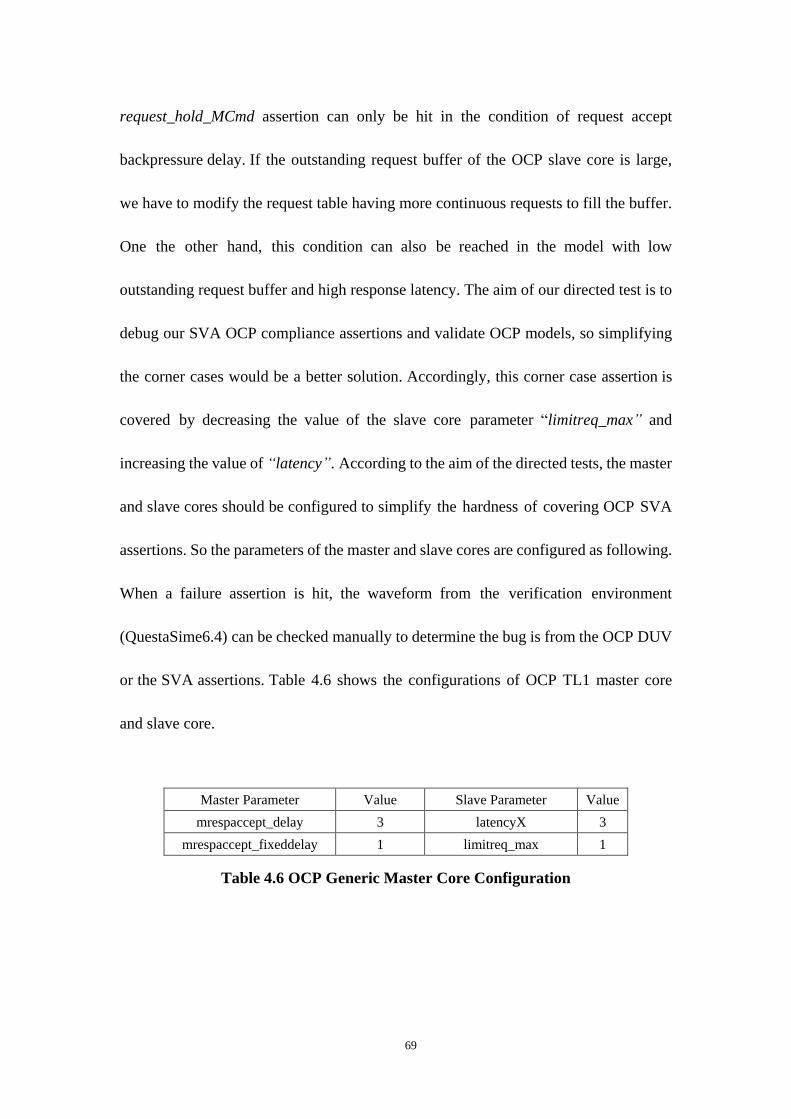
69
request_hold_MCmd assertion can only be hit in the condition of request accept
backpressure delay. If the outstanding request buffer of the OCP slave core is large,
we have to modify the request table having more continuous requests to fill the buffer.
One the other hand, this condition can also be reached in the model with low
outstanding request buffer and high response latency. The aim of our directed test is to
debug our SVA OCP compliance assertions and validate OCP models, so simplifying
the corner cases would be a better solution. Accordingly, this corner case assertion is
covered by decreasing the value of the slave core parameter “limitreq_max” and
increasing the value of “latency”. According to the aim of the directed tests, the master
and slave cores should be configured to simplify the hardness of covering OCP SVA
assertions. So the parameters of the master and slave cores are configured as following.
When a failure assertion is hit, the waveform from the verification environment
(QuestaSime6.4) can be checked manually to determine the bug is from the OCP DUV
or the SVA assertions. Table 4.6 shows the configurations of OCP TL1 master core
and slave core.
Master Parameter Value Slave Parameter Value
mrespaccept_delay 3 latencyX 3
mrespaccept_fixeddelay 1 limitreq_max 1
Table 4.6 OCP Generic Master Core Configuration

70
4.1.3 Experimental results
Figure 4.1 shows the total assertions hit times from five different OCP
configuration simulations. The basic configuration has the minimum assertions hit
times because only basic assertions are activated. The data handshake configuration
separates request with data, so it has data handshake phase and more assertions for data
handshake extension are activated. There are ten threads in the channel for the
multithreads simulation. So assertions for multithreads feature are activated. Although
SRMD configuration involves burst feature, only one request is sent for each burst. So
its assertions hitting times is less than data handshake and multithreads configuration
during the simulation. The MRMD configuration simulation has the most assertions hit
times because it keeps all features mentioned before and more assertions for burst
extension are involved.
Figure 4.1 Different OCP Configurations Assertions Hit Times
547
785 807
743
1072
544
780 802
728
1054
3 5 5 15 18
0
200
400
600
800
1000
1200
Basic DataHandshake Multithreads SRMD MRMD
Total
Pass
Fail

71
During the simulation the SVA assertion DataFlow Phase Check 1.2.3
p_request_hold_MCmd was violated, indicating a bug in the OCP TL1 model. Figure
shows the waveform of the assertion failure that was obtained from QuestaSim
verification environment. In the first clock cycle in the waveform, the master core sent
a RD request by driving the OCP signal MCmd to OCP_MCMD_RD. The signal
SCmdAccept was not asserted by the slave core at the same cycle, which means the
slave cannot accept the request at the current cycle. According to the protocol
compliance check p_request_hold_MCmd, the signal MCmd should hold the previous
value until the slave asserts the signal SCmdAccept. However, in the second clock
cycle, the value of the signal MCmd was OCP_MCMD_IDLE. So the assertion failure
was shown. This assertion failure indicated that the signal MCmd was changed before
the slave accepted the corresponding request.
Figure 4.2 Waveform of an Assertion Failure
After further inspection of the TL1 model code, the bug was found from a
method of the monitor interface called getMCmdTrace(), which samples the signal
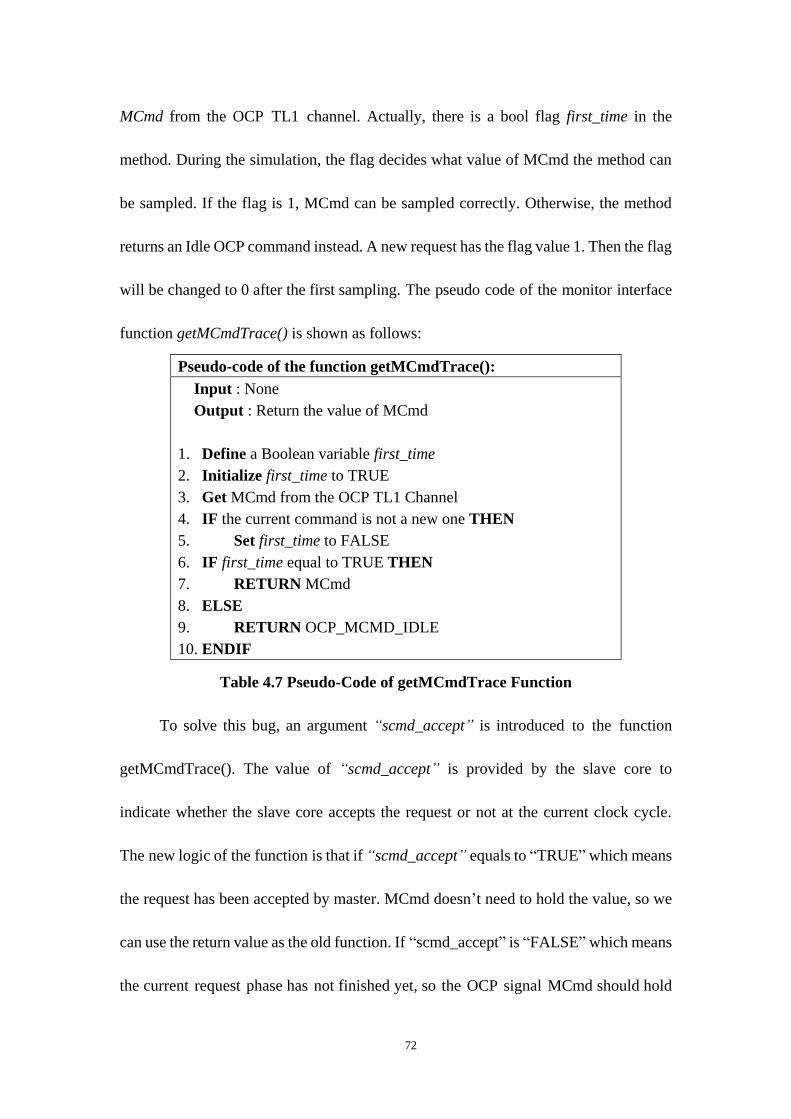
72
MCmd from the OCP TL1 channel. Actually, there is a bool flag first_time in the
method. During the simulation, the flag decides what value of MCmd the method can
be sampled. If the flag is 1, MCmd can be sampled correctly. Otherwise, the method
returns an Idle OCP command instead. A new request has the flag value 1. Then the flag
will be changed to 0 after the first sampling. The pseudo code of the monitor interface
function getMCmdTrace() is shown as follows:
Pseudo-code of the function getMCmdTrace():
Input : None
Output : Return the value of MCmd
1. Define a Boolean variable first_time
2. Initialize first_time to TRUE
3. Get MCmd from the OCP TL1 Channel
4. IF the current command is not a new one THEN
5. Set first_time to FALSE
6. IF first_time equal to TRUE THEN
7. RETURN MCmd
8. ELSE
9. RETURN OCP_MCMD_IDLE
10. ENDIF
Table 4.7 Pseudo-Code of getMCmdTrace Function
To solve this bug, an argument “scmd_accept” is introduced to the function
getMCmdTrace(). The value of “scmd_accept” is provided by the slave core to
indicate whether the slave core accepts the request or not at the current clock cycle.
The new logic of the function is that if “scmd_accept” equals to “TRUE” which means
the request has been accepted by master. MCmd doesn‟t need to hold the value, so we
can use the return value as the old function. If “scmd_accept” is “FALSE” which means
the current request phase has not finished yet, so the OCP signal MCmd should hold

73
the previous command type instead of OCP_MCMD_IDLE. A valid command of the
request should be returned whatever it‟s the first time or not. The pseudo-code of the
modified code is:
Pseudo-code of the function getMCmdTrace():
Input : Boolean parameter scmd_accept provide by the slave core
Output : Return the value of MCmd
1. Define a Boolean variable first_time
2. Initialize first_time to TRUE
3. Get MCmd from the OCP TL1 Channel
4. IF the current command is not a new one THEN
5. Set first_time to FALSE
6. IF scmd_accept is true THEN
7. IF first_time equal to TRUE THEN
8. RETURN MCmd
9. ELSE
10. RETURN OCP_MCMD_IDLE
11. ENDIF
12. ELSE
13. RETURN MCmd
14. ENDIF
Table 4.8 Pseudo-Code of Modified getMCmdTrace Function
Another two similar bugs are also be found which made the two OCP
compliance assertions DataFlow Phase Check 1.2.12 datas_hold_MDataValid and
DataFlow Phase Check 1.2.17 response_hold_SResp [16] fail during the simulation.
We use the same solution to correct the OCP TL1 channel model.
4.2 Random Tests
In this section, random OCP TL1 transactions are generated automatically by
74
both the SCV generator and the CGA module with different random number
generators based on six distribution functions. The simulations are running in the
Advance Verification Environment (AVE) QuestaSim6.4 under WindowsXP SP2
operating system on Intel Core Duo CPU E4500 at 2.2GHz, and with 2GB of RAM.
The OCP functional coverage points are expressed in SystemC for the CGA and in
SystemVerilog for the SCV. In the CGA, the RNGs based on Uniform distribution,
Exponential distribution, Beta distribution, Gamma distribution, Normal distribution
and Triangle distribution are designed as separate C++ classes and are integrated into
the CGA. For different PDFs, different sets of parameters are selected to compare their
effects to the functional coverage rate on the DUV.
In OCP, some of the compliance assertions are very easy to be covered such as
dataflow signal checks. All this kind of assertions is covered in every OCP clock cycle
during the simulation to check if the signals are valid or not. But some dataflow phase
assertions are difficult to be covered for the specific models. The assertion
request_hold_MCmd which we discussed in the previous section is one of them. This
assertion is only reached when MCmd accept backpressure delay happens. Larger the
outstanding request buffer of the OCP slave core is, harder the MCmd accept
backpressure delay is reached.
In this thesis, the OCP TL1 channel is configured to MRMD models as our DUV.
We choose MCmd accept backpressure delay for each OCP thread as our functional
coverage points. Different values of the OCP parameter threads are set to determine the

75
number of functional cover points. Additionally, the outstanding request buffer of the
slave core is set to different values for adjusting the difficult levels of the functional
coverage points to be covered.
4.2.1 OCP Functional Coverage Points
Since the MRMD OCP channel is a multi-thread model, the functional cover
points should be defined as the MCmd accept backpressure delay on every OCP thread.
Because the CGA module is designed in C++, it‟s better to defined functional cover
points in SystemC. With the same language standard, the coverage information can be
easily obtained and analyzed by the evaluation process of CGA. The SystemC code of
the functional coverage points is shown as below:
if(MCmd!=OCP_MCMD_IDLE && MThreadID==i && SCmdAccept==0)
++Covi;
Where
If the signal MCmd is non-idle valid command (MCmd!=OCP_MCMD_IDLE)
and the slave core is not ready to accept the current request (SCmdAccept==0) on the
specified thread (MThreadID==i), the value of the respective coverage point counter
plus one (++Covi). The coverage points are from thread number 0 to .
On the other hand, SCV is employed to generate random OCP transactions to
DUV. Because the SCV generator does not need to collect coverage information and
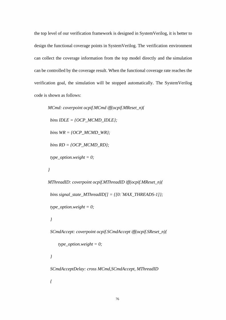
76
the top level of our verification framework is designed in SystemVerilog, it is better to
design the functional coverage points in SystemVerilog. The verification environment
can collect the coverage information from the top model directly and the simulation
can be controlled by the coverage result. When the functional coverage rate reaches the
verification goal, the simulation will be stopped automatically. The SystemVerilog
code is shown as follows:
MCmd: coverpoint ocpif.MCmd iff(ocpif.MReset_n){
bins IDLE = {OCP_MCMD_IDLE};
bins WR = {OCP_MCMD_WR};
bins RD = {OCP_MCMD_RD};
type_option.weight = 0;
}
MThreadID: coverpoint ocpif.MThreadID iff(ocpif.MReset_n){
bins signal_state_MThreadID[] = {[0:`MAX_THREADS-1]};
type_option.weight = 0;
}
SCmdAccept: coverpoint ocpif.SCmdAccept iff(ocpif.SReset_n){
type_option.weight = 0;
}
SCmdAcceptDelay: cross MCmd,SCmdAccept, MThreadID
{
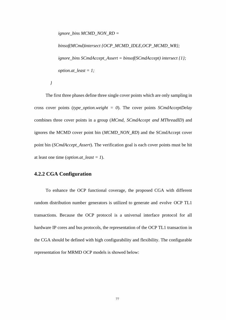
77
ignore_bins MCMD_NON_RD =
binsof(MCmd)intersect {OCP_MCMD_IDLE,OCP_MCMD_WR};
ignore_bins SCmdAccept_Assert = binsof(SCmdAccept) intersect {1};
option.at_least = 1;
}
The first three phases define three single cover points which are only sampling in
cross cover points (type_option.weight = 0). The cover points SCmdAcceptDelay
combines three cover points in a group (MCmd, SCmdAccept and MThreadID) and
ignores the MCMD cover point bin (MCMD_NON_RD) and the SCmdAccept cover
point bin (SCmdAccept_Assert). The verification goal is each cover points must be hit
at least one time (option.at_least = 1).
4.2.2 CGA Configuration
To enhance the OCP functional coverage, the proposed CGA with different
random distribution number generators is utilized to generate and evolve OCP TL1
transactions. Because the OCP protocol is a universal interface protocol for all
hardware IP cores and bus protocols, the representation of the OCP TL1 transaction in
the CGA should be defined with high configurability and flexibility. The configurable
representation for MRMD OCP models is showed below:
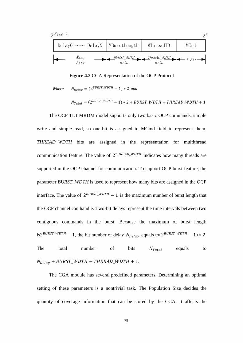
78
Delay0 …… DelayN MBurstLength MThreadID MCmd
NDelay Bits
THREAD_WDTH Bits
1 BitBURST_WDTH
Bits
021
2TotalN
Figure 4.2 CGA Representation of the OCP Protocol
Where and
The OCP TL1 MRDM model supports only two basic OCP commands, simple
write and simple read, so one-bit is assigned to MCmd field to represent them.
THREAD_WDTH bits are assigned in the representation for multithread
communication feature. The value of indicates how many threads are
supported in the OCP channel for communication. To support OCP burst feature, the
parameter BURST_WDTH is used to represent how many bits are assigned in the OCP
interface. The value of is the maximum number of burst length that
the OCP channel can handle. Two-bit delays represent the time intervals between two
contiguous commands in the burst. Because the maximum of burst length
is , the bit number of delay equals to .
The total number of bits equals to
.
The CGA module has several predefined parameters. Determining an optimal
setting of these parameters is a nontrivial task. The Population Size decides the
quantity of coverage information that can be stored by the CGA. It affects the
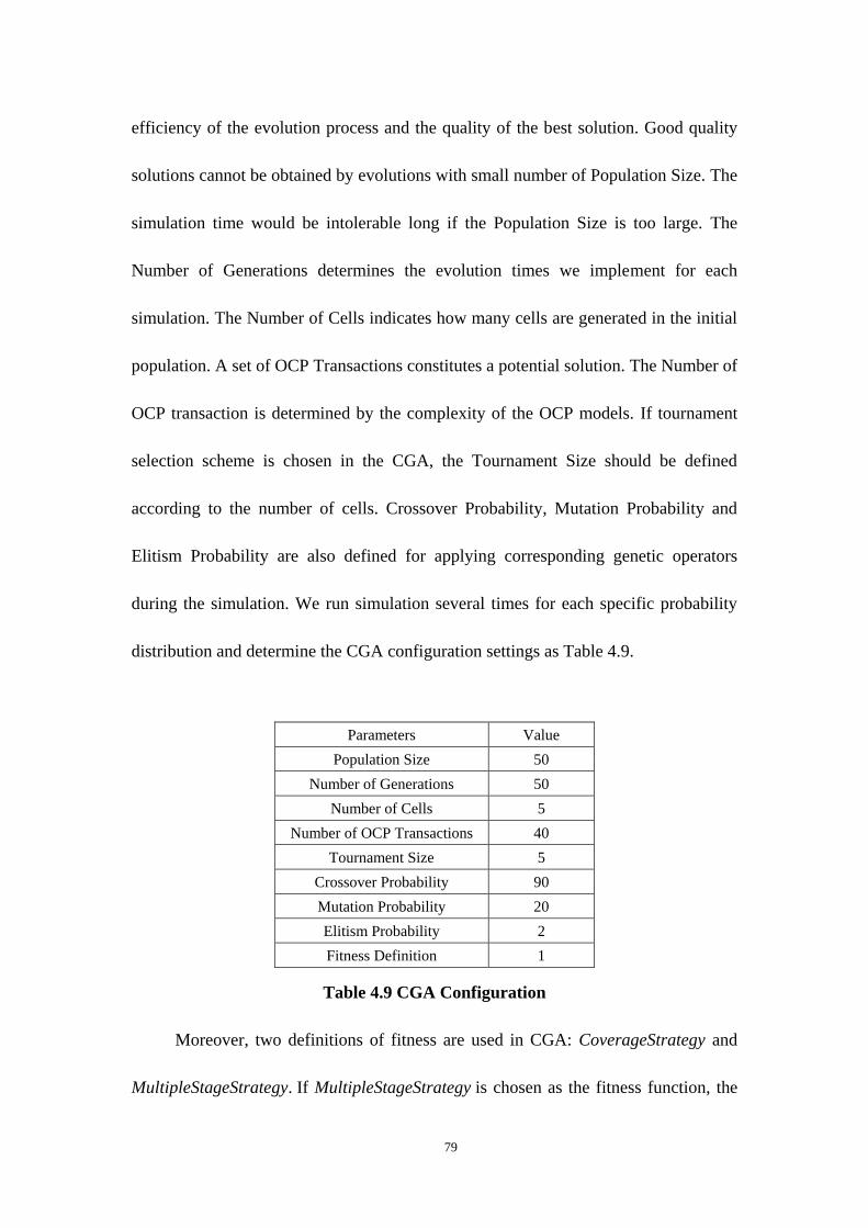
79
efficiency of the evolution process and the quality of the best solution. Good quality
solutions cannot be obtained by evolutions with small number of Population Size. The
simulation time would be intolerable long if the Population Size is too large. The
Number of Generations determines the evolution times we implement for each
simulation. The Number of Cells indicates how many cells are generated in the initial
population. A set of OCP Transactions constitutes a potential solution. The Number of
OCP transaction is determined by the complexity of the OCP models. If tournament
selection scheme is chosen in the CGA, the Tournament Size should be defined
according to the number of cells. Crossover Probability, Mutation Probability and
Elitism Probability are also defined for applying corresponding genetic operators
during the simulation. We run simulation several times for each specific probability
distribution and determine the CGA configuration settings as Table 4.9.
Parameters Value
Population Size 50
Number of Generations 50
Number of Cells 5
Number of OCP Transactions 40
Tournament Size 5
Crossover Probability 90
Mutation Probability 20
Elitism Probability 2
Fitness Definition 1
Table 4.9 CGA Configuration
Moreover, two definitions of fitness are used in CGA: CoverageStrategy and
MultipleStageStrategy. If MultipleStageStrategy is chosen as the fitness function, the

80
parameters in Table 4.10 must be specified as well.
Parameters Value
Fitness Definition 0
StageWeight 1000.0
CoverageRate1 5
CoverageRate2 10
EnableCoverageStage1 1
EnableCoverageStage2 1
Table 4.10 Multiple Stage Strategy Parameters
4.2.3 SCV representation
SCV library is selected as traditional pure random number generator to compare
with our proposed CGA. It provides a smart pointer scv_smart_ptr to generate data
objects of arbitrary data types randomly. The parts of OCP TL1 transaction can be
defined as follows:
scv_smart_ptr<OCPMCmdType> p_cmd;
scv_smart_ptr<int> p_length;
scv_smart_ptr<int> p_thread;
scv_smart_ptr<int> p_delay[MAX_LENGTH];
To generate a random value from a specifying range, the method keep_only can
be used to modify the distribution. In the following code, MAX_LENGTH represents
the maximum of OCP burst length. For instance, when the value of OCP parameter
burst_wdth is 3, the value of MAX_LENGTH should be 7 and the generation range of
the OCP burst length should be from 1 to 7.
81
p_length->keep_only(1,MAX_LENGTH);
p_thread->keep_only(0,m_threads-1);
for(int i=0; i<MAX_LENGTH; i++)
p_delay[i]->keep_only(1,MAX_DELAY);
After that, calling the method next() in the SCV library, a new OCP TL1
transaction can be generated in the specifying range randomly.
p_cmd->next();
p_length->next();
p_thread->next();
for (int i=0; i<*p_length; i++)
p_delay[i]->next();
4.2.4 Experiment I
In this experiment, an OCP TL1 channel with MRMD configuration setting is
selected as our DUV. The DUV is configured to 1-bit command, 3-bits burst width,
3-bits thread width and 14-bits delay. The parameters of the OCP TL1 slave core are
LatencyX=4 and limitreq_max=3. Because the number of OCP threads is eight (3-bit
thread width), eight MCmd accept backpressure delays are considered as functional
coverage points.
Table 4.11 summarizes the result of CGA with CoverageStrategy
implementation. The first column shows the probability distributions and their
parameters. The second column shows the values of the maximum fitness occurring
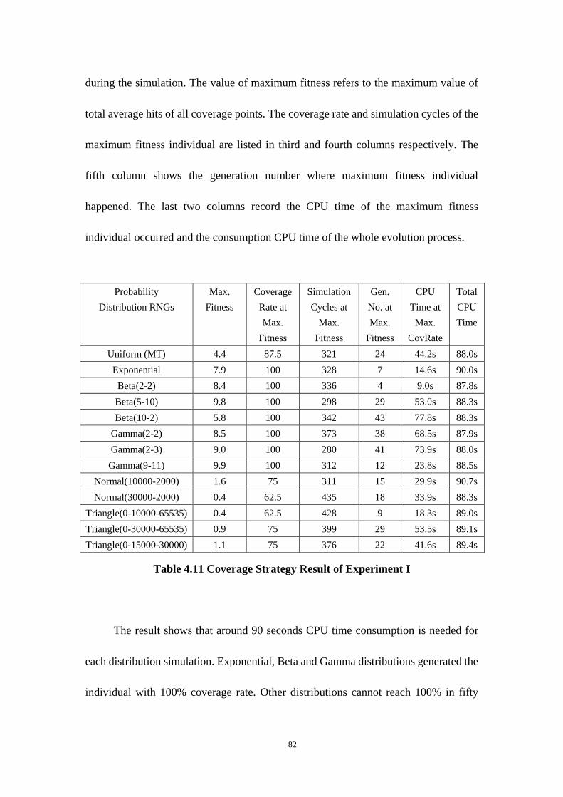
82
during the simulation. The value of maximum fitness refers to the maximum value of
total average hits of all coverage points. The coverage rate and simulation cycles of the
maximum fitness individual are listed in third and fourth columns respectively. The
fifth column shows the generation number where maximum fitness individual
happened. The last two columns record the CPU time of the maximum fitness
individual occurred and the consumption CPU time of the whole evolution process.
Probability
Distribution RNGs
Max.
Fitness
Coverage
Rate at
Max.
Fitness
Simulation
Cycles at
Max.
Fitness
Gen.
No. at
Max.
Fitness
CPU
Time at
Max.
CovRate
Total
CPU
Time
Uniform (MT) 4.4 87.5 321 24 44.2s 88.0s
Exponential 7.9 100 328 7 14.6s 90.0s
Beta(2-2) 8.4 100 336 4 9.0s 87.8s
Beta(5-10) 9.8 100 298 29 53.0s 88.3s
Beta(10-2) 5.8 100 342 43 77.8s 88.3s
Gamma(2-2) 8.5 100 373 38 68.5s 87.9s
Gamma(2-3) 9.0 100 280 41 73.9s 88.0s
Gamma(9-11) 9.9 100 312 12 23.8s 88.5s
Normal(10000-2000) 1.6 75 311 15 29.9s 90.7s
Normal(30000-2000) 0.4 62.5 435 18 33.9s 88.3s
Triangle(0-10000-65535) 0.4 62.5 428 9 18.3s 89.0s
Triangle(0-30000-65535) 0.9 75 399 29 53.5s 89.1s
Triangle(0-15000-30000) 1.1 75 376 22 41.6s 89.4s
Table 4.11 Coverage Strategy Result of Experiment I
The result shows that around 90 seconds CPU time consumption is needed for
each distribution simulation. Exponential, Beta and Gamma distributions generated the
individual with 100% coverage rate. Other distributions cannot reach 100% in fifty
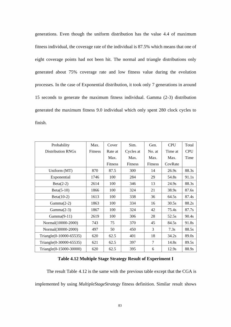
83
generations. Even though the uniform distribution has the value 4.4 of maximum
fitness individual, the coverage rate of the individual is 87.5% which means that one of
eight coverage points had not been hit. The normal and triangle distributions only
generated about 75% coverage rate and low fitness value during the evolution
processes. In the case of Exponential distribution, it took only 7 generations in around
15 seconds to generate the maximum fitness individual. Gamma (2-3) distribution
generated the maximum fitness 9.0 individual which only spent 280 clock cycles to
finish.
Probability
Distribution RNGs
Max.
Fitness
Cover
Rate at
Max.
Fitness
Sim.
Cycles at
Max.
Fitness
Gen.
No. at
Max.
Fitness
CPU
Time at
Max.
CovRate
Total
CPU
Time
Uniform (MT) 870 87.5 300 14 26.9s 88.3s
Exponential 1746 100 284 29 54.8s 91.1s
Beta(2-2) 2614 100 346 13 24.9s 88.3s
Beta(5-10) 1866 100 324 21 38.9s 87.6s
Beta(10-2) 1613 100 338 36 64.5s 87.4s
Gamma(2-2) 1863 100 334 16 30.5s 88.2s
Gamma(2-3) 1867 100 324 42 75.4s 87.7s
Gamma(9-11) 2619 100 306 28 52.5s 90.4s
Normal(10000-2000) 743 75 370 45 84.5s 91.8s
Normal(30000-2000) 497 50 450 3 7.3s 88.5s
Triangle(0-10000-65535) 620 62.5 401 18 34.2s 89.0s
Triangle(0-30000-65535) 621 62.5 397 7 14.8s 89.5s
Triangle(0-15000-30000) 620 62.5 395 6 12.9s 88.9s
Table 4.12 Multiple Stage Strategy Result of Experiment I
The result Table 4.12 is the same with the previous table except that the CGA is
implemented by using MultipleStageStrategy fitness definition. Similar result shows
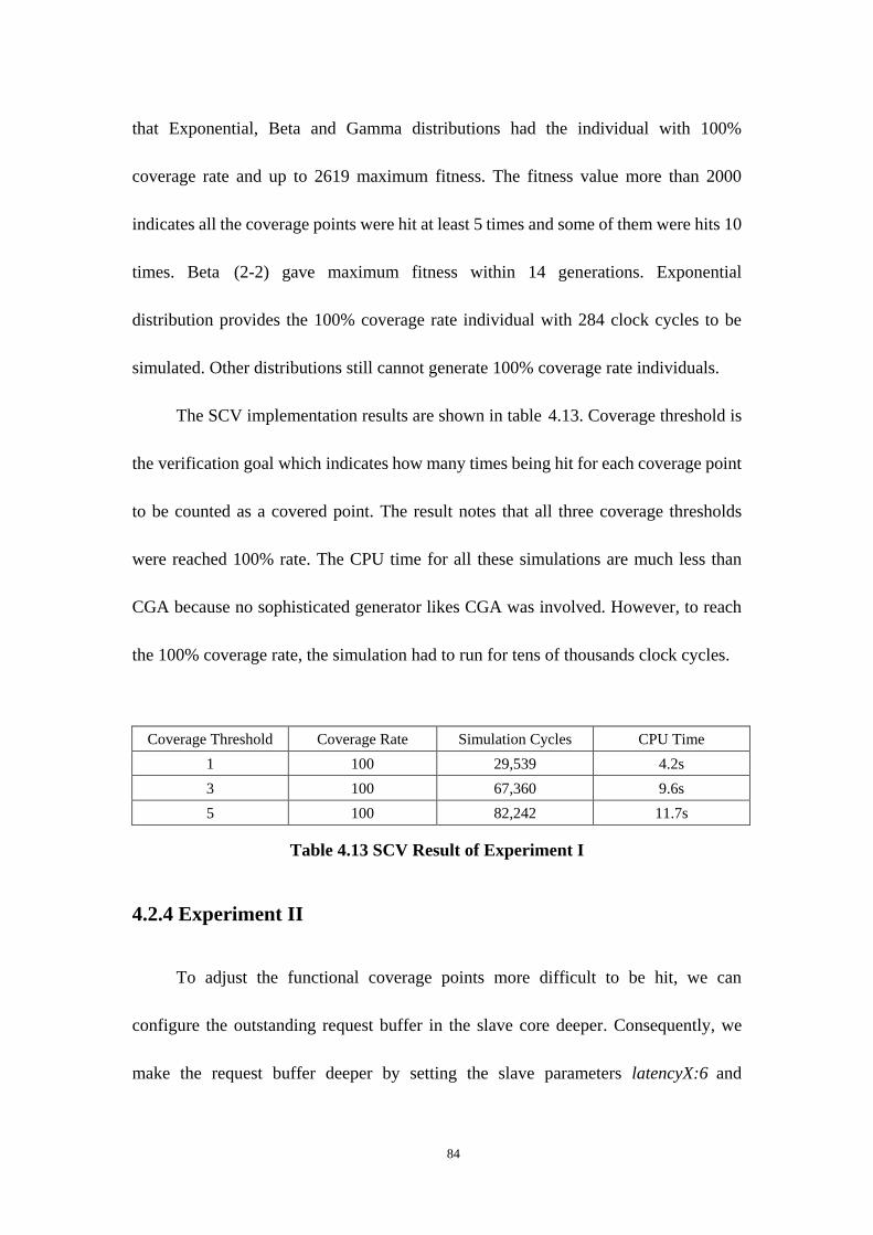
84
that Exponential, Beta and Gamma distributions had the individual with 100%
coverage rate and up to 2619 maximum fitness. The fitness value more than 2000
indicates all the coverage points were hit at least 5 times and some of them were hits 10
times. Beta (2-2) gave maximum fitness within 14 generations. Exponential
distribution provides the 100% coverage rate individual with 284 clock cycles to be
simulated. Other distributions still cannot generate 100% coverage rate individuals.
The SCV implementation results are shown in table 4.13. Coverage threshold is
the verification goal which indicates how many times being hit for each coverage point
to be counted as a covered point. The result notes that all three coverage thresholds
were reached 100% rate. The CPU time for all these simulations are much less than
CGA because no sophisticated generator likes CGA was involved. However, to reach
the 100% coverage rate, the simulation had to run for tens of thousands clock cycles.
Coverage Threshold Coverage Rate Simulation Cycles CPU Time
1 100 29,539 4.2s
3 100 67,360 9.6s
5 100 82,242 11.7s
Table 4.13 SCV Result of Experiment I
4.2.4 Experiment II
To adjust the functional coverage points more difficult to be hit, we can
configure the outstanding request buffer in the slave core deeper. Consequently, we
make the request buffer deeper by setting the slave parameters latencyX:6 and
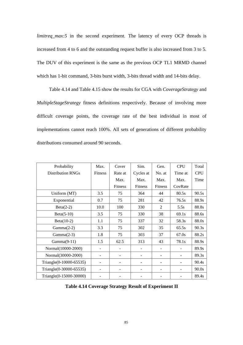
85
limitreq_max:5 in the second experiment. The latency of every OCP threads is
increased from 4 to 6 and the outstanding request buffer is also increased from 3 to 5.
The DUV of this experiment is the same as the previous OCP TL1 MRMD channel
which has 1-bit command, 3-bits burst width, 3-bits thread width and 14-bits delay.
Table 4.14 and Table 4.15 show the results for CGA with CoverageStrategy and
MultipleStageStrategy fitness definitions respectively. Because of involving more
difficult coverage points, the coverage rate of the best individual in most of
implementations cannot reach 100%. All sets of generations of different probability
distributions consumed around 90 seconds.
Probability
Distribution RNGs
Max.
Fitness
Cover
Rate at
Max.
Fitness
Sim.
Cycles at
Max.
Fitness
Gen.
No. at
Max.
Fitness
CPU
Time at
Max.
CovRate
Total
CPU
Time
Uniform (MT) 3.5 75 364 44 80.5s 90.5s
Exponential 0.7 75 281 42 76.5s 88.9s
Beta(2-2) 10.0 100 330 2 5.5s 88.8s
Beta(5-10) 3.5 75 330 38 69.1s 88.6s
Beta(10-2) 1.1 75 337 32 58.3s 88.0s
Gamma(2-2) 3.3 75 302 35 65.5s 90.3s
Gamma(2-3) 1.8 75 303 37 67.0s 88.2s
Gamma(9-11) 1.5 62.5 313 43 78.1s 88.9s
Normal(10000-2000) - - - - - 89.9s
Normal(30000-2000) - - - - - 89.3s
Triangle(0-10000-65535) - - - - - 90.4s
Triangle(0-30000-65535) - - - - - 90.0s
Triangle(0-15000-30000) - - - - - 89.4s
Table 4.14 Coverage Strategy Result of Experiment II
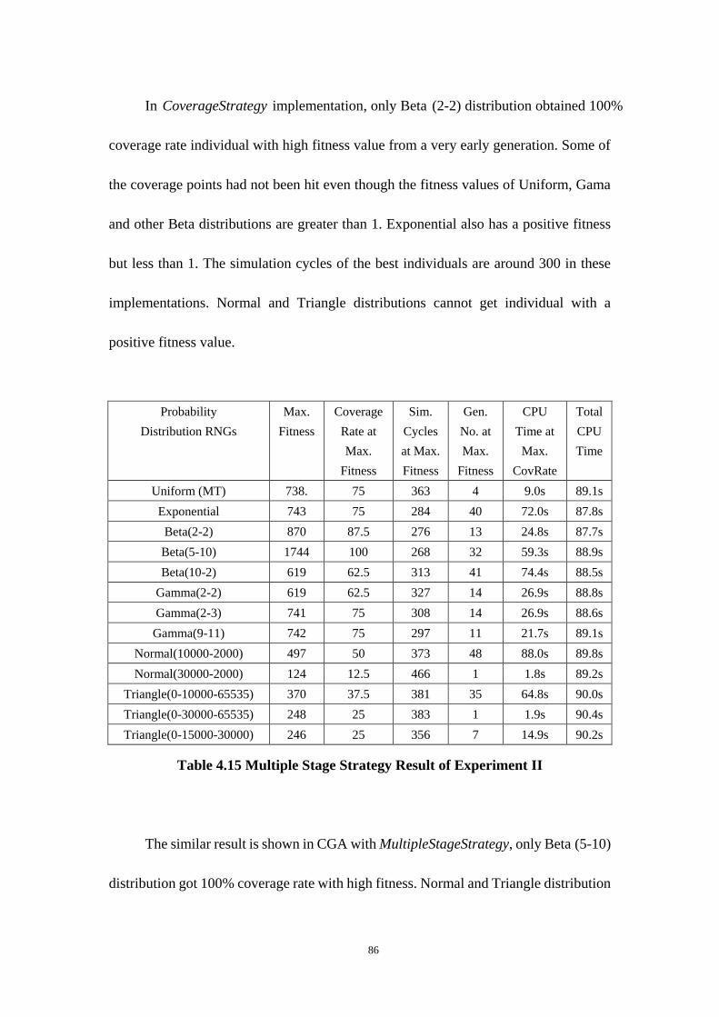
86
In CoverageStrategy implementation, only Beta (2-2) distribution obtained 100%
coverage rate individual with high fitness value from a very early generation. Some of
the coverage points had not been hit even though the fitness values of Uniform, Gama
and other Beta distributions are greater than 1. Exponential also has a positive fitness
but less than 1. The simulation cycles of the best individuals are around 300 in these
implementations. Normal and Triangle distributions cannot get individual with a
positive fitness value.
Probability
Distribution RNGs
Max.
Fitness
Coverage
Rate at
Max.
Fitness
Sim.
Cycles
at Max.
Fitness
Gen.
No. at
Max.
Fitness
CPU
Time at
Max.
CovRate
Total
CPU
Time
Uniform (MT) 738. 75 363 4 9.0s 89.1s
Exponential 743 75 284 40 72.0s 87.8s
Beta(2-2) 870 87.5 276 13 24.8s 87.7s
Beta(5-10) 1744 100 268 32 59.3s 88.9s
Beta(10-2) 619 62.5 313 41 74.4s 88.5s
Gamma(2-2) 619 62.5 327 14 26.9s 88.8s
Gamma(2-3) 741 75 308 14 26.9s 88.6s
Gamma(9-11) 742 75 297 11 21.7s 89.1s
Normal(10000-2000) 497 50 373 48 88.0s 89.8s
Normal(30000-2000) 124 12.5 466 1 1.8s 89.2s
Triangle(0-10000-65535) 370 37.5 381 35 64.8s 90.0s
Triangle(0-30000-65535) 248 25 383 1 1.9s 90.4s
Triangle(0-15000-30000) 246 25 356 7 14.9s 90.2s
Table 4.15 Multiple Stage Strategy Result of Experiment II
The similar result is shown in CGA with MultipleStageStrategy, only Beta (5-10)
distribution got 100% coverage rate with high fitness. Normal and Triangle distribution
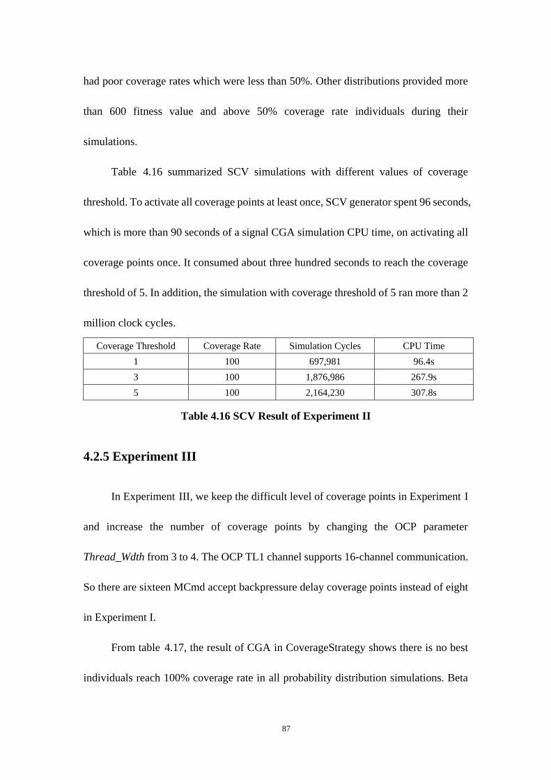
87
had poor coverage rates which were less than 50%. Other distributions provided more
than 600 fitness value and above 50% coverage rate individuals during their
simulations.
Table 4.16 summarized SCV simulations with different values of coverage
threshold. To activate all coverage points at least once, SCV generator spent 96 seconds,
which is more than 90 seconds of a signal CGA simulation CPU time, on activating all
coverage points once. It consumed about three hundred seconds to reach the coverage
threshold of 5. In addition, the simulation with coverage threshold of 5 ran more than 2
million clock cycles.
Coverage Threshold Coverage Rate Simulation Cycles CPU Time
1 100 697,981 96.4s
3 100 1,876,986 267.9s
5 100 2,164,230 307.8s
Table 4.16 SCV Result of Experiment II
4.2.5 Experiment III
In Experiment III, we keep the difficult level of coverage points in Experiment I
and increase the number of coverage points by changing the OCP parameter
Thread_Wdth from 3 to 4. The OCP TL1 channel supports 16-channel communication.
So there are sixteen MCmd accept backpressure delay coverage points instead of eight
in Experiment I.
From table 4.17, the result of CGA in CoverageStrategy shows there is no best
individuals reach 100% coverage rate in all probability distribution simulations. Beta

88
and Gamma distributions obtained the better fitness values than Uniform and
Exponential. Normal and Triangle distribution cannot generate an individual with a
positive fitness value.
Probability
Distribution RNGs
Max.
Fitness
Cover
Rate at
Max.
Fitness
Sim.
Cycles
at Max.
Fitness
Gen.
No. at
Max.
Fitness
CPU
Time at
Max.
CovRate
Total
CPU
Time
Uniform (MT) 0.9 75 298 41 74.5s 89.0s
Exponential 0.6 68.75 312 41 73.4s 87.2s
Beta(2-2) 2.3 75 313 5 10.9s 87.5s
Beta(5-10) 1.8 75 281 25 45.8s 87.6s
Beta(10-2) 1.8 75 344 6 12.6s 89.5s
Gamma(2-2) 1.2 75 306 48 85.4s 87.2s
Gamma(2-3) 2.0 75 344 33 61.1s 89.9s
Gamma(9-11) 1.2 68.75 331 43 77.4s 88.0s
Normal(10000-2000) - - - - - 87.2s
Normal(30000-2000) - - - - 88.7s
Triangle(0-10000-65535) - - - - - 87.8s
Triangle(0-30000-65535) - - - - 87.4s
Triangle(0-15000-30000) - - - - 86.7s
Table 4.17 Coverage Strategy Result of Experiment Three
Table 4.18 shows result of the CGA in MultipleStageStrategy. No individuals
reaches 100% coverage rate. All distributions provided above 50% coverage rate
except Normal and Triangle distributions. Normal and Triangle distributions still
present poor quality of generating OCP TL1 transactions.
Either of the CGA implements provided 100% coverage. The main reason is due
to the fact that it is very difficult to cover sixteen coverage points by an individual with
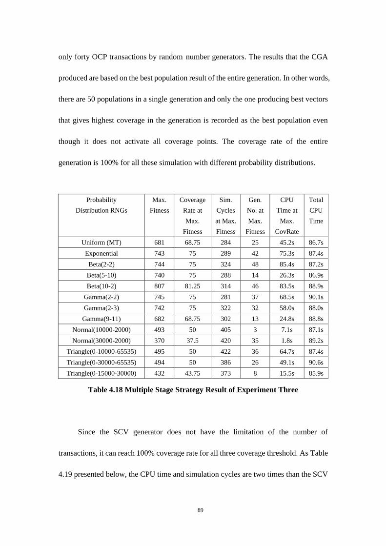
89
only forty OCP transactions by random number generators. The results that the CGA
produced are based on the best population result of the entire generation. In other words,
there are 50 populations in a single generation and only the one producing best vectors
that gives highest coverage in the generation is recorded as the best population even
though it does not activate all coverage points. The coverage rate of the entire
generation is 100% for all these simulation with different probability distributions.
Probability
Distribution RNGs
Max.
Fitness
Coverage
Rate at
Max.
Fitness
Sim.
Cycles
at Max.
Fitness
Gen.
No. at
Max.
Fitness
CPU
Time at
Max.
CovRate
Total
CPU
Time
Uniform (MT) 681 68.75 284 25 45.2s 86.7s
Exponential 743 75 289 42 75.3s 87.4s
Beta(2-2) 744 75 324 48 85.4s 87.2s
Beta(5-10) 740 75 288 14 26.3s 86.9s
Beta(10-2) 807 81.25 314 46 83.5s 88.9s
Gamma(2-2) 745 75 281 37 68.5s 90.1s
Gamma(2-3) 742 75 322 32 58.0s 88.0s
Gamma(9-11) 682 68.75 302 13 24.8s 88.8s
Normal(10000-2000) 493 50 405 3 7.1s 87.1s
Normal(30000-2000) 370 37.5 420 35 1.8s 89.2s
Triangle(0-10000-65535) 495 50 422 36 64.7s 87.4s
Triangle(0-30000-65535) 494 50 386 26 49.1s 90.6s
Triangle(0-15000-30000) 432 43.75 373 8 15.5s 85.9s
Table 4.18 Multiple Stage Strategy Result of Experiment Three
Since the SCV generator does not have the limitation of the number of
transactions, it can reach 100% coverage rate for all three coverage threshold. As Table
4.19 presented below, the CPU time and simulation cycles are two times than the SCV
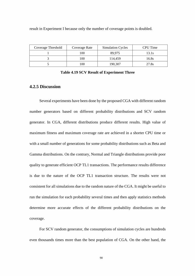
90
result in Experiment I because only the number of coverage points is doubled.
Coverage Threshold Coverage Rate Simulation Cycles CPU Time
1 100 89,975 13.1s
3 100 114,459 16.8s
5 100 190,307 27.8s
Table 4.19 SCV Result of Experiment Three
4.2.5 Discussion
Several experiments have been done by the proposed CGA with different random
number generators based on different probability distributions and SCV random
generator. In CGA, different distributions produce different results. High value of
maximum fitness and maximum coverage rate are achieved in a shorter CPU time or
with a small number of generations for some probability distributions such as Beta and
Gamma distributions. On the contrary, Normal and Triangle distributions provide poor
quality to generate efficient OCP TL1 transactions. The performance results difference
is due to the nature of the OCP TL1 transaction structure. The results were not
consistent for all simulations due to the random nature of the CGA. It might be useful to
run the simulation for each probability several times and then apply statistics methods
determine more accurate effects of the different probability distributions on the
coverage.
For SCV random generator, the consumptions of simulation cycles are hundreds
even thousands times more than the best population of CGA. On the other hand, the
91
CPU time consumptions in SCV are much less than CGA in the relatively small size of
DUV because CGA spends most of time on random number generation and evolution
process. But when the DUV is large system model, the proportion of the CPU time
consumption of CGA will decrease because most of time will be consumed on the
DUV. So the difference of the CPU time consumptions could be ignored in large DUV.
Moreover, it is important to note that the OCP TL1 channel DUV is designed by
SystemC in TLM. TLM modeling allows up to 1000 times faster than RTL modeling.
Lots of time will be saved if we reused the best populations of CGA in RTL models
instead of using the SCV generator directly according to the huge difference between
the number of simulation cycles in CGA and SCV.
Chapter 5
Conclusion and Future Work
5.1 Conclusion
In this thesis, we presented a verification framework which is configurable and
reusable at various levels of hardware model abstraction. The OCP TL1 channel
models with different configuration settings are chosen as DUVs. A universal OCP
SVA monitor along with OCP compliance assertions and functional coverage points is
developed and attached to OCP interface during the simulations. Because of the
extensive usage of SystemVerilog both as a verification and assertion language, the
monitor can be integrated at different development stages of a SoC.
We utilized Cell-based Genetic Algorithm with different random number
generators to improve functional coverage for OCP TL1 models. The integrated
random number generators are based on Exponential, Normal, Gamma, Beta and
Triangle distributions. SystemC Verification library was also employed as random
generator to compare with CGA. The functional coverage points are designed by
SystemC and SystemVerilog languages for CGA and SCV random generators
respectively.
In CGA, different probability distributions have different effects on the
functional coverage. With some distributions, the best population which has high
93
fitness value, high coverage rate and low clock cycle consumptions is generated with a
small number generations. However, with others the best population is obtained after
several generations. The results of all probability distributions show slight difference
due to the random nature of the CGA. It would be good to run the simulation for each
probability distribution RNG several times and then apply statistical method to
determine more accurate effects on the functional coverage. In addition, the fitness
value and functional coverage rate did not improve with some RNGs and fluctuates
around a certain value because of the nature of the functional coverage of the DUVs.
In SCV, the 100% coverage rate is reached with less CPU time consumption but
much longer clock cycle simulations than CGA. The reason is SCV did not involve
complex RNGs and running a single simulation to reach the aim of 100% coverage.
SCV spent less execution time in less CPU time consumption in our small
SystemC TLM DUV. However, CPU time consumption of each clock cycle for RTL
could be 100 even 1000 times more than TLM model. For a large system RTL model
DUV, the consumption of each clock cycle could be very expensive. If the standard
SCV is used directly on such DUV, it executed CPU time to reach good functional
coverage rate would be huge. Instead, if the proposed CGA is utilized on high abstract
level model such as TLM with few more CPU time consumption. Then the best
population of CGA with optimized functional coverage and small number of clock
cycles consumption can be reused in the corresponding RTL model. Therefore, we can
spend a little bit effort on high level hardware models and get great benefit at low

94
level models.
5.2 Future Work
In this thesis, we developed SystemVerilog-based OCP verification framework
utilizing both assertion-based verification methodology and coverage-driven
verification methodology to verify OCP TL1 channel and model. However, the
enhancements can be made by providing configurable OCP CGA generator and
monitor since there are three abstraction level OCP channels. Be configured to
different abstraction levels such as TL3, TL2, TL1 or RTL, the enhanced CGA
generator should be able to generate OCP transactions and evolve functional coverage.
Accordingly, our OCP monitor can be enhanced by adding configurable OCP
assertions and coverage points for different abstraction level designs.
In addition, we provided implementing adapter to divide OCP TL1 transactions
into pin accurate port connections for OCP compliance checks in our OCP monitor.
However, configurable adapters can be added in master side, slave side and monitor
interface. With these configurable adapters, different abstraction layer OCP models
can communicate by different OCP channel. Different abstraction layer OCP
assertions in the monitor can be used to check different layer communication.
Finally, we consider proving the correctness of our framework by integrating it
with a Formal Verification Flow. This will allow re-using the OCP assertions by
transforming them to LTL (Linear Temporal Logic) properties in order to perform

95
Model-Checking.
References
[1] OCP-IP. “Open core protocol international partnership”. http://www.ocpip.org/,
2007.
[2] Thomas Kropf. Introduction to Formal Hardware Verification. Springer-Verlag,
1999.
[3] M.J.C. Gordon and T.F. Melham. Introduction to HOL: A Theorem Proving
Environment for Higher-Order Logic. Cambridge University Press, 1993.
[4] PVS. http://pvs.csl.sri.com, 2008.
[5] J. Bergeron, E. Cerny, A. Hunter, A. Nightingale. Verification Methodology
Manual for SystemVerilog. Springs, 2006
[6] Mentor Graphics. Advanced Verification Methodology Cookbook.
www.mentor.com, 2007.
[7] Sasan Iman. Step by Step Functional Verification with SystemVerilog and
OVM. Hansen Brown Publishing, 2008.
[8] Accellera Organizaion, Inc. SystemVerilog 3.1a Language Reference Manual:
Accellera‟s Extensions to Verilog, 2004.
[9] Srikanth Vijayaraghavan, Meyyappan Ramanathan. A Practical Guide for
SystemVerilog Assertions. Springer, 2005.
[10] OpenVera Assertion Language Reference Manual.
www.open-vera.com/technical/OVAIPGuidelines.pdf.
97
[11] Accellera Property Specification Language Reference Manual (version 1.1).
http://www.eda.org/vfv/docs/PSL-v1.1.pdf.
[12] A. Samara, A. Habibi, S. Tahar, and N. Kharma. Automated Coverage Directed
Test Generation Using Cell-Based Genetic Algorithm. In Proc. of IEEE
International High Level Design Validation and Test Workshop, pages 19-26,
Monterey, California, USA, 2006.
[13] Mike Mintz and Robert Ekendahl. Hardware Verification with SystemVerilog,
May 2007.
[14] SystemC Verification Standard Specification V1.0e. SystemC Verification
Working Group, May 2003.
[15] Chris Spear, Synopsys Inc. SystemVerilog for Verification. Springer, 2006.
[16] OCP-IP. Open Core Protocol Specification Release 2.2, 2006
[17] Intel Corporation. Moores Law. http://www.intel.com/technology/mooreslaw/,
2005.
[18] Atsushi Kasuya and Tesh Tesfaye, “Verification methodologies in a
TLM-to-RTL design flow.” In Proc. IEEE/ACM Design Automation
Conference (DAC 2007), Pages: 199 – 204, San Diego, California, USA, June
2007.
[19] Kun Tong and Jinian Bian, “Assertion-based Performance Analysis for OCP
Systems.” In Proc. Circuits, Signals, and Systems (CSS 2007), Banff, Alberta,
Canada, July 2007.

98
[20] S. Fine and A. Ziv. Coverage Directed Test Generation for Functional
Verification using Bayesian Networks. In Proc. of Design Automation
Conference, pages 286-291, New York, NY, USA, 2003. ACM Press.
[21] H. Shen and Y. Fu. Priority Directed Test Generation for Functional Verification
using Neural Networks. In Proc. of the Conference on Design Automation - Asia
South Pacific, volume 2, pages 1052-1055, Shanghai, China, 2005.
[22] P. Faye, E. Cerny, and P. Pownall. Improved Design Verification by Random
Simulation Guided by Genetic Algorithms. In Proc. of ICDA/APChDL, IFIP
World Computer Congress, pages 456-466, P. R. China, 2000.
[23] M. Bose, J. Shin, E. M. Rudnick and M. Abadir. A Genetic Approach to
Automatic Bias Generation for Biased Random Instruction Generation. In Proc.
Congress on Evolutionary Computation, pages 442-448, Munich, Germany,
2001.
[24] R. Yang, L. Wu, J. Guo, and B. Liu. The Research and Implement of an
Advanced Function Coverage Based Verification Environment. In Proc. of 7th
International Conference on ASIC, pages 1253-1256, Guilin, China, 2007.
[25] Essam Arshed Ahmed. Enhancing Coverage Based Verification using
Probability Distribution. Concordia University, 2008.
[26] Melanie Mitchell. An introduction of genetic algorithms. MIT Press, 1999.
[27] Richard B. Darst. Introduction to Linear Programming. CRC Press, 1990.
[28] Thomas H. Cormen. Introduction to algorithms, Third Edition. MIT, 2009.
99
[29] Donald E. Knuth. The art of computer programming. Addison-Wesley
Professional, 2009.
[30] Zbigniew Michalewicz. Genetic Algorithms + Data Structures = Evolution
Programs. Springer, 1996.
[31] IEEE Standard Association. IEEE Standard SystemC Language Reference
Manual. www.ieee.org, 2006.
[32] J. Bhasker. A SystemC™ Primer. Cadence Design Systems, 2002.
[33] T. Grotker, S. Liao, G. Martin and S. Swan. System Design with SystemC™.
Kluwer Academic Publishers, 2002.
[34] IEEE Standard Association. IEEE Standard for SystemVerilog - Unified
Hardware Design, Specification, and Verification Language. www.ieee.org,
2005.
[35] Transaction Level Modeling using OSCI TLM 2.0. http://www.systemc.org/,
May 31, 2007
[36] M. Spiegel, J. Schiller, and R. Srinivasan. Theory and Problems of Probability
and Statistics. McGraw-Hill, 2000.
[37] Mentor Graphics Corporation, Questa™ SV/AFV User‟s Manual,
2007.
[38] A SystemC OCP Transaction Level Communication Channel V2.2, February 6,
2007
[39] Hamilton B. Carter, Shankar Hemmady. Metric-Driven Design Verification.

100
Springer, 2007.
[40] M. Matsumoto and T. Nishimura. Mersenne Twister: A 623-dimensionally
Equidistance Uniform Pseudo-Random Number Generator. ACM Transaction
on Modeling and Computer Simulation, 8(1):3-30, 1998.
[41] D. T. Lang. Approaches for Random Number Generation. Class notes of
Statistical Computing: STAT 141, http://eeyore.ucdavis.edu/stat141/Notes/
RNG.pdf. University of California at Davis, USA, 2006.
[42] R. Roy. Comparison of Different Techniques to Generate Normal Random
Variables. Technical report. The State University of New Jersey, USA, 2004.
[43] W. Press, B. P. Flannery, S. A. Teukolsky, and W. T. Vetterling. Numerical
Recipes in C: The Art of Scientific Computing. Cambridge University Press,
1992.
[44] Simon Haykin. Neural Networks A Comprehensive Foundation (Second
Edition). Pearson Education, Inc., 2009.
[45] A. H. Warren. Introduction: Special Issue on Microprocessor Verifications.
Formal Methods in System Design, 20:135-137, 2002.