a uni ed approach to structural limits and limits of ...iti.mff.cuni.cz/series/2013/573.pdf · a...
TRANSCRIPT
A Unified Approach to Structural Limits and
Limits of Graphs with Bounded Tree-depth
Jaroslav Nesetril
Patrice Ossona de Mendez
Author address:
Jaroslav Nesetril, Computer Science Institute of Charles Univer-sity (IUUK and ITI), Malostranske nam.25, 11800 Praha 1, Czech Re-public
E-mail address: [email protected]
Patrice Ossona de Mendez, Centre d’Analyse et de MathematiquesSociales (CNRS, UMR 8557), 190-198 avenue de France, 75013 Paris,France
E-mail address: [email protected]

Contents
Chapter 1. Introduction 11.1. Main Definitions and Results 4
Chapter 2. General Theory 92.1. Limits as Measures on Stone Spaces 92.2. Convergence, Old and New 172.3. Combining Fragments 242.4. Interpretation Schemes 35
Chapter 3. Modelings for Sparse Structures 393.1. Relational Samples Spaces 393.2. Modelings 413.3. Decomposing Sequences: the Comb Structure 62
Chapter 4. Limits of Graphs with Bounded Tree-depth 774.1. FO1-limits of Colored Rooted Trees with Bounded Height 774.2. FO-limits of Colored Rooted Trees with Bounded Height 934.3. Limit of Graphs with Bounded Tree-depth 100
Chapter 5. Concluding Remarks 1015.1. Selected Problems 101Acknowledgements 103
Bibliography 105
iii
Abstract
In this paper we introduce a general framework for the study of limits ofrelational structures and graphs in particular, which is based on a combination ofmodel theory and (functional) analysis. We show how the various approaches tograph limits fit to this framework and that they naturally appear as “tractablecases” of a general theory. As an outcome of this, we provide extensions of knownresults. We believe that this put these into next context and perspective. Forexample, we prove that the sparse–dense dichotomy exactly corresponds to randomfree graphons. The second part of the paper is devoted to the study of sparsestructures. First, we consider limits of structures with bounded diameter connectedcomponents and we prove that in this case the convergence can be “almost” studiedcomponent-wise. We also propose the structure of limits objects for convergentsequences of sparse structures. Eventually, we consider the specific case of limits ofcolored rooted trees with bounded height and of graphs with bounded tree-depth,motivated by their role as “elementary bricks” these graphs play in decompositionsof sparse graphs, and give an explicit construction of a limit object in this case.This limit object is a graph built on a standard probability space with the propertythat every first-order definable set of tuples is measurable. This is an exampleof the general concept of modeling we introduce here. Our example is also thefirst “intermediate class” with explicitly defined limit structures where the inverseproblem has been solved.
Received by the editor October 20th, 2013.2010 Mathematics Subject Classification. Primary 03C13 (Finite structures), 03C98 (Appli-
cations of model theory), 05C99 (Graph theory), 06E15 (Stone spaces and related structures),Secondary 28C05 (Integration theory via linear functionals).
Key words and phrases. Graph and Relational structure and Graph limits and Structural lim-
its and Radon measures and Stone space and Model theory and First-order logic and Measurablegraph.
Supported by grant ERCCZ LL-1201 and CE-ITI P202/12/G061, and by the European
Associated Laboratory “Structures in Combinatorics” (LEA STRUCO).Supported by grant ERCCZ LL-1201 and by the European Associated Laboratory “Structures
in Combinatorics” (LEA STRUCO).
iv

CHAPTER 1
Introduction
To facilitate the study of the asymptotic properties of finite graphs (and moregenerally of finite structures) in a sequence G1, G2, . . . , Gn, . . ., it is natural tointroduce notions of structural convergence. By structural convergence, we meanthat we are interested in the characteristics of a typical vertex (or group of vertices)in the graph Gn, as n grows to infinity. This convergence can be concisely expressedby various means. We note two main directions:
• the convergence of the sampling distributions;• the convergence with respect to a metric in the space of structures (such
as the cut metric).
Also, sampling from a limit structure may also be used to define a sequenceconvergent to the limit structure.
All these directions lead to a rich theory which originated in a probabilisticcontext by Aldous [3] and Hoover [42] (see also the monograph of Kallenberg [45]and the survey of Austin [6]) and, independently, in the study of random graphprocesses, and in analysis of properties of random (and quasirandom) graphs (inturn motivated among others by statistical physics [13, 14, 54]). This developmentis nicely documented in the recent monograph of Lovasz [53].
The asymptotic properties of large graphs are studied also in the context ofdecision problems as exemplified e.g. by structural graphs theory, [22, 71]. Howeverit seems that the existential approach typical for decision problems, structural graphtheory and model theory on the one side and the counting approach typical forstatistics and probabilistic approach on the other side have little in common andlead to different directions: on the one side to study, say, definability of variousclasses and the properties of the homomorphism order and on the other side, say,properties of partition functions. It has been repeatedly stated that these twoextremes are somehow incompatible and lead to different area of study (see e.g. [11,40]). In this paper we take a radically different approach which unifies these bothextremes.
We propose here a model which is a mixture of the analytic, model theoretic andalgebraic approach. It is also a mixture of existential and probabilistic approach.Precisely, our approach is based on the Stone pairing 〈φ,G〉 of a first-order formulaφ (with set of free variables Fv(φ)) and a graph G, which is defined by followingexpression
〈φ,G〉 =|(v1, . . . , v|Fv(φ)|) ∈ G|Fv(φ)| : G |= φ(v1, . . . , v|Fv(φ)|)|
|G||Fv(φ)| .
Stone pairing induces a notion of convergence: a sequence of graphs (Gn)n∈Nis FO-convergent if, for every first order formula φ (in the language of graphs), thevalues 〈φ,Gn〉 converge as n→∞. In other words, (Gn)n∈N is FO-convergent if the
1
2 1. INTRODUCTION
probability that a formula φ is satisfied by the graph Gn with a random assignmentof vertices of Gn to the free variables of φ converges as n grows to infinity. We alsoconsider analogously defined X-convergence, where X is a fragment of FO.
Our main result is that this model of FO-convergence is a suitable model forthe analysis of limits of sparse graphs (and particularly of graphs with boundedtree depth). This fits to a broad context of recent research.
For graphs, and more generally for finite structures, there is a class dichotomy:nowhere dense and somewhere dense [69, 65]. Each class of graphs falls in one ofthese two categories. Somewhere dense class C may be characterised by saying thatthere exists a (primitive positive) FO interpretation of all graphs into them. Suchclass C is inherently a class of dense graphs. In the theory of nowhere dense struc-tures [71] there are two extreme conditions related to sparsity: bounded degree andbounded diameter. Limits of bounded degree graphs have been studied thoroughly[8], and this setting has been partialy extended to sparse graphs with far away largedegree vertices [56]. The class of graphs with bounded diameter is considered inSection 3.3 (and leads to a difficult analysis of componentwise convergence). Thisanalysis provides a first-step for the study of limites of graphs with bounded tree-depth. Classes of graphs with bounded tree-depth can be defined by logical termsas well as combinatorially in various ways; the most concise definition is perhapsthat a class of graphs has bounded tree depth if and only if the maximal lengthof a path in every G in the class is bounded by a constant. Graphs with boundedtree-depth play also the role of building blocks of graphs in a nowhere dense class(by means of low tree-depth decompositions [59, 60, 71]). So the solution of limitsfor graphs with bounded tree depth presents a step (and perhaps provides a roadmap) in solving the limit problem for sparse graphs.
We propose here a new type of measurable structure, called modeling, whichextends the notion of graphing, and which we believe is a good candidate for limitobjects of sequence of graphs in a nowhere dense class. The convergence of graphswith bounded tree depth is analysed in detail and this leads to a construction of amodeling limits for those sequences of graphs where all members of the sequencehave uniformly bounded tree depth (see Theorem 4.36). Moreover, we characterizemodelings which are limits of graphs with bounded tree-depth.
There is more to this than meets the eye: We prove that if C is a monotoneclass of graphs such that every FO-convergent sequence has a modeling limit thenthe class C is nowhere dense (see Theorem 3.32). This shows the natural limitationsto modeling FO-limits. To create a proper model for bounded height trees we haveto introduce the model in a greater generality and it appeared that our approachrelates and in most cases generalizes, by properly chosing fragment X of FO, allexisting models of graph limits. For instance, for the fragment X of all existentialfirst-order formulas, X-convergence means that the probability that a structure hasa particular extension property converges. Our approach is encouraged by the deepconnections to the four notions of convergence which have been proposed to studygraph limits in different contexts.
The ultimate goal of the study of structural limits is to provide (as effectively aspossible) limit objects themselves: we would like to find an object which will inducethe limit distribution and encode the convergence. This was done in a few isolatedcases only: For dense graphs Lovasz and Szegedy isolated the notion of graphon: In

1. INTRODUCTION 3
this representation the limit [54, 13] is a symmetric Lebesgue measurable functionW : [0, 1]2 → [0, 1] called graphon.
A representation of the limit (for our second example of bounded degree graphs)is a measurable graphing (notion introduced by Adams [1] in the context of Ergodictheory), that is a standard Borel space with a measure µ and d measure preservingBorel involutions. The existence of such a representation has been made explicitby Elek [28], and relies on the works of Benjamini [8] and Gaboriau [34]. Both ofthese models of convergence are particular cases of our general approach
One of the main issue of our general approach is to determine a representationof FO-limits as measurable graphs. A natural limit object is a standard probabilityspace (V,Σ, µ) together with a graph with vertex set V and edge set E, with theproperty that every first-order definable subset of a power of V is measurable. Thisleads to the notion of relational sample space and to the notion of modelling. Thisnotion seems to be particularly suitable for sparse graphs (and in the full generalityonly for sparse graphs, see Theorem 3.32.).
In this paper, we shed a new light on all these constructions by an approachinspired by functional analysis. The preliminary material and our framework areintroduced in Sections 1.1 and 2.1. The general approach presented in the firstsections of this paper leads to several new results. Let us mention a sample of suchresults.
Central to the theory of graph limits stand random graphs (in the Erdos-Renyimodel [30]): a sequence of random graphs with increasing order and edge proba-bility 0 < p < 1 is almost surely convergent to the constant graphon p [54]. Onthe other hand, it follows from the work of Erdos and Renyi [31] that such a se-quence is almost surely elementarily convergent to an ultra-homogeneous graph,called the Rado graph. We prove that these two facts, together with the quantifierelimination property of ultra-homogeneous graphs, imply that a sequence of ran-dom graphs with increasing order and edge probability 0 < p < 1 is almost surelyFO-convergent, see Section 2.3.4. (However, we know that this limit cannot beneither random free graphon nor modelling, see Theorem 3.32)
We shall prove that a sequence of bounded degree graphs (Gn)n∈N with|Gn| → ∞ is FO-convergent if and only if it is both convergent in the sense ofBenjamini-Schramm and in the sense of elementary convergence. The limit canstill be represented by a graphing, see Sections 2.2.2 and 3.2.6.
Why Stone pairing? We prove that the limit of an FO-convergent sequenceof graphs is a probability measure on the Stone space of the Boolean algebra offirst-order formulas, which is invariant under the action of Sω on this space, seeSection 2.1. Fine interplay of these notions is depicted on Table 1.
Graph limits (in the sense of Lovasz et al.) — and more generally hypergraphlimits — have been studied by Elek and Szegedy [29] through the introduction ofa measure on the ultraproduct of the graphs in the sequence (via Loeb measureconstruction, see [50]). The fundamental theorem of ultraproducts proved by Los[51] implies that the ultralimit of a sequence of graphs is (as a measurable graph)an FO-limit. Thus in this non-standard setting we get FO-limits (almost) for freesee [70]. (However this does not relate to the difficult question of separability.)
We believe that the approach taken in this paper is natural and that it enrichesthe existing notions of limits. In a sense we proceed dually to [11]: We do not view〈φ,G〉 as a “φ test” for G but rather as operator induced by G on the Boolean

4 1. INTRODUCTION
Boolean algebra B(X) Stone Space S(B(X))
Formula φ Continuous function fφ
Vertex v “Type of vertex” T
Graph G statistics of types
=probability measure µG
〈φ,G〉∫fφ(T ) dµG(T )
X-convergent (Gn) weakly convergent µGn
Γ = Aut(B(X)) Γ-invariant measure
Table 1. Some correspondances
algebra of all FO-formulas (or on the subalgebra induced by a fragment X ⊂ FO).It also presents, for example via decomposition techniques (low-tree depth decom-position, see [71]) a promising approach to more general intermediate classes (seethe final comments).
1.1. Main Definitions and Results
If we consider relational structures with signature λ, the symbols of the relationsand constants in λ define the non-logical symbols of the vocabulary of the first-orderlanguage FO(λ) associated to λ-structures. Notice that if λ is at most countablethen FO(λ) is countable. The symbols of variables will be assumed to be takenfrom a countable set x1, . . . , xn, . . . indexed by N. Let u1, . . . , uk be terms. Theset of used free variables of a formula φ will be denoted by Fv(φ) (by saying that avariable xi is “used” in φ we mean that φ is not logically equivalent to a formula inwhich xi does not appear). The formula φxi1 ,...,xik (u1, . . . , uk) denote the formulaobtained by substituting simultaneously the term uj to the free occurences of xijfor j = 1, . . . , k. In the sake of simplicity, we will denote by φ(u1, . . . , uk) thesubstitution φx1,...,xk(u1, . . . , uk).
A relational structure A with signature λ is defined by its domain (or universe)A and relations with names and arities as defined in λ. In the following we willdenote relational structures by bold face letters A,B, . . . and their domains by thecorresponding light face letters A,B, . . .
The key to our approach are the following two definitions.
Definition 1.1 (Stone pairing). Let λ be a signature, let φ ∈ FO(λ) be afirst-order formula with free variables x1, . . . , xp and let A be a finite λ-structure.
PutΩφ(A) = (v1, . . . , vp) ∈ Ap : A |= φ(v1, . . . , vp).

1.1. MAIN DEFINITIONS AND RESULTS 5
We define the Stone pairing of φ and A by
(1.1) 〈φ,A〉 =|Ωφ(A)||A|p .
In other words, 〈φ,A〉 is the probability that φ is satisfied in A when weinterpret the p free variables of φ by p vertices of G chosen randomly, uniformlyand independently. Also, Ωφ(A) is interpreted as the solution set of φ in A.
Note that in the case of a sentence φ (that is a formula with no free variables,thus p = 0), the definition of the Stone pairing reduces to
〈φ,A〉 =
1, if A |= φ;
0, otherwise.
Definition 1.2 (FO-convergence). A sequence (An)n∈N of finite λ-structuresis FO-convergent if, for every formula φ ∈ FO(λ) the sequence (〈φ,An〉)n∈N is(Cauchy) convergent.
In other words, a sequence (An)n∈N is FO-convergent if the sequence of map-pings 〈 · ,An〉 : FO(λ)→ [0, 1] is pointwise-convergent.
The interpretation of the Stone pairing as a probability suggests to extend thisview to more general λ-structures which will be our candidates for limit objects.
Definition 1.3 (Relational sample space). A relational sample space is a re-lational structure A (with signature λ) with extra structure: The domain A of Aof a sample model is a standard Borel space (with Borel σ-algebra ΣA) with theproperty that every subset of Ap that is first-order definable in FO(λ) is measurable(in Ap with respect to the product σ-algebra). For brevity we shall use the sameletter A for structure and relational sample space.
In other words, if A is a relational sample space then for every integer p andevery φ ∈ FO(λ) with p free variables it holds Ωφ(A) ∈ ΣpA.
Definition 1.4 (Modeling). A modeling A is a relational sample space Aequipped with a probability measure (denoted νA). By the abuse of symbols themodelling will be denoted by A (with σ-algebra ΣA and corresponding measureνA). A modeling with signature λ is a λ-modeling.
Remark 1.5. We take time for some comments on the above definitions:
• According to Kuratowski’s isomorphism theorem, the domains of rela-tional sample spaces are Borel-isomorphic to either R, Z, or a finite space.
• Borel graphs (in the sense of Kechris et al. [46]) are generally not model-ings (in our sense) as Borel graphs are only required to have a measurableadjacency relation.
• By equipping its domain with the discrete σ-algebra, every finite λ-structure defines a relational sample space. Considering the uniform prob-ability measure on this space then canonically defines a uniform modeling.
6 1. INTRODUCTION
• It follows immediately from Definition 1.3 that any k-rooting of a relationalsample space is a relational sample space.
We can extend the definition of Stone pairing from finite structures to modelingsas follows.
Definition 1.6 (Stone pairing for modeling). Let λ be a signature, let φ ∈FO(λ) be a first-order formula with free variables x1, . . . , xp and let A be a λ-modeling.
We can define the Stone pairing of φ and A by
(1.2) 〈φ,A〉 =
∫
x∈Ap1Ωφ(A)(x) dνpA(x).
Note that the definition of a modeling is simply tailored to make the expres-sion (1.2) meaningful. Based on this definition, modelings can sometimes be usedas a representation of the limit of an FO-convergent sequence of finite λ-structures.
Definition 1.7. A modeling L is a modeling FO-limit of an FO-convergentsequence (An)n∈N of finite λ-structures if 〈φ ,An〉 converges pointwise to 〈φ ,L〉for every first order formula φ.
As we shall see in Lemma 3.8, a modeling FO-limit of an FO-convergent se-quence (An)n∈N of finite λ-structures is necessarily weakly uniform. It follows thatif a modeling L is a modeling FO-limit then L is either finite or uncountable.
We shall see that not every FO-convergent sequence of finite relational struc-tures admits a modeling FO-limit. In particular we prove:
Theorem 1.8. Let C be a monotone class of finite graphs, such that every FO-convergent sequence of graphs in C has a modeling FO-limit. Then the class C isnowhere dense.
Recall that a class of graphs is monotone if it is closed by the operation oftaking a subgraph, and that a monotone class of graphs C is nowhere dense if, forevery integer p, there exists an integer N(p) such that the p-th subdivision of thecomplete graph KN(p) on N(p) vertices does not belong to C (see [65, 69, 71]).
However, we conjecture that the theorem above expresses exactly when mod-eling FO-limits exist:
Conjecture 1.1. If (Gn)n∈N is an FO-convergent sequence of graphs and ifGn : n ∈ N is a nowhere dense class, then the sequence (Gn)n∈N has a modelingFO-limit.
As a first step, we prove that modeling FO-limits exist in two particular cases,which form in a certain sense the building blocks of nowhere dense classes.
Theorem 1.9. Let C be a integer.
(1) Every FO-convergent sequence of graphs with maximum degree at most Chas a modeling FO-limit;
1.1. MAIN DEFINITIONS AND RESULTS 7
(2) Every FO-convergent sequence of rooted trees with height at most C has amodeling FO-limit.
The first item will be derived from the graphing representation of limits ofBenjamini-Schramm convergent sequences of graphs with bounded maximum de-gree with no major difficulties. Recall that a graphing [1] is a Borel graph G suchthat the following Intrinsic Mass Transport Principle (IMTP) holds:
∀A,B∫
A
degB(x) dx =
∫
B
degA(y)dy,
where the quantification is on all measurable subsets of vertices, and wheredegB(x) (resp. degA(y)) denote the degree in B (resp. in A) of the vertex x (resp.of the vertex y). In other words, the Mass Transport Principle states that if wecount the edges between sets A and B be summing up the degrees in B of verticesin A or by summing up the degrees in A of vertices in B, we should get the sameresult.
Theorem 1.10 (Elek [28]). The Benjamini-Schramm limit of a bounded degreegraph sequence can be represented by a graphing.
A full characterization of the limit objects in this case is not known, and isrelated to the following conjecture.
Conjecture 1.2 (Aldous, Lyons [5]). Every graphing is the Benjamini-Schramm limit of a bounded degree graph sequence.
Equivalently, every unimodular distribution on rooted countable graphs withbouded degree is the Benjamini-Schramm limit of a bounded degree graph sequence.
We conjecture that a similar condition could characterize modeling FO-limitsof sequences of graphs with bounded degree. In this more general setting, we haveto add a new condition, namely to have the finite model property. Recall that aninfinite structure L has the finite model property if every sentence satisfied by Lhas a finite model.
Conjecture 1.3. A modeling is the Benjamini-Schramm limit of a boundeddegree graph sequence if and only if it is a graph with bounded degree, is weaklyuniform, it satisfies both the Intrinsic Mass Transport Principle, and it has thefinite model property.
When handling infinite degrees, we do not expect to be able to keep the IntrinsicMass Transport Principle as is. If a sequence of finite graphs is FO-convergent tosome modeling L then we require the following condition to hold, which we callFinitary Mass Transport Principle (FMTP):
For every measurable subsets of vertices A and B, if it holds degB(x) ≥ a forevery x ∈ A and degA(y) ≤ b for every y ∈ B then a νL(A) ≤ b νL(B).
Note that in the case of modelings with bounded degrees, the Finitary MassTransport Principle is equivalent to the Intrinsic Mass Transport Principle. Also

8 1. INTRODUCTION
note that the above equation holds necessarily when A and B are first-order de-finable, according to the convergence of the Stone pairings and the fact that theFinitary Mass Transport Principle obviously holds for finite graphs.
The second item of Theorem 1.9 will be quite difficult to establish and is themain result of this paper. In this later case, we obtain an inverse theorem:
Theorem 1.11. Every sequence of finite rooted colored trees with height at mostC has a modeling FO-limit that is a rooted colored trees with height at most C, isweakly uniform, and satisfies the Finitary Mass Transport Principle.
Conversely, every rooted colored tree modeling with height at most C that sat-isfies the Finitary Mass Transport Principle is the FO-limit of a sequence of finiterooted colored trees.
By Theorem 1.8, modeling FO-limit do not exist in general. However, we havea general representation of the limit of an FO-convergent sequence of λ-structuresby means of a probability distribution on a compact Polish space Sλ defined fromFO(λ) using Stone duality:
Theorem 1.12. Let λ be a fixed finite or countable signature. Then there existtwo mappings A 7→ µA and φ 7→ K(φ) such that
• A 7→ µA is an injective mapping from the class of finite λ-structures tothe space of regular probability measures on Sλ,
• φ 7→ K(φ) is a mapping from FO(λ) to the set of the clopen subsets of Sλ,
such that for every finite λ-structure A and every first-order formula φ ∈ FO(λ) itholds:
〈φ,A〉 =
∫
Sλ
1K(φ) dµA.
(To prevent risks of notational ambiguity, we shall use µ as root symbol formeasures on Stone spaces and keep ν for measures on modelings.)
Consider an FO-convergent sequence (An)n∈N. Then the pointwise convergenceof 〈 · ,An〉 translates as a weak ∗-convergence of the measures µAn
and we get:
Theorem 1.13. A sequence (An)n∈N of finite λ-structures is FO-convergent ifand only if the sequence (µAn
)n∈N is weakly ∗-convergent.Moreover, if µAn
⇒ µ then for every first-order formula φ ∈ FO(λ) it holds:
∫
Sλ
1K(φ) dµ = limn→∞
〈φ,An〉.
These last two Theorems are established in the next section as a warm up forour general theory.

CHAPTER 2
General Theory
2.1. Limits as Measures on Stone Spaces
In order to prove the representation theorems Theorem 1.12 and Theorem 1.13,we first need to prove a general representation for additive functions on Booleanalgebras.
2.1.1. Representation of Additive Functions. Recall that a Boolean al-gebra B = (B,∧,∨,¬, 0, 1) is an algebra with two binary operations ∨ and ∧, aunary operation ¬ and two elements 0 and 1, such that (B,∨,∧) is a comple-mented distributive lattice with minimum 0 and maximum 1. The two-elementsBoolean algebra is denoted 2.
To a Boolean algebra B is associated a topological space, denoted S(B), whosepoints are the ultrafilters on B (or equivalently the homomorphisms B → 2). Thetopology on S(B) is generated by a sub-basis consisting of all sets
KB(b) = x ∈ S(B) : b ∈ x,where b ∈ B. When the considered Boolean algebra will be clear from context weshall omit the subscript and write K(b) instead of KB(b).
A topological space is a Stone space if it is Hausdorff, compact, and has a basisof clopen subsets. Boolean spaces and Stone spaces are equivalent as formalizedby Stone representation theorem [74], which states (in the language of categorytheory) that there is a duality between the category of Boolean algebras (withhomomorphisms) and the category of Stone spaces (with continuous functions).This justifies to call S(B) the Stone space of the Boolean algebra B. The twocontravariant functors defining this duality are denoted by S and Ω and defined asfollows:
For every homomorphism h : A → B between two Boolean algebra, we definethe map S(h) : S(B)→ S(A) by S(h)(g) = gh (where points of S(B) are identifiedwith homomorphisms g : B → 2). Then for every homomorphism h : A → B, themap S(h) : S(B)→ S(A) is a continuous function.
Conversely, for every continuous function f : X → Y between two Stone spaces,define the map Ω(f) : Ω(Y ) → Ω(X) by Ω(f)(U) = f−1(U) (where elements ofΩ(X) are identified with clopen sets of X). Then for every continuous functionf : X → Y , the map Ω(f) : Ω(Y )→ Ω(X) is a homomorphism of Boolean algebras.
We denote by K = Ω S one of the two natural isomorphisms defined by theduality. Hence, for a Boolean algebra B, K(B) is the set algebra KB(b) : b ∈ B,and this algebra is isomorphic to B.
An ultrafilter of a Boolean algebra B can be considered as a finitely additivemeasure, for which every subset has either measure 0 or 1. Because of the equiv-alence of the notions of Boolean algebra and of set algebra, we define the space
9
10 2. GENERAL THEORY
ba(B) as the space of all bounded additive functions f : B → R. Recall that afunction f : B → R is additive if for all x, y ∈ B it holds
x ∧ y = 0 =⇒ f(x ∨ y) = f(x) + f(y).
The space ba(B) is a Banach space for the norm
‖f‖ba(B) = supx∈B
f(x)− infx∈B
f(x).
(Recall that the ba space of an algebra of sets Σ is the Banach space consisting ofall bounded and finitely additive measures on Σ with the total variation norm.)
Let V (B) be the normed vector space (of so-called simple functions) generatedby the indicator functions of the clopen sets (equipped with supremum norm). Theindicator function of clopen set K(b) (for some b ∈ B) is denoted by 1K(b).
Lemma 2.1. The space ba(B) is the topological dual of V (B)
Proof. One can identify ba(B) with the space ba(K(B)) of finitely additivemeasure defined on the set algebra K(B). As a vector space, ba(B) ≈ ba(K(B))is then clearly the (algebraic) dual of the normed vector space V (B).
The pairing of a function f ∈ ba(B) and a vector X =∑ni=1 ai1K(bi) is defined
by
[f,X] =
n∑
i=1
aif(bi).
That [f,X] does not depend on a particular choice of a decomposition of X followsfrom the additivity of f . We include a short proof for completeness: Assume∑i αi1K(bi) =
∑i βi1K(bi). As for every b, b′ ∈ B it holds f(b) = f(b∧b′)+f(b∧¬b′)
and 1K(b) = 1K(b∧b′) + 1K(b∧¬b′) we can express the two sums as∑j α′j1K(b′j)
=∑j β′j1K(b′j)
(where b′i ∧ b′j = 0 for every i 6= j), with∑i αif(bi) =
∑j α′jf(b′j) and∑
i βif(bi) =∑j β′jf(b′j). As b′i ∧ b′j = 0 for every i 6= j, for x ∈ K(b′j) it holds
α′j = X(x) = β′j . Hence α′j = β′j for every j. Thus∑i αif(bi) =
∑i βif(bi).
Note that X 7→ [f,X] is indeed continuous. Thus ba(B) is the topological dualof V (B).
Lemma 2.2. The vector space V (B) is dense in C(S(B)) (with the uniformnorm).
Proof. Let f ∈ C(S(B)) and let ε > 0. For z ∈ f(S(B)) let Uz be thepreimage by f of the open ball Bε/2(z) of R centered in z. As f is continuous, Uzis a open set of S(B). As K(b) : b ∈ B is a basis of the topology of S(B), Uz canbe expressed as a union
⋃b∈F(Uz)K(b). It follows that
⋃z∈f(S(B))
⋃b∈F(Uz)K(b)
is a covering of S(B) by open sets. As S(B) is compact, there exists a finite subsetF of
⋃z∈f(S(B)) F(Uz) that covers S(B). Moreover, as for every b, b′ ∈ B it holds
K(b) ∩ K(b′) = K(b ∧ b′) and K(b) \ K(b′) = K(b ∧ ¬b′) it follows that we canassume that there exists a finite family F ′ such that S(B) is covered by open setsK(b) (for b ∈ F ′) and such that for every b ∈ F ′ there exists b′ ∈ F such thatK(b) ⊆ K(b′). In particular, it follows that for every b ∈ F ′, f(K(b)) is includedin an open ball of radius ε/2 of R. For each b ∈ F ′ choose a point xb ∈ S(B) suchthat b ∈ xb. Now define
f =∑
b∈F ′f(xb)1K(b)

2.1. LIMITS AS MEASURES ON STONE SPACES 11
Let x ∈ S(B). Then there exists b ∈ F ′ such that x ∈ K(b). Thus
|f(x)− f(x)| = |f(x)− f(xb)| < ε.
Hence ‖f − f‖∞ < ε.
Lemma 2.3. Let B be a Boolean algebra, let ba(B) be the Banach space ofbounded additive real-valued functions equipped with the norm ‖f‖ = supb∈B f(b)−infb∈B f(b), let S(B) be the Stone space associated to B by Stone representationtheorem, and let rca(S(B)) be the Banach space of the regular countably additivemeasure on S(B) equipped with the total variation norm.
Then the mapping CK : rca(S(B)) → ba(B) defined by CK(µ) = µ K is anisometric isomorphism. In other words, CK is defined by
CK(µ)(b) = µ(x ∈ S(B) : b ∈ x)
(considering that the points of S(B) are the ultrafilters on B).
Proof. According to Lemma 2.1, the Banach space ba(B) is the topologicaldual of V (B) and as V (B) is dense in C(S(B)) (according to Lemma 2.2) wededuce that ba(B) can be identified with the continuous dual of C(S(B)). By Rieszrepresentation theorem, the topological dual of C(S(B)) is the space rca(S(B)) ofregular countably additive measures on S(B). ¿From these observations follows theequivalence of ba(B) and rca(S(B)).
This equivalence is easily made explicit, leading to the conclusion that themapping CK : rca(S(B)) → ba(B) defined by CK(µ) = µ K is an isometricisomorphism.
Note also that, similarly, the restriction of CK to the space Pr(S(B)) of all(regular) probability measures on S(B) is an isometric isomorphism of Pr(S(B))and the subset ba1(B) of ba(B) of all positive additive functions f on B such thatf(1) = 1.
Recall that given a measurable function f : X → Y (where X and Y aremeasurable spaces), the pushforward f∗(µ) of a measure µ on X is the measureon Y defined by f∗(µ)(A) = µ(f−1(A)) (for every measurable set A of Y ). Notethat if f is a continuous function and if µ is a regular measure on X, then thepushforward measure f∗(µ) is a regular measure on Y . By similarity with thedefinition of Ω(f) : Ω(Y ) → Ω(X) (see above definition) we denote by Ω∗(f) themapping from rca(X) to rca(Y ) defined by (Ω∗(f))(µ) = f∗(µ).
All the functors defined above are consistent in the sense that if h : A → B isa homomorphism and f ∈ ba(B) then
Ω∗(S(h))(µf ) KA = f h = τh(f).
A standard notion of convergence in rca(S(B)) (as the continuous dual ofC(S(B))) is the weak ∗-convergence: a sequence (µn)n∈N of measures is conver-gent if, for every f ∈ C(S(B)) the sequence
∫f(x) dµn(x) is convergent. Thanks
to the density of V (B) this convergence translates as pointwise convergence inba(B) as follows: a sequence (gn)n∈N of functions in ba(B) is convergent if, forevery b ∈ B the sequence (gn(b))n∈N is convergent. As rca(S(B)) is complete, so isrca(B). Moreover, it is easily checked that ba1(B) is closed in ba(B).
12 2. GENERAL THEORY
In a more concise way, we can write, for a sequence (fn)n∈N of functions inba(B) and for the corresponding sequence (µfn)n∈N of regular measures on S(B):
fn → f pointwise ⇐⇒ µfn ⇒ µf .
We now apply this classical machinery to structures and models.
2.1.2. Basics of Model Theory and Lindenbaum-Tarski Algebras. Wedenote by B(FO(λ)) the equivalence classes of FO(λ) defined by logical equivalence.The (class of) unsatisfiable formulas (resp. of tautologies) will be designated by0 (resp. 1). Then, B(FO(λ)) gets a natural structure of Boolean algebra (withminimum 0, maximum 1, infimum ∧, supremum ∨, and complement ¬). Thisalgbera is called the Lindenbaum-Tarski algebra of FO(λ). Notice that all theBoolean algebras FO(λ) for countable λ are isomorphic, as there exists only onecountable atomless Boolean algebra up to isomorphism (see [41]).
For an integer p ≥ 1, the fragment FOp(λ) of FO(λ) contains first-order for-mulas φ such that Fv(φ) ⊆ x1, . . . , xp. The fragment FO0(λ) of FO(λ) containsfirst-order formulas without free variables (that is sentences).
We check that the permutation group Sp on [p] acts on FOp(λ) by σ · φ =φ(xσ(1), . . . , xσ(p)) and that each permutation indeed define an automorphism ofB(FOp(λ)). Similarly, the group Sω of permutation on N with finite support actson FO(λ) and B(FO(λ)). Note that FO0(λ) ⊆ · · · ⊆ FOp(λ) ⊆ FOp+1(λ) ⊆ · · · ⊆FO(λ). Conversely, let rank(φ) = maxi : xi ∈ Fv(φ). Then we have a naturalprojection πp : FO(λ)→ FOp(λ) defined by
πp(φ) =
φ if rank(φ) ≤ p∃xp+1 ∃xp+2 . . . ∃xrank(φ) φ otherwise
An elementary class (or axiomatizable class) C of λ-structures is a class consist-ing of all λ-structures satisfying a fixed consistent first-order theory TC . Denotingby ITC the ideal of all first-order formulas in L that are provably false from ax-ioms in TC , The Lindenbaum-Tarski algebra B(FO(λ), TC) associated to the theoryTC of C is the quotient Boolean algebra B(FO(λ), TC) = B(FO(λ))/ITC . As a set,B(FO(λ), TC) is simply the quotient of FO(λ) by logical equivalence modulo TC .
As we consider countable languages, TC is at most countable and it is eas-ily checked that S(B(FO(λ), TC)) is homeomorphic to the compact subspace ofS(B(FO(λ)) defined as T ∈ S(B(FO(λ))) : T ⊇ TC. Note that, for instance,S(B(FO0(λ), TC)) is a clopen set of S(B(FO0(λ))) if and only if C is finitely ax-iomatizable (or a basic elementary class), that is if TC can be chosen to be a singlesentence. These explicit correspondences are particularly useful to our setting.
2.1.3. Stone Pairing Again. We add a few comments to Definition 1.6. Notefirst that this definition is consistent in the sense that for every modeling A andfor every formula φ ∈ FO(λ) with p free variables can be considered as a formulawith q ≥ p free variables with q − p unused variables, we have
∫
Aq1Ωφ(A)(x) dνqA(x) =
∫
Ap1Ωφ(A)(x) dνpA(x).
It is immediate that for every formula φ it holds 〈¬φ,A〉 = 1−〈φ,A〉. Moreover,if φ1, . . . , φn are formulas, then by de Moivre’s formula, it holds
2.1. LIMITS AS MEASURES ON STONE SPACES 13
〈n∨
i=1
φi,A〉 =n∑
k=1
(−1)k+1
( ∑
1≤i1<···<ik≤n〈k∧
j=1
φij ,A〉).
In particular, if φ1, . . . , φk are mutually exclusive (meaning that φi ∧ φj = 0)then it holds
〈k∨
i=1
φi,A〉 =k∑
i=1
〈φi,A〉.
It follows that for every fixed modeling A, the mapping φ 7→ 〈φ,A〉 is additive(i.e. 〈 · ,A〉 ∈ ba(B(FO(λ)))):
φ1 ∧ φ2 = 0 =⇒ 〈φ1 ∨ φ2,A〉 = 〈φ1,A〉+ 〈φ2,A〉.The Stone pairing is antimonotone:
Let φ, ψ ∈ FO(λ). For every modeling A it holds
φ ` ψ =⇒ 〈φ,G〉 ≥ 〈ψ,G〉.
However, even if φ and ψ are sentences and 〈φ, · 〉 ≥ 〈ψ, · 〉 on finite λ-structures,this does not imply in general that φ ` ψ: let θ be a sentence with only infinitemodels and let φ be a sentence with only finite models. On finite λ-structures itholds 〈φ ∨ θ, · 〉 = 〈φ, · 〉 although φ ∨ θ 0 φ (as witnessed by an infinite model ofθ).
Nevertheless, inequalities between Stone pairing that are valid for finite λ-structures will of course still hold at the limit. For instance, for φ1, φ2 ∈ FO1(λ),for ζ ∈ FO2(λ), and for a, b ∈ N define the first-order sentence B(a, b, φ1, φ2, ζ)expressing that for every vertex x such that φ1(x) holds there exist at least avertices y such that φ2(y) ∧ ζ(x, y) holds and that for every vertex y such thatφ2(x) holds there exist at most b vertices x such that φ1(x) ∧ ζ(x, y) holds. Thenit is easily checked that for every finite λ-structure A it holds
A |= B(a, b, φ1, φ2, ζ) =⇒ a〈φ1,A〉 ≤ b〈φ2,A〉.For example, if a finite directed graph is such that every arc connects a vertex without-degree 2 to a vertex with in-degree 1, it is clear that the probability that arandom vertex has out-degree 2 is half the probability that a random vertex hasin-degree 1.
Now we come to important twist and the basic of our approach. The Stonepairing 〈 · , · 〉 can be considered from both sides: On the right side the functions oftype 〈φ, · 〉 are a generalization of the homomorphism density functions [11]:
t(F,G) =|hom(F,G)||G||F |
(these functions correspond to 〈φ,G〉 for Boolean conjunctive queries φ and a graphG). Also the density function used in [8] to measure the probability that the ball ofradius r rooted at a random vertex as a given isomorphism type may be expressedas a function 〈φ, · 〉. We follow here, in a sense, a dual approach: from the leftside we consider for fixed A the function 〈 · ,A〉, which is an additive function onB(FO(λ)) with the following properties:
• 〈 · ,A〉 ≥ 0 and 〈1,A〉 = 1;• 〈σ · φ,A〉 = 〈φ, 〉 for every σ ∈ Sω;

14 2. GENERAL THEORY
• if Fv(φ) ∩ Fv(ψ) = ∅, then 〈φ ∧ ψ,A〉 = 〈φ,A〉 〈ψ,A〉.Thus 〈 · ,A〉 is, for a given A, an operator on the class of first-order formulas.We now can apply Lemma 2.3 to derive a representation by means of a regular
measure on a Stone space. The fine structure and interplay of additive functions,Boolean functions, and dual spaces can be used effectively if we consider finite λ-structures as probability spaces as we did when we considered finite λ-structuresas a particular case of Borel models.
The following two theorems generalize Theorems 1.12 and 1.13 mentioned inSection 1.1.
Theorem 2.4. Let λ be a signature, let B(FO(λ)) be the Lindenbaum-Tarski algebra of FO(λ), let S(B(FO(λ))) be the associated Stone space, and letrca(S(B(FO(λ)))) be the Banach space of the regular countably additive measure onS(B(FO(λ))). Then:
(1) There is a mapping from the class of λ-modeling to rca(S(B(FO(λ)))),which maps a modeling A to the unique regular measure µA such that forevery φ ∈ FO(λ) it holds
〈φ,A〉 =
∫
S(B(FO(λ)))
1K(φ) dµA,
where 1K(φ) is the indicator function of K(φ) in S(B(FO(λ))). Moreover,this mapping is injective of finite λ-structures.
(2) A sequence (An)n∈N of finite λ-structures is FO-convergent if and only ifthe sequence (µAn
)n∈N is weakly converging in rca(S(B(FO(λ))));(3) If (An)n∈N is an FO-convergent sequence of finite λ-structures then the
weak limit µ of (µAn)n∈N is such that for every φ ∈ FO(λ) it holds
limn→∞
〈φ,An〉 =
∫
S(B(FO(λ)))
1K(φ) dµ.
Proof. The proof follows from Lemma 2.3, considering the additive functions〈 · ,A〉.
Let A be a finite λ-structure. As µA allows to recover the complete theory ofA and as A is finite, the mapping A 7→ µA is injective.
It is important to consider fragments of FO(λ) to define a weaker notion ofconvergence. This allows us to capture limits of dense graphs too.
Definition 2.5 (X-convergence). Let X be a fragment of FO(λ). A sequence(An)n∈N of finite λ-structures is X-convergent if 〈φ,An〉 is convergent for everyφ ∈ X.
In the particular case that X is a Boolean sub algebra of B(FO(λ)) we canapply all above methods and in this context we can extend Theorem 2.4.
Theorem 2.6. Let λ be a signature, and let X be a fragment of FO(λ) defininga Boolean algebra B(X) ⊆ B(FO(λ)). Let S(B(X)) be the associated Stone space,and let rca(S(B(X))) be the Banach space of the regular countably additive measureon S(B(X)). Then:

2.1. LIMITS AS MEASURES ON STONE SPACES 15
(1) The canonical injection ιX : B(X) → B(FO(λ)) defines by duality a con-tinuous projection pX : S(B(FO(λ)))→ S(B(X)); The pushforward pX∗ µA
of the measure µA associated to a modeling A (see Theorem 2.4) is theunique regular measure on S(B(X)) such that:
〈φ,A〉 =
∫
S(B(X))
1K(φ) dpX∗ µA,
where 1K(φ) is the indicator function of K(φ) in S(B(X)).(2) A sequence (An)n∈N of finite λ-structures is X-convergent if and only if
the sequence (pX∗ µAn)n∈N is weakly converging in rca(S(B(X)));(3) If (An)n∈N is an X-convergent sequence of finite λ-structures then the
weak limit µ of (pX∗ µAn)n∈N is such that for every φ ∈ X it holds
limn→∞
〈φ,An〉 =
∫
S(B(X))
1K(φ) dµ.
Proof. If X is closed under conjunction, disjunction and negation, thus defin-ing a Boolean algebra B(X), then the inclusion of X in FO(λ) translates as acanonical injection ι from B(X) to B(FO(λ)). By Stone duality, the injection ιcorresponds to a continuous projection p : S(B(FO(λ))) → S(B(X)). As everymeasurable function, this continuous projection also transports measures by push-forward: the projection p transfers the measure µ on S(B(FO(λ))) to S(B(X)) asthe pushforward measure p∗µ defined by the identity p∗µ(Y ) = µ(p−1(Y )), whichholds for every measurable subset Y of S(B(X)).
The proof follows from Lemma 2.3, considering the additive functions 〈 · ,A〉.
We can also consider a notion of convergence restricted to λ-structures satisfy-ing a fixed axiom.
Theorem 2.7. Let λ be a signature, and let X be a fragment of FO(λ) defininga Boolean algebra B(X) ⊆ B(FO(λ)). Let S(B(X)) be the associated Stone space,and let rca(S(B(X))) be the Banach space of the regular countably additive measureon S(B(X)).
Let C be a basic elementary class defined by a single axiom Ψ ∈ X ∩ FO0, andlet IΨ be the principal ideal of B(X) generated by ¬Ψ.
Then:
(1) The Boolean algebra obtained by taking the quotient of X equivalencemodulo Ψ is the quotient Boolean algebra B(X,Ψ) = B(X)/IΨ. ThenS(B(X,Ψ)) is homeomorphic to the clopen subspace K(Ψ) of S(B(X)).
If A ∈ C is a finite λ-structure then the support of the measure pX∗ µA
associated to A (see Theorem 2.6) is included in K(Ψ) and for everyφ ∈ X it holds
〈φ,A〉 =
∫
K(Ψ)
1K(φ) dpX∗ µA.
(2) A sequence (An)n∈N of finite λ-structures of C is X-convergent if and onlyif the sequence (pX∗ µAn)n∈N is weakly converging in rca(S(B(X,Ψ)));

16 2. GENERAL THEORY
(3) If (An)n∈N is an X-convergent sequence of finite λ-structures in C thenthe weak limit µ of (pX∗ µAn)n∈N is such that for every φ ∈ X it holds
limn→∞
〈φ,An〉 =
∫
K(Ψ)
1K(φ) dµ.
Proof. The quotient algebra B(X,Ψ) = B(X)/IΨ is isomorphic to the sub-Boolean algebra B′ of B of all (equivalence classes of) formulas φ ∧ Ψ for φ ∈ X.To this isomorphism corresponds by duality the identification of S(B(X,Ψ)) withthe clopen subspace K(Ψ) of S(B(X)).
The situation expressed by these theorems is summarized in the following dia-gram.
B(FO(λ))OO
B(X)OO
canonical injectionoo B′inclusionooOO
oo isomorphism // B(X,Ψ)OO
S(B(FO(λ)))
projection pX // S(B(X)) K(Ψ)inclusionoo S(B(X,Ψ))//homeomorphismoo
µpushforward // pX∗ µ
restriction // pX∗ µ
The essence of our approach is that we follow a dual path: we view a graph G asan operator on first-order formulas through Stone pairing 〈 · , G〉.
2.1.4. Limit of Measures Associated to Finite Structures. We considera signature λ and fragment FOp of FO(λ). Let (An)n∈N be an X-convergent se-quence of λ-structures, let µAn be the measure on S(B(X)) associated to An, andlet µ be the weak limit of µAn .
Fact 2.8. As we consider countable languages only, S(B(FOp)) is a Radonspace and thus for every (Borel) probability measure µ on S(B(FOp)), any measur-able set outside the support of µ has zero µ-measure.
Definition 2.9. Let π be the natural projection S(B(FOp))→ S(B(FO0)).A measure µ on S(B(FOp)) is pure if |π(Supp(µ))| = 1. The unique element T
of π(Supp(µ)) is then called the complete theory of µ.
Remark 2.10. Every measure µ that is the weak limit of some sequence ofmeasures associated to finite structures is pure and its complete theory has thefinite model property.
Definition 2.11. For T ∈ S(B(FOp), ψ, φ ∈ FOp, and β ∈ FO2p define
degβ+ψ (T ) =
k if T 3 (∃=k(y1, . . . , yp)β(x1, . . . , xp, y1, . . . , yp) ∧ ψ(y1, . . . , yp))
∞ otherwise.
degβ−φ (T ) =
k if T 3 (∃=k(x1, . . . , xp)φ(x1, . . . , xp) ∧ β(x1, . . . , xp, y1, . . . , yp))
∞ otherwise.

2.2. CONVERGENCE, OLD AND NEW 17
If µ is a measure associated to a finite structure then for every φ, ψ ∈ FOp itholds ∫
K(φ)
degβ+
ψ (T ) dµ(T ) =
∫
K(ψ)
degβ−φ (T ) dµ(T ).
Hence for every measure µ that is the weak limit of some sequence of measuresassociated to finite structures the following property holds:
General Finitary Mass Transport Principle (GFMTP)
For every φ, ψ ∈ FOp, every β ∈ FO2p, and every integers a, b that are such that∀T ∈ K(φ) degβ
+
ψ (T ) ≥ a∀T ∈ K(ψ) degβ−φ (T ) ≤ b
it holdsaµ(K(φ)) ≤ b µ(K(ψ)).
Of course, similar statement holds as well for the projection of µ on S(B(FOq))for q < p. In the case of digraphs, when p = 1 and β(x1, x2) is existence of an arc
from x1 to x2, we shall note deg+ψ and deg−φ instead of degβ+
ψ and degβ−φ . (In the
case of graphs, we have deg+ψ = deg−ψ = degψ.) Thus it holds
Finitary Mass Transport Principle (FMTP)
For every φ, ψ ∈ FO1, and every integers a, b that are such that∀T ∈ K(φ) deg+
ψ (T ) ≥ a∀T ∈ K(ψ) deg−φ (T ) ≤ b
it holdsaµ(K(φ)) ≤ b µ(K(ψ)).
GFMTP and FMTP will play a key role in the analysis of modeling limits.
2.2. Convergence, Old and New
As we have seen above, there are many ways how to say that a sequence(An)n∈N of finite λ-structures is convergent. As we considered λ-structures de-fined with a countable signature λ, the Boolean algebra B(FO(λ)) is countable. Itfollows that the Stone space S(B(FO(λ))) is a Polish space thus (with the Borelσ-algebra) it is a standard Borel space. Hence every probability distribution turnsS(B(FO(λ))) into a standard probability space. However, the fine structure ofS(B(FO(λ))) is complex and we have no simple description of this space.
FO-convergence is of course the most restrictive notion of convergence and itseems (at least on the first glance) that this is perhaps too much to ask, as we mayencounter many particular difficulties and specific cases. But we shall exhibit laterclasses for which FO-convergence is captured — for special basic elementary classesof structures — by X-convergence for a small fragment X of FO.
At this time it is natural to ask whether one can consider fragments that arenot sub-Boolean algebras of FO(L) and still have a description of the limit of aconverging sequence as a probability measure on a nice measurable space. There isobviously a case where this is possible: when the convergence of 〈φ,An〉 for everyφ in a fragment X implies the convergence of 〈ψ,An〉 for every ψ in the minimum
18 2. GENERAL THEORY
Boolean algebra containing X. We prove now that this is for instance the casewhen X is a fragment closed under conjunction.
We shall need the following preliminary lemma:
Lemma 2.12. Let X ⊆ B be closed by ∧ and such that X generates B (i.e.such that B[X] = B).
Then 1b : b ∈ X ∪ 1 (where 1 is the constant function with value 1)includes a basis of the vector space V (B) generated by the whole set 1b : b ∈ B.
Proof. Let b ∈ B. As X generates B there exist b1, . . . , bk ∈ X and a Booleanfunction F such that b = F (b1, . . . , bk). As 1x∧y = 1x 1y and 1¬x = 1 − 1xthere exists a polynomial PF such that 1b = PF (1b1 , . . . ,1bk). For I ⊆ [k], themonomial
∏i∈I 1bi rewrites as 1bI where bI =
∧i∈I bi. It follows that 1b is a linear
combination of the functions 1bI (I ⊆ [k]) which belong to X if I 6= ∅ (as X isclosed under ∧ operation) and equal 1, otherwise.
Proposition 2.1. Let X be a fragment of FO(λ) closed under (finite) con-junction — thus defining a meet semilattice of B(FO(λ)) — and let B(X) be thesub-Boolean algebra of B(FO(λ)) generated by X. Let X be the fragment of FO(λ)consisting of all formulas with equivalence class in B(X).
Then X-convergence is equivalent to X-convergence.
Proof. Let Ψ ∈ X. According to Lemma 2.12, there exist φ1, . . . , φk ∈ X andα0, α1, . . . , αk ∈ R such that
1Ψ = α01 +k∑
i=1
αi1φi .
Let A be a λ-structure, let Ω = S(B(X)) and let µA ∈ rca(Ω) be the associatedmeasure. Then
〈Ψ,A〉 =
∫
Ω
1Ψ dµA =
∫
Ω
(α01 +
k∑
i=1
αi1φi)
dµG = α0 +k∑
i=1
αi〈φi,A〉.
It follows that if (An)n∈N is an X-convergent sequence, the sequence(〈ψ,An〉)n∈N converges for every ψ ∈ X, that is (An)n∈N is X-convergent.
Now we demonstrate the expressive power of X-convergence by relating it tothe main types of convergence of graphs studied previously:
(1) the notion of dense graph limit [12, 54];(2) the notion of bounded degree graph limit [8, 5];(3) the notion of elementary limit derived from two important results in first-
order logic, namely Godel’s completeness theorem and the compactnesstheorem.
These standard notions of graph limits, which have inspired this work, corre-spond to special fragments of FO(λ), where γ is the signature of graphs. In theremaining of this section, we shall only consider undirected graphs, thus we shallomit to precise their signature in the notations as well as the axiom defining thebasic elementary class of undirected graphs.

2.2. CONVERGENCE, OLD AND NEW 19
2.2.1. L-convergence and QF-convergence. Recall that a sequence(Gn)n∈N of graphs is L-convergent if
t(F,Gn) =hom(F,Gn)
|Gn||F |
converges for every fixed (connected) graph F , where hom(F,G) denotes the numberof homomorphisms of F to G [54, 13, 14].
It is a classical observation that homomorphisms between finite structures canbe expressed by Boolean conjunctive queries [16]. We denote by HOM the fragmentof FO consisting of formulas formed by conjunction of atoms. For instance, theformula
(x1 ∼ x2) ∧ (x2 ∼ x3) ∧ (x3 ∼ x4) ∧ (x4 ∼ x5) ∧ (x5 ∼ x1)
belongs to HOM and it expresses that (x1, x2, x3, x4, x5) form a homomorphic imageof C5. Generally, to a finite graph F we associate the canonical formula φF ∈ HOMdefined by
φF :=∧
ij∈E(F )
(xi ∼ xj).
Then, for every graph G it holds
〈φF , G〉 =hom(F,G)
|G||F | = t(F,G).
Thus L-convergence is equivalent to HOM-convergence. According to Propo-sition 2.1, HOM-convergence is equivalent to HOM-convergent. It is easy to seethat HOM is the fragment QF− of quantifier free formulas that do not use equality.We prove now that HOM-convergence is actually equivalent to QF-convergence,where QF is the fragment of all quantifier free formulas. Note that QF is a properfragment of FOlocal.
Theorem 2.13. Let (Gn) be a sequence of finite graphs such thatlimn→∞ |Gn| =∞.
Then the following conditions are equivalent:
(1) the sequence (Gn) is L-convergent;(2) the sequence (Gn) is QF−-convergent;(3) the sequence (Gn) is QF-convergent;
Proof. As L-convergence is equivalent to HOM-convergence and as HOM ⊂QF− ⊂ QF, it is sufficient to prove that L-convergence implies QF-convergence.
Assume (Gn) is L-convergent. The inclusion-exclusion principle implies thatfor every finite graph F the density of induced subgraphs isomorphic to F convergestoo. Define
dens(F,Gn) =(#F ⊆i Gn)
|Gn||F |.
Then dens(F,Gn) is a converging sequence for each F .Let θ be a quantifier-free formula with Fv(θ) ⊆ [p]. We first consider all possible
cases of equalities between the free variables. For a partition P = (I1, . . . , Ik) of
20 2. GENERAL THEORY
[p], we define |P| = k and sP(i) = min Ii (for 1 ≤ i ≤ |P|). Consider the formula
ζP :=
|P|∧
i=1
(∧
j∈Ii(xj = xsP(i)) ∧
|P|∧
j=i+1
(xsP(j) 6= xsP(i))
).
Then θ is logically equivalent to
(∧
i6=j(xi 6= xj) ∧ θ) ∨
∨
P:|P|<pζP ∧ θP(xsP(1), . . . , xsP(|P|)).
Note that all the formulas in the disjunction are mutually exclusive. Also∧i6=j(xi 6= xj) ∧ θ may be expressed as a disjunction of mutually exclusive terms:
∧
i 6=j(xi 6= xj) ∧ θ =
∨
F∈Fθ′F ,
where F is a finite family of finite graphs F and where G |= θ′F (v1, . . . , vp) if andonly if the mapping i 7→ vi is an isomorphism from F to G[v1, . . . , vp].
It follows that for every graph G it holds:
〈θ,G〉 =∑
F∈F〈θ′F , G〉+
∑
P:|P|<p〈ζP ∧ θP(xsP(1), . . . , xsP(|P|)), G〉
=∑
F∈F〈θ′F , G〉+
∑
P:|P|<p|G||P|−p〈θP , G〉
=∑
F∈F
1
p!
∑
σ∈Sp
|(v1, . . . , vp) : G |= θ′F (vσ(1), . . . , vσ(p))||G|p +O(|G|−1)
=∑
F∈F
Aut(F )
p!dens(F,G) +O(|G|−1).
Thus 〈θ,Gn〉 converge for every quantifier-free formula θ. Hence (Gn) is QF-convergent.
Notice that the condition that limn→∞ |Gn| is necessary as witnessed by thesequence (Gn) where Gn is K1 if n is odd and 2K1 if n is even. The sequenceis obviously L-convergent, but not QF convergent as witnessed by the formulaφ(x, y) : x 6= y, which has density 0 in K1 and 1/2 in K2.
Remark 2.14. The Stone space of the fragment QF− has a simple description.Indeed, a homomorphism h : B(QF−) → 2 is determined by its values on theformulas xi ∼ xj and any mapping from this subset of formulas to 2 extends (in a
unique way) to a homomorphism of B(QF−) to 2. Thus the points of S(B(QF−))
can be identified with the mappings from(N
2
)to 0, 1 that is to the graphs on N.
Hence the considered measures µ are probability measures of graphs on N that havethe property that they are invariant under the natural action of Sω on N. Suchrandom graphs on N are called infinite exchangeable random graphs. For more oninfinite exchangeable random graphs and graph limits, see e.g. [6, 21].

2.2. CONVERGENCE, OLD AND NEW 21
2.2.2. BS-convergence and FOlocal-convergence. The class of graphs withmaximum degree at most D (for some integer D) received much attention. Specifi-cally, the notion of local weak convergence of bounded degree graphs was introducedin [8], which is called here BS-convergence:
A rooted graph is a pair (G, o), where o ∈ V (G). An isomorphism of rootedgraph φ : (G, o) → (G′, o′) is an isomorphism of the underlying graphs whichsatisfies φ(o) = o′. Let D ∈ N. Let GD denote the collection of all isomorphismclasses of connected rooted graphs with maximal degree at most D. For the sake ofsimplicity, we denote elements of GD simply as graphs. For (G, o) ∈ GD and r ≥ 0let BG(o, r) denote the subgraph of G spanned by the vertices at distance at mostr from o. If (G, o), (G′, o′) ∈ GD and r is the largest integer such that (BG(o, r), o)is rooted-graph isomorphic to (BG′(o
′, r), o′), then set ρ((G, o), (G′, o′)) = 1/r, say.Also take ρ((G, o), (G, o)) = 0. Then ρ is metric on GD. Let MD denote the spaceof all probability measures on GD that are measurable with respect to the Borelσ-field of ρ. Then MD is endowed with the topology of weak convergence, and iscompact in this topology.
A sequence (Gn)n∈N of finite connected graphs with maximum degree at mostD is BS-convergent if, for every integer r and every rooted connected graph (F, o)with maximum degree at most D the following limit exists:
limn→∞
|v : BGn(v, r) ∼= (F, o)||Gn|
.
This notion of limits leads to the definition of a limit object as a probabilitymeasure on GD [8].
To relate BS-convergence to X-convergence, we shall consider the fragment oflocal formulas:
Let r ∈ N. A formula φ ∈ FOp is r-local if, for every graph G and everyv1, . . . , vp ∈ Gp it holds
G |= φ(v1, . . . , vp) ⇐⇒ G[Nr(v1, . . . , vp)] |= φ(v1, . . . , vp),
where G[Nr(v1, . . . , vp)] denotes the subgraph of G induced by all the vertices at(graph) distance at most r from one of v1, . . . , vp in G.
A formula φ is local if it is r-local for some r ∈ N; the fragment FOlocal is theset of all local formulas in FO. Notice that if φ1 and φ2 are local formulas, so areφ1 ∧ φ2, φ1 ∨ φ2 and ¬φ1. It follows that the quotient of FOlocal by the relation oflogical equivalence defines a sub-Boolean algebra B(FOlocal) of B(FO). For p ∈ Nwe further define FOlocal
p = FOlocal ∩ FOp.
Theorem 2.15. Let (Gn) be a sequence of finite graphs with maximum degreed, with limn→∞ |Gn| =∞.
Then the following properties are equivalent:
(1) the sequence (Gn)n∈N is BS-convergent;
(2) the sequence (Gn)n∈N is FOlocal1 -convergent;
(3) the sequence (Gn)n∈N is FOlocal-convergent.
Proof. If (Gn)n∈N is FOlocal-convergent, it is FOlocal1 -convergent;

22 2. GENERAL THEORY
If (Gn)n∈N is FOlocal1 -convergent then it is BS-convergent as for any finite rooted
graph (F, o), testing whether the the ball of radius r centered at a vertex x isisomorphic to (F, o) can be formulated by a local first order formula.
Assume (Gn)n∈N is BS-convergent. As we consider graphs with maximumdegree d, there are only finitely many isomorphism types for the balls of radius rcentered at a vertex. It follows that any local formula ξ(x) with a single variablecan be expressed as the conjunction of a finite number of (mutually exclusive)formulas ξ(F,o)(x), which in turn correspond to subgraph testing. It follows that
BS-convergence implies FOlocal1 -convergence.
Assume (Gn)n∈N is FOlocal1 -convergent and let φ ∈ FOlocal
p be an r-local for-mula. Let Fφ be the set of all p-tuples ((F1, f1), . . . , (Fp, fp)) of rooted connectedgraphs with maximum degree at most d and radius (from the root) at most r suchthat
⋃i Fi |= φ(f1, . . . , fp).
Then, for every graph G the sets
Ωφ(G) = (v1, . . . , vp) : G |= φ(v1, . . . , vp)and
⊎
((F1,f1),...,(Fp,fp))∈Fφ
p∏
i=1
v : G |= θ(Fi,fi)(v)
differ by at most O(|G|p−1) elements. Indeed, according to the definition of anr-local formula, the p-tuples (x1, . . . , xp) belonging to exactly one of these sets aresuch that there exists 1 ≤ i < j ≤ p such that dist(xi, xj) ≤ 2r.
It follows that
〈φ,G〉 =( ∑
((Fi,fi))1≤i≤p∈Fφ
p∏
i=1
〈θ(Fi,fi), G〉)
+O(|G|−1).
It follows that FOlocal1 -convergence (hence BS-convergence) implies full FOlocal-
convergence.
Remark 2.16. According to this proposition and Theorem 2.7, the BS-limit ofa sequence of graphs with maximum degree at most D corresponds to a probabilitymeasure on S(B(FOlocal
1 )) whose support is include in the clopen set K(ζD), whereζD is the sentence expressing that the maximum degree is at most D. The Booleanalgebra B(FOlocal
1 ) is isomorphic to the Boolean algebra defined by the fragmentX ⊂ FO0(λ1) of sentences for rooted graphs that are local with respect to the root(here, λ1 denotes the signature of graphs augmented by one symbol of constant).According to this locality, any two countable rooted graphs (G1, r1) and (G2, r2),the trace of the complete theories of (G1, r1) and (G2, r2) on X are the same if andonly if the (rooted) connected component (G′1, r1) of (G1, r1) containing the root r1
is elementary equivalent to the (rooted) connected component (G′2, r2) of (G2, r2)containing the root r2. As isomorphism and elementary equivalence are equivalentfor countable connected graphs with bounded degrees (see Lemma 2.18) it is easilychecked that KX(ζD) is homeomorphic to GD. Hence our setting (while based ona very different and dual approach) leads essentially to the same limit object as [8]for BS-convergent sequences.

2.2. CONVERGENCE, OLD AND NEW 23
2.2.3. Elementary-convergence and FO0-convergence. We already men-tioned that FO0-convergence is nothing but elementary convergence. Elementaryconvergence is implicitly part of the classical model theory. Although we only con-sider graphs here, the definition and results indeed generalize to general λ-structuresWe now reword the notion of elementary convergence:
A sequence (Gn)n∈N is elementarily convergent if, for every sentence φ ∈ FO0,there exists a integer N such that either all the graphs Gn (n ≥ N) satisfy φ ornone of them do.
Of course, the limit object (as a graph) is not unique in general and formally,the limit of an elementarily convergent sequence of graphs is an elementary classdefined by a complete theory.
Elementary convergence is also the backbone of all the X-convergences weconsider in this paper. The FO0-convergence is induced by an easy ultrametricdefined on equivalence classes of elementarily equivalent graphs. Precisely, two(finite or infinite) graphs G1, G2 are elementarily equivalent (denoted G1 ≡ G2) if,for every sentence φ it holds
G1 |= φ ⇐⇒ G2 |= φ.
In other words, two graphs are elementarily equivalent if they satisfy the samesentences.
A weaker (parametrized) notion of equivalence will be crucial: two graphsG1, G2 are k-elementarily equivalent (denoted G1 ≡k G2) if, for every sentence φwith quantifier rank at most k it holds G1 |= φ ⇐⇒ G2 |= φ.
It is easily checked that for every two graphs G1, G2 it holds:
G1 ≡ G2 ⇐⇒ (∀k ∈ N) G1 ≡k G2.
For every fixed k ∈ N, checking whether two graphs G1 and G2 are k-elementarilyequivalent can be done using the so-called Ehrenfeucht-Fraısse game.
¿From the notion of k-elementary equivalence naturally derives a pseudometricdist0(G1, G2):
dist0(G1, G2) =
0 if G1 ≡ G2
min2−qrank(φ) : (G1 |= φ) ∧ (G2 |= ¬φ) otherwise
Proposition 2.2. The metric space of countable graphs (up to elementaryequivalence) with ultrametric dist0 is compact.
Proof. This is a direct consequence of the compactness theorem for first-orderlogic (a theory has a model if and only if every finite subset of it has a model) andof the downward Lowenheim-Skolem theorem (if a theory has a model and thelanguage is countable then the theory has a countable model).
Note that not every countable graph is (up to elementary equivalence) the limitof a sequence of finite graphs. A graph G that is a limit of a sequence finite graphsis said to have the finite model property, as such a graph is characterized by theproperty that every finite set of sentences satisfied by G has a finite model (whatdoes not imply that G is elementarily equivalent to a finite graph).
Example 2.17. A ray is not an elementary limit of finite graphs as it containsexactly one vertex of degree 1 and all the other vertices have degree 2, what can be

24 2. GENERAL THEORY
expressed in first-order logic but is satisfied by no finite graph. However, the unionof two rays is an elementary limit from the sequence (Pn)n∈N of paths of order n.
Although two finite graphs are elementary equivalent if and only if they are iso-morphic, this property does not holds in general for countable graphs. For instance,the union of a ray and a line is elementarily equivalent to a ray. However we shallmake use of the equivalence of isomorphisms and elementary equivalences for rootedconnected countable locally finite graphs, which we prove now for completeness.
Lemma 2.18. Let (G, r) and (G′, r′) be two rooted connected countable graphs.If G is locally finite then (G, r) ≡ (G′, r′) if and only if (G, r) and (G′, r′) are
isomorphic.
Proof. If two rooted graphs are isomorphic they are obviously elementarilyequivalent. Assume that (G, r) and (G′, r′) are elementarily equivalent. Enumeratethe vertices of G in a way that distance to the root is not decreasing. Using n-back-and-forth equivalence (for all n ∈ N), one builds a tree of partial isomorphisms ofthe subgraphs induced by the n first vertices, where ancestor relation is restriction.This tree is infinite and has only finite degrees. Hence, by Konig’s lemma, it containsan infinite path. It is easily checked that it defines an isomorphism from (G, r) to(G′, r′) as these graphs are connected.
Fragments of FO0 allow to define convergence notions, which are weaker thatelementary convergence. The hierarchy of the convergence schemes defined by sub-algebras of B(FO0) is as strict as one could expect. Precisely, if X ⊂ Y are twosub-algebras of B(FO0) then Y -convergence is strictly stronger than X-convergence— meaning that there exists graph sequences that are X-convergent but not Y -convergent — if and only if there exists a sentence φ ∈ Y such that for everysentence ψ ∈ X, there exists a (finite) graph G disproving φ↔ ψ.
We shall see that the special case of elementary convergent sequences is ofparticular importance. Indeed, every limit measure is a Dirac measure concentratedon a single point of S(B(FO0)). This point is the complete theory of the elementarylimit of the considered sequence. This limit can be represented by a finite orcountable graph. As FO-convergence (and any FOp-convergence) implies FO0-convergence, the support of a limit measure µ corresponding to an FOp-convergentsequence (or to an FO-convergent sequence) is such that Supp(µ) projects to asingle point of S(B(FO0)).
Finally, let us remark that all the results of this section can be readily formu-lated and proved for λ-structures.
2.3. Combining Fragments
2.3.1. The FOp Hierarchy. When we consider FOp-convergence of finiteλ-structures for finite a signature λ, the space S(B(FOp(λ))) can be given thefollowing ultrametric distp (compatible with the topology of S(B(FOp(λ)))): LetT1, T2 ∈ S(B(FOp(λ))) (where the points of S(B(FOp(λ))) are identified with ul-trafilters on B(FOp(λ))). Then
distp(T1, T2) =
0 if T1 = T2
2−minqrank(φ): φ∈T1\T2 otherwise
This ultrametric has several other nice properties:
2.3. COMBINING FRAGMENTS 25
• actions of Sp on S(B(FOp(λ))) are isometries:
∀σ ∈ Sp ∀T1, T2 ∈ S(B(FOp(λ))) distp(σ · T1, σ · T2) = distp(T1, T2);
• projections πp are contractions:
∀q ≥ p ∀T1, T2 ∈ S(B(FOq(λ))) distp(πp(T1), πp(T2)) ≤ distq(T1, T2);
We prove that there is a natural isometric embedding ηp : S(B(FOp(λ))) →S(B(FO(λ))). This may be seen as follows: for an ultrafilter X ∈ S(B(FOp(λ))),consider the filter X+ on B(FO(λ)) generated by X and all the formulas xi = xi+1
(for i ≥ p). This filter is an ultrafilter: for every sentence φ ∈ FO(λ), let φ bethe sentence obtained from φ by replacing each free occurrence of a variable xqwith q > p by xp. It is clear that φ and φ are equivalent modulo the theory
Tp = (xi = xi+1) : i ≥ p. As either φ or ¬φ belongs to X, either φ or ¬φ belongs
to ηp(X). Moreover, we deduce easily from the fact that φ and φ have the samequantifier rank that if q ≥ p then πq ηp is an isometry. Finally, let us note thatπp ηp is the identity of S(B(FOp(λ))).
Let λp be the signature λ augmented by p symbols of constants c1, . . . , cp.There is a natural isomorphism of Boolean algebras νp : FOp(λ)→ FO0(λp), whichreplaces the free occurrences of the variables x1, . . . , xp in a formula φ ∈ FOp by thecorresponding symbols of constants c1, . . . , cp, so that it holds, for every modelingA, for every φ ∈ FOp and every v1, . . . , vp ∈ A:
A |= φ(v1, . . . , vp) ⇐⇒ (A, v1, . . . , vp) |= νp(φ).
This mapping induces an isometric isomorphism of the metric spaces(S(B(FOp(λ))),distp) and (S(B(FO0(λp))),dist0). Note that the Stone spaceS(B(FO0(λp))) associated to the Boolean algebra B(FO0(λp)) is the space of allcomplete theories of λp-structures. In particular, points of S(B(FOp(λ)) can berepresented (up to elementary equivalence) by countable λ-structures with p specialpoints. All these transformations may seem routine but they need to be carefullyformulated and checked.
We can test whether the distance distp of two theories T and T ′ is smaller than2−n by means of an Ehrenfeucht-Fraısse game: Let νp(T ) = νp(φ) : φ ∈ T and,similarly, let νp(T
′) = νp(φ) : φ ∈ T ′. Let (A, v1, . . . , vp) be a model of T and let(A′, v′1, . . . , v
′p) ba a model of T ′. Then it holds
distp(T, T′) < 2−n ⇐⇒ (A, v1, . . . , vp) ≡n (A′, v′1, . . . , v
′p).
Recall that the n-rounds Ehrenfeucht-Fraısse game on two λ-structures A andA′, denoted EF(A,A′, n) is the perfect information game with two players — theSpoiler and the Duplicator — defined as follows: The game has n rounds and eachround has two parts. At each round, the Spoiler first chooses one of A and A′ andaccordingly selects either a vertex x ∈ A or a vertex y ∈ A′. Then, the Duplicatorselects a vertex in the other λ-structure. At the end of the n rounds, n vertices havebeen selected from each structure: x1, . . . , xn in A and y1, . . . , yn in A′ (xi and yicorresponding to vertices x and y selected during the ith round). The Duplicatorwins if the substructure induced by the selected vertices are order-isomorphic (i.e.xi 7→ yi is an isomorphism of A[x1, . . . , xn] and A′[y1, . . . , yn]). As there areno hidden moves and no draws, one of the two players has a winning strategy, andwe say that that player wins EF(A,A′, n). The main property of this game is the

26 2. GENERAL THEORY
following equivalence, due to Fraısse [32, 33] and Ehrenfeucht [27]: The duplicatorwins EF(A,A′, n) if and only if A ≡n A′. In our context this translates to thefollowing equivalence:
distp(T, T′) < 2−n ⇐⇒ Duplicator wins EF((A, v1, . . . , vp), (A
′, v′1, . . . , v′p), n).
As FO0 ⊂ FO1 ⊂ · · · ⊂ FOp ⊂ FOp+1 ⊂ · · · ⊂ FO =⋃i FOi, the fragments FO
form a hierarchy of more and more restrictive notions of convergence. In particular,FOp+1-convergence implies FOp-convergence and FO-convergence is equivalent toFOp for all p. If a sequence (An)n∈N is FOp-convergent then for every q ≤ p theFOq-limit of (An)n∈N is a measure µq ∈ rca(S(B(FOq))), which is the pushforwardof µp by the projection πq (more precisely, by the restriction of πq to S(B(FOp))):
µq = (πq)∗(µp).
2.3.2. FOlocal and Locality. FO-convergence can be reduced to the conjunc-tion of elementary convergence and FOlocal-convergence, which we call local con-vergence. This is a consequence of a result, which we recall now:
Theorem 2.19 (Gaifman locality theorem [35]). For every first-order formulaφ(x1, . . . , xn) there exist integers t and r such that φ is equivalent to a Booleancombination of t-local formulas ξs(xi1 , . . . , xis) and sentences of the form
(2.1) ∃y1 . . . ∃ym( ∧
1≤i<j≤mdist(yi, yj) > 2r ∧
∧
1≤i≤mψ(yi)
)
where ψ is r-local. Furthermore, we can choose
r ≤ 7qrank(φ)−1, t ≤ (7qrank(φ)−1 − 1)/2, m ≤ n+ qrank(φ),
and, if φ is a sentence, only sentences (2.1) occur in the Boolean combination.Moreover, these sentences can be chosen with quantifier rank at most q(qrank(φ)),for some fixed function q.
¿From this theorem and the following folklore technical result will follow theclaimed decomposition of FO-convergence into elementary and local convergence.
Lemma 2.20. Let B be a Boolean algebra, let A1 and A2 be sub-Boolean algebrasof B, and let b ∈ B[A1 ∪ A2] be a Boolean combination of elements from A1 andA2. Then b can be written as
b =∨
i∈Ixi ∧ yi,
where I is finite, xi ∈ A1, yi ∈ A2, and for every i 6= j in I it holds (xi∧yi)∧ (xj ∧yj) = 0.
Proof. Let b = F (u1, . . . , ua, v1, . . . , vb) with ui ∈ A1 (1 ≤ i ≤ a) and vj ∈ A2
(1 ≤ j ≤ b) where F is a Boolean combination. By using iteratively Shannon’sexpansion, we can write F as
F (u1, . . . , ua, v1, . . . , vb) =∨
(X1,X2,Y1,Y2)∈F(∧
i∈X1
ui ∧∧
i∈X2
¬ui ∧∧
j∈Y1
vj ∧∧
j∈Y2
¬vj),
where F is a subset of the quadruples (X1, X2, Y1, Y2) such that (X1, X2) is a par-tition of [a] and (Y1, Y2) is a partition of [b]. For a quadruple Q = (X1, X2, Y1, Y2),define xQ =
∧i∈X1
ui ∧∧i∈X2
¬ui and yQ =∧j∈Y1
vj ∧∧j∈Y2¬vj . Then for

2.3. COMBINING FRAGMENTS 27
every Q ∈ F it holds xQ ∈ A1, yQ ∈ A2, for every Q 6= Q′ ∈ F it holdsxQ ∧ yQ ∧ xQ′ ∧ yQ′ = 0, and we have b =
∨Q∈F xQ ∧ yQ.
Theorem 2.21. Let (An) be a sequence of finite λ-structures. Then (An)
is FO-convergent if and only if it is both FOlocal-convergent and FO0-convergent.Precisely, (An) is FOp-convergent if and only if it is both FOlocal
p -convergent andFO0-convergent.
Proof. Assume (An)n∈N is both FOlocalp -convergent and FO0-convergent and
let φ ∈ FOp. According to Theorem 2.19, there exist integers t and r such that φis equivalent to a Boolean combination of t-local formula ξ(xi1 , . . . , xis) and of sen-
tences. As both FOlocal and FO0 define a sub-Boolean algebra of B(FO), according
to Lemma 2.20, φ can be written as∨i∈I ψi ∧ θi, where I is finite, ψi ∈ FOlocal,
θi ∈ FO0, and ψi ∧ θi ∧ ψj ∧ θj = 0 if i 6= j. Thus for every finite λ-structure A itholds
〈φ,A〉 =∑
i∈I〈ψi ∧ θi,A〉.
As 〈 · ,A〉 is additive and 〈θi,A〉 ∈ 0, 1 we have 〈ψi ∧ θi,A〉 = 〈ψi,A〉 〈θi,A〉.Hence
〈φ,A〉 =∑
i∈I〈ψi,A〉 〈θi,A〉.
Thus if (An)n∈N is both FOlocalp -convergent and FO0-convergent then (An)n∈N is
FOp-convergent.
Similarly that points of S(B(FOp(λ)) can be represented (up to elemen-tary equivalence) by countable λ-structures with p special points, points of
S(B(FOlocalp (λ)) can be represented by countable λ-structures with p special points
such that every connected component contains at least one special point. In partic-ular, points of S(B(FOlocal
1 (λ)) can be represented by rooted connected countableλ-structures.
Also, the structure of an FOlocal2 -limit of graphs can be outlined by considering
that points of S(B(FOlocal2 )) as countable graphs with two special vertices c1 and c2,
such that every connected component contains at least one of c1 and c2. Let µ2 bethe limit probability measure on S(B(FOlocal
2 )) for an FOlocal2 -convergent sequence
(Gn)n∈N, let π1 be the standard projection of S(B(FOlocal2 )) into S(B(FOlocal
1 )),
and let µ1 be the pushforward of µ2 by π1. We construct a measurable graph G asfollows: the vertex set of G is the support Supp(µ1) of µ1. Two vertices x and y
of G are adjacent if there exists x′ ∈ π−11 (x) and y′ ∈ π−1
1 (y) such that (considered
as ultrafilters of B(FOlocal2 )) it holds:
• x1 ∼ x2 belongs to both x′ and y′,• the transposition τ1,2 exchanges x′ and y′ (i.e. y′ = τ1,2 · x′).
The vertex set of G is of course endowed with a structure of a probability space(as a measurable subspace of S(B(FOlocal
1 )) equipped with the probability measure
µ1). In the case of bounded degree graphs, the obtained graph G is the graph ofgraphs introduced in [52]. Notice that this graph may have loops. An example ofsuch a graph is shown Fig. 1.

28 2. GENERAL THEORY
2−1
2−2
2−3
2−4
2−5
. . .
S(B(FOlocal1 ))
Figure 1. An outline of the local limit of a sequence of trees
2.3.3. Component-Local Formulas. It is sometimes possible to reduceFOlocal to a smaller fragment. This is in particular the case when connected com-ponents of the considered structures can be identified by some first-order formula.Precisely:
Definition 2.22. Let λ be a signature and let T be a theory of λ-structures.A binary relation $ ∈ λ is a component relation in T if T entails that $ is anequivalence relation such that for every k-ary relation R ∈ λ with k ≥ 2 it holds
T |= (∀x1, . . . , xk)(R(x1, . . . , xk)→
∧
1≤i<j≤k$(xi, xj)
).
A local formula φ with p free variables is $-local if φ is equivalent (modulo T )to φ ∧∧xi,xj∈Fv(φ)$(xi, xj).
In presence of a component relation, it is possible to reduce from FOlocal to thefragment of $-local formulas, thanks to the following result.
Lemma 2.23. Let $ be a component relation in a theory T . For every localformula φ with quantifier rank r there exist $-local formulas ξi,j ∈ FOlocal
qi,j (1 ≤i ≤ n, j ∈ Ii) with quantifier rank at most r and permutations σi of [p] (1 ≤ i ≤ n)such that for each 1 ≤ i ≤ n,
∑j∈Ii qi,j = p and, for every model A of T it holds
Ωφ(A) =
n⊎
i=1
Fσi
(∏
j∈IiΩξi,j (A)
),

2.3. COMBINING FRAGMENTS 29
where Fσi(X) performs a permutation of the coordinates according to σi.
Proof. First note that if two $-local formulas φ1 and φ2 share a free variablethen φ1 ∧ φ2 is $-local. For this obvious fact, we deduce that if ψ1, . . . , ψn are$-local formulas in FOp, then there is a partition τ and a permtutation σ of [p]such that for every λ-structure A it holds
Ω∧ni=1 ψi
(A) = Fσ
(∏
P∈τΩ∧
i∈P ψi(A)
),
where each∧i∈P ψi is $-local, and Fσ : Ap → Ap is defined by
Fσ(X) = (vσ(1), . . . , vσ(p)) : (v1, . . . , vp) ∈ X.For a partition τ of [p] we denote by ζτ the conjunction of $(xi, xj) for every
i, j belonging to a same part and of ¬$(xi, xj) for every i, j belonging to differentparts. Then, for any two distinct partitions τ and τ ′, the formula ζτ ∧ ζ ′τ is neversatisfied; moreover
∨τ ζτ is always satisfied. Thus for every local formula φ it holds
φ =∨
τ
(ζτ ∧ φ) =⊕
τ
(ζτ ∧ φ)
(where only the partitions τ for which ζτ ∧ φ 6= 0 have to be considered).We denote by Λτ the formula
∧P∈τ
∧i,j∈P $(xi, xj). Obviously it holds
Λτ =⊕
τ ′≥τζτ ,
where ⊕ stands for the exclusive disjunction (a ⊕ b = (a ∧ ¬n) ∨ (¬a ∧ b)) andτ ′ ≥ τ means that τ ′ is a partition of [p], which is coarser than τ . Then thereexists (by Mobius inversion or immediate induction) a function M from the set ofthe partitions of [p] to the powerset of the set of paritions of [p] such that for everypartition τ of [p] it holds
ζτ =⊕
τ ′∈M(τ)
Λτ ′ .
Henceφ =
⊕
τ
⊕
τ ′∈M(τ)
Λτ ′ ∧ φ.
It follows that φ is a Boolean combination of formulas Λτ ∧ φ, for partitions τsuch that ζτ∧φ 6= 0 (as ζτ∧φ 6= 0 and τ ′ ≥ τ imply ζτ ′∧φ 6= 0). Each formula Λτ∧φis itself a Boolean combination of $-local formulas. Putting this in standard form(exclusive disjunction of conjunctions) and gathering in the conjunctions the $-local formulas whose set of free variables intersect, we get that there exists familiesFτ of $-local formulas ϕP (P ∈ τ) with free variables Fv(ϕP ) = xj : j ∈ P suchthat
φ =∨
τ
∨
ϕ∈Fτ
∧
P∈τϕP ,
where the disjunction is exclusive.Hence, considering adequate permutations στ of [p] it holds
Ωφ(A) =⊎
τ
⊎
ϕ∈FτFστ
(∏
P∈τΩϕP (A)
),
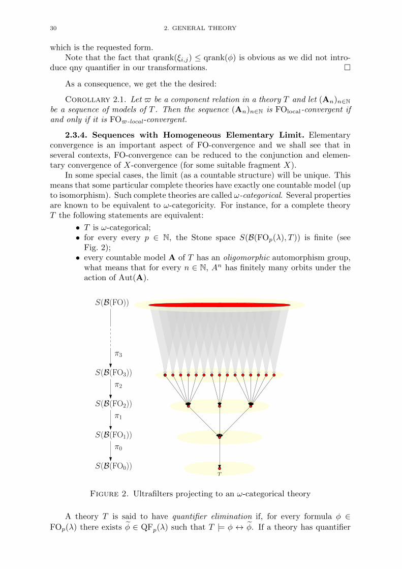
30 2. GENERAL THEORY
which is the requested form.Note that the fact that qrank(ξi,j) ≤ qrank(φ) is obvious as we did not intro-
duce qny quantifier in our transformations.
As a consequence, we get the the desired:
Corollary 2.1. Let $ be a component relation in a theory T and let (An)n∈Nbe a sequence of models of T . Then the sequence (An)n∈N is FOlocal-convergent ifand only if it is FO$-local-convergent.
2.3.4. Sequences with Homogeneous Elementary Limit. Elementaryconvergence is an important aspect of FO-convergence and we shall see that inseveral contexts, FO-convergence can be reduced to the conjunction and elemen-tary convergence of X-convergence (for some suitable fragment X).
In some special cases, the limit (as a countable structure) will be unique. Thismeans that some particular complete theories have exactly one countable model (upto isomorphism). Such complete theories are called ω-categorical. Several propertiesare known to be equivalent to ω-categoricity. For instance, for a complete theoryT the following statements are equivalent:
• T is ω-categorical;• for every every p ∈ N, the Stone space S(B(FOp(λ), T )) is finite (see
Fig. 2);• every countable model A of T has an oligomorphic automorphism group,
what means that for every n ∈ N, An has finitely many orbits under theaction of Aut(A).
S(B(FO0))T
S(B(FO1))
S(B(FO2))
S(B(FO3))
S(B(FO))
π2
π1
π0
π3
Figure 2. Ultrafilters projecting to an ω-categorical theory
A theory T is said to have quantifier elimination if, for every formula φ ∈FOp(λ) there exists φ ∈ QFp(λ) such that T |= φ ↔ φ. If a theory has quantifier
2.3. COMBINING FRAGMENTS 31
elimination then it is ω-categorical. Indeed, for every p, there exists only finitelymany quantifier free formulas with p free variables hence (up to equivalence moduloT ) only finitely many formulas with p free variables. The unique countable model ofa complete theory T with quantifier elimination is ultra-homogeneous, what meansthat every partial isomorphism of finite induced substructures extends as a fullautomorphism. In the context of relational structures, the property of having acountable ultra-homogeneous model is equivalent to the property of having quanti-fier elimination. We provide a proof of this folklore result (in the context of graphs)in order to illustrate these notions.
Lemma 2.24. Let T be a complete theory (of graphs) with no finite model.Then T has quantifier elimination if and only if some (equivalently, every)
countable model of T is ultra-homogeneous.
Proof. Assume that T has an ultra-homogeneous countable model G. Let(a1, . . . , ap), (b1, . . . , bp) be p-tuples of vertices of G. Assume that ai 7→ bi isan isomorphism between G[a1, . . . , ap] and G[b1, . . . , bp]. Then, as G is ultra-homogeneous, there exists an automorphism f of G such that f(ai) = bi for every1 ≤ i ≤ p. As the satisfaction of a first-order formula is invariant by the action ofthe automorphism group, for every formula φ ∈ FOp it holds
G |= φ(a1, . . . , ap) ⇐⇒ G |= φ(b1, . . . , bp).
Consider a maximal set F of p-tuples (v1, . . . , vp) of G such that G |= φ(v1, . . . , vp)and no two p-tuples induce isomorphic (ordered) induced subgraphs. Obviously
|F| = 2O(p2) is finite. Moreover, each p-tuple ~v = (v1, . . . , vp) defines a quantifierfree formula η~v with p free variables such that G |= η~v(x1, . . . , xp) if and only ifxi 7→ vi is an isomorphism between G[x1, . . . , xp] and G[v1, . . . , vp]. Hence it holds:
G |= φ↔∨
~v∈Fη~v.
In other words, φ is equivalent (modulo T ) to the quantifier free formula φ =∨~v∈F η~v, that is: T has quantifier elimination.
Conversely, assume that T has quantifier elimination. As notice above, T is ω-categorical thus has a unique countable model. Assume (a1, . . . , ap) and (b1, . . . , bp)are p-tuples of vertices such that f : ai 7→ bi is a partial isomorphism. Assumethat f does not extend into an automorphism of G. Let (a1, . . . , aq) be a tupleof vertices of G of maximal length such that there exists bp+1, . . . , bq such thatai 7→ bi is a partial isomorphism. Let aq+1 be a vertex distinct from a1, . . . , aq. Letφ(x1, . . . , xq) be the formula
∧
ai∼aj(xi ∼ xj) ∧
∧
¬(ai∼aj)¬(xi ∼ xj) ∧
∧
1≤i≤q¬(xi = xj)
∧ (∃y)
( ∧
ai∼aq+1
(xi ∼ y) ∧∧
¬(ai∼aq+1)
¬(xi ∼ y) ∧∧
1≤i≤q¬(xi = y)
)
As T has quantifier elimination, there exists a quantifier free formula φ such that
T |= φ ↔ φ. As G |= φ(a1, . . . , aq) (witnessed by aq+1) it holds G |= φ(a1, . . . , aq)
hence G |= φ(b1, . . . , bq) (as ai 7→ bi, 1 ≤ i ≤ q is a partial isomorphism) thusG |= φ(b1, . . . , bq). It follows that there exists bq+1 such that ai 7→ bi, 1 ≤ i ≤ q + 1is a partial isomorphism, contradicting the maximality of (a1, . . . , aq).
32 2. GENERAL THEORY
When a sequence of graphs is elementarily convergent to an ultra-homogeneousgraph (i.e. to a complete theory with quantifier elimination), we shall prove thatFO-convergence reduces to QF-convergence. This later mode of convergence is ofparticular interest as it is equivalent to L-convergence.
Lemma 2.25. Let (Gn)n∈N be sequence of graphs that converges elementarily
to some ultra-homogeneous graph G. Then the following properties are equivalent:
• the sequence (Gn)n∈N is FO-convergent;• the sequence (Gn)n∈N is QF-convergent.• the sequence (Gn)n∈N is L-convergent.
Proof. As FO-convergence implies QF-convergence we only have to prove theopposite direction. Assume that the sequence (Gn)n∈N is QF-convergent. Accord-ing to Lemma 2.24, for every formula φ ∈ FOp there exists a quantifier free formula
φ ∈ QFp such that G |= φ↔ φ (i.e. Th(G) has quantifier elimination). As G is anelementary limit of the sequence (Gn)n∈N there exists N such that for every n ≥ Nit holds Gn |= φ ↔ φ. It follows that for every n ≥ N it holds 〈φ,Gn〉 = 〈φ, Gn〉hence limn→∞〈φ,Gn〉 exists. Thus the sequence (Gn)n∈N is FO-convergent.
There are not so many countable ultra-homogeneous graphs.
Theorem 2.26 (Lachlan and Woodrow [47]). Every infinite countable ultraho-mogeneous undirected graph is isomorphic to one of the following:
• the disjoint union of m complete graphs of size n, where m,n ≤ ω and atleast one of m or n is ω, (or the complement of it);
• the generic graph for the class of all countable graphs not containing Kn
for a given n ≥ 3 (or the complement of it).• the Rado graph R (the generic graph for the class of all countable graphs).
Among them, the Rado graph R (also called “the random graph”) is charac-terized by the extension property: for every finite disjoint subsets of vertices A andB of R there exists a vertex z of R−A−B such that z is adjacent to every vertexin A and to no vertex in B. We deduce for instance the following application ofLemma 2.25.
Example 2.27. It is known [9, 10] that for every fixed k, Paley graphs ofsufficiently large order satisfy the k-extension property hence the sequence of Paleygraphs converge elementarily to the Rado graph. Moreover, Paley graphs is astandard example of quasi-random graphs [19], and the sequence of Paley graphsis L-convergent to the 1/2-graphon. Thus, according to Lemma 2.25, the sequenceof Paley graphs is FO-convergent.
We now relate more precisely the extension property with quantifier elimina-tion.
Definition 2.28. Let k ∈ N. A graph G has the k-extension property if, forevery disjoint subsets of vertices A,B of G with size k there exists a vertex z not inA∪B that is adjacent to every vertex in A and to no vertex in B. In other words,
2.3. COMBINING FRAGMENTS 33
G has the k-extension property if G satisfies the sentence Υk below:
(∀x1, . . . , x2k)
( ∧
1≤i<j≤2k
¬(xi = xj)
→ (∃z)2k∧
i=1
¬(xi = z) ∧k∧
i=1
(xi ∼ z) ∧2k∧
i=k+1
¬(xi ∼ z))
Lemma 2.29. Let G be a graph and let p, r be integers.If G has the (p+r)-extension property then every formula φ with p free variables
and quantifier rank r is equivalent, in G, with a quantifier free formula.
Proof. Let φ be a formula with p free variables and quantifier rank r. Let(a1, . . . , ap) and (b1, . . . , bp) be two p-tuples of vertices of G such that ai 7→ bi is apartial isomorphism. The (p+r)-extension properties allows to easily play a r-turnsback-and-forth game between (G, a1, . . . , ap) and (G, b1, . . . , bp), thus proving that(G, a1, . . . , ap) and (G, b1, . . . , bp) are r-equivalent. It follows thatG |= φ(a1, . . . , ap)if and only if G |= φ(b1, . . . , bp). Following the lines of Lemma 2.24, we deduce that
there exists a quantifier free formula φ such that G |= φ↔ φ.
We now prove that random graphs converge elmentarily to the countable ran-dom graphs.
Lemma 2.30. Let 1/2 > δ > 0. Assume that for every positive integer n ≥ 2and every 1 ≤ i < j ≤ n, pn,i,j ∈ [δ, 1 − δ]. Assume that for each n ∈ N, Gn isa random graph on [f(n)] where f(n) ≥ n, and where i and j are adjacent withprobability pn,i,j (all these events being independent). Then the sequence (Gn)n∈Nalmost surely converges elementarily to the Rado graph.
Proof. Let p ∈ N and let α = δ(1 − δ). The probability that Gn |= Υp is at
least 1− (1− αp)f(n). It follows that for N ∈ N the probability that all the graphsGn (n ≥ N) satisfy Υp is at least 1−α−p(1−αp)f(N). According to Borel-Cantellilemma, the probability that Gn does not satisfy Υp infinitely many is zero. As thisholds for every integer p, it follows that, with high probability, every elementarilyconverging subsequence of (Gn)n∈N converges to the Rado graph hence, with highprobability, (Gn)n∈N converges elementarily to the Rado graph.
Thus we get:
Theorem 2.31. Let 0 < p < 1 and let Gn ∈ G(n, p) be independent randomgraphs with edge probability p. Then (Gn)n∈N is almost surely FO-convergent.
Proof. This is an immediate consequence of Lemma 2.25, Lemma 2.30 andthe easy fact that (Gn)n∈N is almost surely QF-convergent.
Theorem 2.32. For every φ ∈ FOp there exists a polynomial Pφ ∈Z[X1, . . . , X(p2)
] such that for every sequence (Gn)n∈N of finite graphs that converges
elementarily to the Rado graph the following holds:If (Gn)n∈N is L-convergent to some graphon W then
limn→∞
〈φ,Gn〉 =
∫· · ·∫Pφ((Wi,j(xi, xj))1≤i<j≤p) dx1 . . . dxp.

34 2. GENERAL THEORY
Proof. Assume the sequence (Gn)n∈N is elementarily convergent to the Radograph and that it is L-convergent to some graphon W .
According to Lemma 2.24, there exists a quantifier free formula φ such that
G |= (∀x1 . . . xp) φ(x1, . . . , xp)↔ φ(x1, . . . , xp)
(hence Ωφ(G) = Ωφ(G)) holds when G is the Rado graph. As (Gn)n∈N is elemen-
tarily convergent to the Rado graph, this sentence holds for all but finitely many
graphs Gn. Thus for all but finitely many Gn it holds 〈φ,Gn〉 = 〈φ, Gn〉. Moreover,according to Lemma 2.25, the sequence (Gn)n∈N is FO-convergent and thus it holds
limn→∞
〈φ,Gn〉 = limn→∞
〈φ, Gn〉.
By using inclusion/exclusion argument and the general form of the density ofhomomorphisms of fixed target graphs to a graphon we deduce that there exists apolynomial Pφ ∈ Z[X1, . . . , X(p2)
] (which depends only on φ) such that
limn→∞
〈φ, Gn〉 =
∫· · ·∫Pφ((Wi,j(xi, xj))1≤i<j≤p) dx1 . . . dxp.
The theorem follows.
Although elementary convergence to Rado graph seems quite a natural assump-tion for graphs which are neither too sparse nor too dense, elementary convergenceto other ultra-homogeneous graphs may be problematic.
Example 2.33. Cherlin [18] posed the problem whether there is a finite k-saturated triangle-free graph, for each k ∈ N, where a triangle free graph is calledk-saturated if for every set S of at most k vertices, and for every independent subsetT of S, there exists a vertex adjacent to each vertex of T and to no vertex of S−T .In other words, Cherlin asks whether the generic countable triangle-free graph hasthe finite model property, that is if it is an elementary limit of a sequence of finitegraphs.
It is possible to extend Lemma 2.25 to sequences of graph having a non ultra-homogeneous elementary limit if we restrict FO to a smaller fragment. An exampleis the following:
Example 2.34. A graph G is IH-Homogeneous [15] if every partial finite iso-morphism extends into an endomorphism. Let PP be the fragment of FO thatconsists into primitive positive formulas, that is formulas formed using adjacency,equality, conjunctions and existential quantification only, and let BA(PP ) be theminimum sub-Boolean algebra of FO containing PP.
Following the lines of Lemma 2.25 and using Theorem 2.13 and Proposition 2.1,one proves that if a sequence of graphs (Gn)n∈N converges elementarily to some IH-homogeneous infinite countable graph then (Gn)n∈N is BA(PP)-convergent if andonly if it is QF-convergent.
2.4. INTERPRETATION SCHEMES 35
2.3.5. FO-convergence of Graphs with Bounded Maximum Degree.We now consider how full FO-convergence differs to BS-convergence for sequence ofgraphs with maximum degree at most D. As a corollary of Theorems 2.21 and 2.15we have:
Theorem 2.35. A sequence (Gn) of finite graphs with maximum degree atmost d such that limn→∞ |Gn| = ∞ is FO-convergent if and only if it is both BS-convergent and elementarily convergent.
2.4. Interpretation Schemes
In the process of this research we discovered the increasing role played byinterpretations. They are described in this section.
2.4.1. Continuous Functions and Interpretations. Let X and Y be frag-ments of FO(κ) and FO(λ), respectively. Let f : S(B(X)) → S(B(Y )). Then f iscontinuous if and only if for every X-convergent sequence (An)n∈N, the sequence(f(An))n∈N is Y -convergent. However, relying on the topological definition of con-tinuity, a function f : S(B(X)) → S(B(Y )) is continuous if and only if the inverseimage of an open subset of S(B(Y )) is an open subset of S(B(X)). In the caseof Stone spaces (where clopen subsets generates the topology), we can further re-strict our attention to clopen subsets: f will be continuous if the inverse image ofa clopen subset is a clopen subset. In other words, f is continuous if there existsf∗ : B(Y )→ B(X), such that for every φ ∈ Y , it holds
f−1(K(φ)) = K(f∗(φ)).
Note that f∗ will be a homomorphism from B(Y ) to B(X), and that the dualitybetween f and f∗ is nothing more the duality between Stone spaces and Booleanalgebras.
The above property can be sometimes restated in terms of definable sets instructures. For a fragment X of FO and a relational structure A, a subset F ⊆ Apis X-definable if there exists a formula φ ∈ X with free variables x1, . . . , xp suchthat
F = Ωφ(A) = (v1, . . . , vp) ∈ Ap : A |= φ(v1, . . . , vp).Let A be a κ-structure, let B be a λ-structure, and let g : Ak → B be surjective.
Assume that there exists a function g∗ : Y → X such that for every φ ∈ Y withfree variables x1, . . . , xp (p ≥ 0), and every vi,j ∈ A (1 ≤ i ≤ p, 1 ≤ j ≤ k) it holds
B |= φ(g(v1,1, . . . , v1,k), . . . , g(vp,1, . . . , vp,k))
⇐⇒A |= g∗(φ)(v1,1, . . . , v1,k, . . . , vp,1, . . . , vp,k)
then g∗ is a homomorphism, and thus it defines a continous function fromS(B(X)) to S(B(Y )). Note that the above formula can be restated as
Ωg∗(φ)(A) = g−1(Ωφ(B)),
where
g((v1,1, . . . , vp,k)) = (g(v1,1, . . . , v1,k), . . . , g(vp,1, . . . , vp,k)).

36 2. GENERAL THEORY
In other words, the inverse image of a Y -definable set of B is an X-definable set ofA.
When X = FO(κ) and Y = FO(λ), the property that the inverse image of afirst-order definable set of B is a first-order definable set of A leads to the modeltheoretical notion of interpretation (without parameters) of B in A. We recall nowthe formal definition of an interpretation.
Definition 2.36 (Interpretation). An interpretation of B in A with parameters(or without parameters, respectively) with exponent k is a surjective map from asubset of Ak onto B such that the inverse image of every set X definable in B bya first-order formula without parameters is definable in A by a first-order formulawith parameters (or without parameters, respectively).
2.4.2. Interpretation Schemes. The main drawback of interpretations isthat it only concerns two specific structures A and B. However, it is frequent thatintepretations naturally generalize to a familly of interpretations of λ-structures inκ-structures with the same associated homomorphism of Boolean algebras. More-over, this homomorphism is uniquely defined by the way it transforms each relationin λ (including equality) into a formula in κ and by the formula which defines thedomain of the κ-structures. This can be formalized as follows.
Definition 2.37 (Interpretation Scheme). Let κ, λ be signatures, where λ hasq relational symbols R1, . . . , Rq with respective arities r1, . . . , rq.
An interpretation scheme I of λ-structures in κ-structures is defined by aninteger k — the exponent of the intrepretation scheme — a formula E ∈ FO2k(κ),a formula θ0 ∈ FOk(κ), and a formula θi ∈ FOrik(κ) for each symbol Ri ∈ λ, suchthat:
• the formula E defines an equivalence relation of k-tuples;• each formula θi is compatible with E, in the sense that for every 0 ≤ i ≤ q
it holds∧
1≤j≤riE(xj ,yj) ` θi(x1, . . . ,xri)↔ θi(y1, . . . ,yri),
where r0 = 1, boldface xj and yj represent k-tuples of free variables, andwhere θi(x1, . . . ,xri) stands for θi(x1,1, . . . , x1,k, . . . , xri,1, . . . , xri,k).
For a κ-structure A, we denote by I(A) the λ-structure B defined as follows:
• the domain B of B is the subset of the E-equivalence classes [x] ⊆ Ak ofthe tuples x = (x1, . . . , xk) such that A |= θ0(x);
• for each 1 ≤ i ≤ q and every v1, . . . ,vsi ∈ Akri such that A |= θ0(vj) (forevery 1 ≤ j ≤ ri) it holds
B |= Ri([v1], . . . , [vri ]) ⇐⇒ A |= θi(v1, . . . ,vri).
¿From the standard properties of model theoretical interpretations (see, forinstance [48] p. 180), we state the following: if I is an interpretation of λ-structures
in κ-structures, then there exists a mapping I : FO(λ)→ FO(κ) (defined by meansof the formulas E, θ0, . . . , θq above) such that for every φ ∈ FOp(λ), and everyκ-structure A, the following property holds (while letting B = I(A) and identifyingelements of B with the corresponding equivalence classes of Ak):
For every [v1], . . . , [vp] ∈ Bp (where vi = (vi,1, . . . , vi,k) ∈ Ak) it holds
B |= φ([v1], . . . , [vp]) ⇐⇒ A |= I(φ)(v1, . . . ,vp).

2.4. INTERPRETATION SCHEMES 37
It directly follows from the existence of the mapping I that an interpretation schemeI of λ-structures in κ-structures defines a continuous mapping from S(B(FO(κ)))to S(B(FO(λ))). Thus, interpretation schemes have the following general property:
Proposition 2.3. Let I be an interpretation scheme of λ-structures in κ-structures.
Then, if a sequence (An)n∈N of finite κ-structures is FO-convergent then thesequence (I(An))n∈N of (finite) λ-structures is FO-convergent.
We shall be mostly interested in very specific and simple types of interpretationschemes.
Definition 2.38. Let κ, λ be signatures. A basic interpretation scheme I ofλ-structures in κ-structures with exponent k is defined by a formula θi ∈ FOkri(κ)for each symbol Ri ∈ λ with arity ri.
For a κ-structure A, we denote by I(A) the structure with domain Ak suchthat, for every Ri ∈ λ with arity ri and every v1, . . . ,vri ∈ Ak it holds
I(A) |= Ri(v1, . . . ,vri) ⇐⇒ A |= θi(v1, . . . ,vri).
It is immediate that every basic interpretation scheme I defines a mappingI : FO(λ)→ FO(κ) such that for every κ-structure A, every φ ∈ FOp(λ), and everyv1, . . . ,vp ∈ Ak it holds
I(A) |= φ(v1, . . . ,vp) ⇐⇒ A |= I(φ)(v1, . . . ,vp)
andqrank(I(φ)) ≤ k(qrank(φ) + max
iqrank(θi)).
It follows that for every κ-structure A, every φ ∈ FOp(λ), it holds
Ωφ(I(A)) = ΩI(φ)(A).
In particular, if A is a finite structure, it holds
〈φ, I(A)〉 = 〈I(φ),A〉.


CHAPTER 3
Modelings for Sparse Structures
3.1. Relational Samples Spaces
The notion of relational sample space is a strenghtening of the one of relationalstructure, where it is required that the domain shall be endowed with a suitablestructure of (nice) measurable space.
3.1.1. Definition and Basic Properties.
Definition 3.1. Let λ be a signature. A λ-relational sample space is a λ-structure A, whose domain A is a standard Borel space with the property thatevery first-order definable subset of Ap is measurable. Precisely, for every integerp, and every φ ∈ FOp(λ), denoting
Ωφ(A) = (v1, . . . , vp) ∈ Ap : A |= φ(v1, . . . , vp),it holds Ωφ(A) ∈ ΣpA, where ΣA is the Borel σ-algebra of A.
Note, that in the case of graphs, every relational sample space is a Borel graph(that is a graph whose vertex set is a standard Borel space and whose edge set isBorel), but the converse is not true.
Lemma 3.2. Let λ be a signature, let A be a λ-structure, whose domain A is astandard Borel space with σ-algebra ΣA.
Then the following conditions are equivalent:
(a) A is a λ-relational sample space;(b) for every integer p ≥ 0 and every φ ∈ FOp(λ), it holds Ωφ(A) ∈ ΣpA;
(c) for every integer p ≥ 1 and every φ ∈ FOlocalp (λ), it holds Ωφ(A) ∈ ΣpA;
(d) for every integers p, q ≥ 0, every φ ∈ FOp+q(λ), and every a1, . . . , aq ∈ Aq theset
(v1, . . . , vp) ∈ Ap : A |= φ(a1, . . . , aq, v1, . . . , vp)belongs to ΣpA.
Proof. Items (a) and (b) are equivalent by definition. Also we obviously havethe implications (d) ⇒ (b) ⇒ (c). That (c) ⇒ (b) is a direct consequence ofGaifman locality theorem, and the implication (b)⇒ (d) is a direct consequence ofFubini-Tonelli theorem.
Lemma 3.3. Let A be a relational sample space, let a ∈ A, and let Aa be theconnected component of A containing a.
Then Aa has a measurable domain and, equipped with the σ-algebra of the Borelsets of A included in Aa, it is a relational sample space.
39
40 3. MODELINGS FOR SPARSE STRUCTURES
Proof. Let φ ∈ FOlocalp and let
X = (v1, . . . , vp) ∈ Apa : Aa |= φ(v1, . . . , vp).As φ is local, there is an integer D such that the satisfaction of φ only depends onthe D-neighborhoods of the free variables.
For every integer n ∈ N, denote by B(A, a, n) the substructure of A induced byall vertices at distance at most n from a. By the locality of φ, for every v1, . . . , vpat distance at most n from a it holds
Aa |= φ(v1, . . . , vp) ⇐⇒ B(A, a, n+D) |= φ(v1, . . . , vp).
However, it is easily checked that there is a local first-order formula ϕn ∈ FOlocalp+1
such that for every v1, . . . , vp it holds
B(A, a, n+D) |= φ(v1, . . . , vp)∧p∧
i=1
dist(a, vi) ≤ n ⇐⇒ A |= ϕn(a, v1, . . . , vp).
By Lemma 3.2, it follows that the set Xn = (v1, . . . , vn) ∈ A : A |=ϕn(a, v1, . . . , vp) is measurable. As X =
⋃n∈NXn, we deduce that X is mea-
surable (with respect to ΣpA. In particular, Aa is a Borel subset of A hence Aa,equipped with the σ-algebra ΣAa
of the Borel sets of A included in Aa, is a stan-dard Borel set. Moreover, it is immediate that a subset of Apa belongs to ΣpAa
if and
only if it belongs to ΣpA. Hence, every subset of Apa defined by a local formula ismeasurable with respect to ΣpAa
. By Lemma 3.2, it follows that Aa is a relationalsample space.
3.1.2. Interpretions of Relational Sample Spaces. An elementary inter-pretation with parameter consits in distinguishing a single element, the parameter,by adding a new unary symbol to the signature (e.g. representing a root).
Lemma 3.4. Let A be a λ-relational sample space, let λ+ be the signatureobtained from λ by adding a new unary symbol M and let A+ be obtained fromA by marking a single a ∈ A (i.e. a is the only element x of A+ = A such thatA+ |= M(x)).
Then A+ is a relational sample space.
Proof. Let φ ∈ FOp(λ+). There exists φ′ ∈ FOp+1(λ) such that for every
x1, . . . , xp ∈ A it holds
A+ |= φ(x1, . . . , xp) ⇐⇒ A |= φ(a, x1, . . . , xp).
According to Lemma 3.2, the set of all (x1, . . . , xp) such that A |= φ(a, x1, . . . , xp)is measurable. It follows that A+ is a relational sample space.
Lemma 3.5. Every injective first-order interpretation (with or without param-eters) of a relational sample space is a relational sample space.
Precisely, if f is an injective first-order interpretation of a λ-structure B in aκ-relational sample space A and if we define
ΣB = X ⊆ B : f−1(X) ∈ ΣkA,then (B,ΣB) is a relational sample space.

3.2. MODELINGS 41
Proof. According to Lemma 3.4, we can first mark all the parameters andreduce to the case were the interpretation has no parameters.
Let D be the domain of f . As B is first-order definable in B, D is first-orderdefinable in A hence D ∈ ΣkA. Then D is a Borel sub-space of Ak. As f is abijection from D to B, we deduce that (B,ΣB) is a standard Borel space.
Moreover, as the inverse image of every first-order definable set of B is first-order definable in A, we deduce that (B,ΣB) is a λ-relational sample space.
3.1.3. Disjoint union. Let Hi be λ-relational sample spaces for i ∈ I ⊆ N.We define the disjoint union
H =∐
i∈IHi
of the Hi’s as the relational structure, which is the disjoint union of the Hi’sendowed with the σ-algebra ΣH = ⋃iXi : Xi ∈ ΣHi
.
Lemma 3.6. Let Hi be λ-relational sample spaces for i ∈ I ⊆ N. Then H =∐i∈I Hi is a λ-relational sample space, in which every Hi is measurable.
Proof. We consider the signature λ+ obtained from λ by adding a new binaryrelation $, and the basic interpretation scheme I1 of λ+-structures in λ-structurescorresponding to the addition of the new relation $ by the formula θ$ = 1. Thismeans that for every λ-structure A it holds I1(A) |= (∀x, y) $(x, y). Let H+
i =I1(Hi).
Let H+ =∐i∈I H+
i . Clearly, ΣH+ = ΣH and (H,ΣH) is a standard Borelspace. Moreover, by construction, each Hi is measurable.
Let φ ∈ FOp(λ). First notice that for every (v1, . . . , vp) ∈ Hp+q (which is also(H+)p+q) it holds Ωφ(H) = Ωφ(H+), that is:
H |= φ(v1, . . . , vp) ⇐⇒ H+ |= φ(v1, . . . , vp).
It follows from Lemma 2.23 that the set Ωφ(H+) may be obtained by Booleanoperations, products, and coordinate permuations from sets defined by $-localformulas (which we introduced in Section 2.3.3). As all these operations preservemeasurability, we can assume that φ is $-local. Then Ωφ(H+) is the union of thesets Ωφ(Hi). All these sets are measurable (as Hi is a modeling) thus their unionis measurable (by construction of ΣH). It follows that H+ is a relational samplespace, and so is H (every first-order definable set of H is first-order definable inH+).
3.2. Modelings
We introduced a notion of limit objects — called modelings — for sequences ofsparse graphs and structures, which is a natural generalization of graphings. Theselimit objects are defined by considering a probability measure on a relational sam-ple space. In this section, we show that the most we can expect is that modelingsare limit objects for sequence of sparse structures, and we conjecture that an un-avoidable qualtitative jump occurs for notions of limit structures, which coincideswith the nowhere dense/somewhere dense fronteer (see Conjecture 1.1).

42 3. MODELINGS FOR SPARSE STRUCTURES
3.2.1. Definition and Basic Properties. Recall Definitions 1.4 and 1.6: aλ-modeling A is a λ-relational sample space equipped with a probability measure(denoted νA), and the Stone pairing of φ ∈ FO(λ) and a λ-modeling A is 〈φ,A〉 =νpA(Ωφ(A)). Notice that it follows (by Fubini’s theorem) that it holds
〈φ,A〉 =
∫
x∈Ap1Ωφ(A)(x) dνpA(x)
=
∫· · ·∫
1Ωφ(A)(x1, . . . , xp) dνA(x1) . . . dνA(xp).
Then, generalizing Definition 1.7, we extend the notion of X-convergence tomodelings:
Definition 3.7 (modeling X-limit). Let X be a fragment of FO(λ).If an X-convergent sequence (An)n∈N of λ-modelings satisfies
(∀φ ∈ X) 〈φ,L〉 = limn→∞
〈φ,An〉
for some λ-modeling L, then we say that L is a modeling X-limit of (An)n∈N.
A λ-modeling A is weakly uniform if all the singletons of A have the same mea-sure. Clearly, every finite λ-structure A can be identified with the weakly uniformmodeling obtained by considering the discrete topology on A. This identificationis clearly consistent with our definition of the Stone pairing of a formula and amodeling.
In the case where a modeling A has an infinite domain, the condition for Ato be weakly uniform is equivalent to the condition for νA to be atomless. Thisproperty is usually fulfilled by modeling X-limits of sequences of finite structures.
Lemma 3.8. Let X be a fragment of FO that includes FO0 and the formula(x1 = x2). Then every modeling X-limit of weakly uniform modelings is weaklyuniform.
Proof. Let φ be the formula (x1 = x2). Notice that for every finite λ-structureA it holds 〈φ,A〉 = 1/|A| and that for every infinite weakly uniform λ-structure itholds 〈φ,A〉 = 0.
Let L be a modeling X-limit of a sequence (An)n∈N. Assume limn→∞ |An| =∞. Assume for contradiction that νL has an atom v (i.e. νL(v) > 0). Then〈φ,L〉 ≥ νL(v)2 > 0, contradicting limn→∞〈φ,An〉 = 0. Hence νL is atomless.
Otherwise, |L| = limn→∞ |An| < ∞ (as L is an elementary limit of (An)n∈N).Let N = |L|. Label v1, . . . , vN the elements of L and let pi = νL(vi). Then
1
N
N∑
i=1
p2i −
( 1
N
N∑
i=1
pi
)2
=〈φ,L〉N
− 1
N2
=limn→∞〈φ,An〉
N− 1
N2
= 0
Thus pi = 1/N for every i = 1, . . . , N .
Corollary 3.1. Every modeling FOlocal2 -limit of finite structures is weakly
uniform.

3.2. MODELINGS 43
Lemma 3.9. Let X be a fragment that includes all quantifier free formulas.Assume L is a modeling X-limit of a sequence (Gn)n∈N of graphs with |Gn| →
∞. Let νL be the completion of the measure νL.Then there is at least one mod 0 isomorphism f : [0, 1]→ (L, νL), and for every
such f the graphon W defined by
W (x, y) = 1Ω(x1∼x2)(L)(f(x), f(y))
(for x, y in the domain of f , and W (x, y) = 0 elsewhere) is as a random-freegraphon L-limit of (Gn)n∈N.
Proof. Considering the formula x1 = x2, we infer that νL is atomless. Thismeasure is also atomless and turns L into a standard probability space. Accordingto the isomorphism theorem, all atomless standard probability spaces are mutuallymod 0 isomorphic hence there is at least one mod 0 isomorphism f : [0, 1]→ (L, νL)([0, 1] is considered with Lebesgue measure).
Fix such a mod 0 isomorphism f , defined on [0, 1] \N1, with value on L \N2
(whereN1 andN2 are nullsets). For every Borel measurable function g : Ln → [0, 1],define gf by gf (x1, . . . , xn) = g(f(x1), . . . , f(xn)) if xi /∈ N1 for every 1 ≤ i ≤ nand gf (x1, . . . , xn) = 0 otherwise. Then it holds
∫
[0,1]ngf (x1, . . . , xn) dx1 . . . dxn =
∫
Lng(v1, . . . , vn) dνL(v1) . . . dνL(vn)
=
∫
Lng(v1, . . . , vn) dνL(v1) . . . dνL(vn).
It follows that for every finite graph F with vertex set 1, . . . , n, denoting φF theformula
∧ij∈E(F )(xi ∼ xj), it holds
t(F,W ) =
∫
[0,1]n
∏
ij∈E(F )
W (xi, xj) dx1 . . . dxn
=
∫
Ln
∏
ij∈E(F )
1Ω(x1∼x2)(L)(vi, vj) dνL(v1) . . . dνL(vn)
=
∫
Ln1ΩφF (L)(v1, . . . , vn) dνL(v1) . . . dνL(vn)
= 〈φF ,L〉= limn→∞
〈φF , Gn〉= limn→∞
t(F,Gn).
Hence W is a graphon L-limit of (Gn)n∈N. As W is 0, 1-valued, it is (by definition)random-free.
We deduce the following limitation of modelings as limit objects.
Corollary 3.2. Let X be a fragment that includes all quantifier free formulas.Assume (Gn)n∈N is an X-convergent sequence of graphs with unbounded order,
which is L-convergent to some non random-free graphon W . Then (Gn)n∈N has nomodeling X-limit.
Let us now give some example stressing that the nullsets of the mod 0 iso-morphism f can be quite large, making L and W look quite different. We give

44 3. MODELINGS FOR SPARSE STRUCTURES
now an example in the more general setting of directed graphs and non-symmetricgraphons.
Example 3.10. Let ~Tn be the transitive tournament of order n, that is thedirected graph on 1, . . . , n defined from the natural linear order <n on 1, . . . , nby i→ j if i < j. This sequence is obviously FO-convergent.
It is not difficult to construct a modeling FO-limit of (~Tn)n∈N: Let
L = 0 × Z+∪ ]0, 1[×Z ∪ 1 × Z−,
with the Borel σ-algebra Σ generated by the product topology of Z (with discretetopology) and R (with usual topology). On L we define a linear order <L by(α, i) <L (β, j) if α < β or (α = β) and (i < j). That (L,Σ) is a relational samplespace follows from the o-minimality of ([0, 1], <). The measure νL can be definedas the product of Lebesgue measure on [0, 1] by any probability measure on Z.For instance, for every B ∈ Σ we let νL(B) = λ(B ∩ ([0, 1] × 0)), where λ isLebesgue measure. It is not difficult to check that L is indeed a modeling FO-limit
of (1, . . . , n, <n) ' ~Tn.In this case, a mod 0 isomorphism f : [0, 1]→ L can be defined by f(x) = (x, 0).
The null set N2, although very large, is clearly a νL-nullset, and the obtained (nonsymmetric) random-free graphon W : [0, 1]× [0, 1]→ [0, 1] is simply defined by
W (x, y) =
1 if x < y
0 otherwise.
Note that W corresponds to [0, 1] with its natural order <. This order is clearly anL-limit of <n (but not an elementary limit, as it is dense although no finite orderis).
In the spirit of Lemma 3.2, we propose the following problems:
Problem 3.1. Let L be a modeling FO-limit of a sequence (An)n∈N of λ-structures, and let v ∈ L. Does there exist a sequence (vn)n∈N such that vn ∈ Anand such that the rooted modeling (L, v) is a modeling FO-limit of the rootedstructures (An, vn)?
Problem 3.2. Let L be a modeling FO-limit of a sequence (An)n∈N of λ-structures. Does there exist f : L→∏
i∈NAn such that for every v1, . . . , vk ∈ L, thek-rooted modeling (L, v1, . . . , vk) is a modeling FO-limit of the k-rooted structures(An, f(v1)n, . . . , f(vk)n)?
3.2.2. Interpretation Schemes applied to Modelings. Basic interpreta-tion schemes will be an efficient tool to handle modelings. Let I be an interpretationscheme I of λ-structures in κ-structures. We have seen that I can be extended to amapping from κ-relational sample space to λ-relational sample space. In the casewhere I is a basic interpretation scheme, we further extend I to a mapping fromκ-modeling to λ-modeling: For a κ-modeling A, the λ-modeling B = I(A) is themodeling on the image relational sample space of A with the probability measureνB = νA. This is formalized as follows:
Lemma 3.11. Let I be a basic interpretation scheme I of λ-structures in κ-structures with exponent k. Extend the definition of I to a mapping of κ-modeling
3.2. MODELINGS 45
to λ-modeling by setting νI(A) = νkA. Then for every κ-modeling A and everyφ ∈ FO(λ) it holds
〈φ, I(A)〉 = 〈I(φ),A〉.Proof. Let A be a κ-modeling. For every φ ∈ FOp(λ) it holds
Ωφ(I(A)) = ΩI(φ)(A)
thus 〈φ, I(A)〉 = νpI(A)(Ωφ(I(A))) = νkpA (ΩI(φ)(A)) = 〈I(φ),A〉.
Remark 3.12. If the basic interpretation scheme I is defined by quantifier-free
formulas only, then it is possible to define I in such a way that for every φ ∈ FO(λ)
it holds qrank(I(φ)) ≤ qrank(φ).
The following strengthening of Proposition 2.3 in the case where we consider abasic interpretation scheme is a clear consequence of Lemma 3.11.
Proposition 3.1. Let I be a basic interpretation scheme of λ-structures inκ-structures.
If L is a modeling FO-limit of a sequence (An)n∈N of κ-modelings then I(L) isa modeling FO-limit of the sequence (I(An))n∈N.
Lemma 3.13. Let p ∈ N be a positive integer, let L be a modeling, and let TppL :
Lp → S(B(FOp(λ))) be the function mapping (v1, . . . , vp) ∈ Lp to the completetheory of (L, v1, . . . , vp) (that is the set of the formulas ϕ ∈ FOp(λ) such thatL |= ϕ(v1, . . . , vp)).
Then TppL is a measurable map from (Lp,ΣpL) to S(B(FOp(λ))) (with its Borel
σ-algebra).Let (An)n∈N be an FOp(λ)-convergent sequence of finite λ-structures, and let µp bethe associated limit measure (as in Theorem 2.6).
Then L is an FOp(λ)-limit modeling of (An)n∈N if and only if µp is the push-forward of the product measure νpL by the measurable map Tpp
L , that is:
TppL ∗(ν
pL) = µp.
Proof. Recall that the clopen sets of S(B(FOp(λ))) are of the form K(φ) forφ ∈ FOp(λ) and that they generate the topology of S(B(FOp(λ))) hence also itsBorel σ-algebra.
That TppL is measurable follows from the fact that for every φ ∈ FOp the
preimage of K(φ), that is TppL
−1(K(φ)) = Ωφ(L), is measurable.Assume that L is an FOp(λ)-limit modeling of (An)n∈N. In order to prove that
TppL ∗(ν
pL) = µp, it is sufficient to check it on sets K(φ):
µp(K(φ)) = limn→∞
〈φ,An〉 = 〈φ,L〉 = νpL( TppL
−1(K(φ))).
Conversely, if TppL ∗(ν
pL) = µp then for every φ ∈ FOp(λ) it holds
〈φ,L〉 = νpL( TppL
−1(K(φ))) = µp(K(φ)) = limn→∞〈φ,An〉,hence L is an FOp(λ)-limit modeling of (An)n∈N.

46 3. MODELINGS FOR SPARSE STRUCTURES
If (X,Σ) is a Borel space with a probability measure ν, it is standard to definethe product σ-algebra Σω on the infinite product space XN, which is generated bycylinder sets of the form
R = f ∈ LN : f(i1) ∈ Ai1 , . . . , f(ik) ∈ Aikfor some k ∈ N and Ai1 , . . . , Aik ∈ Σ. The measure νω of the cylinder R definedabove is then
νω(R) =k∏
j=1
ν(Aij ).
By Kolmogorov’s Extension Theorem, this extends to a unique probability measureon Σω (which we still denote by νω). We summarize this as the following (see alsoFig. 3.2.2).
Theorem 3.14. let L be a modeling, and let TpωL : LN → S(B(FO(λ))) be the
function which assigns to f ∈ LN the point of S(B(FO(λ))) corresponding to theset φ : L |= φ(f(1), . . . , f(p)), where Fv(φ) ⊆ 1, . . . , p.
Then TpωL is a measurable map.
Let (An)n∈N be an FO(λ)-convergent sequence of finite λ-structures, and let µ bethe associated limit measure (see Theorem 2.4).
Then L is an FO(λ)-limit modeling of (An)n∈N if and only if
TpωL ∗(νωL) = µ.
Fig. 3.2.2 visualizes Lemma 3.13 and Theorem 3.14.
L
with νL
Tp1L
L2
with ν2L
oo
Tp2L
S2
. . .oo Lp
with νpL
oo
TppL
Sp
LN
with νωL
TpωL
oo
Sω
S(B(FO0))
with δT
S(B(FO1))
with µ1
oo S(B(FO2))
with µ2
oo
S2
. . .oo S(B(FOp))
with µpoo
Sp
S(B(FO))
with µoo
Sω
S(B(FO1))2
with µ21
``AAAAAAAAAAAS2
. . .oo S(B(FO1))
p
with µp1
oo
Sp
S(B(FO1))
N
with µω1
oo
Sω
Figure 1. Pushforward of measures
Remark 3.15. We could have considered that free variables are indexed by Zinstead of N. In such a context, natural shift operations S and T act respectively onthe Stone space S of the Lindendaum-Tarski algebra of FO(λ), and on the space LZ
of the mappings from Z to a λ-modeling L. If (An)n∈N is an FO-convergent sequencewith limit measure µ on S, then (S, µ, S) is a measure-preserving dynamical system.Also, if νZ is the product measure on A, (AZ, ν, T ) is a Bernoulli scheme. Then, the

3.2. MODELINGS 47
condition of Theorem 3.14 can be restated as follows: the modeling L is a modelingFO-limit of the sequence (An)n∈N if and only if (S, µ, S) is a factor of (AZ, νZ, T ).This setting leads to yet another interpretation of our result, which we hope willbe treated elsewhere.
3.2.3. Component-Local Formulas. The basis observation is that for $-local formulas, we can reduce the Stone pairing to components.
Lemma 3.16. Let A be a λ-modeling and component relation $. Let ψ ∈FOp(λ) be a $-local formula of A.
Assume A has countably many connected components Aii∈Γ. Let Γ+ be theset of indexes i such that νA(Ai) > 0. For i ∈ Γ+ we equip Ai with the σ-algebraΣAi
and the probability measure νAi, where ΣAi
is restriction of ΣA to Ai and, forX ∈ ΣAi
, νAi(X) = νA(X)/νA(Ai). Then
〈ψ,A〉 =∑
i∈Γ
νA(Ai)p 〈ψ,Ai〉.
Proof. First note that each connected component of A is measurable: let Ai
be a connected component of A and let a ∈ Ai. Then Ai = x ∈ A : A |= $(x, a)hence Ai is measurable as A is a relational sample space. Let Y = (v1, . . . , vp) ∈Ap : A |= ψ(v1, . . . , vp). Then 〈ψ,A〉 = νpA(Y ). As ψ is $-local, it also holdsY =
⋃i∈Γ Yi, where Yi = (v1, . . . , vp) : Ai |= ψ(v1, . . . , vp) = Y ∩ Api . As
Ai ∈ ΣA and Y ∈ ΣpA, it follows that Yi ∈ ΣpA and (by countable additivity) itholds
〈ψ,A〉 = νpA(Y ) =∑
i∈Γ
νpA(Yi) =∑
i∈Γ+
νA(Ai)pνpAi
(Yi) =∑
i∈Γ
νA(Ai)p 〈ψ,Ai〉.
Corollary 3.3. Let A be a finite λ-structure with component relation $. Letψ ∈ FOp(λ) be a $-local formula of A.
Let A1, . . . ,An be the connected components of A. Then
〈ψ,A〉 =
n∑
i=1
( |Ai||A|
)p〈ψ,Ai〉.
We are now ready to reduce Stone pairing of local formulas to Stone pairingswith $-local formulas on connected components.
Theorem 3.17. Let p ∈ N and φ ∈ FOlocalp (λ).
Then there exist $-local formulas ξi,j ∈ FOlocalqi,j (1 ≤ i ≤ n, j ∈ Ii) with
qrank(ξi,j) ≤ qrank(φ) such that for each i,∑j∈Ii qi,j = p and, for every modeling
A with component relation $ and countable set of connected components Akk∈Γ,it holds
〈φ,A〉 =n∑
i=1
∏
j∈Ii
∑
k∈Γ
νA(Ak)qi,j 〈ξi,j ,Ak〉.
Proof. This is a direct consequence of Lemmas 2.23 and 3.16.

48 3. MODELINGS FOR SPARSE STRUCTURES
The case of sentences can be handled easily by limited counting. For a set Xand an integer m, define
Bigm(X) =
1 if |X| ≥ m0 otherwise
Lemma 3.18. Let θ ∈ FO0(λ).
Then there exist formulas ψ1, . . . , ψs ∈ FOlocal1 with quantifier rank at most
q(qrank(θ)), integers m1, . . . ,ms ≤ qrank(θ), and a Boolean function F such thatfor every λ-structure A with component relation $ and connected components Bi
(i ∈ I), the property A |= θ is equivalent to
F (Bigm1(i,Bi |= (∃x)ψ1(x)), . . . ,Bigms(i,Bi |= (∃x)ψs(x))) = 1.
Proof. Indeed, it follows from Gaifman locality theorem 2.19 that — in pres-ence of a component relation $ — every sentence θ with quantifier rank r can bewritten as a Boolean combination of sentences θk of the form
∃y1 . . . ∃ymk( ∧
1≤i<j≤mk¬$(yi, yj) ∧
∧
1≤i≤mkψk(yi)
)
where ψk is $-local, mk ≤ qrank(θ), and qrank(ψk) ≤ q(qrank(θ)), for some fixedfunction q. As A |= θk if and only if Bigmk(i,Bi |= (∃x)ψk(x)) = 1, the lemmafollows.
3.2.4. Convex Combinations of Modelings. In several contexts, it is clearwhen disjoint union of converging sequences form a converging sequence. If twograph sequences (Gn)n∈N and (Hn)n∈N are L-convergent or BS-convergent, it isclear that the sequence (Gn ∪Hn)n∈N is also convergent, provided that the limit
limn→∞
|Gn|/(|Gn|+ |Hn|)
exists. The same applies if we merge a countable set of L-convergent (resp. BS-convergent) sequences (Hn,i)n∈N (where i ∈ N), with the obvious restriction thatfor each i ∈ N all but finitely many Hn,i are empty graphs.
We shall see that the possibility to merge a countable set of converging se-quences to FOlocal-convergence will need a further assumption, namely the followingequality:
∑
i
limn→∞
|Gn,i||⋃j Gn,j |
= 1.
The importance of this assumption is illustrated by the next example.
Example 3.19. Let Nn = 22n (so that N(n) is divisible by 2i for every 1 ≤i ≤ 2n). Consider sequences (Hn,i)n∈N of edgeless black and white colored graphswhere Hn,i is
• empty if i > 2n,• the edgeless graph with (2−i + 2−n)Nn white vertices and 2−iNn black
vertices if n is odd,• the edgeless graph with (2−i + 2−n)Nn black vertices and 2−iNn white
vertices if n is even.

3.2. MODELINGS 49
For each i ∈ N, the sequence (Hn,i)n∈N is obviously L-convergent (and even FO-convergent) as the proportion of white vertices in Hn,i tends to 1/2 as n→∞. Theorder of Gn =
⋃i∈NHn,i is 3Nn and |Hn,i|/|Gn| tends to 2
3 .2−i as n goes to infinity.
However the sequence (Gn)n∈N is not L-convergent (hence not FOlocal-convergent).Indeed, the proportion of white vertices in Gn is 2/3 if n is odd and 1/3 is n iseven.
Hence, we are led to the following definition.
Definition 3.20 (Convex combination of Modelings). Let Hi be λ-modelingsfor i ∈ I ⊆ N and let (αi)i∈I be positive real numbers such that
∑i∈I αi = 1.
Let H =∐i∈I Hi be the relational sample space obtained as the disjoint union
of the Hi. We endow H with the probability measure νH(X) =∑i αiνHi(X ∩Hi).
Then H is the convex combination of modelings Hi with weights αi and wedenote it by
∐i∈I(Hi, αi).
Lemma 3.21. Let Hi be λ-modelings for i ∈ I ⊆ N and let (αi)i∈I be positivereal numbers such that
∑i∈I αi = 1. Let H =
∐i∈I(Hi, αi) Then
(1) H is a modeling, each Hi is measurable and νH(Hi) = αi holds for everyi ∈ I;
(2) if all the Hi are weakly uniform and either all the Hi are infinite or allthe Hi are finite, I is finite, and αi = |Hi|/
∑i∈I |Hi|, then H is weakly
uniform.
Proof. According to Lemma 3.2, H is a relational sample space, in whicheach Hi is measurable. That νH(Hi) = αi immediately follows from the definitionof νH.
Assume that all the Hi are weakly uniform. If all the Hi are finite, I is finite,and αi = |Hi|/
∑i∈I |Hi|, then H is the modeling associated to the union of the
Hi hence it is weakly uniform. Otherwise all the Hi are infinite, hence all the νHi
are atomless, νH is atomless, and H is weakly uniform.
Lemma 3.22. Let p ∈ N and φ ∈ FOlocalp (λ).
Then there exist local formulas ξi,j ∈ FOlocalqi,j (1 ≤ i ≤ n, j ∈ Ii) with
qrank(xii,j) ≤ qrank(φ) such that for each i,∑j∈Ii qi,j = p and, for every count-
able set of modelings Ak and weights αk (k ∈ Γ ⊆ N and∑k αk = 1) it holds,
denoting A =∐i∈Γ(Ai, αi):
〈φ,A〉 =
n∑
i=1
∏
j∈Ii
∑
k∈Γ
αqi,jk 〈ξi,j ,Ak〉.
Proof. Considering, as above, the combination A+ =∐i∈Γ(A+
i , αi), where
A+i is obtained by the basic interpretation scheme adding a full binary relation $,
the result is an immediate consequence of Theorem 3.17.
For λ-modelings A and B, and p, r ∈ N define
‖A−B‖localp,r = sup|〈φ,A〉 − 〈φ,B〉| : φ ∈ FOlocal
p (λ), qrank(φ) ≤ r.The following lemma relates precisely how close are Stone pairings on two combina-tions of modelings, when the modelings and weights involved in the combinationsdefine close Stone pairings.

50 3. MODELINGS FOR SPARSE STRUCTURES
Lemma 3.23. Let p, r ∈ N, and let Γ ⊆ N. For k ∈ Γ, let Ak,Bk be λ-modelings, and let αk, βk be non-negative weights with
∑k αk =
∑k βk = 1.
Let A =∐i∈Γ(Ai, αi) and B =
∐i∈Γ(Bi, βi). Then there exists a constant cr,p
(which depends only on λ, r, and p) such that it holds
‖A−B‖localp,r ≤ cr,p
(‖α− β‖1 +
∑
k∈Γ
αk‖Ak −Bk‖localp,r
)
≤ cr,p(‖α− β‖1 + sup
i∈Γ‖Ai −Bi‖local
p,r
).
Proof. Let φ ∈ FOlocalp (λ) with qrank(φ) ≤ r. According to Lemma 3.22
there exist local formulas ξi,j ∈ FOlocalqi,j (λ) (1 ≤ i ≤ n, j ∈ Ii) with qrank(xii,j) ≤ r
such that for each i,∑j∈Ii qi,j = p and, for every countable set of modelings Ck
and weights γk (k ∈ Γ and∑k γk = 1) it holds, denoting C =
∐i∈Γ(Ci, γi):
〈φ,C〉 =n∑
i=1
∏
j∈Ii〈ξi,j ,C〉, with 〈ξi,j ,C〉 =
∑
k∈Γ
γqi,jk 〈ξi,j ,Ck〉.
As there are only finitely many non-equivalent formulas in FOlocalp (λ) with quantifier
rank at most r, there is a constant Nr,p such that n ≤ Nr,p.We have
|〈φ,A〉 − 〈φ,B〉| ≤n∑
i=1
∣∣∣∣∏
j∈Ii〈ξi,j ,A〉 −
∏
j∈Ii〈ξi,j ,B〉
∣∣∣∣
Note that if ai, bi ∈ [0, 1] then we get easily
∣∣∣∣k∏
i=1
ai −k∏
i=1
bi
∣∣∣∣ =
∣∣∣∣(a1 − b1)k∏
i=2
ai + b1( k∏
i=2
ai −k∏
i=2
bi)∣∣∣∣
≤ |a1 − b1|+∣∣∣∣k∏
i=2
ai −k∏
i=2
bi
∣∣∣∣
≤k∑
i=1
|ai − bi|
Hence, as for every 1 ≤ i ≤ n and every j ∈ I it holds 0 ≤ 〈ξi,j ,A〉 ≤ 1 and0 ≤ 〈ξi,j ,B〉 ≤ 1, we have
|〈φ,A〉 − 〈φ,B〉| ≤n∑
i=1
∑
j∈Ii
∣∣∣∣〈ξi,j ,A〉 − 〈ξi,j ,B〉∣∣∣∣
≤n∑
i=1
∑
j∈Ii
∣∣∣∣∑
k∈Γ
αqi,jk 〈ξi,j ,Ak〉 −
∑
k∈Γ
βqi,jk 〈ξi,j ,Bk〉
∣∣∣∣
≤n∑
i=1
∑
j∈Ii
∑
k∈Γ
∣∣αqi,jk 〈ξi,j ,Ak〉 − βqi,jk 〈ξi,j ,Bk〉∣∣

3.2. MODELINGS 51
Thus, as qi,j ≥ 1 and as Stone pairings 〈 · , · 〉 have value in [0, 1], it holds (denotingcr,p = pNr,p):
‖A−B‖localp,r ≤ cr,p
(∑
k∈Γ
|αk − βk|+∑
k∈Γ
αk‖Ak −Bk‖localp,r
)
Lemma 3.24. Let p, r ∈ N, let A,B be λ-modeling, with connected componentsAk, k ∈ ΓA and Bk, k ∈ ΓB (where ΓA and ΓB can be infinite non-countable).
Then it holds
‖A−B‖localp,r < cr,p
(supk∈ΓA
νA(Ak) + supk∈ΓB
νB(Bk) + ‖A−B‖local1,r
).
Proof. Let φ ∈ FOlocalp (λ) with qrank(φ) ≤ r. It holds
〈φ,A〉 =
n∑
i=1
∏
j∈Ii〈ξi,j ,A〉.
It is clear that if ζi,j is component-local and qi,j > 1 then
〈ξi,j ,A〉 < supk∈ΓA
νA(Ak).
Let X be the set of the integers 1 ≤ i ≤ n such that there is j ∈ Ii such thatqi,j > 1, and let Y be the complement of X in 1, . . . , n. Then
∣∣〈φ,A〉 −∑
i∈Y
∏
j∈Ii〈ξi,j ,A〉
∣∣ < cr,p supk∈ΓA
νA(Ak).
Similarly, it holds
∣∣〈φ,B〉 −∑
i∈Y
∏
j∈Ii〈ξi,j ,B〉
∣∣ < cr,p supk∈ΓB
νB(Bk).
Thus the statement follows from∣∣∣∣∑
i∈Y
∏
j∈Ii〈ξi,j ,A〉 −
∑
i∈Y
∏
j∈Ii〈ξi,j ,B〉
∣∣∣∣ ≤∑
i∈Y
∣∣∣∣∏
j∈Ii〈ξi,j ,A〉 −
∏
j∈Ii〈ξi,j ,B〉
∣∣∣∣
≤∑
i∈Y
∑
j∈Ii
∣∣〈ξi,j ,A〉 − 〈ξi,j ,B〉∣∣
≤ cr,p‖A−B‖local1,r
Theorem 3.25. Let p ∈ N, let I ⊆ N and, for each i ∈ I let (Ai,n)n∈N be
an FOlocalp (λ)-convergent sequence of λ-modelings and let (ai,n)n∈N be a convergent
sequence of non-negative real numbers, such that∑i∈I ai,n = 1 holds for every
n ∈ N, and such that∑i∈I limn→∞ ai,n = 1.
Then the sequence of convex combinations∐i∈I(Ai,n, ai,n) is FOlocal
p (λ)-convergent.

52 3. MODELINGS FOR SPARSE STRUCTURES
Proof. If I is finite, then the result follows from Lemma 3.22. Hence we canassume I = N.
Let φ ∈ FOlocalp , let q ∈ N, and let ε > 0 be a positive real. Assume that
for each i ∈ N the sequence (Ai,n)n∈N is FOlocalp -convergent and that (ai,n)n∈N is
a convergent sequence of non-negative real numbers, such that∑i ai,n = 1 holds
for every n ∈ N. Let αi = limn→∞ ai,n, let di = limn→∞〈φ,Ai,n〉, and let C be
such that∑Ci=1 αi > 1 − ε/4. There exists N such that for every n ≥ N and
every i ≤ C it holds |an,i − αi| < ε/4C and |aqi,n〈φ,Ai,n〉 − αqi di| < ε/2C. Thus∣∣∣∑Ci=1 a
qi,n〈φ,Ai,n〉 −
∑Ci=1 α
qi di
∣∣∣ < ε/2 and∑i>C+1 ai,n < ε/2. It follows that for
any n ≥ N it holds∣∣∣∣∣∑
i>C+1
aqi,n〈φ,Ai,n〉 −∑
i>C+1
αqi di
∣∣∣∣∣ ≤ max
( ∑
i>C+1
aqi,n,∑
i>C+1
αqi di
)< ε/2
hence |∑i aqi,n〈φ,Ai,n〉 −
∑i α
qi di| < ε.
For every ψ ∈ FOlocalp , the expression appearing in Lemma 3.22 for the
expansion of 〈φ,∐i(Ai,n, ai,n)〉 is a finite combination of terms of the form∑i aqi,ni,n 〈φ,Ai,n〉, where qi,n ∈ N and φ ∈ FOlocal
p . It follows that the value
〈φ,∐i(Ai,n, ai,n)〉 converges as n grows to infinity. Hence (∐i(Ai,n, ai,n))n∈N is
FOlocalp -convergent.
Corollary 3.4. Let p ≥ 1 and let (An)n∈N be a sequence of finite λ-structures.Assume An be the disjoint union of Bn,i (i ∈ N) where all but a finite number
of Bn,i are empty. Let an,i = |Bn,i|/|An|. Assume further that:
• for each i ∈ N, the limit αi = limn→∞ an,i exists,
• for each i ∈ N such that αi 6= 0, the sequence (Bn,i)n∈N is FOlocalp -
convergent,• it holds ∑
i≥1
αi = 1.
Then, the sequence (An)n∈N is FOlocalp -convergent.
Moreover, if Li is a modeling FOlocalp -limit of (Bn,i)n∈N when αi 6= 0 then∐
i(Li, αi) is a modeling FOlocalp -limit of (An)n∈N.
Proof. This follows from Theorem 3.25, as An =∐i(Bn,i, an,i).
Definition 3.26. A family of sequence (Ai,n)n∈N (i ∈ I) of λ-structures isuniformly elementarily convergent if, for every formula φ ∈ FO1(λ) there is aninteger N such that it holds
∀i ∈ I, ∀n′ ≥ n ≥ N, (Ai,n |= (∃x)φ(x)) =⇒ (Ai,n′ |= (∃x)φ(x)).
First notice that if a family (Ai,n)n∈N (i ∈ I) of sequences is uniformly elemen-tarily convergent, then each sequence (Ai,n)n∈N is elementarily convergent
Lemma 3.27. Let I ⊆ N , and let (Ai,n)n∈N (i ∈ I) be sequences forming auniformly elementarily convergent family.
Then (⋃i∈I Ai,n)n∈N is elementarily convergent.
3.2. MODELINGS 53
Moreover, if (Ai,n)n∈N is elementarily convergent to Ai then (⋃i∈I Ai,n)n∈N
is elementarily convergent to⋃i∈I Ai.
Proof. Let λ+ be the signature λ augmented by a binary relational symbol $.Let I1 be the basic interpretation scheme of λ+-structures in λ-structures defining$(x, y) for every x, y. Let A+
i,n = I1(Ai,n). According to Lemma 3.18, for every
sentence θ ∈ FO0(λ) there exist formulas ψ1, . . . , ψs ∈ FOlocal1 , an integer m, and a
Boolean function F such that the property⋃i∈I A+
i,n |= θ is equivalent to
F (Bigm1(i,Ai,n |= (∃x)ψ1(x)), . . . ,Bigms(i,Ai,n |= (∃x)ψs(x))) = 1.
According to the definition of a uniformly elementarily convergent family there isan integer N such that, for every 1 ≤ j ≤ s, the value Bigmj (i,Ai,n |= (∃x)ψj(x))is a function of n, which is non-decreasing for n ≥ N . It follows that this func-tion admits a limit for every 1 ≤ j ≤ s hence the exists an integer N ′ such thateither
⋃i∈I A+
i,n |= θ holds for every n ≥ N ′ or it holds for no n ≥ N ′. It fol-
lows that (⋃i∈I A+
i,n)n∈N is elementarily convergent. Thus (by means of the basic
interpretation scheme deleting $) (⋃i∈I Ai,n)n∈N is elementarily convergent
If I is finite, it is easily checked that if (Ai,n)n∈N is elementarily convergent to
Ai then (⋃i∈I Ai,n)n∈N is elementarily convergent to
⋃i∈I Ai.
Otherwise, we can assume I = N. Following the same lines, it is easily checked
that (⋃ni=1 Ai)n∈N converges elementarily to (
⋃i∈N Ai)n∈N. For i, n ∈ N, let
Bi,2n = Ai,n and Bi,2n+1 = Ai. As, for each i ∈ N, Ai is an elementary limit of(Ai,n)n∈N it is easily checked that the family of the sequences (Bi,n)n∈N is uniformlyelementarily convergent. It follows that (
⋃i∈N Bi,n)n∈N is elementarily convergent
thus the elementary limit of (⋃i∈I Ai,n)n∈N and (
⋃ni=1 Ai)n∈N are the same, that
is⋃i∈I Ai.
¿From Corollary 3.4 and Lemma 3.27 then follows the next general result.
Corollary 3.5. Let (An)n∈N be a sequence of finite λ-structures.Assume An be the disjoint union of Bn,i (i ∈ N) where all but a finite number
of Bn,i are empty. Let an,i = |Bn,i|/|An|. Assume that:
• for each i ∈ N, the limit αi = limn→∞ an,i exists and it holds∑
i≥1
αi = 1,
• for each i ∈ N such that αi 6= 0, the sequence (Bn,i)n∈N is FOlocal-convergent,
• the family (Bn,i)n∈N (i ∈ N) is uniformly elementarily convergent.
Then, the sequence (An)n∈N is FO-convergent.Moreover, if Li is a modeling FO-limit of (Bn,i)n∈N when αi 6= 0 and an
elementary limit of (Bn,i)n∈N when αi = 0 then∐i(Li, αi) is a modeling FO-limit
of (An)n∈N.
3.2.5. Random-free graphons and Modelings. A graphon is random-freeif it is 0, 1-valued almost everywhere. Moreover, if two graphons represent thesame L-limit of finite graphs, then either they are both random-free or none of them

54 3. MODELINGS FOR SPARSE STRUCTURES
are (see for instance [44]). Several properties of random-free graph limits have beenstudied.
For example, a graph limit Γ is random-free if and only if the random graphG(n,Γ) of order n sampled from Γ has entropy o(n2) [4, 44] (see also [39]).
A sequence of graphs (Gn)n∈N is L-convergent to a random-free graphon if andonly if the sequence (Gn)n∈N is convergent for the stronger metric δ1 [73], wherethe distance δ1(G,H) of graphs G and H with respective vertex sets x1, . . . , xmand y1, . . . , ym is the minimum over all non-negative m × n matrices A = (αi,jwith row sums 1/m and column sums 1/n of
∑(i,j,g,h)∈∆ αi,gαj,h, where ∆ is the
set of quadruples (i, j, g, h) such that either xi, xj ∈ E(G) or yg, yh ∈ E(H)(but not both).
Lovasz and Szegedy [55] defined a graph property (or equivalently a class ofgraphs) C to be random-free if every L-limit of graphs in C is random-free. Theyprove the following:
Theorem 3.28 (Lovasz and Szegedy [55]). A hereditary class C is random-freeif and only if there exists a bipartite graph F with bipartition (V1, V2) such that nograph obtained from F by adding edges within V1 and V2 is in C.
¿From this result, one deduce for instance that the class of m-partite cographsis random-free [17], generalizing the particular cases of threshold graphs [20] and(more general) cographs [43].
Recall that the Vapnik–Chervonenkis dimension (or simply VC-dimension)VC(G) of a graph G is the maximum integer k such that there exists in G dis-joint vertices ui (1 ≤ i ≤ k) and vI (∅ ⊆ I ⊆ 1, . . . , k) such that ui is adjacent tovI exactly if i ∈ I. We now rephrase Lovasz and Szegedy Theorem 3.28 in termsof VC-dimension.
Theorem 3.29. A hereditary class C is random-free if and only if VC(C) <∞,where
VC(C) = supG∈C
VC(G).
Proof. Let Sk be the bipartite graph with vertices ui (1 ≤ i ≤ k) and vI(∅ ⊆ I ⊆ 1, . . . , k) such that ui is adjacent to vI exactly if i ∈ I.
If VC(C) < k then no graph obtained from Sk by adding edges within the ui’sand the vI ’s is in C hence, according to Theorem 3.28, the class C is random-free.
Conversely, if the class C is random-free there exists, according to Theorem 3.28,a bipartite graph F with bipartition (V1, V2) (with |V1| ≤ |V2|) such that no graphobtained from F by adding edges within V1 and V2 is in C. It is easily checked that
F is an induced subgraph of S|V1|+log2 |V2| so VC(C) < |F |2 + log2 |F |.
The VC-dimension of classes of graphs can also be related to the nowheredense/somewhere dense dichotomy. Recall that a class C is somewhere dense ifthere exists an integer p such that for every integer n the p-subdivision of Kn
is a subgraph of a graph in C, and that the class C is nowhere dense, otherwise[65, 69, 71]. This dichotomy can also be characterized in quite a number of differentways, see [71]. Based on Laskowski [49], another characterization has been proved,which relates this dichotomy to VC-dimension:
Theorem 3.30 (Adler and Adler [2]). For a monotone class of graphs C, thefollowing are equivalent:

3.2. MODELINGS 55
(1) For every interpretation scheme I of graphs in graphs, the class I(C) hasbounded VC-dimension;
(2) For every basic interpretation scheme I of graphs in graphs with exponent1, the class I(C) has bounded VC-dimension;
(3) The class C is nowhere-dense.
¿From Theorem 3.28 and 3.30 we deduce the following:
Theorem 3.31. Let C be a monotone class of graphs. Then the following areequivalent:
(1) For every interpretation scheme I of graphs in graphs, the class I(C) israndom-free;
(2) For every basic interpretation scheme I of graphs in graphs with exponent1, the class I(C) is random-free;
(3) The class C is nowhere-dense.
Proof. Obviously, condition (1) implies condition (2). Assume that (2) andassume for contradiction that (3) does not hold. Then, as C is monotone andsomewhere dense, there is an integer p ≥ 1 such that for every graph n, the p-subdivision Subp(Kn) of the complete graph Kn is in C. To every finite graph G weassociate a graph G′ by considering an arbitrary orientation of G and then buildingG′ as shown on the figure bellow.
p
p
G
p
p
x y
x′ y′
︷ ︸︸ ︷(2p+ 1)(|G| − dG(x))− 1
︷ ︸︸ ︷(2p+ 1)(|G| − dG(y))− 1
p︷ ︸︸ ︷ p︷ ︸︸ ︷ p︷ ︸︸ ︷G′
Note that G′ ∈ C as it is obviously a subgraph of the p-subdivision of thecomplete graph of order (2p + 1)|G|2. It is easily checked that there is a basicinterpretation scheme Ip of graphs in graphs with exponent 1 (which definitionsonly depends on p) such that Ip(G
′) = G[(2p+ 1)|G|], where G[(2p+ 1)|G|] denotesthe graph obtained from G by blowing each vertex to an independent set of size(2p+ 1)|G|.
Let (Gi)i∈N be a sequence of graph that is L-convergent to a non random-free
graphon W . As t(F,G) = hom(F,G)|G||F | is invariant by uniform blow-up of the vertices
of G, for every finite graph F it holds
t(F, Ip(G′i)) = t(F,Gi[(2p+ 1)|Gi|]) = t(F,Gi).

56 3. MODELINGS FOR SPARSE STRUCTURES
Hence (Ip(G′i))i∈N is L-convergent to W . Then the condition 2 contradicts the
hypothesis that W is not random-free. It follows (by contradiction) that (2) implies(3).
Assume condition (3) holds, and let I be an interpretation scheme of graphs ingraphs. Then according to Theorem 3.30 the class I(C) has bounded VC-dimension,hence the hereditary closure of I(C) has bounded VC-dimension thus is random-free,whence I(C) is random-free.
We derive the following corollary concerning existence of modeling FO-limits,which completes Corollary 3.2.
Theorem 3.32. Let C be a monotone class.If every FO-convergent sequence of graphs in C has a modeling FO-limit then
C is nowhere dense.
Proof. Let I be a basic interpretation scheme of graphs in graphs, and let(Gi)i∈N be a sequence of graphs in C such that |Gi| is unbounded, and the sequence(I(Gi))i∈N is L-convergent.
By compactness, the sequence (Gi)i∈N has a subsequence (Gni)i∈N that is FO-convergent. Hence, by hypothesis, (Gni)i∈N has a modeling FO-limit L. Accord-ing to Proposition 3.1, the sequence (I(Gni))i∈N has modeling FO-limit I(L). ByLemma 3.9, L defines a random-free graphon W that is the L-limit of (I(Gni))i∈N.Of course, the L-limit of an L-convergent sequence (Gi)i∈N with |Gi| bounded isalso random-free. Hence the class I(C) is random-free. As this conclusion holds forevery basic interpretation scheme I we deduce from Theorem 3.31 that C is nowheredense.
Actually, we conjecture that the converse is true (see Conjecture 1.1).
3.2.6. Modelings FO-limits for Graphs of Bounded Degrees. Nice limitobjects are known for sequence of bounded degree connected graphs, both for BS-convergence (graphing) and for FO0-convergence (countable graphs). It is naturalto ask whether a nice limit object could exist for full FO-convergence. We shallnow give a positive answer to this question. First we take time to comment on theconnectivity assumption. A first impression is that FO-convergence of disconnectedgraphs could be considered component-wise. This is far from being true in general.The contrast between the behaviour of graphs with a first-order definable compo-nent relation (like graphs with bounded diameter components) and of graphs withbounded degree is exemplified by the following example.
Example 3.33. Consider a BS-convergent sequence (Gn)n∈N of planar graphswith bounded degrees such that the limit distribution has an infinite support. Notethat limn→∞ |Gn| = ∞. Then, as planar graphs with bounded degrees form ahyperfinite class of graphs there exists, for every graph Gn and every ε > 0 asubgraph S(Gn, ε) of Gn obtained by deleting at most ε|Gn| of edges, such thatthe connected components of S(Gn, ε) have order at most f(ε). By considering asubsequence Gs(n) we can assume limn→∞ |Gs(n)|/f(1/n) =∞. Then note that thesequences (Gs(n))n∈N and (S(Gs(n), 1/n))n∈N have the same BS-limit. By merging
these sequences, we conclude that there exists an FOlocal convergent sequence of

3.2. MODELINGS 57
graphs with bounded degrees (Hn) such that Hn is connected if n is even and suchthat the number of connected components of Hn for n odd tends to infinity.
Example 3.34. Using Fig. 2, cConsider four sequences (An)n∈N, (Bn)n∈N,(Cn)n∈N,(Dn)n∈N of FO-converging sequences where |An| = |Bn| = |Cn| = |Dn|grows to infinity, and where these sequences have distinct limits.
Consider a sequence (Gn)n∈N defined as follows: for each n, Gn has two con-nected components denoted by Hn,1 and Hn,2 obtained by joining An, Cn andBn, Dn by a path of length n (for n odd), and by joining An, Dn and Bn, Cn bya path of length n (for n even). Then (Gn)n∈N is FO-convergent. However, thereis no choice of a mapping f : N → 1, 2 such that (Hn,f(n)) is FO-convergent (oreven BS-convergent).
An Bn
Cn Dn
An Bn
Cn Dn
Figure 2. An FO-converging sequence with no component selection
This situation is indeed related to the fact that the diameter of the graph Gn inthe sequence tend to infinity as n grows and that the belonging to a same connectedcomponent cannot be defined by a first-order formula. This situation is standardwhen one consider BS-limits of connected graphs with bounded degrees: it is easilychecked that, as a limit of connected graphs, a graphing may have uncountablymany connected components.
Remark 3.35. In the spirit of the construction shown Fig. 2, we can provethat the set of measure µ which are BS-limits of connected graphs with maximumdegree d ≥ 2 and order going to infinity is convex: Assume (Gn)n∈N and (Hn)n∈Nare convergent sequences with limits µ1 and µ2, and let 0 < α < 1. We constructgraph Mn as follows: let cn = min(|Gn|, |Hn|). We consider α|Hn| copies of Gn and(1− α)|Gn| copies of Hn linked by paths of length blog cnc (see Fig. 3). It is easilychecked that the statistics of the neighborhoods of Mn tend to αµ1 + (1− α)µ2.
Let V be a standard Borel space with a measure µ. Suppose that T1, T2, . . . , Tkare measure preserving Borel involutions of X. Then the system
G = (V, T1, T2, . . . , Tk, µ)
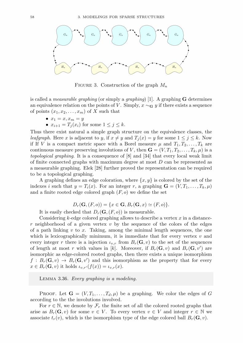
58 3. MODELINGS FOR SPARSE STRUCTURES
Gn Gn Gn Gn Gn
Hn Hn Hn Hn
Figure 3. Construction of the graph Mn
is called a measurable graphing (or simply a graphing) [1]. A graphing G determinesan equivalence relation on the points of V . Simply, x ∼G y if there exists a sequenceof points (x1, x2, . . . , xm) of X such that
• x1 = x, xm = y• xi+1 = Tj(xi) for some 1 ≤ j ≤ k.
Thus there exist natural a simple graph structure on the equivalence classes, theleafgraph. Here x is adjacent to y, if x 6= y and Tj(x) = y for some 1 ≤ j ≤ k. Nowif If V is a compact metric space with a Borel measure µ and T1, T2, . . . , Tk arecontinuous measure preserving involutions of V , then G = (V, T1, T2, . . . , Tk, µ) is atopological graphing. It is a consequence of [8] and [34] that every local weak limitof finite connected graphs with maximum degree at most D can be represented asa measurable graphing. Elek [28] further proved the representation can be requiredto be a topological graphing.
A graphing defines an edge coloration, where x, y is colored by the set of theindexes i such that y = Ti(x). For an integer r, a graphing G = (V, T1, . . . , Tk, µ)and a finite rooted edge colored graph (F, o) we define the set
Dr(G, (F, o)) = x ∈ G, Br(G, x) ' (F, o).It is easily checked that Dr(G, (F, o)) is measurable.Considering k-edge colored graphing allows to describe a vertex x in a distance-
r neighborhood of a given vertex v by the sequence of the colors of the edgesof a path linking v to x. Taking, among the minimal length sequences, the onewhich is lexicographically minimum, it is immediate that for every vertex v andevery integer r there is a injection ιv,r from Br(G, v) to the set of the sequencesof length at most r with values in [k]. Moreover, if Br(G, v) and Br(G, v′) areisomorphic as edge-colored rooted graphs, then there exists a unique isomorphismf : Br(G, v) → Br(G, v′) and this isomorphism as the property that for everyx ∈ Br(G, v) it holds ιv,r′(f(x)) = ιv,r(x).
Lemma 3.36. Every graphing is a modeling.
Proof. Let G = (V, T1, . . . , Td, µ) be a graphing. We color the edges of Gaccording to the the involutions involved.
For r ∈ N, we denote by Fr the finite set of all the colored rooted graphs thatarise as Br(G, v) for some v ∈ V . To every vertex v ∈ V and integer r ∈ N weassociate tr(v), which is the isomorphism type of the edge colored ball Br(G, v).

3.2. MODELINGS 59
According to Gaifman’s locality theorem, in order to prove that G is a model-ing, it is sufficient to prove that for each φ ∈ FOlocal
p , the set
X = (v1, . . . , vp) ∈ V q : G |= φ(v1, . . . , vp)is measurable (with respect to the product σ-algebra of V p).
Let L ∈ N be such that φ is L-local. For every v = (v1, . . . , vp) ∈ X wedefine the graph Γ(v) with vertex set v1, . . . , vp such that two vertices of Γ(v)are adjacent if their distance in G is at most L. We define a partition P(v) of[p] as follows: i and j are in a same part if vi and vj belong to a same connectedcomponent of Γ(v). To each part P ∈ P(v), we associate the tuple formed by TP =t(|P |−1)L(vminP ) and, for each i ∈ P −minP, a composition FP,i = Ti1 · · · Tijwith 1 ≤ j ≤ (|P |−1)L, such that vi = FP,i(vminP ). We also define FP,minP as theidentity mapping. According to the locality of φ, if v′ = (v′1, . . . , v
′p) ∈ V p defines
the same partition, types, and compositions, then v′ ∈ X. For fixed partition P,types (TP )P∈P , and compositions (FP,i)i∈P∈P , the corresponding subset X ′ of Xis included in a (reshuffled) product Y of sets of tuples of the form (FP,i(xminP ))for vminP ∈WP , and is the set of all v ∈ G such that B(|P |−1)L(G, v) = TP . HenceWP is measurable and (as each FP,i is measurable) Y is a measurable subset of
G|P |. Of course, this product may contain tuples v defining another partition. Asimple induction and inclusion/exclusion argument shows that X ′ is measurable.As X is the union of a finite number of such sets, X is measurable.
We now relate graphings to FO-limits of bounded degree graphs. We shallmake use of the following lemma which reduces a graphing to its essential support.
Lemma 3.37 (Cleaning Lemma). Let G = (V, T1, . . . , Td, µ) be a graphing.Then there exists a subset X ⊂ V with 0 measure such that X is globally
invariant by each of the Ti and G′ = (V −X,T1, . . . , Td, µ) is a graphing such thatfor every finite rooted colored graph (F, o) and integer r it holds
µ(Dr(G′, (F, o))) = µ(Dr(G, (F, o)))
(which means that G′ is equivalent to G) and
Dr(G′, (F, o)) 6= ∅ ⇐⇒ µ(Dr(G
′, (F, o))) > 0.
Proof. For a fixed r, define Fr has the set of all (isomorphism typesof) finite rooted k-edge colored graphs (F, o) with radius at most r such thatµ(Dr(G, (F, o))) = 0. Define
X =⋃
r∈N
⋃
(F,o)∈FrDr(G, (F, o)).
Then µ(X) = 0, as it is a countable union of 0-measure sets.We shall now prove that X is a union of connected components of G, and thus
X is globally invariant by each of the Ti. Namely, if x ∈ X and y is adjacentto x, then y ∈ X. Indeed: if x ∈ X then there exists an integer r such thatµ(D(G, Br(G, x))) = 0. But it is easily checked that
µ(D(G, Br+1(G, y))) ≤ d · µ(D(G, Br(G, x))).
Hence y ∈ X. It follows that for every 1 ≤ i ≤ d we have Ti(X) = X. So we candefine the graphing G′ = (V −X,T1, . . . , Td, µ).

60 3. MODELINGS FOR SPARSE STRUCTURES
Let (F, o) be a rooted finite colored graph. Assume there exists x ∈ G′ suchthat Br(G
′, r) ' (F, o). As X is a union of connected components, we also haveBr(G, r) ' (F, o) and x /∈ X. It follows that µ(D(G, (F, o))) > 0 hence it holdsµ(Dr(G
′, (F, o))) > 0.
The cleaning lemma allows us a clean description of FO-limits in the boundeddegree case:
Theorem 3.38. Let (Gn)n∈N be a FO-convergent sequence of finite graphs withmaximum degree d, with limn→∞ |Gn| =∞. Then there exists a graphing G, which
is the disjoint union of a graphing G0 and a countable graph G such that
• The graphing G is a modeling FO-limit of the sequence (Gn)n∈N.• The graphing G0 is a BS-limit of the sequence (Gn)n∈N such that
Dr(G0, (F, o)) 6= ∅ ⇐⇒ µ(Dr(G0, (F, o))) > 0.
• The countable graph G is an elementary limit of the sequence (Gn)n∈N.
Proof. Let G0 be a BS-limit, which has been “cleaned” using the previouslemma, and let G be an elementary limit of G. It is clear that G = G0∪ G is also aBS-limit of the sequence, so the lemma amounts in proving that G is elementarilyequivalent to G.
According to Hanf’s theorem [38], it is sufficient to prove that for every integersr, t and for every rooted finite graph (F, o) (with maximum degree d) the followingequality holds:
min(t, |Dr(G, (F, o))|) = min(t, |Dr(G, (F, o))|).Assume for contradiction that this is not the case. Then |Dr(G, (F, o))| <t and Dr(G0, (F, o)) is not empty. However, as G0 is clean, this impliesµ(Dr(G0, (F, o))) = α > 0. It follows that for every sufficiently large n it holds
|Dr(Gn, (F, o))| > α/2 |Gn| > t. Hence |Dr(G, (F, o))| > t, contradicting our hy-pothesis.
That G is a modeling then follows from Lemma 3.36.
Remark 3.39. Not every graphing with maximum degree 2 is an FO-limitmodeling of a sequence of finite graphs (as it needs not be an elementary limit offinite graphs). Indeed: let G be a graphing that is an FO-limit modeling of thesequence of cycles. The disjoint union of G and a ray is a graphing G′, whichhas the property that all its vertices but one have degree 2, the exceptional vertexhaving degree 1. As this property is not satisfied by any finite graph, G′ is not theFO-limit of a sequence of finite graphs.
Let us finish this section by giving an interesting example, which shows thatthe cleaning lemma sometimes applies in a non-trivial way:
Example 3.40. Consider the graph Gn obtained from a de Bruijn sequence oflength 2n as shown Fig 4.
It is easy to define a graphing G, which is the limit of the sequence (Gn)n∈N: asvertex set, we consider the rectangle [0; 1)× [0; 3). We define a measure preserving

3.2. MODELINGS 61
00
0
0
1
1
1
11
1
1
1
0
0
0
0
Figure 4. The graph Gn is constructed from a de Bruijn sequenceof length 2n.
function f and two measure preserving involutions T1, T2 as follows:
f(x, y) =
(2x, y/2) if x < 1/2 and y < 1
(2x− 1, (y + 1)/2) if 1/2 ≤ x and y < 1
(x, y) otherwise
T1(x, y) =
(x, y + 1) if y < 1
(x, y − 1) if 1 ≤ y < 2
(x, y) otherwise
T2(x, y) =
(x, y + 1) if x < 1/2 and 1 ≤ y < 2
(x, y + 2) if 1/2 ≤ x and y < 1
(x, y − 1) if x < 1/2 and 2 ≤ y(x, y − 2) if 1/2 ≤ x and 2 ≤ y(x, y) otherwise
Then the edges of G are the pairs (x, y), (x′, y′) such that (x, y) 6= (x′, y′)and either (x′, y′) = f(x, y), or (x, y) = f(x′, y′), or (x′, y′) = T1(x, y), or (x′, y′) =T2(x, y).
If one considers a random root (x, y) in G, then the connected componentof (x, y) will almost surely be a rooted line with some decoration, as expectedfrom what is seen from a random root in a sufficiently large Gn. However, specialbehaviour may happen when x and y are rational. Namely, it is possible that theconnected component of (x, y) becomes finite. For instance, if x = 1/(2n − 1) andy = 2n−1x then the orbit of (x, y) under the action of f has length n thus theconnected component of (x, y) in G has order 3n. Of course, such finite connected
62 3. MODELINGS FOR SPARSE STRUCTURES
components do not appear in Gn. Hence, in order to clean G, infinitely manycomponents have to be removed.
Let us give a simple example exemplifying the distinction between BS andFO-convergence for graphs with bounded degree.
Example 3.41. Let Gn denote the n× n grid. The BS-limit object is a prob-ability distribution concentrated on the infinite grid with a specified root. A limitgraphing can be described as the Lebesgue measure on [0, 1]2, where (x, y) is adja-cent to (x± α mod 1, y ± α mod 1) for some irrational number α.
This graphing, however, is not an FO-limit of the sequence (Gn)n∈N as everyFO-limit has to contain four vertices of degree 2. An FO-limit graphing can bedescribed as the above graphing restricted to [0, 1)2 (obtained by deleting all verticeswith x = 1 or y = 1). One checks for instance that this graphing contains fourvertices of degree 2 (the vertices (α, α), (1 − α, α), (α, 1 − α), and (1 − α, 1 − α))and infinitely many vertices of degree 3.
We want to stress that our general and unifying approach to structural limitswas not developed for its own sake and that it provided a proper setting (and,yes, encouragement) for the study of classes of sparse graphs. So far the boundeddegree graphs are the only sparse class of graphs where the structural limits wereconstructed efficiently. (Another example of limits of sparse graphs is provided byscaling limits of transitive graphs [7] which proceeds in different direction and isnot considered here.) The goal of the remaining sections of this article is to extendthis to strong Borel FO-limits of rooted trees with bounded height and thus, bymeans of a fitting basic interpretation scheme, to graphs with bounded tree-depth(defined in [59]), or graphs with bounded SC-depth (defined in [36]).
3.3. Decomposing Sequences: the Comb Structure
The combinatorics of limits of equivalence relations (such as components) iscomplicated. We start this analysis by considering the combinatorics of “large”equivalence classes. This leads to the notion of spectrum, which will be analyzedin this section.
3.3.1. Spectrum of a First-order Equivalence Relation.
Definition 3.42 ($-spectrum). Let A be a λ-modeling (with measure νA),and let $ ∈ FO2(λ) be a formula expressing a component relation on A (seeDefinition 2.22). Let Ci : i ∈ Γ be the set of all the $-equivalence classes ofA, and let Γ+ be the (at most countable) subset of Γ of the indexes i such thatνA(Ci) > 0.
The $-spectrum Sp$(A) of A is the (at most countable) sequence of the valuesνpA(Ci) (for i ∈ Γ+) ordered in non-increasing order.
Lemma 3.43. For k ∈ N, let $(k) be the formula∧ki=1$(xi, xi+1). Then it
holds
∑
i∈Γ+
νA(Ci)k+1 = 〈$(k),A〉.

3.3. DECOMPOSING SEQUENCES: THE COMB STRUCTURE 63
Proof. Let k ∈ N. Define
Dk+1 = (x1, . . . , xk+1) ∈ Ak+1 : A |= $k(x1, . . . , xk+1).According to Lemma 3.3, each Ci is measurable, thus
⋃i∈Γ+
Ci is measurable
and so is R = A \⋃i∈Γ+Ci.
Considering the indicator function 1Dk+1∩Rk+1 of Dk+1 ∩ Rk+1 and applyingFubini’s theorem, we get∫
Ak+1
1Dk+1∩Rk+1 dνk+1A =
∫· · ·∫
1R(x1, . . . , xk+1) dνA(x1, . . . ,dνA(xk+1) = 0.
as for every fixed a1, . . . , ak (with a1 ∈ Cα, for some α ∈ Γ \ Γ+) we have
0 ≤∫
1R(a1, . . . , ak, xk+1) dνA(xk+1) ≤ νA(Cα) = 0.
It follows (by countable additivity) that
〈$(k),A〉 = νk+1A (Dk+1) = νk+1
A (⋃
i∈Γ+
Ck+1i ) =
∑
i∈Γ+
νA(Ci)k+1.
It follows from Lemma 3.43 that the spectrum Sp$(A) is computable from thesequence of (non-increasing) values (〈$(k),A〉)k∈N.
We assume that every finite sequence x = (x1, . . . , xn) of positive reals is im-plicitly embedded in an infinite sequence by defining xi = 0 for i > n. Recall theusual `k norms:
‖x‖k =(∑
i
|xi|k)1/k
.
Hence above equations rewrite as
(3.1) ‖Sp$(A)‖k+1 = 〈$(k),A〉1/(k+1)
We shall prove that the spectrum is, in a certain sense, defined by a continuousfunction. We need the following technical lemma.
Lemma 3.44. For each n ∈ N, let an = (an,i)i∈N be a non-increasing sequenceof positive real numbers with bounded sum (i.e ‖an‖1 <∞ for every n ∈ N).
Assume that for every integer k ≥ 1 the limit sk = limn→∞ ‖an‖k exists.Then (an)n∈N converges in the space c0 of all sequences converging to zero (with
norm ‖ · ‖∞).
Proof. We first prove that the sequences converge pointwise, that is that thereexists a sequence x = (xi)i∈N such that for every i ∈ N it holds
xi = limn→∞
an,i.
For every ε > 0, if sk < ε then an,1 < 2ε for all sufficiently large values of n.Thus if sk = 0 for some k, the limit limn→ an,i exists for every i and is null. Thus,we can assume that sk is strictly positive for every k ∈ N.
Fix k ∈ N. There exists N ∈ N such that for every n ≥ N it holds |skk−‖an‖kk| <skk/k. As (an,i)i∈N is a non-increasing sequence of positive real numbers, for everyn 6= N it holds
akn,1 ≤ ‖an‖kk < skk(1 + 1/k)

64 3. MODELINGS FOR SPARSE STRUCTURES
and
ak−1n,1 ≥ ‖an‖kk > skk(1− 1/k)
Hence
log sk +log(1 + 1/k)
k≥ log an,1 ≥
(1 +
1
k − 1
)(log sk +
log(1− 1/k)
k
)
Thus x1 = limn→∞ an,1 exists and x1 = limk→∞ sk. Inductively, we get that foreach i ∈ N, the limit xi = limn→∞ an,i exists and that
xi = limk→∞
(skk −∑
j<i
xkj )1/k.
We now prove that the converge is uniform, that is that for every ε > 0 thereexists N such that for every n ≥ N it holds
‖x− an‖∞ < ε.
As an ∈ `1 and ‖an‖1 converges there exists M such that ‖an‖1 ≤ M for everyn ∈ N. Let ε > 0. Let A = mini : xi ≤ ε/3. (Note that A ≤ 3M/ε.) There existsN such that for every n ≥ N it holds supi≤A |xi − an,i| < ε/3. Moreover, for everyi > A it holds
0 ≤ an,i ≤ an,A < xA + ε/3 < 2ε/3.
As 0 ≤ xi ≤ ε/3 for every i > A it holds
|xi − an,i| < ε
for every i > A (hence for every i). Thus (an)n∈N converges in `∞. As obviouslyeach an has 0 limit, (an)n∈N converges in c0.
Lemma 3.45. Let λ be a signature. The mapping A 7→ Sp$(A) is a continuousmapping from the space of λ-modelings with a component relation $ (with the
topology of FOlocal(λ)-convergence) to the space c0 of all sequences converging tozero (with ‖ · ‖∞ norm).
Proof. Assume An is an FOlocal(λ)-convergent sequence of λ-modelings.Let (spn,1, . . . , spn,i, . . . ) be the $-spectrum of An (extended by zero values if
finite), and let an = (an,i)i∈N be the sequence defined by an,i = sp2n,i. Then for
every integer k ≥ 1 it holds
‖an‖k = ‖Sp$(An)‖22k = 〈$(2k−1),An〉1/k.Hence sk = limn→∞ ‖an‖k exists. According to Lemma 3.44, (an)n∈N converges inc0, thus so does (Sp$(An))n∈N.
Definition 3.46. Let (An)n∈N be a sequence of finite λ-structures. Let $ be acomponent relation, and for simplicity assume $ ∈ λ. In the following, we assumethat $-spectra are extended to infinite sequences by adding zeros if necessary.
• The sequence (An)n∈N is $-nice if Sp$(An) converges pointwise;• The limit $-spectrum of a $-nice sequence (An)n∈N is the pointwise limit
of Sp$(An);• the $-support is the set I of the indexes i for which the limit $-spectrum
is non-zero;

3.3. DECOMPOSING SEQUENCES: THE COMB STRUCTURE 65
• the sequence has full $-spectrum if, for every index i not in the $-support,there is some N such that the ith value of Sp$(An) is zero for everyn > N .
As proved in Lemma 3.45, every FOlocal-convergent sequence is $-nice.
Lemma 3.47. Let (An) be a $-nice sequence of λ-structures with empty $-support.
Then the following conditions are equivalent:
(1) the sequence (An) is FOlocal-convergent;
(2) the sequence (An) is FOlocal1 -convergent.
Moreover, for every $-local formula φ with p > 1 free variables it holds
limn→∞
〈φ,An〉 = 0.
Proof. FOlocal-convergence obviously implies FOlocal1 -convergence. So, as-
sume that (An)n∈N is FOlocal1 -convergent, and let φ be a $-local first-order formula
with p > 1 free variables. For n ∈ N, let Bn,i (i ∈ Γn) denote the connected com-ponents of An. As (An) is $-nice and has empty $-support, there exists for everyε > 0 an integer N such that for n > N and every i ∈ Γn it holds |Bn,i| < ε|An|.Then, according to Corollary 3.3, for n > N
〈φ,An〉 =∑
i∈Γn
( |Bn,i||An|
)p〈φ,Bn,i〉
≤∑
i∈Γn
( |Bn,i||An|
)p
<∑
i∈Γn
|Bn,i||An|
εp−1 = εp−1
Hence 〈φ,An〉 converges (to 0) as n grows to infinity. It follows that (An)n∈Nis FOlocal-convergent, according to Theorem 3.17.
Lemma 3.48. Let (An)n∈N be an FOlocal-convergent sequence of finite λ-struc-tures, with component relation $ ∈ λ and limit $-spectrum (spi)i∈I . For n ∈ N, letBn,i be the connected components of An order in non-decreasing order (with Bn,i
empty if i is greater than the number of connected components of An). Let a ≤ bbe the first and last occurrence of spa = spb in the $-spectrum and let A′n be theunion of all the Bn,i for a ≤ i ≤ b.
Then (A′n)n∈N is FO-convergent if spa > 0 and FOlocal-convergent if spa = 0.
Assume moreover that (An)n∈N has a modeling FOlocal-limit L. Let L′ be theunion of the connected components Li of L with νL(Li) = spa. Equip L′ with theσ-algebra ΣL′ which is the restriction of ΣL to L′ and the probability measure νL′defined by νL′(X) = νL(X)/νL(L′) (for X ∈ ΣL′).
Then L′ is a modeling FO-limit of (A′n)n∈N if spa > 0 and a modeling FOlocal-limit of (A′n)n∈N if spa = 0.
Proof. Extend the sequence sp to the null index by defining sp0 = 2. Let r =min(spa−1/spa, spb/spb+1) (if spb+1 = 0 simply define r = spa−1/spa). Notice that

66 3. MODELINGS FOR SPARSE STRUCTURES
r > 1. Let φ be a $-local formula with p free variables. According to Corollary 3.3it holds
〈φ,An〉 =∑
i
( |Bn,i||An|
)p〈φ,Bn,i〉.
In particular, it holds
〈$(p),An〉 =∑
i
( |Bn,i||An|
)p.
Let α > 1/(1− rp). Define
wn,i =
( |Bn,i||An|
)p(α+ 〈φ,Bn,i〉).
¿From the definition of r it follows that for each n ∈ N, wn,i > wn,j if i < a andj ≥ a or i ≤ b and j > b. Let σ ∈ Sω be a permutation of N with finite support,such that an,i = wn,σ(i) is non-increasing. It holds
∑
i
an,i =∑
i
wn,i = α〈$(p),An〉+ 〈φ,An〉.
Hence
limn→∞
∑
i
apn,i
exists. According to Lemma 3.44 it follows that for every i ∈ N the limitlimn→∞ an,i exists. Moreover, as σ globally preserves the set a, . . . , b it followsthat the limit
d = limn→∞
b∑
i=a
( |Bn,i||An|
)p(α+ 〈φ,Bn,i〉)
exists. As for every i ∈ a, . . . , b it holds limn→∞ |Bn,i|/|An| = spa and as
〈φ,A′n〉 =∑bi=a(|Bn,i|/|An|)p〈φ,Bn,i〉 we deduce
limn→∞
〈φ,A′n〉 = d− (b− a+ 1)α.
Hence limn→∞〈φ,A′n〉 exists for every $-local formula and, according to Theo-
rem 3.17, the sequence (A′n)n∈N is FOlocal-convergent.Assume spa > 0. Let N = b−a+1. To each sentence θ we associate the formula
θ ∈ FOlocalN that asserts that the substructure induced by the closed neighborhood
of x1, . . . , xN satisfies θ and that x1, . . . , xN are pairwise distinct and non-adjacent.For sufficiently large n, the structure A′n has exactly N connected components. It
is easily checked that if A′n does not satisfy θ then 〈θ,A′n〉 = 0, although if A′ndoes satisfy θ then
〈θ,A′n〉 ≥(mina≤i≤b |Bn,i|∑b
i=a |Bn,i|
)N,
hence 〈θ,A′n〉 > (2N)−N for all sufficiently large n. As 〈θ,A′n〉 converges forevery sentence θ, we deduce that the sequence (A′n)n∈N is elementarily convergent.According to Theorem 2.21, the sequence (A′n)n∈N is thus FO-convergent.

3.3. DECOMPOSING SEQUENCES: THE COMB STRUCTURE 67
Now assume that (An)n∈N has a modeling FOlocal-limit L. First note that Libeing an equivalence class of $ it holds Li ∈ ΣL, hence L′ ∈ ΣL and νL(L′) is welldefined. For every $-local formula φ ∈ FOp(λ) it holds, according to Lemma 3.16:
〈φ,L′〉 =b∑
i=a
νL′(Li)p〈φ,Li〉
=1
νL(L′)p
b∑
i=a
νL(Li)p〈φ,Li〉
We deduce that〈φ,L′〉 = lim
n→∞〈φ,A′n〉.
According to Theorem 3.17, it follows that the same equality holds for every φ ∈FOlocal(λ) hence L′ is a modeling FOlocal-limit of the sequence (A′n)n∈N.
As above, for spa > 0, if L′ is a modeling FOlocal-limit of (A′n)n∈N then it is amodeling FO-limit.
Lemma 3.49. Let (An)n∈N be an FO-convergent sequence of finite λ-structures,with component relation $ (expressing usual notion of connected components). As-sume all the An have at most k connected components. Denote by Bn,1, . . . ,Bn,k
these components (adding empty λ-structures if necessary).Assume that for each 1 ≤ i ≤ k it holds limn→∞ |Bn,i|/|An| = 1/k.Then there exists a sequence (σn)n∈N of permutations of [k] such that for each
1 ≤ i ≤ k the sequence (Bn,σn(i))n∈N is FO-convergent.
Proof. To a formula φ ∈ FOp(λ) we associate the $-local formula φ ∈FOlocal
p (λ) asserting that all the free variables are $-adjacent and that their closedneighborhood (that is their connected component) satisfies φ. Then essentiallythe same proof as above allows to refine An into sequences such that 〈φ,A′n,i〉 isconstant on the connected components of each of the A′n. Considering formulasallowing to split at least one of the sequences, we repeat this process (at mostk−1 times) until each A′n,i contains equivalent connected components. Then, A′n,ican be split into connected components in an arbitrary order, thus obtaining thesequences Bn,i.
So we have proved that a FO-convergent can be decomposed by isolines of the$-spectrum. In the next sections, we shall investigate how to refine further.
3.3.2. Sequences with Finite Spectrum. For every $-nice sequence(An)n∈N with finite support I, we define the residue Rn of An as the union ofthe connected components Bn,i of An such that i /∈ I.
When one considers an FOlocal-convergent sequence (An) with a finite support
then the sequence of the residues forms a sequence which is either FOlocal-convergentor “negligible” in the sense that limn→∞ |Rn|/|An| = 0. This is formulated asfollows:
Lemma 3.50. Let (An)n∈N be a sequence of λ-structures with component rela-tion $. For each n ∈ N and i ∈ N, let Bn,i be the i-th largest connected componentof An.

68 3. MODELINGS FOR SPARSE STRUCTURES
Assume that (An)n∈N is FOlocal-convergent and has finite spectrum (spi)i∈I .Let Rn be the residue of An.
Then sp′ = limn→∞ |Rn|/|An| exists and either sp′ = 0 or (Rn)n∈N is FOlocal-convergent.
Proof. Clearly, sp′ = 1 −∑i spi. Assume sp′ > 0. First notice that forevery ε > 0 there exists N such that for every i > N , the λ-structure Rn has noconnected component of size at least ε/2sp′|An| and Rn has order at least sp′/2|An|.Hence, for every i > N , the λ-structure Rn has no connected component of size atleast ε|Rn|. According to Lemma 3.47, proving that (Rn)n∈N is FOlocal-convergent
reduces to proving that (Rn)n∈N is FOlocal1 -convergent.
Let φ ∈ FOlocal1 . We group the λ-structures Bn,i (for i ∈ I) by values of spi as
A′n,1, . . . ,A′n,q. Denote by cj the common value of spi for the connected components
Bn,i in A′n,j . According to Corollary 3.3 it holds (as φ is clearly $-local):
〈φ,An〉 =∑
i
|Bn,i||An|
〈φ,Bn,i〉
=∑
i∈I
|Bn,i||An|
〈φ,Bn,i〉+∑
i/∈I
|Bn,i||An|
〈φ,Bn,i〉
=
q∑
j=1
|A′n,j ||An|
〈φ,A′n,j〉+|Rn||An|〈φ,Rn〉
According to Lemma 3.48, each sequence (A′n,j)n∈N is FO-convergent. Hence thelimit limn→∞〈φ,Rn〉 exists and we have
limn→∞
〈φ,Rn〉 =1
sp′
(limn→∞
〈φ,An〉 −q∑
j=1
cj limn→∞
〈φ,A′n,j〉).
It follows that the sequence (Rn)n∈N is FOlocal-convergent.
The following result finally determines the structure of converging sequencesof (disconnected) λ-structures with finite support. This structure is called combstructure, see Fig 5.
Theorem 3.51 (Comb structure for λ-structure sequences with finite spec-
trum). Let (An)n∈N be an FOlocal-convergent sequence of finite λ-structures withcomponent relation $ and finite spectrum (spi)i∈I . Let Rn be the residue of An.
Then there exists, for each n ∈ N, a permutation fn : I → I such that it holds
• limn→∞maxi/∈I |Bn,i|/|An| = 0;• limn→∞ |Rn|/|An| exists;• for every i ∈ I, the sequence (Bn,fn(i))n∈N is FO-convergent and
limn→∞ |Bn,fn(i)|/|An| = spi;
• either limn→∞ |Rn|/|An| = 0, or the sequence (Rn)n∈N is FOlocal-convergent.
Moreover, if (An)n∈N is FO-convergent then (Rn)n∈N is elementary-convergent.
Proof. This lemma is a direct consequence of Lemmas 3.48, 3.49 and 3.50,except that we still have to prove FO-convergence of (Rn)n∈N in the case where

3.3. DECOMPOSING SEQUENCES: THE COMB STRUCTURE 69
(An)n∈N is FO-convergent. As I is finite, the elementary convergence of (Rn)n∈Neasily follows from the one of (An) and the one of the (Bn,fn(i)) for i ∈ I.
G1
G2
G3
Gn
Hn,1 Hn,k Rn
λ1 λk λ′ = 1 −∑i∈I λi
Figure 5. Illustration of the Comb structure for sequences withfinite support
3.3.3. Sequences with Infinite Spectrum. Let (An)n∈N be a $-nice se-quence with infinite spectrum (and support I = N). In such a case, the notionof a residue becomes more tricky and will need some technical definitions. Be-fore this, let us take the time to give an example illustrating the difficulty of thedetermination of the residue Rn in the comb structure of sequences with infinitespectrum.
Example 3.52. Consider the sequence (Gn)n∈N where Gn is the union of 2n
stars Hn,1, . . . ,Hn,2n , where the i-th star Hn,i has order 22n(2−i + 2−n)/2. Thenit holds
spi = limn→∞
|Hn,i|/|Gn| = 2−(i+1)
hence∑i spi = 1/2 thus the residue asymptotically should contain half of the
vertices of Gn! An FO-limit of this sequence is shown Fig. 6.
This example is not isolated. In fact it is quite frequent in many of its variants.To decompose such examples we need a convenient separation. This is provided bythe notion of clip.

70 3. MODELINGS FOR SPARSE STRUCTURES
Figure 6. An FO-local limit. On the left side, each rectanglecorrespond to a star with the upper left point as its center; on theright side, each vertical line is a star with the upper point as itscenter.
Definition 3.53. • A clip of a $-nice sequence (An)n∈N with supportN is a non-decreasing function C : N → N such that limn→∞ C(n) = ∞and
∀n′ ≥ nC(n)∑
i=1
∣∣∣∣|Bn′,i||An′ |
− spi
∣∣∣∣ ≤∑
i>C(n)
spi
• The residue Rn of An with respect to a clip C(n) is the disjoint union ofthe Bn,i for i > C(n).
Proposition 3.2. Every $-nice sequence (An)n∈N with infinite support has aclip C0, which is defined by
C0(n) = sup
M, (∀n′ ≥ n)
M∑
i=1
∣∣∣∣|Bn′,i||An′ |
− spi
∣∣∣∣ ≤∑
i>M
spi
.
Moreover, limn→ C0(n) =∞ and a non decreasing function C is a clip of (An)n∈Nif and only if C ≤ C0 and limn→ C(n) =∞.
Proof. Indeed, for each n ∈ N, the value zl(M) = supn′≥n∑Mi=1
∣∣∣∣|Bn′,i||An′ | − spi
∣∣∣∣is non-decreasing function of C with zl(0) = 0, and zr(M) =
∑i>M spi is a decreas-
ing function of C with zr(0) =∑i spi > 0 hence C0 is well defined. Moreover, for
every integer M , let α =∑i>M spi > 0. Then, as limn→∞ |Bn′,i|/|An′ | = spi
there exists N such that for every n′ ≥ N and every 1 ≤ i ≤ M it holds||Bn′,i|/|An′ | − spi| ≤ α/M thus for every n′ ≥ N it holds
M∑
i=1
∣∣∣∣|Bn′,i||An′ |
− spi
∣∣∣∣ ≤ α =∑
i>M
spi.
It follows that C0(N) ≥M . Hence limn→∞ C0(n) =∞.
3.3. DECOMPOSING SEQUENCES: THE COMB STRUCTURE 71
That a non decreasing function C is a clip of (An)n∈N if and only if C ≤ C0
and limn→ C(n) =∞ follows directly from the definition.
Lemma 3.54. Let (An)n∈N be a $-nice sequence with support N, and let C bea clip of (An)n∈N.
Then the limit sp′ = limn→∞|Rn||An| exists and sp′ = 1−∑i spi.
Proof. As C is a clip, it holds for every n ∈ N
∑
i
spi − 2∑
i>C(n)
spi ≤C(n)∑
i=1
|Bn,i||An|
≤∑
i
spi.
Also, for every ε > 0 there exists n such that |∑C(n)i=1 spi−
∑i spi| < ε, that is:∑
i>C(n) spi < ε. It follows that
limn→∞
C(n)∑
i=1
|Bn,i||An|
=∑
i
spi.
Hence the limit sp′ = limn→∞|Rn||An| exists and sp′ = 1−∑i spi.
Lemma 3.55. Let (An)n∈N be a sequence of λ-structures with component rela-tion $. For each n ∈ N and i ∈ N, let Bn,i be the i-th largest connected componentof An (if i is at most equal to the number of connected components of An, theempty λ-structure otherwise).
Assume that (An)n∈N is FO-convergent.Let C : N → N be a clip of (An)n∈N, and let Rn be the residue of An with
respect to C.Let sp′ = limn→∞ |Rn|/|An|. Then either sp′ = 0 or (Rn)n∈N is FOlocal-
convergent.
Proof. According to Lemma 3.54, limn→∞ |Rn|/|An| exists and sp′ = 1 −∑i spi. Assume sp′ > 0. First notice that for every ε > 0 there exists N such
that for every i > N , the λ-structure Rn has no connected component of size atleast ε/2sp′|An| and Rn has order at least sp′/2|An|. Hence, for every i > N , theλ-structure Rn has no connected component of size at least ε|Rn|. According to
Lemma 3.47, proving that (Rn)n∈N is FOlocal-convergent reduces to proving that
(Rn)n∈N is FOlocal1 -convergent.
Let φ ∈ FOlocal1 (thus φ is $-local). Let ε > 0. There exists k ∈ N such that∑
i≤k spi > 1 − sp′ − ε/3 and such that spk+1 < spk. We group the λ-structures
Bn,i (for 1 ≤ i ≤ k) by values of spi as A′n,1, . . . ,A′n,q. Denote by cj the common
value of spi for the connected components Bn,i in A′n,j . According to Lemma 3.48,each sequence (A′n,i)n∈N is FO-convergent. Define
µi = limn→∞
〈φ,A′n,i〉.
There exists N such that for every n > N it holds
q∑
i=1
|〈φ,A′n,i〉 − µi| < ε/3.

72 3. MODELINGS FOR SPARSE STRUCTURES
According to Corollary 3.3 it holds, for every n > N :
〈φ,An〉 =∑
i
|Bn,i||An|
〈φ,Bn,i〉
=k∑
i=1
|Bn,i||An|
〈φ,Bn,i〉+
C(n)∑
i=k+1
|An,i||An|
〈φ,Bn,i〉+∑
i>C(n)
|Bn,i||An|
〈φ,Bn,i〉
=
q∑
i=1
ci〈φ,A′n,i〉+
C(n)∑
i=k+1
|Bn,i||An|
〈φ,Bn,i〉+|Rn||An|〈φ,Rn〉
Thus we have∣∣∣∣sp′〈φ,Rn〉 −
(〈φ,An〉 −
q∑
i=1
ciµi)∣∣∣∣ ≤
q∑
i=1
|〈φ,A′n,i〉 − µi|+C(n)∑
i=k+1
|Bn,i|/|An|
+∣∣|Rn|/|An| − sp′
∣∣≤ ε.
It follows that limn→∞〈φ,Rn〉 exists. By sorting the C(n) first connectedcomponents of each An according to both spi and Lemma 3.49 we obtain thefollowing expression for the limit:
limn→∞
〈φ,Rn〉 =1
sp′( limn→∞
〈φ,An〉 −∑
i<C
spi limn→∞
〈φ,Bn,i〉).
Finally, we obtain the main results of this section.
Theorem 3.56 (Comb structure for λ-structure sequences with infinite spec-
trum (local convergence)). Let (An)n∈N be an FOlocal-convergent sequence of finiteλ-structures with component relation $, support N, and spectrum (spi)i∈N. LetC : N → N be a clip of (An)n∈N, and let Rn be the residue of An with respect toC.
Then there exists, for each n ∈ N, a permutation fn : [C(n)] → [C(n)] suchthat, extending fn to N by putting f(i) to be the identity for i > C(n), it holds
• limn→∞maxi>C(n) |Bn,i|/|An| = 0;• sp′ = limn→∞ |Rn|/|An| exists;• for every i ∈ N, (Bn,fn(i))n∈N is FO-convergent;
• either sp′ = 0 or the sequence (Rn)n∈N is FOlocal-convergent.
Proof. This lemma is a direct consequence of the previous lemmas.
We shall now extend the Comb structure theorem to full FO-convergence. Inconstrast with the case of a finite $-spectrum, the elementary convergence aspectswill be non trivial and will require a careful choice of a clip for the sequence.
Lemma 3.57. Let (An)n∈N be an FOlocal-convergent sequence of finite λ-struc-tures with component relation $, such that limn→∞ |An| = ∞. Let Bn,i be theconnected components of An. Assume that the connected components with same spi
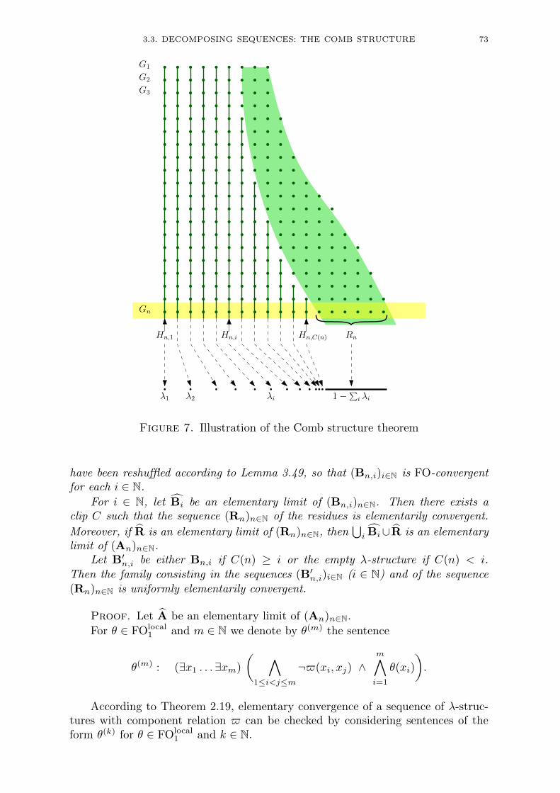
3.3. DECOMPOSING SEQUENCES: THE COMB STRUCTURE 73
G1
G2
G3
Gn
Hn,1 Hn,i Hn,C(n) Rn
λ1 λ2 λi 1−∑i λi
Figure 7. Illustration of the Comb structure theorem
have been reshuffled according to Lemma 3.49, so that (Bn,i)i∈N is FO-convergentfor each i ∈ N.
For i ∈ N, let Bi be an elementary limit of (Bn,i)n∈N. Then there exists aclip C such that the sequence (Rn)n∈N of the residues is elementarily convergent.
Moreover, if R is an elementary limit of (Rn)n∈N, then⋃i Bi∪R is an elementary
limit of (An)n∈N.Let B′n,i be either Bn,i if C(n) ≥ i or the empty λ-structure if C(n) < i.
Then the family consisting in the sequences (B′n,i)i∈N (i ∈ N) and of the sequence(Rn)n∈N is uniformly elementarily convergent.
Proof. Let A be an elementary limit of (An)n∈N.
For θ ∈ FOlocal1 and m ∈ N we denote by θ(m) the sentence
θ(m) : (∃x1 . . . ∃xm)
( ∧
1≤i<j≤m¬$(xi, xj) ∧
m∧
i=1
θ(xi)
).
According to Theorem 2.19, elementary convergence of a sequence of λ-struc-tures with component relation $ can be checked by considering sentences of theform θ(k) for θ ∈ FOlocal
1 and k ∈ N.

74 3. MODELINGS FOR SPARSE STRUCTURES
Note that for every k < k′ and every λ-structure A, if it holds A |= θ(k′) thenit holds A |= θ(k). Define
M(θ) = supk ∈ N, A |= θ(k)Ω(θ) = i ∈ N, Bi |= (∃x)θ(x).
Note that obviously |Ω(θ)| ≤M(θ).For r ∈ N, let θ1, . . . , θF (r) be an enumeration of the local first-order formulas
with a single free variable with quantifier rank at most r (up to logical equivalence).Define
A(r) = max(r, maxa≤F (r)
max Ω(θa)).
Let
C0(n) = sup
K, (∀n′ ≥ n)
K∑
i=1
∣∣∣∣|Bn′,i||An′ |
− spi
∣∣∣∣ ≤∑
i>K
spi
be the standard (maximal) clip on (An)n∈N (see Proposition 3.2).Let B(r) be the minimum integer such that
(1) it holds C0(B(r)) ≥ A(r) (note that limn→∞ C0(n) = ∞, according toProposition 3.2);
(2) for every n ≥ B(r), a ≤ F (r) and every k ≤ r it holds An |= θ(k)a if and
only if M(θa) ≥ k (note that this holds for sufficiently large n as A is anelementary limit of (An)n∈N);
(3) for every i ≤ A(r) and a ≤ F (r) it holds
Bn,i |= (∃x)θa(x) ⇐⇒ Bi |= (∃x)θa(x).
(note that this holds for sufficiently large n as Bi is an elementary limitof (Bn,i)n∈N and as we consider only finitely many values of i);
we define the non-decreasing function C : N→ N by
C(n) = maxA(r) : B(r) ≤ n.As limr→∞A(r) = ∞ and as C0(B(r)) ≥ A(r) it holds limr→∞B(r) = ∞. More-over, for every r ∈ N it holds C0(B(r)) ≥ A(r) hence C0(n) ≥ C(n). According toProposition 3.2, it follows that the function C is a clip on (An)n∈N.
Let (Rn)n∈N be the resiude of (An)n∈N with respect to the clip C, and let B′n,ibe defined as Bn,i if i ≤ C(n) and the empty λ-structure otherwise. Then it isimmediate from the definition of the clip C that the family (B′n,i)n∈N : i ∈ Nis uniformly elementarily convergent. Using Lemma 3.18, it is also easily checkedthat the residue (Rn)n∈N of (An)n∈N with respect to the clip C is elementarilyconvergent and thus, that the family (B′n,i)n∈N : i ∈ N∪(Rn)n∈N is uniformlyelementarily convergent.
The extension of the Comb structure theorem to FO-convergence now followsdirectly.
Theorem 3.58 (Comb structure for λ-structure sequences with infinite spec-trum). Let (An)n∈N be an FO-convergent sequence of finite λ-structures with com-ponent relation $ and infinite spectrum (spi)i∈N.

3.3. DECOMPOSING SEQUENCES: THE COMB STRUCTURE 75
Then there exists a clip C : N → N with residue Rn and, for each n ∈ N, apermutation fn : [C(n)] → [C(n)] such that, extending fn to N by putting f(i) tobe the identity for i > C(n), and letting B′n,i be either Bn,fn(i) if C(n) ≥ i or theempty λ-structure if C(n) < i, it holds:
• An = Rn ∪⋃i∈N B′n,i;
• limn→∞maxi>C(n) |B′n,i|/|An| = 0;• limn→∞ |Rn|/|An| exists;• for every i ∈ N, (B′n,i)n∈N is FO-convergent;• either limn→∞ |Rn|/|An| = 0 and (Rn)n∈N is elementarily convergent, or
the sequence (Rn)n∈N is FO-convergent;• the family (B′n,i)n∈N : i ∈ N ∪ (Rn)n∈N is uniformly elementarily
convergent.
This ends the (admittedly very technical and complicated) analysis of the com-ponent structure of limits. This was not developped for its own sake, but it will beall needed in the Part 3 of this paper, to construct modeling FO-limits for conver-gent sequences of trees with bounded height and for convergent sequences of graphswith bounded tree-depth.


CHAPTER 4
Limits of Graphs with Bounded Tree-depth
In this part, we mainly consider the signature λ, which consists in a binaryrelation ∼ (symmetric adjacency relation), a unary relation R (property of beinga root), and c unary relations Ci (the coloring). Colored rooted trees with heightat most h are particular λ-structures, and the class of (finite or infinite) coloredrooted trees with height at most h will be denoted by Y(h). (Here we shall be onlyconcerned with trees that are either finite, countable, or of size continuum.)
4.1. FO1-limits of Colored Rooted Trees with Bounded Height
In this section, we explictly define modeling FO1-limits for FO1-convergentsequences of colored rooted trees with bounded height and characterize modelingswhich are FO1-limits for FO1-convergent sequences of (finite) colored rooted treeswith bounded height.
4.1.1. Preliminary Observations. We take some time for some preliminaryobservations on the logic structure of rooted colored trees with bounded height.These observations will use arguments based on Ehrenfeucht-Fraısse games andstrategy stealing. (For definitions of ≡n and Ehrenfeucht-Fraısse games, see Sec-tion 2.3.1.)
For a rooted colored tree Y ∈ Y(h) and a vertex x ∈ Y , we denote Y(x) thesubtree of Y rooted at x, and by Y \ Y(x) the rooted tree obtained from Y byremoving all the vertices in Y(s).
The following two lemmas show that, like for isomorphism, equivalence betweentwo colored rooted trees can be reduced to equivalence of branches.
Lemma 4.1. Let Y,Y′ ∈ Y(h), let s, s′ be sons of the roots of Y and Y′,respectively.
Let n ∈ N. If Y(s) ≡n Y′(s′) and Y \Y(s) ≡n Y′ \Y′(s′), then Y ≡n Y′.
Proof. Assume Y(s) ≡n Y′(s′) and Y \ Y(s) ≡n Y′ \ Y′(s′). In order toprove Y ≡n Y′ we play an n-steps Ehrenfeucht-Fraısse-game EF0 on Y and Y′
as Duplicator. Our strategy will be based on two auxiliary n-steps Ehrenfeucht-Fraısse-games, EF1 and EF2, on Y(s) and Y′(s′) and on Y \Y(s) and Y′ \Y′(s′),respectively, against Duplicators following a winning strategy. Each time Spoilerselects a vertex in game EF0, we play the same vertex in the game EF1 or EF2
(depending on the tree the vertex belongs to), then we mimic the selection ofthe Duplicator of this game. it is easily checked that this strategy is a winningstrategy.
Lemma 4.2. Let Y,Y′ ∈ Y(h), let s, s′ be sons of the roots of Y and Y′,respectively.
Let n ∈ N. If Y ≡n+h Y′ and Y(s) ≡n Y′(s′), then Y \Y(s) ≡n Y′ \Y′(s′)
77
78 4. LIMITS OF GRAPHS WITH BOUNDED TREE-DEPTH
Proof. Assume Y ≡n+h Y′ and Y(s) ≡n Y′(s′).We first play (as Spoiler) s in Y then s′ in Y′. Let t′ and t be the corresponding
plays of Duplicator. Then the further n steps of the game have to map vertices inY(s), Y(t), Y\(Y(s)∪Y(t)) to Y′(t′), Y′(s′), Y′\(Y′(t′)∪Y′(s′)) (and converse),for otherwise h− 2 steps would allow Spoiler to win the game. Also, by restrictingour play to one of these pairs of trees, we deduce Y(s) ≡n Y′(t′), Y(t) ≡n Y′(s′),and Y \ (Y(s) ∪Y(t)) ≡n Y \ (Y′(s′) ∪Y′(t′)). As Y′(s′) ≡n Y(s) it follows
Y(t) ≡n Y′(s′) ≡n Y(s) ≡n Y′(t′).
Hence, according to Lemma 4.1, as Y \ (Y(s) ∪ Y(t)) = (Y \ Y(s)) \ Y(t) andY′\(Y′(s′)∪Y′(t′)) = (Y′\Y′(s′))\Y′(t′), we deduce Y\Y(s) ≡n Y′\Y′(s′).
Let λ• denote the signature obtained from λ by adding a new unary relation S(marking a special vertex, which is not necessarily the root). Let θ• be the sentence
(∃x)(S(x) ∧ (∀y S(y)→ (y = x)),
which states that a λ• contains a unique special vertex. We denote by Y(h)• the
class obtained by marking as special a single vertex of a colored rooted tree withheight at most h. Let Unmark be the interpretation of λ-structures in λ•-structures
consisting in forgetting S (so that Umark projects Y(h)• onto Y(h)).
Lemma 4.3. Let Y,Y′ ∈ Y(h)• be such that Y (resp. Y′) has special vertex
m (resp. m′). Assume that both m and m′ have height t > 1 (in Y and Y′,respectively). Let v (resp. v′) be son of the root of Y (resp. Y′) that is an ancestorof m (resp. m′).
Then for every n ∈ N, if Unmark(Y) ≡n+h Unmark(Y′) and Y(v) ≡n Y′(v′),then Y ≡n Y′.
Proof. Assume Unmark(Y) ≡n+h Unmark(Y′) and Y(v) ≡n Y′(v′). Thenit holds Unmark(Y(v)) ≡n Unmark(Y′(v′)) thus, according to Lemma 4.2,
Y \Y(v) = Unmark(Y) \Unmark(Y(v))
≡n Unmark(Y′) \Unmark(Y′(v′)) = Y′ \Y′(v′).
Hence, according to Lemma 4.1, it holds Y ≡n Y′ (as the marking could be con-sidered as a coloring).
The next lemma states that the properties of a colored rooted trees with adistinguished vertex v (which is not necessarily the root) can be retrieved from theproperties of the subtree rooted at v, the subtree rooted at the father of v, etc. (seeFig. 1).
Lemma 4.4. Let Y,Y′ ∈ Y(h), vt ∈ Y and v′t ∈ Y ′ be vertices with height t.For 1 ≤ i < t, let vi (resp. v′i) be the ancestor of vt (resp. of v′t) at height i.
Then for every integer n it holds
(∀1 ≤ i ≤ t) Y(vi) ≡n+h+1−i Y′(v′i) =⇒ (Y, vt) ≡n (Y′, v′t)
(Y, vt) ≡n+(t−1)h (Y′, v′t) =⇒ (∀1 ≤ i ≤ t) Y(vi) ≡n+(t−i)h Y′(v′i)
Proof. We proceed by induction over t. If t = 1, then the statement obviouslyholds. So, assume t > 1 and that the statement holds for t− 1.
Let Y•,Y′• ∈ Y(h)• be the marked rooted colored trees obtained from Y and
Y′ by marking vt (resp. v′t) as a special vertex.
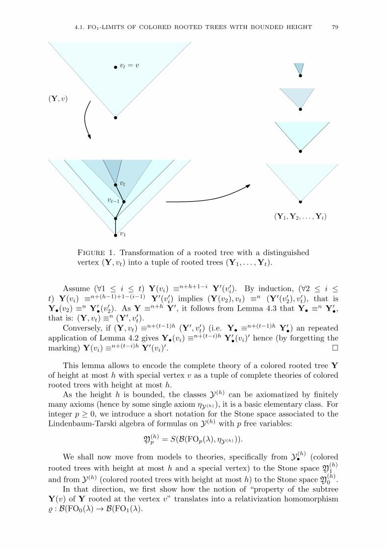
4.1. FO1-LIMITS OF COLORED ROOTED TREES WITH BOUNDED HEIGHT 79
v1
vt
vt−1
vt = v
(Y, v)
(Y1,Y2, . . . ,Yt)
Figure 1. Transformation of a rooted tree with a distinguishedvertex (Y, vt) into a tuple of rooted trees (Y1, . . . ,Yt).
Assume (∀1 ≤ i ≤ t) Y(vi) ≡n+h+1−i Y′(v′i). By induction, (∀2 ≤ i ≤t) Y(vi) ≡n+(h−1)+1−(i−1) Y′(v′i) implies (Y(v2), vt) ≡n (Y′(v′2), v′t), that isY•(v2) ≡n Y′•(v
′2). As Y ≡n+h Y′, it follows from Lemma 4.3 that Y• ≡n Y′•,
that is: (Y, vt) ≡n (Y′, v′t).Conversely, if (Y, vt) ≡n+(t−1)h (Y′, v′t) (i.e. Y• ≡n+(t−1)h Y′•) an repeated
application of Lemma 4.2 gives Y•(vi) ≡n+(t−i)h Y′•(vi)′ hence (by forgetting the
marking) Y(vi) ≡n+(t−i)h Y′(vi)′.
This lemma allows to encode the complete theory of a colored rooted tree Yof height at most h with special vertex v as a tuple of complete theories of coloredrooted trees with height at most h.
As the height h is bounded, the classes Y(h) can be axiomatized by finitelymany axioms (hence by some single axiom ηY(h)), it is a basic elementary class. Forinteger p ≥ 0, we introduce a short notation for the Stone space associated to theLindenbaum-Tarski algebra of formulas on Y(h) with p free variables:
Y(h)p = S(B(FOp(λ), ηY(h))).
We shall now move from models to theories, specifically from Y(h)• (colored
rooted trees with height at most h and a special vertex) to the Stone space Y(h)1
and from Y(h) (colored rooted trees with height at most h) to the Stone space Y(h)0 .
In that direction, we first show how the notion of “property of the subtreeY(v) of Y rooted at the vertex v” translates into a relativization homomorphism% : B(FO0(λ)→ B(FO1(λ).

80 4. LIMITS OF GRAPHS WITH BOUNDED TREE-DEPTH
We consider the simple interpretation I• of λ-structures in λ•-structures, whichmaps a λ•-structure Y• to the λ-structure defined as follows: let x ' y be definedas (x ∼ y) ∨ (x = y). Then
• the domain of I•(Y•) is defined by the formula
S(x1) ∨ (∀y1, . . . , yh)((R(y1) ∧
h−1∧
i=1
¬S(yi) ∧ (yi ' yi+1))→ (yh 6= x1)
);
• the adjacency relation ∼ is defined as in Y• (i.e. by the formula (x1 ∼x2));
• the relation R of I•(Y•) is defined by the formula S(x1).
Although I• maps general λ•-structures to λ-structures, we shall be only concerned
by the specific property that I• maps a rooted tree Y• ∈ Y(h)• with special vertex v
to the rooted tree Unmark(Y•)(v).In a sake for simplicity, for Y ∈ Y(h) we denote by (Y, v) (where Y is a λ-
structure) the λ•-structure obtained by adding the new relation S with v being theunique special vertex.
Lemma 4.5. There is a Boolean algebra homomorphism
% : B(FO0(λ), ηY(h))→ B(FO1(λ), ηY(h))
(called relativization), such that for every sentence φ ∈ FO0(λ), every Y ∈ Y(h),and every v ∈ Y it holds
Y(u) |= φ ⇐⇒ Y |= %(φ)(u).
Proof. The lemma follows from the property
Y(u) |= φ ⇐⇒ I•(Y, u) |= φ ⇐⇒ (Y, u) |= I•(φ).
The formula ρ(φ) is obtained from the sentence I•(φ) by replacing each occurenceof S(y) by y = x1.
Using relativization and Lemma 4.4, we can translate the transformation shown
on Figure 1 to a encoding of elements of Y(h)1 into tuples of elements Y
(h)0 . Intu-
itively, a element T ∈ Y(h)1 defines the properties of a colored rooted tree Y with
special vertex x1, and the relativization ρ allows us to extract from T the tupleof the complete theories of the subtrees of Y rooted at x1, the father of x1, etc.Moreover, the meaning of Lemma 4.4 is that what we obtain only depends on thecomplete theory of (Y, x1), that is only on T .
Definition 4.6. For 1 ≤ i ≤ h, let ηi ∈ FO1(λ) be the formula stating thatthe height of x1 is i.
We define the mapping Encode : Y(h)1 → ⊎h
k=1(Y(h)0 )k as follows:
For T ∈ Y(h)1 , let k be the (unique) integer such that ηk ∈ T . Then Encode(T )
is the k-tuple (T0, . . . , Tk−1), where
• Tk−1 is the set of sentences θ ∈ FO0(λ) such that ρ(θ) ∈ T (intuitively,the complete theory of the subtree rooted at x1);
• Tk−2 is the set of sentences θ ∈ FO0(λ) such that((∃y1)(ηk−1(y1) ∧ y1 ∼ x1 ∧ ρ(θ)(y)
)∈ T
(intuitively, the complete theory of the subtree rooted at father of x1);
4.1. FO1-LIMITS OF COLORED ROOTED TREES WITH BOUNDED HEIGHT 81
• Tk−1−i is the set of sentences θ ∈ FO0(λ) such that
((∃y1 . . . yi)(
i∧
j=1
ηk−j(yj) ∧i−1∧
j=1
(yj ∼ yj+1 ∧ y1 ∼ x1 ∧ ρ(θ)(yi))∈ T
(intuitively, the complete theory of the subtree rooted at the ancestor ofx1 which has height k − i);
• T0 = T∩ ∈ FO0(λ) (intuitively, the complete theory of the whole rootedtree).
Lemma 4.7. Encode is a homeomorphism of Y(h)1 and Encode(Y
(h)1 ), which is
a closed subspace of⊎hk=1(Y
(h)0 )k.
Proof. This lemma is a direct consequence of Lemma 4.4.
4.1.2. The Universal Relational Sample Space Yh. The aim of this sec-tion is to construct a rooted colored forest on a standard Borel space Yh that isFO1-universal, in the sense that every FO1-convergent sequence of colored rootedtrees will have a modeling FO1-limit obtained by assigning an adapted probabilitymeasure to one of the connected components of Yh.
Definition 4.8. For theories T, T ′ ∈ Y(h)0 , we define w(T, T ′) ≥ k if and only if
there exists a model Y of T , such that the root of Y has k (distinct) sons v1, . . . , vkwith Th(Y(vi)) = T ′.
Lemma 4.9. For k ∈ N and φ ∈ FO0, let ζk(φ) be the sentence (∃≥ky) ρ(φ)(y).Then w(T, T ′) ≥ k if and only if ζk(φ) ∈ T holds for every φ ∈ T ′.
Proof. If w(T, T ′) ≥ k, then ζk(φ) ∈ T holds for every φ ∈ T ′, hence we onlyhave to prove the opposite direction. Assume that ζk(φ) ∈ T holds for every φ ∈ T ′,but that there is φ0 ∈ T ′ such that ζk+1(φ0) /∈ T . Let Y be a model of T , andlet v1, . . . , vk be the sons of the root of Y such that Y (vi) |= φ0. For every r ∈ N,r ≥ qrank(φ0), let ψr be the conjunction of the sentences in T ′ with quantifier rankr. Obviously, ψr ∈ T ′. Moreover, as ζk(ψr) ∈ T , it holds Y |= ζk(ψr). As ψr ` φ0,it follows that for every 1 ≤ i ≤ k it holds Y (vi) |= ψr (only possible choices).As this holds for every r, we infer that for every 1 ≤ i ≤ k, Y (vi) is a model ofT ′ hence w(T, T ′) ≥ k. Now assume that for every k ∈ N and every φ ∈ T ′ it
holds ζk(φ) ∈ T . Let Y be a model of T , let Y ′ be a model of T ′, and let Y be
obtained from Y by adding (at the root of Y ) a son u with subtree Y (u) isomorphic
to Y ′. By an easy application of an Ehrenfeucht-Fraısse game, we get that Y iselementarily equivalent to Y , hence a model of T . Thus w(T, T ′) ≥ k.
Let N be the one point compactification of N, that is N = N ∪ ∞ with opensets generated by complements of finite sets.
Lemma 4.10. The function w : Y(h)0 ×Y
(h)0 → N is upper semicontinuous (with
respect to product topology of Stone space Y(h)0 ).
Proof. For r ∈ N define the function wr : Y(h)0 ×Y
(h)0 → N by:
wr(T, T′) = supk ∈ N : ∀ψ ∈ T ′ (qrank(ψ) ≤ r)⇒ ζk(ψ) ∈ T.
It follows from Lemma 4.9 that it holds
w(T, T ′) = infr∈N
wr(T, T′).
82 4. LIMITS OF GRAPHS WITH BOUNDED TREE-DEPTH
Hence, in order to prove that the function w is upper semicontinuous, it is sufficient
to prove that functions wr are continuous. Let (T0, T′0) ∈ Y
(h)0 ×Y
(h)0 .
– Assume wr(T0, T′0) = k.
If dist(T ′, T ′0) < 2−r and dist(T, T0) < 2−maxqrank(ζk+1(ψ): qrank(ψ)≤r, then it holdswr(T, T
′) = wr(T0, T′0);
– Assume wr(T0, T′0) =∞, and let k ∈ N.
If dist(T ′, T ′0) < 2−r and dist(T, T0) < 2−maxqrank(ζk+1(ψ): qrank(ψ)≤r, then it holdswr(T, T
′) > k.
For z = (z1, . . . , za) ∈ Na define the subset Fz of (Y(h)0 )a+1 by
Fz = (T0, . . . , Ta) : w(Ti−1, Ti) = zi.For t ∈ N, define
Xt =
1, . . . , t, if t ∈ N,
[0, 1], if t =∞.
For z = (z1, . . . , za) ∈ Na, define Xz =∏ai=1Xzi . Let
Vh = Y(h)0 ]
h−1⊎
a=1
⊎
z∈Na(Fz ×Xz).
Definition 4.11. The universal forest Yh has vertex set Vh. The roots of Yhare the elements in Y
(h)0 . The edges of Yh are the pairs of the form
((T0, T1, . . . , Ta), (α1, . . . , αa)), ((T0, T1, . . . , Ta+1), (α1, . . . , αa+1))
where Ti ∈ Y(h)0 , αi ∈ [0, 1] and a ∈ 0, . . . , h− 1.
Moreover, the vertex set Vh inherits the topological structure of⊎hi=1(Y
(h)0 )i×
[0, 1]i−1, which defines a σ-algebra Σh on Vh (as the trace on Vh of the Borel σ-
algebra of⊎hi=1(Y
(h)0 )i × [0, 1]i−1).
Remark 4.12. Let T0 be the complete complete theory of a colored rootedtree with height at most h. Then, by construction, T0 is the complete theory ofthe connected component of Yh rooted at T0. In particular, no two connectedcomponents of Yh are elementarily equivalent.
The remaining of this section will be devoted to the proof of Theorem 4.14,which states that Yh is a relational sample space. In order to prove this result, weshall need a preliminary lemma, which expresses that the property of a tuple ofvertices in a colored rooted tree with bounded height is completely determined bythe individual properties of the vertices in the tuple and the heights of the lowestcommon ancestors of every pair of vertices in the tuples.
Lemma 4.13. Fix rooted trees Y,Y′ ∈ Y(h). Let u1, . . . , up be p vertices of Y,let u′1, . . . , u
′p be p vertices of Y′, and let n ∈ N.
Assume that for every 1 ≤ i ≤ p it holds (Y, ui) ≡n+h (Y′, u′i) and that forevery 1 ≤ i, j ≤ p the height of ui ∧ uj in Y is the same as the height of u′i ∧ u′j inY′ (where u ∧ v denotes the lowest common ancestor of u and v).
Then (Y, ui, . . . , up) ≡n (Y′, u′1, . . . , u′p).
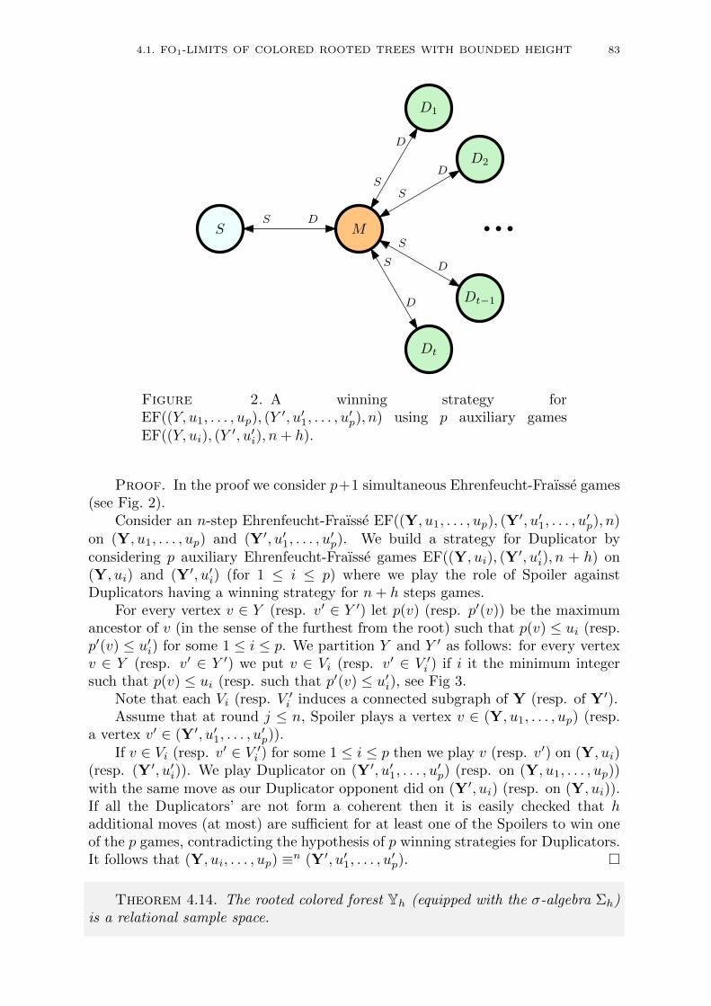
4.1. FO1-LIMITS OF COLORED ROOTED TREES WITH BOUNDED HEIGHT 83
S M
D1
D2
Dt−1
Dt
S
DS
D
S
DS
D
S D
Figure 2. A winning strategy forEF((Y, u1, . . . , up), (Y
′, u′1, . . . , u′p), n) using p auxiliary games
EF((Y, ui), (Y′, u′i), n+ h).
Proof. In the proof we consider p+1 simultaneous Ehrenfeucht-Fraısse games(see Fig. 2).
Consider an n-step Ehrenfeucht-Fraısse EF((Y, u1, . . . , up), (Y′, u′1, . . . , u
′p), n)
on (Y, u1, . . . , up) and (Y′, u′1, . . . , u′p). We build a strategy for Duplicator by
considering p auxiliary Ehrenfeucht-Fraısse games EF((Y, ui), (Y′, u′i), n + h) on
(Y, ui) and (Y′, u′i) (for 1 ≤ i ≤ p) where we play the role of Spoiler againstDuplicators having a winning strategy for n+ h steps games.
For every vertex v ∈ Y (resp. v′ ∈ Y ′) let p(v) (resp. p′(v)) be the maximumancestor of v (in the sense of the furthest from the root) such that p(v) ≤ ui (resp.p′(v) ≤ u′i) for some 1 ≤ i ≤ p. We partition Y and Y ′ as follows: for every vertexv ∈ Y (resp. v′ ∈ Y ′) we put v ∈ Vi (resp. v′ ∈ V ′i ) if i it the minimum integersuch that p(v) ≤ ui (resp. such that p′(v) ≤ u′i), see Fig 3.
Note that each Vi (resp. V ′i induces a connected subgraph of Y (resp. of Y′).Assume that at round j ≤ n, Spoiler plays a vertex v ∈ (Y, u1, . . . , up) (resp.
a vertex v′ ∈ (Y′, u′1, . . . , u′p)).
If v ∈ Vi (resp. v′ ∈ V ′i ) for some 1 ≤ i ≤ p then we play v (resp. v′) on (Y, ui)(resp. (Y′, u′i)). We play Duplicator on (Y′, u′1, . . . , u
′p) (resp. on (Y, u1, . . . , up))
with the same move as our Duplicator opponent did on (Y′, ui) (resp. on (Y, ui)).If all the Duplicators’ are not form a coherent then it is easily checked that hadditional moves (at most) are sufficient for at least one of the Spoilers to win oneof the p games, contradicting the hypothesis of p winning strategies for Duplicators.It follows that (Y, ui, . . . , up) ≡n (Y′, u′1, . . . , u
′p).
Theorem 4.14. The rooted colored forest Yh (equipped with the σ-algebra Σh)is a relational sample space.
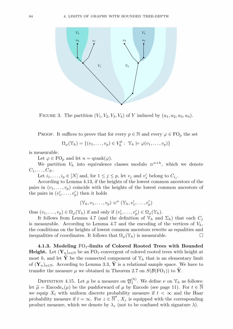
84 4. LIMITS OF GRAPHS WITH BOUNDED TREE-DEPTH
u1u2 u3 u4
V1
V2
V3
V4
Figure 3. The partition (V1, V2, V3, V4) of Y induced by (u1, u2, u3, u4).
Proof. It suffices to prove that for every p ∈ N and every ϕ ∈ FOp the set
Ωϕ(Yh) = (v1, . . . , vp) ∈ V ph : Yh |= ϕ(v1, . . . , vp)is measurable.
Let ϕ ∈ FOp and let n = qrank(ϕ).We partition Vh into equivalence classes modulo ≡n+h, which we denote
C1, . . . , CN .Let i1, . . . , ip ∈ [N ] and, for 1 ≤ j ≤ p, let vj and v′j belong to Cij .According to Lemma 4.13, if the heights of the lowest common ancestors of the
pairs in (v1, . . . , vp) coincide with the heights of the lowest common ancestors ofthe pairs in (v′1, . . . , v
′p) then it holds
(Yh, v1, . . . , vp) ≡n (Yh, v′1, . . . , v′p)
thus (v1, . . . , vp) ∈ Ωϕ(Yh) if and only if (v′1, . . . , v′p) ∈ Ωϕ(Yh).
It follows from Lemma 4.7 (and the definition of Vh and Σh) that each Cjis measurable. According to Lemma 4.7 and the encoding of the vertices of Vh,the conditions on the heights of lowest common ancestors rewrite as equalities andinequalities of coordinates. It follows that Ωϕ(Yh) is measurable.
4.1.3. Modeling FO1-limits of Colored Rooted Trees with BoundedHeight. Let (Yn)n∈N be an FO1-convergent of colored rooted trees with height at
most h, and let Y be the connected component of Yh that is an elementary limit
of (Yn)n∈N. According to Lemma 3.3, Y is a relational sample space. We have to
transfer the measure µ we obtained in Theorem 2.7 on S(B(FO1)) to Y.
Definition 4.15. Let µ be a measure on Y(h)1 . We define ν on Yh as follows:
let µ = Encode∗(µ) be the pushforward of µ by Encode (see page 11). For t ∈ Nwe equip Xt with uniform discrete probability measure if t < ∞ and the Haarprobability measure if t = ∞. For z ∈ Na, Xz is equipped with the correspondingproduct measure, which we denote by λz (not to be confused with signature λ).

4.1. FO1-LIMITS OF COLORED ROOTED TREES WITH BOUNDED HEIGHT 85
We define the measure ν as follows: let A be a measurable subset of Vh, let
A0 = A ∩Y(h)0 , and let Az = A ∩ (Fz ×Xz). Then
ν(A) = µ(A0) +h−1∑
a=1
∑
z∈Na(µ⊗ λz)(Az).
(Notice that the sets Az are measurable as Fz ×Xz is measurable for every z.)
Lemma 4.16. The measure µ is the push-forward of ν by the projection P :
Yh → Y(h)1 defined by
P ((T0, T1, α1, . . . , Ta, αa)) = Encode−1(T0, . . . , Ta),
that is: µ = P∗(ν).
Proof. First notice that P is continuous, as Encode is a homeomorphism
(by Lemma 4.7). Let B be a measurable set of Y(h)1 . Let A = P−1(B). Then
A ∩ (Fz ×Xz) = (Encode(B) ∩ Fz)×Xz hence
(µ⊗ λz)(A ∩ (Fz ×Xz)) = ν(Encode(B) ∩ Fz)λz(Xz) = µ(Encode(B) ∩ Fz).It follows that
P∗(ν)(B) = ν(A)
= µ(A ∩Y(h)0 ) +
h−1∑
a=1
∑
z∈Na(µ⊗ λz)(A ∩ (Fz ×Xz))
= µ(Encode(B) ∩Y(h)0 ) +
h−1∑
a=1
∑
z∈Naµ(Encode(B) ∩ Fz)
= µ(Encode(B) ∩ (Y
(h)0 ]
h−1⊎
a=1
⊎
z∈NaFz))
= µ Encode(B)
= µ(B).
(as z ranges over a countable set and as all the Fz are measurable). Hence µ =P∗(ν).
Lemma 4.17. Let µ be a pure measure on Y(h)1 and let T0 the complete theory
of µ (see Definition 2.9). Let ν be the measure defined from µ by Definition 4.15.
Let Y be the connected component of Yh containing the support of ν. Let νY be the
restriction of ν to Y.
Then Y, equipped with the probability measure νY is a modeling such that forevery ϕ ∈ FO1 it holds
〈ϕ, Y〉 = µ(K(ϕ)).
Let X ⊂ Y(h)1 be the set of all T ∈ Y
(h)1 such that x1 is not the root (i.e. X =
T ∈ Y(h)1 : R(x1) /∈ T). Let f : X → Y
(h)0 be the second projection of Encode (if
Encode(T ) = (T0, . . . , Ti) then f(T ) = T1). Let κ = f∗(µ) be the pushforward of
µ by f . Intuitively, for T ∈ Y(h)0 , κ(T) is the global measure of all the subtrees
with complete theory T that are rooted at a son of the root.
86 4. LIMITS OF GRAPHS WITH BOUNDED TREE-DEPTH
Let rY be the root of Y. Then it holds
supv∼r
Y
νY(Y(v)) = supT∈X
κ(T)w(T0, T )
.
Proof. As µ is pure, the complete theory of µ is the theory T0 to whichevery point of the support of µ projects. Hence the support of µ defines a unique
connected component Y of Yh. That for every ϕ ∈ FO1 it holds
〈ϕ, Y〉 = µ(K(ϕ))
is a direct consequence of Lemma 4.16.The second equation is a direct consequence of the construction of νY.
Theorem 4.18. Let Yn be an FO1-convergent sequence of colored rooted trees
with height at most h, and let µ be the limit measure of µYnon Y
(h)1 . Let ν be the
measure defined from µ by Definition 4.15. Let Y be the connected component of
Yh containing the support of ν. Let νY be the restriction of ν to Y.
Then Y, equipped with the probability measure νY, is a modeling FO1-limit of(Yn)n∈N.
Moreover, it holds
supv∼r
Y
νY(Y(v)) ≤ lim infn→∞
maxv∼rYn
|Yn(v)||Yn|
.
Proof. As (Yn)n∈N is elementarily convergent, the complete theory of theelementary limit of this sequence is the theory T0 to which every point of the
support of µ projects, hence µ is pure. According to Lemma 4.17, Y is an FO1-modeling limit of (Yn)n∈N.
Let κ be defined as in Lemma 4.17. If κ is atomless, then supv∼rYνY(Y(v)) = 0
hence the inequation holds.Let T be such that κ(T) > 0. For every ε > 0 there exists θε ∈ T such that
κ(T) ≤ κ(T ′ : T ′ 3 θε) ≤ κ(T) + ε.
Moreover, it follows from Lemma 4.9 that
w(T0, T ) = limε→0
∑w(T0, T
′) : T ′ 3 θε.
Then, as (Yn)n∈N is elementarily convergent to a rooted tree with theory T0 itholds
w(T0, T ) = limε→0
limn→∞
|v ∈ Yn : v ∼ rYnand Yn(v) |= θε|
= limε→0
limn→∞
|v ∈ Yn : Yn |= (v ∼ rYn) ∧ ρ(θε)(v)|.
As limn→∞ |v ∈ Yn : Yn |= (v ∼ rYn) ∧ ρ(θε)(v)| is non-increasing when ε→ 0,
and is a non-negative integer or ∞, there exists ε0 such that for every 0 < ε < ε0 itholds
w(T0, T ) = limn→∞
|v ∈ Yn : Yn |= (v ∼ rYn) ∧ ρ(θε)(v)|.

4.1. FO1-LIMITS OF COLORED ROOTED TREES WITH BOUNDED HEIGHT 87
For ε > 0, let φε be the formula stating that the subtree rooted at a son of theroot that contains x1 satisfies θε. Then it holds
κ(T ′ : T ′ 3 θε) = µ(K(φε))
= limn→∞
〈φε,Yn〉
= limn→∞
∑|Yn(v)| : Yn |= (v ∼ rYn) ∧ ρ(θε)(v)
|Yn|
Hence, for every 0 < ε < ε0 it holds
κ(T)w(T0, T )
≤ limn→∞
ε+∑ |Yn(v)|
|Yn| : Yn |= (v ∼ rYn) ∧ ρ(θε)(v)
|v ∈ Yn : Yn |= (v ∼ rYn) ∧ ρ(θε)(v)|
≤ ε+ lim infn→∞
max
|Yn(v)||Yn|
: Yn |= (v ∼ rYn) ∧ ρ(θε)(v)
≤ ε+ lim infn→∞
maxv∼rYn
|Yn(v)||Yn|
.
Hence
κ(T)w(T0, T )
≤ lim infn→∞
maxv∼rYn
|Yn(v)||Yn|
.
4.1.4. Inverse Theorems for FO1-limits of Colored Rooted Trees withBounded Height. We characterize here the measures µ on S(B(FO1)), which areweak limits of measures µYn for some FO1-convergent sequence (Yn)n∈N of coloredrooted trees with height at most h.
Fact 4.19. If (Yn)n∈N is an FO1-convergent sequence of colored rooted treeswith height at most h, then µ is pure and its complete theory is the limit inS(B(FO0)) of the complete theories of the rooted trees Yn.
We need the following combinatorial condition for a probability measure on aStone space.
Definition 4.20. A probability measure µ on S(B(FOp(λ))) (p ≥ 1) orS(B(FO(λ))) satisfies the Finitary Mass Transport Principle (FMTP) if for everyφ, ψ ∈ FO1(λ) and every integers a, b such that
φ ` (∃≥ay) (x1 ∼ y) ∧ ψ(y)
ψ ` (∃≤by) (x1 ∼ y) ∧ ψ(y)
it holdsaµ(K(φ)) ≤ b µ(K(ψ)).
Similarly, a modeling L satisfies the FMTP if, for every φ, ψ, a, b as above itholds (see Fig. 4):
a〈φ,L〉 ≤ b〈ψ,L〉.
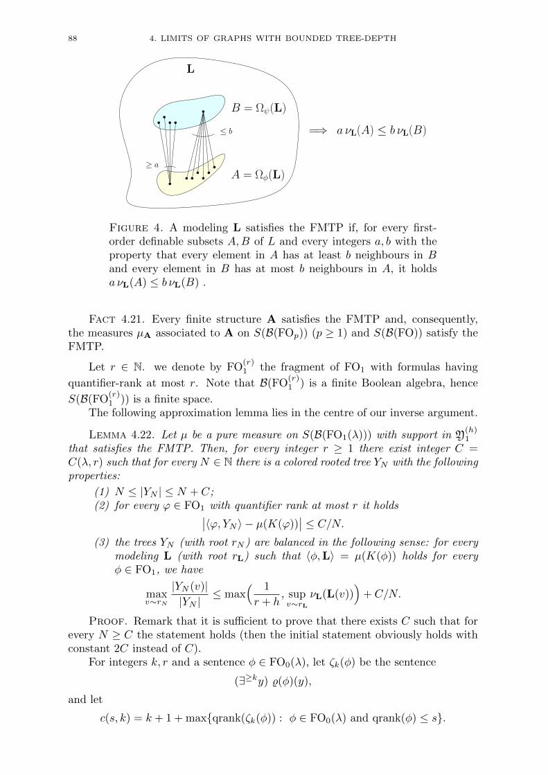
88 4. LIMITS OF GRAPHS WITH BOUNDED TREE-DEPTH
L
B = Ωψ(L)
A = Ωφ(L)≥ a
≤ b =⇒ a νL(A) ≤ b νL(B)
Figure 4. A modeling L satisfies the FMTP if, for every first-order definable subsets A,B of L and every integers a, b with theproperty that every element in A has at least b neighbours in Band every element in B has at most b neighbours in A, it holdsa νL(A) ≤ b νL(B) .
Fact 4.21. Every finite structure A satisfies the FMTP and, consequently,the measures µA associated to A on S(B(FOp)) (p ≥ 1) and S(B(FO)) satisfy theFMTP.
Let r ∈ N. we denote by FO(r)1 the fragment of FO1 with formulas having
quantifier-rank at most r. Note that B(FO(r)1 ) is a finite Boolean algebra, hence
S(B(FO(r)1 )) is a finite space.
The following approximation lemma lies in the centre of our inverse argument.
Lemma 4.22. Let µ be a pure measure on S(B(FO1(λ))) with support in Y(h)1
that satisfies the FMTP. Then, for every integer r ≥ 1 there exist integer C =C(λ, r) such that for every N ∈ N there is a colored rooted tree YN with the followingproperties:
(1) N ≤ |YN | ≤ N + C;(2) for every ϕ ∈ FO1 with quantifier rank at most r it holds∣∣〈ϕ, YN 〉 − µ(K(ϕ))
∣∣ ≤ C/N.(3) the trees YN (with root rN ) are balanced in the following sense: for every
modeling L (with root rL) such that 〈φ,L〉 = µ(K(φ)) holds for everyφ ∈ FO1, we have
maxv∼rN
|YN (v)||YN |
≤ max( 1
r + h, supv∼rL
νL(L(v)))
+ C/N.
Proof. Remark that it is sufficient to prove that there exists C such that forevery N ≥ C the statement holds (then the initial statement obviously holds withconstant 2C instead of C).
For integers k, r and a sentence φ ∈ FO0(λ), let ζk(φ) be the sentence
(∃≥ky) %(φ)(y),
and let
c(s, k) = k + 1 + maxqrank(ζk(φ)) : φ ∈ FO0(λ) and qrank(φ) ≤ s.
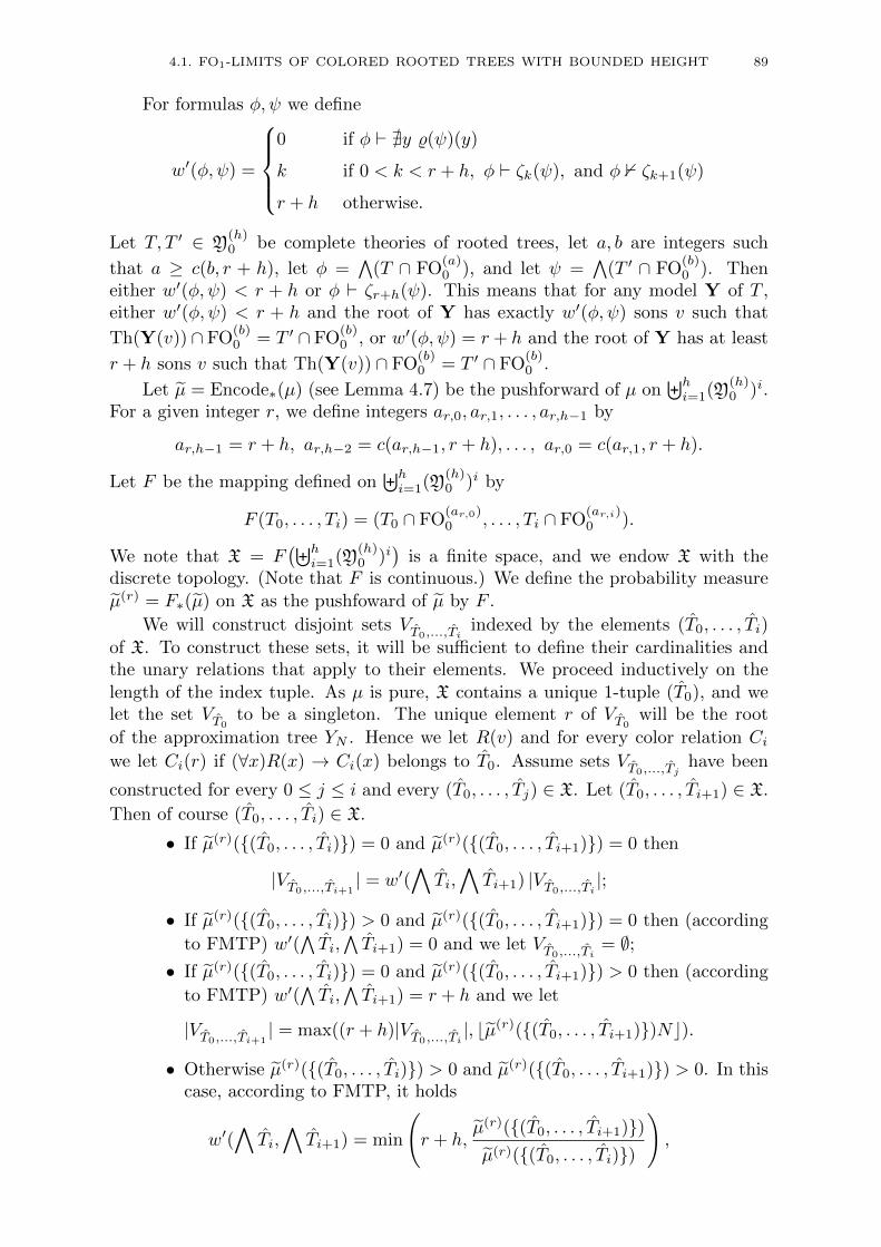
4.1. FO1-LIMITS OF COLORED ROOTED TREES WITH BOUNDED HEIGHT 89
For formulas φ, ψ we define
w′(φ, ψ) =
0 if φ ` @y %(ψ)(y)
k if 0 < k < r + h, φ ` ζk(ψ), and φ 0 ζk+1(ψ)
r + h otherwise.
Let T, T ′ ∈ Y(h)0 be complete theories of rooted trees, let a, b are integers such
that a ≥ c(b, r + h), let φ =∧
(T ∩ FO(a)0 ), and let ψ =
∧(T ′ ∩ FO
(b)0 ). Then
either w′(φ, ψ) < r + h or φ ` ζr+h(ψ). This means that for any model Y of T ,either w′(φ, ψ) < r + h and the root of Y has exactly w′(φ, ψ) sons v such that
Th(Y(v)) ∩ FO(b)0 = T ′ ∩ FO
(b)0 , or w′(φ, ψ) = r + h and the root of Y has at least
r + h sons v such that Th(Y(v)) ∩ FO(b)0 = T ′ ∩ FO
(b)0 .
Let µ = Encode∗(µ) (see Lemma 4.7) be the pushforward of µ on⊎hi=1(Y
(h)0 )i.
For a given integer r, we define integers ar,0, ar,1, . . . , ar,h−1 by
ar,h−1 = r + h, ar,h−2 = c(ar,h−1, r + h), . . . , ar,0 = c(ar,1, r + h).
Let F be the mapping defined on⊎hi=1(Y
(h)0 )i by
F (T0, . . . , Ti) = (T0 ∩ FO(ar,0)0 , . . . , Ti ∩ FO
(ar,i)0 ).
We note that X = F(⊎h
i=1(Y(h)0 )i
)is a finite space, and we endow X with the
discrete topology. (Note that F is continuous.) We define the probability measureµ(r) = F∗(µ) on X as the pushfoward of µ by F .
We will construct disjoint sets VT0,...,Tiindexed by the elements (T0, . . . , Ti)
of X. To construct these sets, it will be sufficient to define their cardinalities andthe unary relations that apply to their elements. We proceed inductively on thelength of the index tuple. As µ is pure, X contains a unique 1-tuple (T0), and welet the set VT0
to be a singleton. The unique element r of VT0will be the root
of the approximation tree YN . Hence we let R(v) and for every color relation Ciwe let Ci(r) if (∀x)R(x) → Ci(x) belongs to T0. Assume sets VT0,...,Tj
have been
constructed for every 0 ≤ j ≤ i and every (T0, . . . , Tj) ∈ X. Let (T0, . . . , Ti+1) ∈ X.
Then of course (T0, . . . , Ti) ∈ X.
• If µ(r)((T0, . . . , Ti)) = 0 and µ(r)((T0, . . . , Ti+1)) = 0 then
|VT0,...,Ti+1| = w′(
∧Ti,∧Ti+1) |VT0,...,Ti
|;
• If µ(r)((T0, . . . , Ti)) > 0 and µ(r)((T0, . . . , Ti+1)) = 0 then (according
to FMTP) w′(∧Ti,∧Ti+1) = 0 and we let VT0,...,Ti
= ∅;• If µ(r)((T0, . . . , Ti)) = 0 and µ(r)((T0, . . . , Ti+1)) > 0 then (according
to FMTP) w′(∧Ti,∧Ti+1) = r + h and we let
|VT0,...,Ti+1| = max((r + h)|VT0,...,Ti
|, bµ(r)((T0, . . . , Ti+1))Nc).
• Otherwise µ(r)((T0, . . . , Ti)) > 0 and µ(r)((T0, . . . , Ti+1)) > 0. In thiscase, according to FMTP, it holds
w′(∧Ti,∧Ti+1) = min
(r + h,
µ(r)((T0, . . . , Ti+1))µ(r)((T0, . . . , Ti))
),

90 4. LIMITS OF GRAPHS WITH BOUNDED TREE-DEPTH
Then, if w′(∧Ti,∧Ti+1) < r + h we let
|VT0,...,Ti+1| = w′(
∧Ti,∧Ti+1)|VT0,...,Ti
|
and otherwise we let
|VT0,...,Ti+1| = max((r + h)|VT0,...,Ti
|, bµ(r)((T0, . . . , Ti+1))Nc).
The colors of the elements of VT1,...,Tiare easily defined: for v ∈ VT1,...,Ti
and color
relation Ci we let Ci(v) if (∀x)R(x)→ Ci(x) belongs to Ti.The tree YN has vertex set
⋃VT1,...,Ti
. Each set VT0,...,Ti+1is partitionned as
equaly as possible into |VT0,...,Ti| parts, each part being adjacent to a single vertex in
VT0,...,Ti. It follows that the degree in VT0,...,Ti+1
of a vertex in VT0,...,Tilies between
d|VT0,...,Ti+1|/|VT0,...,Ti
|e and b|VT0,...,Ti+1|/|VT0,...,Ti
|c, and that (by construction and
thanks to FMTP) this coincides with w′(∧Ti,∧Ti+1) (when < r+h) or is at least
w′(∧Ti,∧Ti+1) (when = r + h).
For (T0, . . . , Ti) ∈ X, it is easily checked that∣∣|VT0,...,Ti
| − µ((T0, . . . , Ti))N∣∣ ≤ (r + h)i.
For φ ∈ FO1(λ), let Fφ = F Encode(T ) : T ∈ K(φ) ∩ Y(h)1 . Let C =
(r + h)h|X|. Then, by summing up the above inequality, we get
0 ≤( ∑
(T0,...,Ti)∈Fϕ
|VT0,...,Ti|)− µ(K(ϕ))N ≤ C.
In particular, if φ is the true statement, we get
N ≤ |YN | ≤ N + C.
Also, we deduce that for every T0, T1) ∈ X and every v1, v2 ∈ VT0,T1it holds
∣∣|YN (v1)| − |YN (v2)|∣∣ ≤ C.
Let Z = T ∈ Y(h)1 : T ∩FO0(λ) = T0, let T ∈ Z, let (T0, . . . , Ti) = Encode(T ),
and let (T0, . . . , Ti) = F (T0, . . . , Ti). We now prove that if v ∈ VT0,...,Tiand
(T ′0, . . . , T′i ) = Encode(Th(YN , v)) then it holds Tj ∩ FO
(r+h)0 = T ′j ∩ FO
(r+h)0 for
every 1 ≤ j ≤ i (see Fig 4.1.4).
First note that it is sufficient to prove Ti∩FO(r+h)0 = T ′i ∩FO
(r+h)0 , as the other
equalities follow by considering the ancestors of v. If Ti (hence T ′i ) is the completetheory of a single vertex tree, then by construction of VT0,...,Ti
, it holds Ti = T ′i .Assume now that i is such that for every (T0, . . . , Ti+1) ∈ Encode(T ) with T ∈ Z,
it holds Ti+1 ∩ FO(r+h)0 = T ′i+1 ∩ FO
(r+h)0 . Let A be a model of Ti and let B be a
model of T ′i . It follows from the induction that the roots of A and B have the samenumber of sons (up to r+ h) with subtrees, which are (r+ h)-equivalent to a fixedrooted tree. By an easy argument based on an Ehrefeucht-Fraısse game, it follows
that A and B are (r + h)-equivalent hence Ti ∩ FO(r+h)0 = T ′i ∩ FO
(r+h)0 .
According to Lemma 4.4, we deduce that for T ∈ Z and corresponding vertex
v ∈ VT0,...,Tiit holds Th(YN , v) ∩ FO
(r)1 = T ∩ FO
(r)1 .
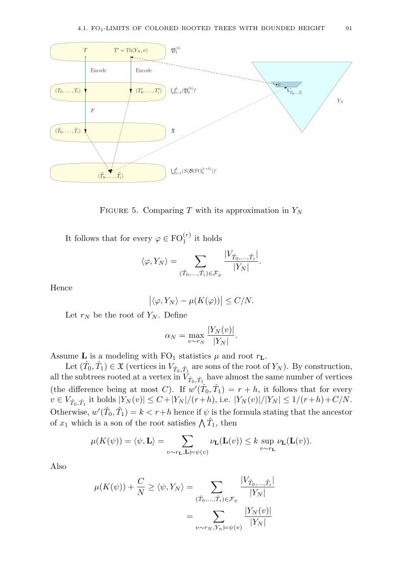
4.1. FO1-LIMITS OF COLORED ROOTED TREES WITH BOUNDED HEIGHT 91
Y(h)1T T ′ = Th(YN , v)
⋃hi=1(Y
(h)0 )i(T ′
0, . . . , T′i )
Encode
(T0, . . . , Ti) X
YN
VT0,...,Ti
v(T0, . . . , Ti)
Encode
F
⋃hi=1(S(B(FO
(r+h)0 ))i
(T0, . . . , Ti)
Figure 5. Comparing T with its approximation in YN
It follows that for every ϕ ∈ FO(r)1 it holds
〈ϕ, YN 〉 =∑
(T0,...,Ti)∈Fϕ
|VT0,...,Ti|
|YN |.
Hence ∣∣〈ϕ, YN 〉 − µ(K(ϕ))∣∣ ≤ C/N.
Let rN be the root of YN . Define
αN = maxv∼rN
|YN (v)||YN |
.
Assume L is a modeling with FO1 statistics µ and root rL.Let (T0, T1) ∈ X (vertices in VT0,T1
are sons of the root of YN ). By construction,all the subtrees rooted at a vertex in VT0,T1
have almost the same number of vertices
(the difference being at most C). If w′(T0, T1) = r + h, it follows that for everyv ∈ VT0,T1
it holds |YN (v)| ≤ C+ |YN |/(r+h), i.e. |YN (v)|/|YN | ≤ 1/(r+h)+C/N .
Otherwise, w′(T0, T1) = k < r+h hence if ψ is the formula stating that the ancestor
of x1 which is a son of the root satisfies∧T1, then
µ(K(ψ)) = 〈ψ,L〉 =∑
v∼rL,L|=ψ(v)
νL(L(v)) ≤ k supv∼rL
νL(L(v)).
Also
µ(K(ψ)) +C
N≥ 〈ψ, YN 〉 =
∑
(T0,...,Ti)∈Fψ
|VT0,...,Ti|
|YN |
=∑
v∼rN ,Yn|=ψ(v)
|YN (v)||YN |

92 4. LIMITS OF GRAPHS WITH BOUNDED TREE-DEPTH
hence µ(K(ψ)) + CN ≥ maxv∼rN ,Yn|=ψ(v)
|YN (v)||YN | if k = 1, and otherwise
µ(K(ψ)) +C
N≥ k max
v∼rN ,Yn|=ψ(v)
|YN (v)| − C|YN |
≥ k maxv∼rN ,Yn|=ψ(v)
|YN (v)||YN |
− C/N.
Hence, considering the case k = 1 and the case k ≥ 2 (where 2C/k ≤ C) we get
maxv∼rN ,Yn|=ψ(v)
|YN (v)||YN |
≤ supv∼rL
νL(L(v)) + C/N.
And we deduce
αN ≤ max( 1
r + h, supv∼rL
νL(L(v)))
+ C/N.
We get the following two inverse results:
Theorem 4.23. A measure µ on S(B(FO1)) is the weak limit of a sequence ofmeasures µYn associated to an FO1-convergent sequence (Yn)n∈N of finite coloredrooted trees with height at most h (i.e. of finite Yn ∈ Y(h)) if and only if
• µ is pure and its complete theory belongs to Y(h)0 ,
• µ satisfies the FMTP.
Proof. Assume that (Yn)n∈N is an FO1-convergent sequence of finite Yn ∈Y(h), and that µYN ⇒ µ. According to Remark 2.10, µ is pure. As (Yn)n∈N iselementarily convergent, the complete theory of µ is the complete theory of theelementary limit of (Yn)n∈N. Also, µ satisfies the FMTP (see Section 2.1.4).
Conversely, assume µ is pure, that its complete theory belongs to Y(h)0 , and
that it satisfies the FMTP. According to Lemma 4.22 we can construct a sequence(Yn)n∈N of finite Yn ∈ Y(h) (considering for instance r = n and N = 10C where Cis the constant defined from r, h, c) such that for every formula φ ∈ FO1(λ) it holds∣∣〈φ, Yn〉 − µ(K(φ))
∣∣→ 0 as n→∞, i.e. µYn ⇒ µ.
and we deduce
Theorem 4.24. A modeling L is the FO1-limit of an FO1-convergent sequence(Yn)n∈N of finite colored rooted trees with height at most h (i.e. of finite Yn ∈ Y(h))if and only if
• L is a colored rooted tree with height at most h (i.e. L ∈ Y(h)),• L satisfies the FMTP.
Proof. That an FO1-convergent sequence of finite rooted colored trees Yn ∈Y(h) has a modeling FO1-limit is a direct consequence of Theorem 4.18. That Lsatisfies the FMTP is immediate (as the associate measure µ = Tp1
L ∗(νL) does).Conversely, that a colored rooted tree modeling L ∈ Y(h) that satisfies the
FMTP is the FO1-limit of a sequence of finite rooted colored trees Yn ∈ Y(h) is adirect consequence of Theorem 4.23.

4.2. FO-LIMITS OF COLORED ROOTED TREES WITH BOUNDED HEIGHT 93
4.2. FO-limits of Colored Rooted Trees with Bounded Height
In this section we explicitly define modeling FO-limits for FO-convergent se-quences of colored rooted trees with bounded height.
We first sketch our method.We consider the signature λ+, which is the signature λ augmented by a new
unary relation P . Particular λ+-structures are colored rooted forests with a princi-pal connected component, whose root will be marked by relation P instead of R (noother vertex gets P ). The class of colored rooted forests with a principal connectedcomponent and height at most h will be denoted by F (h).
We consider three basic interpretation schemes:
(1) IY→F is a basic interpretation scheme of λ+-structures in λ-structuresdefined as follows: for every λ-structure A, the domain of IY→F (A) is thesame as the domain of A, and it holds (for every x, y ∈ A):
IY→F (A) |= x ∼ y ⇐⇒ A |= (x ∼ y) ∧ ¬R(x) ∧ ¬R(y)
IY→F (A) |= R(x) ⇐⇒ A |= (∃z) R(z) ∧ (z ∼ x)
IY→F (A) |= P (x) ⇐⇒ A |= R(x)
In particular, IY→F maps a colored rooted tree Y ∈ Y(h) into a coloredrooted forest IY→F (A)(Y ) ∈ F (h−1), formed by the subtrees rooted at thesons of the former root and a single vertex rooted principal component(the former root);
(2) IF→Y is a basic interpretation scheme of λ-structures in λ+-structuresdefined as follows: for every λ+-structure A, the domain of IF→Y (A) isthe same as the domain of A, and it holds (for every x, y ∈ A):
IF→A(A) |= x ∼ y ⇐⇒ A |= (x ∼ y) ∨R(x) ∧ P (y) ∨R(y) ∧ P (x)
IF→A(A) |= R(x) ⇐⇒ A |= P (x)
In particular, IF→Y maps a colored rooted forest F ∈ F (h) into a coloredrooted tree IF→Y (F ) ∈ Y(h+1) by making each non principal root a sonof the principal root;
(3) IR→P is a basic interpretation scheme of λ+-structures in λ-structuresdefined as follows: for every λ+-structure A, the domain of IR→P (A) isthe same as the domain of A, adjacencies are the same in A and IR→P (A),no element of IR→P (A) is in R, and for every x ∈ A it holds
IR→P (A) |= P (x) ⇐⇒ A |= R(x).
(Roughly speaking, the relation R becomes the relation P .) In particular,IR→P maps a colored rooted tree Y ∈ Y(h) into a colored rooted forestIR→P (Y ) ∈ F (h) having a single (principal) component.
We now outline our proof strategy. Let (Yn)n∈N be an FO-convergent sequenceof finite rooted colored trees (Yn ∈ Y(h)) such that limn→∞ |Yn| =∞.
For each n, IY→F (Yn) is a forest Fn, and (Yn)n∈N is an FO-convergent se-quence. According to the Comb Structure Theorem, there exists a countable set(Yn,i)n∈N of FO-convergent sequences of colored rooted trees Yn,i ∈ Y(h) and a
FO-convergent sequence (Rn)n∈N of residues Rn ∈ F (h), which are special coloredrooted forests (as the isolated principal root obviously belongs to Rn), so that

94 4. LIMITS OF GRAPHS WITH BOUNDED TREE-DEPTH
• the sequences (Yn,i)n∈N and the sequence (Rn)n∈N form a uniformly con-vergent family of sequences;
• for each n ∈ N it holds IY→F (Yn) = Rn ∪⋃i∈I Yn,i.
If the limit spectrum of (IY→F (Yn))n∈N is empty (i.e. I = ∅), the sequence(Yn)n∈N of colored rooted trees is called residual, and in this case we deduce directlythat a residual sequence of colored rooted trees admit a modeling FO-limit fromour results on FO1-convergent sequences.
Otherwise, we proceed by induction over the height bound h. Denote by(spi)i∈I the limit spectrum of (IY→F (Yn))n∈N, let sp0 = 1 −∑i∈I spi, and letYn,0 = IR→P IF→Y (Rn). As (IF→Y (Rn))n∈N is residual, (Yn,0)n∈N has a mod-
eling FO-limit Y0. By induction, each (Yn,i)n∈N has a modeling FO-limit Yi. AsYn = IF→Y (
⋃i∈I∪0Yn,i), we deduce (using uniform elementary convergence)
that (Yn)n∈N has modeling FO-limit IF→Y (∐i∈I∪0(Yi, spi)).
This finishes the outline of our construction. Now we provide details.
4.2.1. The Modeling FO-limit of Residual Sequences. We start by aformal definition of residual sequences of colored rooted trees.
Definition 4.25. Let (Yn)n∈N be a sequence of finite colored rooted trees, letNn be the set of all sons of the root of Yn, and let Yn(v) denote (for v ∈ Yn) thesubtree of Yn rooted at v.
The sequence (Yn)n∈N is residual if
lim supn→∞
maxv∈Nn
|Yn(v)||Yn|
= 0.
We extend this definition to single infinite modelings.
Definition 4.26. A modeling colored rooted tree Y with height at most h isresidual if, denoting by N the neighbour set of the root, it holds
supv∈N
νY(Y(v)) = 0.
Note that the above definition makes sense as belonging to a same Y(v) (for
some v ∈ N) is first-order definable hence, as Y is a relational sample space, each
Y(v) is ΣY-measurable.We first prove that for a modeling colored rooted tree to be a modeling FO-
limit of a residual sequence (Yn)n∈N of rooted colored trees with bounded height,it is sufficient that it is a modeling FO1-limit of the sequence.
Lemma 4.27. Assume (Yn)n∈N is a residual FO1-convergent sequence of finite
rooted colored trees with bounded height with residual modeling FO1-limit Y.
Then (Yn)n∈N is FO-convergent and has modeling FO-limit Y.
Proof. Let h be a bound on the height of the rooted trees Yn. Let Fn =IY→F (Yn). Let $ be the formula asserting dist(x1, x2) ≤ 2h. Then Fn |= $(u, v)holds if and only if u and v belong to a same connected component of Fn. Accordingto Lemma 3.47, we get that (Fn)n∈N is FOlocal convergent. As it is also FO0-convergent, it is FO convergent (according to Theorem 2.21). As Yn = IF→Y (Fn),we deduce that (Yn)n∈N is FO-convergent.
That Y is a modeling FO-limit of (Yn)n∈N then follows from Theorem 3.17.

4.2. FO-LIMITS OF COLORED ROOTED TREES WITH BOUNDED HEIGHT 95
Lemma 4.28. Let Yn be a residual FO1-convergent sequence of colored rooted
trees with height at most h, let µ be the limit measure of µYnon T
(h)1 , and let Y
be the connected component of Yh containing the support of ν. Then Y, equippedwith the probability measure νY = ν, is a modeling FO-limit of (Yn)n∈N.
Proof. That Y is a residual FO1-modeling limit of (Yn)n∈N is a consequenceof Theorem 4.18. That it is then an FO-modeling limit of (Yn)n∈N follows fromLemma 4.27
4.2.2. The Modeling FO-Limit of a Sequence of Rooted Trees. For anintuition of how the structure of a modeling FO-limit of a sequence of colored rootedtrees with height at most h could look like, consider a modeling rooted colored treeY. Obviously, the Y contains two kind of vertices: the heavy vertices v such thatthe subtree Y(v) of Y rooted at v has positive νY-measure and the light verticesfor which Y(v) has zero νY-measure. It is then immediate that heavy vertices ofY induce a countable rooted subtree with same root as Y.
This suggest the following definitions.
Definition 4.29. A rooted skeleton is a countable rooted tree S together witha mass function m : S → (0, 1] such that m(r) = 1 (r is the root of S) and for everynon-leaf vertex v ∈ S it holds
m(v) ≥∑
u son of v
m(u).
Definition 4.30. Let (S,m) be a rooted skeleton, let S0 be the subset of Swith vertices v such that m(v) =
∑u son of vm(u), let (Rv)v∈S\S0
be a countablesequence of non-empty residual λ-modeling indexed by S \ S0, and let (Rv)v∈S0
be a countable sequence of non empty countable colored rooted trees indexed byS0. The grafting of (Rv)v∈S\S0
and (Rv)v∈S0on (S,m) is the modeling Y defined
as follows: As a graph, Y is obtained by taking the disjoint union of S with thecolored rooted trees Rv and then identifying v ∈ S with the root of Rv (see Fig. 6).The sigma algebra ΣY is defined as
ΣY = ⋃
v∈S\S0
Mv ∪⋃
v∈S0
M ′v : Mv ∈ ΣRv ,M′v ⊆ Rv
and the measure νY(M) of M ∈ Σ is defined by
νY(M) =∑
v∈S\S0
(m(v)−
∑
u son of v
m(u))νRv (Mv),
where M =⋃v∈S\S0
Mv ∪⋃v∈SM
′v with Mv ∈ ΣRv and M ′v ⊆ Rv.
Lemma 4.31. Let Y be obtained by grafting countable sequence of non-emptymodeling colored rooted trees Rv on a rooted skeleton (S,m). Then Y is a modeling.
Proof. We prove the statement by induction over the height of the rootedskeleton. The statement obviously holds if S is a single vertex rooted tree (that is ifheight(S) = 1). Assume that the statement holds for rooted skeletons with heightat most h, and let (S,m) be a rooted skeleton with height h+ 1.
Let s0 be the root of S and let si : i ∈ I ⊆ N be the set of the sons of s0 inS. For i ∈ I, Yi = Y(si) be the subtree of Y rooted at si, let spi =
∑x∈Yi m(x),

96 4. LIMITS OF GRAPHS WITH BOUNDED TREE-DEPTH
S Y
v
Rv
Figure 6. Grafting of trees on a skeleton
and let mi be the mass function on Si defined by mi(v) = m(v)/spi. Also, letsp0 = 1−∑i∈I spi.
For each i ∈ I ∪ 0, if spi = 0 (in which case Rsi is only assumed to bea relational sample space) we turn Rsi into a modeling by defining a probabilitymeasure on Rsi concentrated on si.
For i ∈ I, let Yi be obtained by grafting the Rv on (Si,mi) (for v ∈ Si), and letY0 be the λ+-modeling consisting in a rooted colored forest with single (principal)component Rs0 (that is: Y0 = IR→P (Rs0)). According to Lemma 3.11, Y0 is amodeling, and by induction hypothesis each Yi (i ∈ I) is a modeling. According toLemma 3.21, it follows that F = qi∈I∪0(Yi, spi) is a modeling. Hence, accordingto Lemma 3.11, Y = IF→Y (F) is a modeling.
Our main theorem is the following.
Theorem 4.32. Let (Yn)n∈N be an FO-convergent sequence of finite coloredrooted trees with height at most h.
Then there exists a skeleton (S,m) and a family (Rv)v∈S — where Rv is (iso-morphic to) a connected component of Yh, ΣRv
is the induced σ-algebra on Rv —with the property that the grafting Y of the Rv on (S,m) is a modeling FO-limitof the sequence (Yn)n∈N.
Proof. First notice that the statement obviously holds if limn→∞ |Yn| < ∞as then the sequence is eventually constant to a finite colored rooted tree Y: wecan let S be Y (without the colors), m be the uniform weight (m(v) = 1/|Y |), andRv be single vertex rooted tree whose root’s color is the color of v in Y. So, wecan assume that limn→∞ |Yn| =∞.
We prove the statement by induction over the height bound h. For h = 1, eachYn is a single vertex colored rooted tree, and the statement obviously holds.
Assume that the statements holds for h = h0 − 1 ≥ 1 and let finite coloredrooted trees with height at most h0. Let Fn = IY→F (Yn). Then (Fn)n∈N is FO-convergent (according to Lemma 3.11). According to the Comb Structure Theorem,there exists countably many convergent sequences (Yn,i)n∈N of colored rooted trees(for i ∈ I) and an FO-convergent sequence (Rn)n∈N of special rooted forests forminga uniformly convergent family of sequences, such that IY→F (Yn) = Rn∪
⋃i∈I Yn,i.
If the limit spectrum of (IY→F (Yn))n∈N is empty (i.e. I = ∅), the sequence(Yn)n∈N of colored rooted trees is residual, and the result follows from Lemma 4.28.
4.2. FO-LIMITS OF COLORED ROOTED TREES WITH BOUNDED HEIGHT 97
Otherwise, let (spi)i∈I the limit spectrum of (IY→F (Yn))n∈N, let sp0 =1 −∑i∈I spi, and let Yn,0 = IR→P IF→Y (Rn). If sp = 0 then there is a con-
nected component Y0 of Yh that is an elementary limit of (Yn,0)n∈N; Otherwise, as(IF→Y (Rn))n∈N is residual, (Yn,0)n∈N has, according to Lemma 4.28, a modeling
FO-limit Y0. By induction, each (Yn,i)n∈N has a modeling FO-limit Yi. As Yn =IF→Y (
⋃i∈I∪0Yn,i), we deduce, by Corollary 3.4, Lemma 3.27, Theorem 2.21, and
Lemma 3.11, that (Yn)n∈N has modeling FO-limit IF→Y (∐i∈I∪0(Yi, spi)).
So, in the case of colored rooted trees with bounded height, we have constructedan explicit relational sample space that allows to pullback the limit measure µdefined on the Stone space S(B(FO)).
4.2.3. Inverse theorem for FO-limits of Colored Rooted Trees withBounded Height. Recall that for λ-modelings A and B, and p, r ∈ N we defined
‖A−B‖localp,r = sup|〈φ,A〉 − 〈φ,B〉| : φ ∈ FOlocal
p (λ), qrank(φ) ≤ r.Lemma 4.33. Let L ∈ Y(h) (with root rL) be a colored rooted tree modeling
that satisfies the FMTP, let p, r ∈ N, and let ε > 0. Then there exist C0 =C0(λ, p, r, ε), N0 = N0(λ, p, r, ε) such that for every N ≥ N0 there exists there existsa finite colored rooted tree Y ∈ Y(h) such that it holds N ≤ |Y | ≤ N +C0, Y ≡r L,and
‖Y − L‖localp,r < max(ε, 2 sup
v∼rLνL(L(v))).
Proof. Without loss of generality we can assume ε ≥ 2 supv∼rL νL(L(v)). Letr′ = max(r, 4cr,p/ε), where cr,p is the constant introduced in Lemma 3.23..
According to Lemma 4.22, there is C0 = C(λ, r′) (hence C0 depends on λ, p, r,and ε) such that for every N ∈ N there exists Y ∈ Y(h) with the following properties:
(1) N ≤ |Y | ≤ N + C0;(2) for every ϕ ∈ FO1 with quantifier rank at most r′ it holds∣∣〈ϕ, Y 〉 − 〈ϕ,L〉
∣∣ ≤ C0/N.
(In particular Y ≡r′ L as N > C0.)(3) we have
maxv∼rN
|Y (v)||Y | ≤ max
( 1
r′ + h, supv∼rL
νL(L(v)))
+ C0/N.
Let N0 = 4cr,pC(λ, r′)/ε and assume N ≥ N0.Let F = IY→F (Y ) and A = IY→F (L). Let Fi, i ∈ ΓF and Ai, i ∈ ΓA be the
connected components of F and A. Then
maxi∈ΓF
|Fi||F | ≤ max
( 1
r′ + h, supi∈ΓL
νA(Ai))
+ C0/N <ε
2cr,p.
As IY→F is a quantifier-free interpretation, for every ϕ ∈ FO1 with quantifier rankat most r it holds ∣∣〈ϕ, F 〉 − 〈ϕ,A〉
∣∣ ≤ C0/N ≤ε
4cr,p.
In particular we have ‖F −A‖local1,r ≤ ε
4cr,p. According to Lemma 3.24, it holds
‖F −A‖localp,r < cr,p
(maxi∈ΓF
|Fi||F | + sup
i∈ΓL
νA(Ai) + ‖F −A‖local1,r
)< ε.

98 4. LIMITS OF GRAPHS WITH BOUNDED TREE-DEPTH
and it follows that ‖Y − L‖localp,r < ε.
Lemma 4.34. Let L ∈ Y(h) be an infinite colored rooted tree modeling thatsatisfies the FMTP, let p, r ∈ N and let ε > 0. Then there exist constants Ch, Nh(depending on λ, p, r, ε) such that for every N ≥ Nh there is a finite colored rootedtree Yε ∈ Y(h) such that N ≤ |Yε| ≤ N + Ch, Yε ≡r L, and ‖L− Yε‖local
p,r < ε.
Proof. Let α = ε2/(2(3cr,p)h), where cr,p is the constant which appears in
Lemma 3.23. A vertex v ∈ L is α-heavy if either v is the root rL of L, or the fatheru of v in L is α-heavy and νL(L(v)) > ανL(L(u)). The α-heavy vertices of L forma finite subtree S rooted at rL (each node v of S has at most 1/α sons).
We prove by induction on the height t of S that — assuming α ≤ ε/2 — thereexist constants Ct−1, Nt−1 (depending on λ, p, r, ε) such that for every N ≥ Nt−1
there is a finite colored rooted tree Yε ∈ Y(h) such that N ≤ |Yε| ≤ N + Ct−1,Yε ≡r L, and ‖L− Yε‖local
p,r < ε.If t = 1 (i.e. rL is the only α-heavy vertex) then
supv∼rL
νL(L(v)) < α.
Hence, according to Lemma 4.33, there exists N0, C0 (depending on λ, r, p, and ε)such that for every N ≥ N0 there is a finite colored rooted tree Y ∈ Y(h) such thatN ≤ |Y | ≤ N + C0, Y ≡r L, and
‖Y − L‖localp,r < max(ε, 2 sup
v∼rLνL(L(v))) = ε.
Now assume that the statement we want to prove by induction holds whenS has height at most t ≥ 1, and let L be such that the associated subtree S ofα-heavy vertices has height t + 1. Let v1, . . . , vk (where k is at most 1/α) be theα-heavy sons of the root rL of L, let Li be the relational sample space defined byLi = L(vi) for 1 ≤ i ≤ k, and let L0 be the colored rooted tree relational samplespace obtained by removing all the subtrees Li from L. Each Li is measurable inL. Let ai = νL(Li), and let
ε′ =ε
3cr,p
Ct(λ, p, r, ε) = max
(Ct−1(λ, p, r, ε′)
α,C0(λ, p, r, ε′/3cr,p)
)
Nt(λ, p, r, ε) = max
(Nt−1(λ, p, r, ε′)
ε′,Ct−1(λ, p, r, ε′)
αε′, N0(λ, p, r, ε′/3cr,p)
).
(Nothe that we do not change α.)
Assume a0 ≥ ε′. Let Li be the modeling with relational sample space Li andprobability measure νLi
which is a−1i νL|Li, where νL|Li stands for the restriction of
νL to Li. Let Si be the rooted subtree of α-heavy vertices of Li. Clearly, if 1 ≤ i ≤ k,then Si = S(vi) (as we did not change α) thus Si has height at most t. Let F ∈ F (h)
be the forest defined from F =∐ki=0(Li, ai) by making the component L0 special.
It is clear that L = IF→Y (F). For every N ≥ Nt(λ, p, r, ε) ≥ Nt−1(λ, p, r, ε′)/ε′
there exist, by induction, Y1, . . . , Yk such that aiN ≤ Yi ≤ aiN + Ct−1(λ, p, r, ε′),Yi ≡r Li, and ‖Yi − Li‖local
p,r < ε′. As the induction step is carried on at most h

4.2. FO-LIMITS OF COLORED ROOTED TREES WITH BOUNDED HEIGHT 99
times, it will always hold that α ≤ ε′2/2 hence
supv∼rL0
νL0(L0(v))) ≤ 1
ε′supv∼rL0
νL(L0(v))) ≤ α
ε′≤ ε′/2.
Also, according to Lemma 4.33, for every N ≥ Nt−1(λ, p, r, ε′) ≥ N0(λ, p, r, ε′) thereis a finite colored rooted tree Y0 ∈ Y(h) such that N ≤ |Y0| ≤ N + C0(λ, p, r, ε′) ≤N + Ct−1(λ, p, r, ε′), Y ′ ≡r L0, and
‖Y0 − L0‖localp,r < max(ε′, 2 sup
v∼rL0
νL0(L0(v))) = ε′.
Then
aiN + Ct−1(λ, p, r, ε′)/α
≤ |Yi|∑ki=0 |Yi|
≤ ai + Ct−1(λ, p, r, ε′)N
.
Thus ∣∣∣∣ai −|Yi|∑ki=0 |Yi|
∣∣∣∣ <Ct−1(λ, p, r, ε′)
αN≤ ε′.
Let G be the disjoint union of the Yi. Hence it holds, according to Lemma 3.23
‖F−G‖localp,r ≤ 2cr,pε
′ < ε.
Moreover, N ≤ |G| ≤ N + Ct−1(λ, p, r, ε′)/α ≤ N + Ct(λ, p, r, ε).If a0 < ε′ we consider Y1, . . . , Yk as above, but Y0 is chosen with the only
conditions that |Y0| ≤ C0(λ, p, r, ε′) ≤ Ct−1(λ, p, r, ε′) and Y0 ≡r L0. (Actually, Y0
can be chosen so that |Y0| is bounded by a function of λ, p, and r only.) Let G be
the disjoint union of the Yi. Let L0 be the modeling with relational sample spaceL0 and probablity measure νL0
= a−10 νL|L0 if a0 > 0, and any probability measure
if a0 = 0 (for instance the discrete probability measure concentrated on rL0). Let
F ∈ F (h) be the forest defined from F =∐ki=0(Li, ai) by making the component
L0 special. It is clear that L = IF→Y (F). Then, according to Lemma 3.23
‖F−G‖localp,r ≤ cr,p
(ε′ +
k∑
i=1
ai‖Li − Yi‖localp,r + a0
)
< cr,p(2ε′ + sup
1≤i≤k‖Li − Yi‖local
p,r
)
≤ 3cr,pε′ = ε.
and, as above, N ≤ |G| ≤ N + Ct(λ, p, r, ε). Now, let Yε = IF→Y (G). As IF→Yis basic and quantifier-free, and as IF→(Y) = L it holds ‖L − Yε‖local
p,r < ε andN ≤ |Y | ≤ N + Ct(λ, p, r, ε).
Theorem 4.35. A modeling L is the FO-limit of an FO-convergent sequence(Yn)n∈N of finite colored rooted trees with height at most h if and only if
• L is a colored rooted tree with height at most h,• L satisfies the FMTP.

100 4. LIMITS OF GRAPHS WITH BOUNDED TREE-DEPTH
4.3. Limit of Graphs with Bounded Tree-depth
Let Y be a rooted forest. The vertex x is an ancestor of y in Y if x belongsto the path linking y and the root of the tree of Y to which y belongs to. Theclosure Clos(Y) of a rooted forest Y is the graph with vertex set V (Y ) and edgeset x, y : x is an ancestor of y in Y, x 6= y. The height of a rooted forest isthe maximum number of vertices in a path having a root as an extremity. Thetree-depth td(G) of a graph G is the minimum height of a rooted forest Y suchthat G ⊆ Clos(Y). This notion is defined in [59] and studied in detail in [71]. Inparticular, graphs with bounded tree-depth serve as building blocks for low tree-depth decompositions, see [60, 61, 62]. It is easily checked that for each integer t theproperty td(G) ≤ t is first-order definable. It follows that for each integer t thereexists a first-order formula ξ with a single free variable such that for every graphG and every vertex v ∈ G it holds:
G |= ξ(v) ⇐⇒ td(G) ≤ t and td(G− v) < td(G).
Let t ∈ N. We define the basic interpretation scheme It, which interprets theclass of connected graphs with tree-depth at most t in the class of 2t−1-coloredrooted trees: given a 2t−1-colored rooted tree Y (where colors are coded by t − 1unary relations C1, . . . , Ct−1), the vertices u, v ∈ Y are adjacent in It(Y) if thethere is an integer i in 1, . . . , t− 1 such that Y |= Ci(v) and u is the ancestor of vat height i or Y |= Ci(u) and v is the ancestor of u at height i.
Theorem 4.36. Let (Gn)n∈N be an FO-convergent sequence of finite coloredgraphs with tree-depth at most h. Then there exists a colored rooted tree modelingL ∈ Y(h) satisfying the FMTP, such that the modeling G = Ih(L) has tree-depth atmost h and is a modeling FO-limit of the sequence (Gn)n∈N.
Conversely, if there is colored rooted tree modeling L ∈ Y(h) satisfying theFMTP and if G = Ih(L), then there is an FO-convergent sequence (Gn)n∈N offinite colored graphs with tree-depth at most h, such that G is a modeling FO-limitof (Gn)n∈N.
Proof. For each Gn, there is a colored rooted tree Yn ∈ Y(h) such that Gn =Ih(Yn). By compactness, the sequence (Yn)n∈N has a converging subsequence(Yin)n∈N, which admits a modeling FO-limit Y (according to Theorem 4.32), andit follows from Lemma 3.11 that Ih(Y) is a modeling FO-limit (with tree-depthat most h) of the sequence (Gin)n∈N, hence a modeling FO-limit of the sequence(Gn)n∈N.

CHAPTER 5
Concluding Remarks
5.1. Selected Problems
We hope that the theory developed here will encourage further researches. Herewe list a sample of related problems
The first problem concern existence of modeling FO-limits. Recall that a classC is nowhere dense [65, 66, 67, 69] if, for every integer d there is an integer N suchthat the d-subdivision of KN is not a subgraph of a graph in C. We have proven,see Theorem 3.32, that if a monotone class C is such that every FO-convergentsequence of graphs in C has a modeling FO-limit, then C is nowhere dense. It isthus natural to ask whether the converse statement holds.
Problem 5.1. Let C be a nowhere dense class of graphs. Is it true that everyFO-convergent sequence (Gn)n∈N of finite graphs in C admit a modeling FO-limit?
Aldous-Lyons conjecture [5] states that every unimodular distribution on rootedcountable graphs with bouded degree is the limit of a bounded degree graph se-quence. One of the reformulations of this conjecture is that every graphing is anFOlocal limit of a sequence of finite graphs. The importance of this conjecture ap-pears, for instance, in the fact that it would imply that all groups are sofic, whichwould prove a number of famous conjectures which are proved for sofic groups butstill open for all groups.
The next problem is a possible strengthening of the conjecture.
Problem 5.2. Is every graphing G with the finite model property an FO-limitof a sequence of finite graphs?
Although the existence of a modeling FO-limit for FO-convergent sequencesof graphs with bounded tree-depth follows easily from our study of FO-convergentsequence of rooted colored trees, the inverse theorem is more difficult. Indeed, ifwe would like to extend the inverse theorem for rooted colored trees to boundedtree-depth modelings, we naturally have to address the following question:
Problem 5.3. Is it true that there is a function f : N → N such that forevery graph modeling L with tree-depth at most t there exists a rooted coloredtree modeling Y with height at most f(t) such that L = If(t)(Y), where the Ih (forh ∈ N) are the basic intepretation schemes introduced in Section 4.3?
5.1.1. Classes with Bounded SC-depth. We can generalize our main con-struction of limits to other tree-like classes. For example, in a similar way that weobtained a modeling FO-limit for FO-convergent sequences of graphs with boundedtree-depth, it is possible to get a modeling FO-limit for FO-convergent sequencesof graphs with bounded SC-depth, where SC-depth is defined as follows [36]:
101

102 5. CONCLUDING REMARKS
Let G be a graph and let X ⊆ V (G). We denote by GX
the graph G′ withvertex set V (G) where x 6= y are adjacent in G′ if (i) either x, y ∈ E(G) and
x, y 6⊆ X, or (ii) x, y 6∈ E(G) and x, y ⊆ X. In other words, GX
is the graphobtained from G by complementing the edges on X.
Definition 5.1 (SC-depth). We define inductively the class SC(n) as follows:
• We let SC(0) = K1;• if G1, . . . , Gp ∈ SC(n) and H = G1∪ . . . ∪Gp denotes the disjoint union of
the Gi, then for every subset X of vertices of H we have HX ∈ SC(n+1).
The SC-depth of G is the minimum integer n such that G ∈ SC(n).
5.1.2. Classes with Bounded Expansion. A graph H is a shallow topolog-ical minor of a graph G at depth t if some ≤ 2t-subdivision of H is a subgraph of G.For a class C of graphs we denote by C O t the class of all shallow topological minorsat depth t of graphs in C. The class C has bounded expansion if, for each t ≥ 0, theaverage degrees of the graphs in the class C O t is bounded, that is (denoting d(G)the average degree of a graph G):
(∀t ≥ 0) supG∈C O t
d(G) <∞.
The notion of classes with bounded expansion were introduced by the authors in [57,58, 60], and their properties further studied in [61, 62, 23, 24, 63, 64, 66, 67, 71, 72]and in the monograph [68]. Particularly, classes with bounded expansion includeclasses excluding a topological minor, like classes with bounded maximum degree,planar graphs, proper minor closed classes, etc.
Classes with bounded expansion have the characteristic property that they ad-mit special decompositions — the so-called low tree-depth decompositions — relatedto tree-depth:
Theorem 5.2 ([58, 60]). Let C be a class of graph. Then C has bounded ex-pansion if and only if for every integer p ∈ N there exists N(p) ∈ N such that thevertex set of every graph G ∈ C can be partitioned into at most N(p) parts in sucha way that the subgraph of G induced by any i ≤ p parts has tree-depth at most i.
This decomposition theorem is the core of linear-time first-order model checkingalgorithm proposed by Dvorak, Kral’, and Thomas [25, 26]. In their survey onmethods for algorithmic meta-theorems [37], Grohe and Kreutzer proved that (ina class with bounded expansion) it is possible eliminate a universal quantificationby means of the additions of a bounded number of new relations while preservingthe Gaifman graph of the structure.
By an inductive argument, we deduce that for every integer p, r and every classC of λ-structure with bounded expansion, there is a signature λ+ ⊇ λ, such thatevery λ-structure A ∈ C can be lifted into a λ+-structure A+ with same Gaifmangraph, in such a way that for every first-order formula φ ∈ FOp(λ) with quantifier
rank at most r there is an existential formula φ ∈ FOp(λ+) such that for every
v1, . . . , vp ∈ A it holds
A |= φ(v1, . . . , vp) ⇐⇒ A+ |= φ(v1, . . . , vp).
Moreover, by considering a slightly stronger notion of lift if necessary, we can assume
that φ is a local formula. We deduce that there is an integer q = q(C, p, r) such

ACKNOWLEDGEMENTS 103
that checking φ(v1, . . . , vp) can be done by considering satisfaction of ψ(v1, . . . , vp)in subgraphs induced by q color classes of a bounded coloration. Using a low-treedepth decomposition (and putting the corresponding colors in the signature λ+),
we get that there exists finitely many induced substructures A+I (I ∈
([N ]q
)) with
tree-depth at most q and the property that for every first-order formula φ ∈ FOp(λ)
with quantifier rank at most r there is an existential formula φ ∈ FOp(λ+) such
that for every v1, . . . , vp ∈ A with set of colors I0 ⊆ I it holds
A |= φ(v1, . . . , vp) ⇐⇒ ∃I ∈(
[N ]
q − p
): A+
I∪I0 |= φ(v1, . . . , vp).
Moreover, the Stone pairing 〈φ,A〉 can be computed by inclusion/exclusion from
stone pairings 〈φ,A+I 〉 for I ∈
([N ]≤q).
Thus, if we consider an FO converging-sequence (An)n∈N, the tuple of limitsof the λ+-structures (An)+
I behaves as a kind of approximation of the limit of theλ-structures An. We believe that this presents a road map for considering moregeneral limits of sparse graphs.
Acknowledgements
The authors would like to thank Pierre Charbit for suggesting to use a proofby induction for Lemma 4.4 and Cameron Freer for his help in proving that theFO-limit of a sequence of random graphs cannot be a modeling.


Bibliography
[1] S. Adams, Trees and amenable equivalence relations, Ergodic Theory Dynam.Systems 10 (1990), 1–14.
[2] H. Adler and I. Adler, Interpreting nowhere dense graph classes as a classicalnotion of model theory, European J. Combin. (2013), to appear.
[3] D. Aldous, Representations for partially exchangeable arrays of random vari-ables, J. Multivar. Anal. 11 (1981), 581–598.
[4] , Exchangeability and related topics, Ecole d’ete de probabilites de Saint-Flour, XIII — 1983, Lecture Notes in Mathematics, vol. 1117, Springer, 1985,pp. 1–198.
[5] D. Aldous and R. Lyons, Processes on unimodular random networks, ElectronicJournal of Probability 12 (2007), 1454–1508.
[6] T. Austin, On exchangeable random variables and the statistics of large graphsand hypergraphs, Probability Surveys 5 (2008), 80–145.
[7] I. Benjamini, H. Finucane, and R. Tessera, On the scaling limit of finite vertextransitive graphs with large diameter, arXiv:1203.5624, 2012.
[8] I. Benjamini and O. Schramm, Recurrence of distibutional limits of finite pla-nar graphs, Electron. J. Probab. 6 (2001), no. 23, 13pp.
[9] A. Blass, G. Exoo, and F. Harary, Paley graphs satisfy all first-order adjacencyaxioms, J. Graph Theory 5 (1981), 435–439.
[10] B. Bollobas and A. Thomason, Graphs which contain all small graphs, Euro-pean J. Combin. 2 (1981), 13–15.
[11] C. Borgs, J. Chayes, L. Lovasz, V.T. Sos, and K. Vesztergombi, Countinggraph homomorphisms, Topics in Discrete Mathematics (M. Klazar, J. Kra-tochvıl, M. Loebl, J. Matousek, R. Thomas, and P. Valtr, eds.), Algorithmsand Combinatorics, vol. 26, Springer Verlag, 2006, pp. 315–371.
[12] C. Borgs, J.T. Chayes, L. Lovasz, V.T. Sos, B. Szegedy, and K. Vesztergombi,Graph limits and parameter testing, Proc. 38th Annual ACM Symp. Principlesof Dist. Comp., 2005, pp. 51–59.
[13] C. Borgs, J.T. Chayes, L. Lovasz, V.T. Sos, and K. Vesztergombi, Conver-gent sequences of dense graphs I: Subgraph frequencies, metric properties andtesting, Adv. Math. 219 (2008), no. 6, 1801–1851.
[14] C. Borgs, J.T. Chayes, L Lovasz, V.T. Sos, and K. Vesztergombi, Convergentsequences of dense graphs II: Multiway cuts and statistical physics, Annals ofMathematics 176 (2012), 151–219.
[15] P.J. Cameron and J. Nesetril, Homomorphism-homogeneous relational struc-tures, Combin. Probab. Comput. 15 (2006), 91–103.
[16] A.K. Chandra and P.M. Merlin, Optimal implementation of conjunctive queriesin relational databases, Proc. 9th ACM Symp. on Theory of Computing, 1977,pp. 77–90.
105

106 Bibliography
[17] P. Charbit, L. Hosseini, J. Nesetril, and P. Ossona de Mendez, On m-partitecographs, in preparation, 2013.
[18] G. Cherlin, Two problems on homogeneous structures, revisited, Model Theo-retic Methods in Finite Combinatorics (M. Grohe and J.A. Makowsky, eds.),vol. 558, American Mathematical Society, 2011, pp. 319–415.
[19] F. R. K. Chung, R. L. Graham, and R. M. Wilson, Quasi-random graphs,Combinatorica 9 (1989), no. 4, 345–362.
[20] P. Diaconis, S. Holmes, and S. Janson, Threshold graph limits and randomthreshold graphs, Internet Mathematics 5 (2009), no. 3, 267–318.
[21] P. Diaconis and S. Janson, Graph limits and exchangeable random graphs.,Rend. Mat. Appl., VII. Ser. 28 (2008), no. 1, 33–61 (English).
[22] R. Diestel, Graph theory, Springer Verlag, 1997.[23] Z. Dvorak, Asymptotical structure of combinatorial objects, Ph.D. thesis,
Charles University, Faculty of Mathematics and Physics, 2007.[24] , On forbidden subdivision characterizations of graph classes, European
J. Combin. 29 (2008), no. 5, 1321–1332.[25] Z. Dvorak and D. Kral’, Algorithms for classes of graphs with bounded expan-
sion, Lecture Notes in Computer Science 5911 LNCS (2010), 17–32.[26] Z. Dvorak, D. Kral’, and R. Thomas, Deciding first-order properties for sparse
graphs, 51st Annual IEEE Symposium on Foundations of Computer Science(FOCS 2010), 2010, pp. 133–142.
[27] A. Ehrenfeucht, An application of games to the completeness problem for for-malized theories, Fund. Math. 49 (1961), 129–141.
[28] G. Elek, Note on limits of finite graphs, Combinatorica 27 (2007), 503–507.[29] G. Elek and B. Szegedy, Limits of hypergraphs, removal and regularity lemmas.
A non-standard approach, arXiv:0705.2179v1 [math.CO], 2007.[30] P. Erdos and A. Renyi, The evolution of random graphs, Magyar Tud. Akad.
Mat. Kutato Int. Kozl 5 (1960), 17–61.[31] P. Erdos and A. Renyi, Asymmetric graphs, Acta Math. Acad. Sci. Hungar.
14 (1963), 295–315.[32] R. Fraısse, Sur une nouvelle classification des systemes de relations, Comptes
Rendus 230 (1950), 1022–1024.[33] , Sur quelques classifications des systemes de relations, Ph.D. thesis,
University of Paris, 1953, published in Publications Scientifiques de l’Universited’Alger, series A 1 (1954), 35182., pp. 1022–1024.
[34] D. Gaboriau, Invariant percolation and harmonic Dirichlet functions, Geomet-ric And Functional Analysis 15 (2005), 1004–1051.
[35] H. Gaifman, On local and non-local properties, Proceedings of the HerbrandSymposium, Logic Colloquium ’81, 1982.
[36] R. Ganian, P. Hlineny, J. Nesetril, J. Obdrzalek, P. Ossona de Mendez, andR. Ramadurai, When trees grow low: Shrubs and fast MSO1, MFCS 2012,Lecture Notes in Computer Science, vol. 7464, Springer-Verlag, 2012, pp. 419–430.
[37] M. Grohe and S. Kreutzer, Methods for algorithmic meta theorems, Model The-oretic Methods in Finite Combinatorics, Contemporary mathematics, 2011,pp. 181–206.
[38] W. Hanf, Model-theoretic methods in the study of elementary logic, The theoryof models (J.W. Addison et al., ed.), North-Holland, 1965, pp. 132–145.
Bibliography 107
[39] H. Hatami and S. Norine, The entropy of random-free graphons and properties,arXiv:1205.3529, May 2012.
[40] P. Hell and J. Nesetril, Graphs and homomorphisms, Oxford Lecture Series inMathematics and its Applications, vol. 28, Oxford University Press, 2004.
[41] W. Hodges, Model theory, Cambridge University Press, 1993.[42] D. Hoover, Relations on probability spaces and arrays of random variables,
Tech. report, Institute for Advanced Study, Princeton, NJ, 1979.[43] S. Janson, Graph limits and hereditary properties, arXiv:1102.3571, Mar 2013.[44] , Graphons, cut norm and distance, couplings and rearrangements, New
York Journal of Mathematics Monographs, vol. 4, European MathematicalInformation Service, 2013.
[45] O. Kallenberg, Probabilistic symmetries and invariance principles, Probabilityand Its Applications, Springer, 2005.
[46] A.S. Kechris, S. Solecki, and S. Todorcevic, Borel chromatic numbers, Ad-vances in Mathematics 141 (1999), 1–44.
[47] A.H. Lachlan and R.E. Woodrow, Countable ultrahomogeneous undirectedgraphs, Trans. AMS 262 (1980), 51–94.
[48] D. Lascar, La theorie des modeles en peu de maux, Cassini, 2009.[49] M.C. Laskowski, Vapnik-chervonenkis classes of definable sets, J. London
Math. Soc 45 (1992), 377–384.[50] P. Loeb, Conversion from nonstandard to standard measure spaces and appli-
cations in probability theory, Trans. AMS 211 (1975), 113–122.[51] J. Los, Quelques remarques, theoremes et problemes sur les classes definissables
d’algebres, Mathematical interpretation of formal systems, Studies in logic andthe foundations of mathematics, North-Holland, 1955.
[52] L Lovasz, Very large graphs, arXiv:0902.0132, Feb. 2009.[53] , Large networks and graph limits, Colloquium Publications, vol. 60,
American Mathematical Society, 2012.[54] L. Lovasz and B. Szegedy, Limits of dense graph sequences, J. Combin. Theory
Ser. B 96 (2006), 933–957.[55] L Lovasz and B. Szegedy, Regularity partitions and the topology of graphons,
An irregular mind (Szemeredi is 70) (I. Barany and J. Solymosi, eds.), BolyaiSociety Mathematical Studies, vol. 21, Springer, 2010, pp. 415–446.
[56] R. Lyons, Asymptotic enumeration of spanning trees, Combinatorics, Proba-bility and Computing 14 (2005), 491–522.
[57] J. Nesetril and P. Ossona de Mendez, The grad of a graph and classes withbounded expansion, 7th International Colloquium on Graph Theory (A. Ras-paud and O. Delmas, eds.), Electronic Notes in Discrete Mathematics, vol. 22,Elsevier, 2005, pp. 101–106.
[58] , Linear time low tree-width partitions and algorithmic consequences,STOC’06. Proceedings of the 38th Annual ACM Symposium on Theory ofComputing, ACM Press, 2006, pp. 391–400.
[59] , Tree depth, subgraph coloring and homomorphism bounds, EuropeanJournal of Combinatorics 27 (2006), no. 6, 1022–1041.
[60] , Grad and classes with bounded expansion I. decompositions, EuropeanJournal of Combinatorics 29 (2008), no. 3, 760–776.
[61] , Grad and classes with bounded expansion II. algorithmic aspects, Eu-ropean Journal of Combinatorics 29 (2008), no. 3, 777–791.
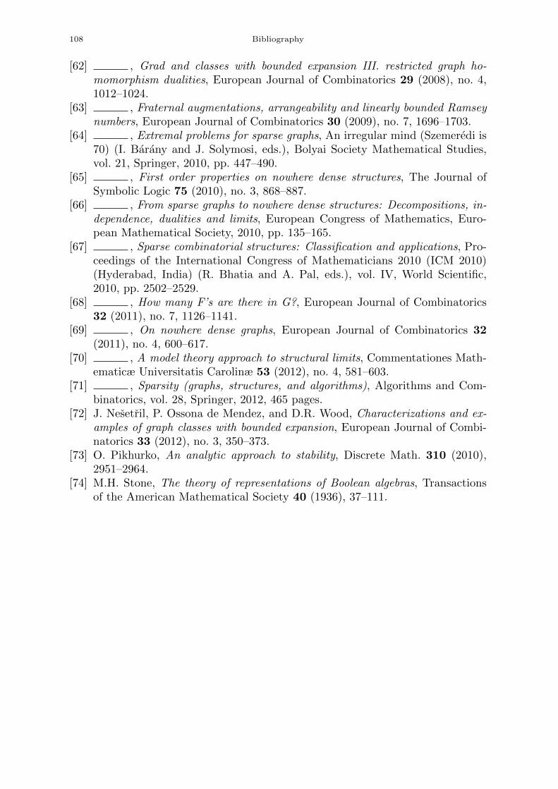
108 Bibliography
[62] , Grad and classes with bounded expansion III. restricted graph ho-momorphism dualities, European Journal of Combinatorics 29 (2008), no. 4,1012–1024.
[63] , Fraternal augmentations, arrangeability and linearly bounded Ramseynumbers, European Journal of Combinatorics 30 (2009), no. 7, 1696–1703.
[64] , Extremal problems for sparse graphs, An irregular mind (Szemeredi is70) (I. Barany and J. Solymosi, eds.), Bolyai Society Mathematical Studies,vol. 21, Springer, 2010, pp. 447–490.
[65] , First order properties on nowhere dense structures, The Journal ofSymbolic Logic 75 (2010), no. 3, 868–887.
[66] , From sparse graphs to nowhere dense structures: Decompositions, in-dependence, dualities and limits, European Congress of Mathematics, Euro-pean Mathematical Society, 2010, pp. 135–165.
[67] , Sparse combinatorial structures: Classification and applications, Pro-ceedings of the International Congress of Mathematicians 2010 (ICM 2010)(Hyderabad, India) (R. Bhatia and A. Pal, eds.), vol. IV, World Scientific,2010, pp. 2502–2529.
[68] , How many F’s are there in G?, European Journal of Combinatorics32 (2011), no. 7, 1126–1141.
[69] , On nowhere dense graphs, European Journal of Combinatorics 32(2011), no. 4, 600–617.
[70] , A model theory approach to structural limits, Commentationes Math-ematicæ Universitatis Carolinæ 53 (2012), no. 4, 581–603.
[71] , Sparsity (graphs, structures, and algorithms), Algorithms and Com-binatorics, vol. 28, Springer, 2012, 465 pages.
[72] J. Nesetril, P. Ossona de Mendez, and D.R. Wood, Characterizations and ex-amples of graph classes with bounded expansion, European Journal of Combi-natorics 33 (2012), no. 3, 350–373.
[73] O. Pikhurko, An analytic approach to stability, Discrete Math. 310 (2010),2951–2964.
[74] M.H. Stone, The theory of representations of Boolean algebras, Transactionsof the American Mathematical Society 40 (1936), 37–111.