a variational multiscale large eddy computational...

Background and Motivation Numerical Model of Turbidy Currents Computational Simulations Final Remarks

A Variational Multiscale Large EddyComputational Framework for Numerical

Simulations of Turbidity Currents

Fernando A. Rochinha

Mechanical Engineering DepartmenUniversidade Federal do Rio de Janeiro - BRAZIL

GEOFLOWS 2013 - Fluid-Mediated Particle Transport in Geophysical Flows. KITP. UCSB. October 2013.

COPPE - Federal University of Rio de Janeiro


Collaborators :

Federal University of Rio de Janeiro:

Mechanical Engineering : Gabriel Guerra (Post Doc), Zio Souleymane(Dsc. Student)

High Performance Computing Center : Alvaro Coutinho (Prof.) , RenatoElias (Prof.), Jose Camata (Post Doc)

Computer Science : Jonas Dias(Dsc. Student), Marta Mattoso (Prof.) ,Eduardo Ogasawara (Post Doc)

Federal University of Para:Erb Lins (Prof.)

Petrobras :Paulo Paraizo (Senior Engineer)


Acknowledgments

The authors would like to thank the support of PETROBRASTechnological Program on Basin Modeling in the name of itsgeneral coordinator, Dr. Marco Moraes.

We acknowledge the fruitful discussions within the program withE. Meiburg, Ben Kneller, J. Silvestrini and J. Alves. Partial supportis also provided by MCT/CNPq and FAPERJ.

We also acknowledge the fruitful discussions about UQ with Prof.Nicholas Zabaras (University of Cornell) .

Computer resources were provided by the High PerformanceComputer Center, NACAD/UFRJ.


Outline

Background and Motivation: Turbidity Currents. Sedimentsand Geological Formations

Modeling Turbidy Currents : Particle Laden Flows

Residual Based Variational Multiscale Method LESFormulation for Tubidity Currents

Computational Simulations

Final Remarks and Future Steps (integrating physical models and obervational data)


Background

Large Scale Algorithms + Petascale Computing push theenvelope of Simulation - Based Engineering (SBE) Science

Confidence (reliability) of simulations predictions make SBEan effective tool

Uncertainty Quantification + Validation: decision making

Chain of codes involving high performance computation and ahuge amount of data. Need of a efficient control strategy andtools for the analysis of output like provenance catalog andqueries within heterogeneous data


Our context : Oil and Gas (and many other) applications: simulation of

complex (multiscale - multiphysics) flows

A large amount of Brazilian oil reservoirs (indeed worldwide) wereformed by the action of Turbidity Currents;Understanding reservoir geological formations may help decisionmaking on reservoir development;Most of the studies in this area are still based on experiments ornature observation. Computer simulations might be transformed inan effective tool (at least simulations can help geologists to deeperanalyse theirs theories);Highly coupled and non-linear problem: incompressible flow,polydisperse transport, interaction of sand deposition and bottommorphology;Room for improvements in turbulence models (RBVMS) anduncertainty quantification (UQ)


What (oil) Geologists want from simulating turbiditycurrents?

Deposition mapsea bottom morphology

Well (A) Potential area for

Drilling (B)

90m

1200 m

Turbidity

current

A B

What are the odds that A and B are related from deposition ?

Decision about where to drill


Strategy

We are putting together three pieces:

High Performance CFD code based on Large Eddy Simulationapproach: Residual Based Variational Mulsticale Method tomodel Particle Laden Flows. Guerra et al, Numerical simulation of particle-laden

flows by the residual based variational multiscale method. International Journal for Numerical Methods

in Fluids, DOI: 10.1002/fld.3820

Uncertainty Propagation. Stochastic Collocation SIAM Conference on

Computational Science & Engineering. Boston, 2013

Scientific Workflows Managing UQ .Guerra et al.. Uncertainty Quantification in

Computational Predictive Models for Fuid Dynamics Using a workflow Management Engine.

International Journal for Uncertainty Quantification, v. 2, p. 53-71, 2012.


NUMERICAL MODEL OF TURBIDITY CURRENTS


Governing equationsMathematical setting for the numerical simulation of particle-laden flowswithin an Eulerian - Eulerian framework:

∂u∂t + u · ∇u = −∇p +

1√Gr

∆u + c eg in Ω× [0, tf ]

∇ · u = 0 in Ω× [0, tf ]

∂c∂t + (u + uS eg) · ∇c = ∇ ·

( 1Sc√

Gr∇c)

in Ω× [0, tf ]

where Grashof number expresses the ratio between buoyancy and viscous effects.

Gr =

( ubνH

)2Sc =

ν

κuS : settling velocity c =

CC0

: scaled concentration

boundary condition (bottom) : sediments deposition ∂c∂t = uS

∂c∂z

and initial conditions c(., 0)


Residual Based Variational Multiescale formulation

Differently from traditional LES models, that are built upon spatialfilters, RBVMS methods rely on scales splitting of the physicalvariables combined with variational projections.

The splitting involving the large scales and the fine scales for thepresent problem are:

u = uh + u′

p = ph + p′

c = ch + c′

where the subscript h denotes the large scale and the superscript ′

refers to the subgrid complement.


Residual Based Variational Mulsticale FormulationExplicit Scales Splitting

u = uh + u′ p = ph + p′ c = ch + c′

Weak Form

(ρ∂uh

∂t,wh)

Ω

+(ρ(uh + u′) · ∇uh

,wh)

Ω+ (2µε(uh), ε(wh))Ω − (ph,∇ · wh)Ω(

ρ∂u′

∂t,wh)

Ω

−(ρu′, (uh + u′).∇ wh

)Ω− (2µu′, ∇h · ε(wh)︸︷︷︸

=0 for linear elements

)Ω

+(∇ · uh

, qh)

Ω−(

u′,∇qh)

Ω− (p′,∇ · wh)Ω(

(ch + c′)(ρp − ρ)g,wh)

Ω+(

t,wh)

Γh(1)

∀(wh, qh) ∈ W h × Ph


Transport Equation

(∂ch∂t

, υh)Ω + ((uh + u′ + us eg ) · ∇ch, υh)Ω + (κ∇ch,∇υh)Ω

−

Nel∑e=1

(∇.(uh + u′ + us eg )c′, vh)Ωe + (uh + u′ + us eg ).∇vh, c′)Ωe︸︷︷︸SUPG like

+

Nel∑e=1

(κc′,∆υh)Ωe︸︷︷︸vanishes for linear elements

= 0


Sub-grid Modeling (designed based on numerics reasoning)

Fine Scale Approximation (static hypothesis - residuals of the balance equations)

p′ = τcρRc = ∇ · uh

u′ =τmρ

Rm = −ρ∂uh

∂t −ρ(uh +u′)·∇uh +∇·(2µε(uh))−∇ph +c(ρp−ρ)g

c ′ = τtRt = −∂ch∂t − (uh + u′ + useg) · ∇(ch) + κ∇2(ch)

τm =

((2

∆t

)2+

(c1

∥∥uh∥∥

he

)2

+

(c2ν

h2e

)2)− 1

2

τc =he

3

∥∥uh∥∥

τt =

((2

∆t

)2+

(c1

∥∥uh∥∥

he

)2

+

(c2

kh2

e

)2)− 1

2


Our Software PlaygroundEdgeCFD is a parallel and general purpose CFD solver developed atUFRJ with the following main characteristics:

Edge-based data structure;Hybrid parallel (MPI, OpenMP or both);Low Order Finite Elements; Unstructured MeshesStaggered Multiphysics solver strategies;SUPG/PSPG/LSIC FEM formulation for incompressible flow;RBVMS or Smagorinsky turbulence treatment;u-p fully coupled solver;RB-VMS + schock capturing for multiple advetion-diffucion eq.;Free-surface flows (VOF and Level Sets);Adaptive time step control;Inexact-Newton solvers;

R.N.Elias, P.L.B. Paraizo and A.L.G.A. Coutinho. Stabilized edge-based Finite element computation of gravity

currents in lock-exchange configurations. International Journal for Numerical Methods in Fluids, 2008.


COMPUTATIONAL SIMULATIONS


Lock-Exchange Scenario


Lock-Exchange

Figure: Side view: Concentration field at t = 15 and t = 25 for differentspatial discretizations for Gr = 1.5× 106.


Lock-Exchange

Figure: Evolution of the fluids interfaceand current heads - comparison withnumerical and experimental results


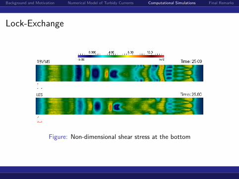
Lock-Exchange

Figure: Non-dimensional shear stress at the bottom


Lock-Exchange

Figure: View of vortical structures, Q-criterium iso-surfaces (Q=0.3).


Lock-Exchange Gr = 9.0× 107

Figure: Top view: shear stress distribution at the bottom


Lock-Exchange ( deposition) Gr = 1.0× 108

Time evolution of the concentration field


Lock-Exchange – Gr = 1.0× 108

Figure: Deposit profile at the middle plane: t=25 (left) and t=50 (right)


Lock-Exchange – Gr = 1.0× 108

Figure: Depositon map profile (left) and mass along time (right),comparison among experiments and numerical simulations


Subgrid Modeling


Sustained Flow and Complex Bottom Topography(prelimarly results)


POLYDISPERSE FLOWS


Polydisperse flow: Coarse 80% and Fine 20%

Figure: Depositon map profile (left) and mass along time (right),comparison among experiments and numerical simulations

Ref.: M.M. Nasr-Azadani, B.Hall, E.Meiburg. Polydisperse turbidity currents propagating over complext opography:

Comparison of experimental and depth-resolvedsimulation results. Computer & Geosciences (53), 141 – 153, 2013.


Tank Configuration – Gr = 1.0× 108 (prelimarly results)


ALE (FSI) FORMULATION FOR MORPHODYNAMICS


UNCERTAINTY QUANTIFICATION


General Aspects

Model uncertainty (epistemic), numerical errors, uncertaintyin parameters (initial conditions,physical constants...), all ofthem interacting and compromising the simulations reliabilityVerification and Validation (V&V) and UncertaintyQuantification (UQ)Probabilistic Perspective : parameters modeled as randomvariables or fields. Looking for a PDF instead of a pointsolutionGoverning Equations represented by Stochastic PartialDifferential Equations


Mathematical Preliminaries

To quantify the uncertainty in a system of differential equations weadopt a probabilistic approach.

Definition: Complete probability space (Ω,F ,P)

Ω is a event space,F ⊂ 2Ω is the σ-algebra of subsets in Ω

P : F → [0, 1] is the probability measure

In this framework, the uncertainty in a model is introduced byrepresenting the input data (parameters,geometry,boundary andinitial condition) as random fields.


Mathematical Preliminaries

For a general differential equation defined on D ⊂ Rd , d = 1, 2, 3with boundary ∂D. The problem consists on find a stochasticfunction, u ≡ u(ω, x) : Ω×D −→ R, such that, for everywhereω ∈ Ω, (Main idea: uncertainty as an extra stochastic dimension)

Governing Stochastic Equations

L(ω, x; u) = f (ω, x) x ∈ DB(ω, x; u) = g(ω, x) x ∈ ∂D

with x = (x1, . . . , xd ) ∈ Rd , d ≥ 1, the space coordinates.


Numerical methods

Intrusive Methods

Polynomial Chaos + Galerkin Formulation

Non-Intrusive Methods

Sampling: Monte Carlo, Quasi MC, LHS

Stochastic Collocation : Polynomial Chaos, Quadratures orPolynomial interpolation

Bayesian Surrogates and Gaussian Process Modeling


Scientific Workflows supporting High PerformanceComputing

Scientific/Engineering Computational Experiments Modeledas Scientific Workflows

Simulations generate a lot of data: understanding how tomanage and query simulation data in runtime

Track who performed the computational experiment and whois responsible for its results Provenance data is automaticallyregistered by SWfMS


Provenance

Nodes with 8 cores

Mesh

Processing

Domain

Partitioning

Parallel CFD

SolverInput Meshi

Meshi

partitioned

in M parts

node-x node-x node-x

node-z

./edgeCFDMeshmpirun –n 8

edgeCFDPre

mpirun –n M

edgeCFD

16 Meshi partitions

Solver executed

with 16 cores for

case i

Sample

i

Chiron is running in each core of each node:managing scheduling,fault-tolerance, provenance data gathering

Typical queries : check for convergence of the deterministic solver ;computation on the fly of high order statistics (two point correlation

represents important QoI)for checking convergence regarding stochasticcomponents


Edge-CFD + CHIRON : Two level paralelism

Mesh ProcessingDomain

Partitioning

Parallel CFD

SolverInput Mesh1

Mesh1 partitioned

in M parts

node-01 node-01 node-01

node-02

./edgeCFDMesh mpirun –n 8 edgeCFDPre mpirun –n M edgeCFD

Nodes with 8 cores 16 Mesh1 partitions

Solver executed with 16

cores for each sample

Mesh ProcessingDomain

PartitioningParallel CFD Solver

Input Mesh2Mesh2 partitioned in

M parts

node-03 node-03 node-03

node-04

./edgeCFDMesh mpirun –n M edgeCFD

Nodes with 8 cores 16 Mesh2 partitions

Sample

1

Sample

2

Sample

NMesh Processing

Domain

PartitioningParallel CFD Solver

Input MeshNMeshN partitioned

in M parts

node-X node--X node-X

node-Z

./edgeCFDMesh mpirun –n M edgeCFD

Nodes with 8 cores 16 MeshN partitions

…

N samples (collocation points)

processed in parallel

mpirun –n 8 edgeCFDPre

mpirun –n 8 edgeCFDPre


Proof of Concept Prototype (ongoing research and implementation)

Non-intrusive UQ strategies : Edge-CFD not to be recoded

Stochastic Collocation : low stochastic dimension

Double level parallelization: exploring the stochastic space ;exploring built-in parallel Edge-CFD features

Still more: space-time-stochastic adaptivity (provenance dataand online queries); computing solution statistics(post-processing)Uncertainty on the initial conditions (initial scenario of thecurrents – Lesshaff et al. . Towards inverse modeling of turbiditycurrents: The inverse lock-exchange problem. Computer &Geosciences, 37(4): 521-529,2011 ) and on settling velocity


Lock Exchange ConfigurationGr = 2.5x106 and 320,000 tetrahedra

Example 1: Homogeneous uncertain initial condition – c = c + σcφ with mean and variance given by

(c, σc ) = (1, 0.2). No sediments deposition (uS = 0)

Example 2 :Non uniform initial condition c(x, y, 0;φ) :c(x, y, φ) = c0 +∑2

1φn√

λnfn(x, y), where

λn =4η1η2σ

2Y

[η21 (w(1)

i )2+1][η22 (w(2)

j )2+1]with (η2w2 − 1)s(wL) = 2ηwc(wL) and

fn(x) = 1√(η2w2

n +1)L/2+η

[ηwncos(wnx) + sin(wnx)]. The random variables φ with support [-1,1] are assumed

independent and uniformly distributed.


Uncertainty Propagation - Homogeneous Initial Conditions


Propagation of uncertainties in the QoIs: deposition map


Multipoint Statistics – Spatial Correlation


Final Remarks and Next Steps

RB-VMS as LES model for Tubridity Currents. Room forimprovement in the subrgrid modeling

FSI - ALE formulation for handling bed form evolution

We have made progress on exploring Chiron ( ScientificWorkflow Management Systems) capabilities for UQ analysis -two level paralelism and first steps towards adaptivity. Moreto come.

Characterization of c(x , 0) through inverse stochasticalgorithms (again Chiron has a role to play)


Future Trends

Bayesian Analysis of Turbidity Currents Deposition


A question raised by a geologist

Imaginemos que no eixo do escoamento, ao longo da linha central, exista um poco (posicao XX). A cerca de 1139metros afastado dele, existe um outro poco (posicao YY), conforme o esquema abaixo. O poco na posicao YY estamais alto cerca de 90m em relacao ao poco XX.A pergunta e a seguinte. Uma corrente, entrando pelo eixo, vai depositar na posicao XX. Essa mesma corrente temcondicoes de depositar tambem na posicao YY, apesar do mesmo estar mais alto ??

Penso que poderıamos variar o numero de Reynolds dessa corrente, e ver se em alguma condicao, ela consegue deixarsedimento no poco mais alto.

Isso teria um grande interesse, pois nos ajudaria a entender se as areias que observamos nos dois pocos tem algumachance de estarem conectadas, uma informacao muito relevante para o desenvolvimento dessa area.


A response (in elaboration)...

Integrating (well log from XX) data with the numerical model

Robust predictions relying upon taking into considerationuncertainties (measurements + numerical inputs)

Probabilistic framework: odds to reach YY translated into jointprobabilities (p(DXX ,DYY ) )

Flow driven by spatial distribution in the begining of the flow (initial conditions (scenario). It isnot known!! Inversion (quite expensive).

Initial conditions modeled as random (uncertain) fields (sensitivity analysis) - UncertaintyQuantification

Different scenarios must be analyzed. Physical experiments would help a lot.

Results might be (easly) integrated in a decision making framework (risk analysis)


Bayesian Analysis Framework

Stochastic framework - parameters or (and) physical quantities aremodeled as random variables (fields).

Physics - based models phrased as stochastic partial differential equa-tions (SPDE).

Bayesian techniques emerging as leading tools for analysis

Analysis Bayesian workflow ( inspired in Bayesian modeling of air-sea interaction. Berliner et.

al., Journal of Geophysical Research, 2003.)

πpost := π(D,m|d) ∝ [d|D] L(D|m) πprior (m) (2)d ... well log data : deposits heights and sediments distribution.m . . . initial conditions (initial scneario) and settling velocity

[d|D] ... data model (measurments errors)

L (likelihood) . . containing the forward model (or a computational surrogate)


Analysis

Equation (2) is often not amenable to be treated by analytcalmeans

Indeed, one might want only to compute quantiles...P(Dj ≤ D) or analyse plausible scnearios. Sampling will do.

Sampling from πpost is not a trivial task... Markov ChainMonte Carlo algorithms represent a good option. But theywill be quite expensive (a forward problem is to be solved foreach sample (accpeted or not)

Computational Surrogates :I.Bilionis, N. Zabaras, B. A. Konomi, G. Lin. Multi-output

separable Gaussian process: Towards an efficient fully Bayesian paradigm for uncertainty quantitication.

Journal of Computational Physics 241 (2013) 212–239.

a variational multiscale large eddy computational...

Documents