variational multiscale residual-based turbulence modeling ...€¦ · variational multiscale...
TRANSCRIPT

Available online at www.sciencedirect.com
www.elsevier.com/locate/cma
Comput. Methods Appl. Mech. Engrg. 197 (2007) 173–201
Variational multiscale residual-based turbulence modeling forlarge eddy simulation of incompressible flows
Y. Bazilevs a,*, V.M. Calo a, J.A. Cottrell a, T.J.R. Hughes a,1, A. Reali b, G. Scovazzi c,2
a Institute for Computational Engineering and Sciences, The University of Texas at Austin, 201 East 24th Street,
1 University Station C0200, Austin, TX 78712, USAb Structural Mechanics Department, University of Pavia, via Ferrata 1, 27100 Pavia, Italy
c 1431 Computational Shock and Multi-physics Department, Sandia National Laboratories, P.O. Box 5800, MS 1319, Albuquerque, NM 87185-1319, USA
Received 2 May 2007; received in revised form 5 July 2007; accepted 19 July 2007Available online 15 August 2007
Abstract
We present an LES-type variational multiscale theory of turbulence. Our approach derives completely from the incompressibleNavier–Stokes equations and does not employ any ad hoc devices, such as eddy viscosities. We tested the formulation on forced homo-geneous isotropic turbulence and turbulent channel flows. In the calculations, we employed linear, quadratic and cubic NURBS. A dis-persion analysis of simple model problems revealed NURBS elements to be superior to classical finite elements in approximatingadvective and diffusive processes, which play a significant role in turbulence computations. The numerical results are very good and con-firm the viability of the theoretical framework.� 2007 Elsevier B.V. All rights reserved.
Keywords: Variational multiscale methods; Large eddy simulation; Turbulence modeling; Optimality; Projection; Small-scale Green’s function; Pertur-bation series; Isogeometric analysis; NURBS; Incompressible flows; Homogeneous isotropic turbulence; Turbulent channel flows
1. Introduction
Variational multiscale concepts for Large Eddy Simula-tion (LES) were introduced in [33]. The basic idea was touse variational projections in place of the traditional filteredequations and to focus modeling on the fine-scale equa-tions. Avoidance of filters eliminates many difficultiesassociated with the traditional approach, namely, inhomo-geneous non-commutative filters necessary for wall-bounded flows, use of complex filtered quantities incompressible flows, etc. In addition, modeling confined to
0045-7825/$ - see front matter � 2007 Elsevier B.V. All rights reserved.
doi:10.1016/j.cma.2007.07.016
* Corresponding author.E-mail address: [email protected] (Y. Bazilevs).
1 Aerospace Engineering and Engineering Mechanics, Computationaland Applied Mathematics Chair III.
2 Sandia is a Multiprogram Laboratory Operated by Sandia Corpora-tion, a Lockheed Martin Company, for the United States Department ofEnergy’s National Nuclear Security Administration under Contract DE-AC04-94-AL85000.
the fine-scale equations retains numerical consistency inthe coarse-scale equations and thus permits full rate-of-convergence of the underlying numerical method in con-trast with the usual approach, which limits convergence ratedue to artificial viscosity effects in the fully resolved scales(O(h4/3) in the case of Smagorinsky-type models). Initialversions of the variational multiscale method focused ondividing resolved scales into coarse and fine designations,and eddy viscosities, inspired by traditional models, wereonly included in the fine-scale equations, and acted onlyon the fine scales. This version was studied in [34,36,56],and found to work very well on homogeneous isotropicflows and fully-developed equilibrium and non-equilibriumturbulent channel flows. Static eddy viscosity modelswere employed in these studies but superior results weresubsequently obtained through the use of dynamic models,as reported in [27,41]. Good numerical results wereobtained with the static approach by other investigators,namely, Collis [18], Jeanmart and Winckelmans [44], and
174 Y. Bazilevs et al. / Comput. Methods Appl. Mech. Engrg. 197 (2007) 173–201
Ramakrishnan and Collis [59–62]. Particular mentionshould be made of the work of Farhat and Koobus [20],and Koobus and Farhat [48], who have implemented thisprocedure in an unstructured mesh, finite element/finite vol-ume, compressible flow code, and applied it very success-fully to a number of complex test cases and industrialflows. A valuable review with many references to relevantliterature may be found in [22]. We believe that this initialversion of the variational multiscale concept has alreadydemonstrated its viability and practical utility and is, atthe very least, competitive with traditional LES turbulencemodeling approaches. For a comprehensive treatment ofmultiscale concepts in turbulence, see [65]. There has alsobeen a number of contributions to the literature in whichstabilized numerical methods have been used to model tur-bulence (see, e.g. [26]). These endeavors are somewhat dif-ferent in philosophy than the present contribution.
Nevertheless, there is still significant room for improve-ment. The use of traditional eddy viscosities to representfine-scale dissipation is an inefficient mechanism. Employ-ing an eddy viscosity in the resolved fine scales to representturbulent dissipation introduces a consistency error, whichresults in the resolved fine scales being sacrificed to retainfull consistency in the coarse scales. (In our opinion, thisis still better than the traditional approach in which consis-tency in all resolved scales is sacrificed to represent turbu-lent dissipation.) This procedure is felt to be inefficientbecause approximately 7/8 of the resolved scales are typi-cally ascribed to the fine scales. Another shortcomingnoted for the initial version of the variational multiscalemethod is too small an energy transfer to unresolved modeswhen the discretization is very coarse (see, e.g. [41]). Thisphenomenon is also noted for some traditional models,such as the dynamic Smagorinsky model, Hughes et al.[41], but, by design, is more pronounced for the multiscaleversion of the dynamic model. The objectives of recent mul-
tiscale work have been to capture all scales consistently and
to avoid use of eddy viscosities altogether. This holds thepromise of much more accurate and efficient LES proce-dures. In this work, we describe a new variational multi-scale formulation, which makes considerable progresstoward these goals. In what follows, all resolved scalesare viewed as coarse scales, which obviates the aforemen-tioned issue of inefficiency ab initio.
We begin by taking the view that the decomposition intocoarse and fine scales is exact. For example, in the spectralcase, the coarse-scale space consists of all Fourier modesbeneath some cut-off wave number and the fine-scale spaceconsists of all remaining Fourier modes. Consequently, thecoarse-scale space has finite dimension whereas the fine-scale space is infinite dimensional. The derivation of thecoarse- and fine-scale equations proceeds, first, by substi-tuting the split of the exact solution into coarse and finescales into the Navier–Stokes equations, then, second, byprojecting this equation into the coarse- and fine-scale sub-spaces. The projection into coarse scales is a finite-dimen-sional system for the coarse-scale component of the
solution, which depends parametrically on the fine-scalecomponent. In the spectral case, in addition to the usualterms involving the coarse-scale component, only thecross-stress and Reynolds-stress terms involve the fine-scalecomponent. In the case of non-orthogonal bases, even thelinear terms give rise to coupling between coarse and finescales. The coarse-scale component plays an analogous roleto the filtered field in the classical approach, but has theadvantage of avoiding all problems associated with homo-geneity, commutativity, walls, compressibility, etc. Theprojection into fine scales is an infinite-dimensional systemfor the fine-scale component of the solution, which dependsparametrically on the coarse-scale component. We alsoassume the cut-off wave number is sufficiently large thatthe philosophy of LES is appropriate. For example, if thereis a well-defined inertial sub-range, then we assume the cut-off wave number resides somewhere within it. This assump-tion enables us to further assume that the energy content inthe fine scales is small compared with the coarse scales.This turns out to be important in our efforts to analyticallyrepresent the solution of the fine-scale equations. The strat-egy is to obtain approximate analytical expressions for thefine scales then substitute them into the coarse-scale equa-tions which are, in turn, solved numerically. If the scaledecomposition is performed in space and time, the only
approximation in the procedure is the representation ofthe fine-scale solution. To provide a framework for thefine-scale approximation, we assume an infinite perturba-tion series expansion to treat the fine-scale nonlinear termin the fine-scale equation. By virtue of the smallness ofthe fine scales, this expansion is expected to converge rap-idly under the circumstances described in many cases ofpractical interest. The remaining part of the fine-scaleNavier–Stokes system is the linearized operator which isformally inverted through the use of a matrix Green’s func-tion. The combination of a perturbation series and Green’sfunction provides an exact formal solution of the fine-scaleNavier–Stokes equations. The driving force in these equa-tions is the Navier–Stokes system residual computed fromthe coarse scales. This expresses the intuitively obvious factthat if the coarse scales constitute a good approximation tothe solution of the problem, the coarse-scale residual willbe small and the resulting fine-scale solution will be smallas well. This is the case we have in mind and it providesa rational basis for assuming the perturbation series con-verges rapidly. Note that one cannot use such an argumenton the original problem because in this case the perturba-tion series would almost definitely fail to converge. (If wecould have used this argument, we would have solved theNavier–Stokes equations analytically! Unfortunately, itdoes not work.) The formal solution of the fine-scale equa-tions suggests various approximations may be employed inpractical problem solving. We are tempted to use the word‘‘modeling’’ because approximate analytical representa-tions of the fine scales constitute the only approximationand hence may be thought of as the ‘‘modeling’’ compo-nent of the present approach but we want to emphasize

Fig. 1. Space-time domain (left) and slicing into space-time slabs (right).
Y. Bazilevs et al. / Comput. Methods Appl. Mech. Engrg. 197 (2007) 173–201 175
that it is very different from classical modeling ideas whichare dominated by the addition of ad hoc eddy viscosities.We will present numerical results that demonstrate theseeddy viscosity terms are unnecessary in the present circum-stances. There are two aspects to the approximation of thefine scales: (1) approximation of the matrix Green’s func-tion for the linearized Navier–Stokes system and (2)approximation of the nonlinearities represented by theperturbation series. The first and obvious thought forthe latter aspect, nonlinearity, is to simply truncate theperturbation series. This idea is investigated, as well asanother promising idea, in conjunction with some simpleapproximations of the Green’s function. It turns out thereis considerable experience in local scaling approximationsof the Green’s function based on the theory of stabilizedmethods [28,31,39]. These ideas derive inspiration fromthe asymptotic approaches of Barenblatt [2]. The Green’sfunction is typically approximated by locally defined alge-braic operators (i.e., the ‘‘s’s’’ of stabilized methods) multi-plied by local values of the coarse-scale residual. With thisapproximation of the solution of the linearized operator,nonlinearities can be easily accounted for in perturbationseries fashion.
The remainder of the paper is summarized as follows: InSection 2 we present the mathematical details of the varia-tional multiscale theory described previously. This repre-sents our general approach to LES-style turbulencemodeling and is independent of the specifics of the discretespaces utilized to represent the coarse scales. In Section 3,we present ideas supporting the use of simplified scalingarguments to represent the fine scales. In Section 4, wedescribe the implementational aspects of the proceduresused herein and the details of the fine-scale approximation.The relationship between this version of the variational mul-tiscale method and classical stabilized methods is delineated.The variational multiscale method includes additionalterms. Both conceptually and from the point of view ofactual implementation, stabilized methods may be viewedas historical stepping stones leading to the more coherentvariational multiscale formulation. In Section 5, the timeintegration techniques are presented. In Section 6, we pres-ent our numerical studies of forced isotropic turbulence atRek = 165 and Rek =1. (Rek is the Taylor microscale Rey-nolds number.) We begin in Section 6.1 with a description ofthe approximation spaces consisting of NURBS elements(non-uniform rational B-splines, see, e.g. [63,57,21,17]). Inthe case of the rectilinear geometry considered, NURBSreduce to B-splines, which have been advocated for turbu-lence calculations previously (see [49,68,50,51]). We employtrivariate linear, quadratic, and cubic NURBS with periodicboundary conditions. Linear trivariate NURBS turn out tobe identical to trilinear hexahedral finite elements, but thehigher-order NURBS are different than classical higher-order finite elements. In Section 6.2, we perform a dispersionerror analysis for NURBS versus classical finite elements onsimple, linear, one-dimensional advective and diffusivemodel problems, and conclude that NURBS have better
approximation properties than classical finite elements. InSection 6.3, we describe the way we force the turbulenceand in Section 6.4 we present the results of our numericalcalculations. We employ meshes of 323, 643, 1283, and2563 to explore convergence with mesh refinement (h-con-vergence) and we examine the behavior of increasing orderfrom linear to cubic on fixed meshes (k-convergence). Inthe case of Rek = 165, we compare with the DNS spectralresults of Langford and Moser [52]. Energy spectra andthird-order structure functions are presented. Our assess-ment is that the results are very good for all cases. In the caseof Rek =1 we can clearly see the development of an inertialsubrange. In Section 7 we present results for turbulent chan-nel flows at Res = 395. (Res is the wall-friction Reynoldsnumber.) We employ meshes of 323 and 643. This time themesh is graded in the wall-normal direction to better capturethe boundary layer. Again, we consider convergence fromthe h- and k-refinement perspectives. A striking result ishow much better quadratic elements are than linear ele-ments. For a mesh of 643, the quadratic and cubic resultsare essentially identical to the DNS results of Moser et al.[55] for first- and second-order statistics, and for a mesh of323 they are in close agreement. Conclusions are drawn inSection 8.
2. Variational multiscale formulation of the incompressible
Navier–Stokes equations
In this section we describe our turbulence modelingtheory.
2.1. Incompressible Navier–Stokes equations
We consider a space-time domain Q ¼ X��0; T ½�R3 � Rþ with lateral boundary P = C·]0, T[, as illustratedin the left-hand side of Fig. 1. The initial/boundary-valueproblem consists of solving the following equations foru : Q! R3, the velocity, and p : Q! R, the pressure(divided by the constant density),

176 Y. Bazilevs et al. / Comput. Methods Appl. Mech. Engrg. 197 (2007) 173–201
ou
otþr � ðu� uÞ þ rp ¼ mDuþ f in Q; ð1Þ
r � u ¼ 0 in Q; ð2Þu ¼ 0 on P; ð3Þuð0þÞ ¼ uð0�Þ on X; ð4Þ
where f : Q! Rd is the given body force (per unit volume);m is the kinematic viscosity, assumed positive and constant;uð0�Þ : X! Rd is the given initial velocity; and � denotesthe tensor product (e.g., in component notation,[u � v]ij = uivj).
Eqs. (1)–(4) are, respectively, the linear momentum bal-ance, the incompressibility constraint, the no-slip boundarycondition and the initial condition.
2.1.1. Global space-time variational formulation
Let V ¼VðQÞ denote both the trial solution andweighting function spaces, which are assumed to be identi-cal. We assume U ¼ fu; pg 2V implies u = 0 on P andR
X pðtÞdX ¼ 0 for all t2]0, T[. Let (Æ, Æ)x denote the L2 innerproduct with respect to the domain x. The variational for-mulation is stated as follows:
Find U 2V such that 8W ¼ fw; qg 2V:
BðW ;UÞ ¼ B1ðW ;UÞ þ B2ðW ;U ;UÞ ¼ LðWÞ ð5Þ
with
B1ðW ;UÞ ¼ ðwðT�Þ; uðT�ÞÞX �ow
ot; u
� �Q
;
þ ðq;$ � uÞQ � ð$ � w; pÞQ þ $sw; 2m$suð ÞQ;ð6Þ
B2ðW ;U ;VÞ ¼ � $w; u� vð ÞQ; ð7ÞLðWÞ ¼ ðw; f ÞQ þ ðwð0
þÞ; uð0�ÞÞX; ð8Þ
where V = {v, Æ} and $su ¼ ð$uþ ð$uÞT Þ=2. Note thatB1(Æ, Æ) is a bilinear form and B2(Æ, Æ, Æ) is a trilinear form.Assuming sufficient regularity and integrating by parts,we obtain the Euler–Lagrange form of (5)–(8):
0 ¼ w;ou
otþ $ � ðu� uÞ þ $p � $ � 2m$su� f
� �Q
þ q;$ � uð ÞQ þ ðwð0þÞ; uð0þÞ � uð0�ÞÞX ð9Þ
which reveals that the variational formulation implies satis-faction of the momentum equations, incompressibility con-straint, and initial condition. The velocity boundarycondition is built into the definition of the space V. In sum-mary, the variational formulation is equivalent to (1)–(4).
3 The way U is determined from U is a very important issue, and it hasvery significant impact on the theory to be developed. An initiatory studyof typical projectors is presented in [37]. Not only can one envision aninfinite number of possible projectors, but one can also envision an infinitenumber of nonlinear optimization schemes that ‘‘fit’’ U to U. In someapplications nonlinear schemes will surely be important, an example beingcompressible turbulence with shocks where monotonicity is important.However, for incompressible turbulence, we feel linear projectors, such asthe H1-projector, should suffice. (See [35] for an application of the H1-projector in turbulence.)
2.1.2. Sliced space-time variational formulation
Consider a slicing of space-time obtained by replacing]0,T[ by ]tn, tn+1[, n = 0,1,2, . . .,N, and summing over thespace-time slabs Qn (see Fig. 1). The counterparts of (5)–(9) for a typical slab are:
BðW ;UÞn ¼ B1ðW ;UÞn þ B2ðW ;U ;UÞn ¼ LðWÞn; ð10Þ
B1ðW ;UÞn ¼ ðwðt�nþ1Þ; uðt�nþ1ÞÞX �ow
ot; u
� �Qn
þ ðq;$ � uÞQn� ð$ � w; pÞQn
þ $sw; 2m$suð ÞQn;
ð11ÞB2ðW ;U ;VÞn ¼ � $w; u� vð ÞQn
; ð12ÞLðWÞn ¼ ðw; f ÞQn
þ ðwðtþn Þ; uðt�n ÞÞX; ð13Þ
0 ¼ w;ou
otþ $ � ðu� uÞ þ $p � $ � 2m$su� f
� �Qn
þ q;$ � uð ÞQnþ ðwðtþn Þ; uðtþn Þ � uðt�n ÞÞX; ð14Þ
where in (10)–(14), U = {u, p} and W = {w, q} belong toVn ¼VðQnÞ, the restriction of V to Qn. From the Eu-ler–Lagrange form of the equation, (14), we see that themomentum equation and incompressibility constraint aresatisfied on the slab, and the solution is continuous acrossslab interfaces. The formulation in terms of space-timeslabs exploits the causal nature of the Navier–Stokes equa-tions and reduces the overall problem to a succession of ini-tial/boundary-value problems on the slabs. The solution isobtained solving the variational equation on each slab suc-cessively, n = 0,1,2, . . .,N. We emphasize that this is an ex-
act formulation, entirely equivalent to (5)–(9), and (1)–(4).However, it is a more suitable starting point for the devel-opment of numerical schemes.
Remark
In order to simplify notation in the sequel, we will workwith the global form of the variational equation. However,all results are equally applicable to the variational equa-tions of the individual space-time slabs.
2.2. Scale separation
We consider a direct-sum decomposition of V into‘‘coarse-scale’’ and ‘‘fine-scale’’ subspaces, V and V0,respectively,
V ¼V�V0: ð15Þ
V is assumed to be a finite-dimensional space and it will beidentified later with the space of functions with which weactually compute. In order to make the decomposition welldefined, we need to introduce a procedure for uniquelydetermining U 2V and U 0 2V0 from a given U 2V.This can be accomplished with the aid of a projectorP : V!V. For example, P could be the L2-projector,H1-projector, etc. There are infinitely many possibilities.3

Y. Bazilevs et al. / Comput. Methods Appl. Mech. Engrg. 197 (2007) 173–201 177
Once P is selected, we know how the coarse scales approx-imate all scales, viz.,
U ¼ PU ; ð16ÞU 0 ¼ U � PU ¼ ðI� PÞU ; ð17Þ
where I is the identity operator. Likewise, we can decom-pose a weighting function into its coarse- and fine-scalecomponents:
W ¼ PW ; ð18ÞW 0 ¼W � PW ¼ ðI� PÞW : ð19Þ
With these, we may decompose the original variationalequation into coupled coarse-scale and fine-scale equa-tions, viz.,
BðW ;U þU 0Þ ¼ LðWÞ; ð20ÞBðW 0;U þU 0Þ ¼ LðW 0Þ; ð21Þ
where
BðW ;U þU 0Þ ¼ B1ðW ;UÞ þ B1ðW ;U 0Þþ B2ðW ;U ;UÞ þ B2ðW ;U ;U 0Þþ B2ðW ;U 0;UÞ þ B2ðW ;U 0;U 0Þ; ð22Þ
BðW 0;U þU 0Þ ¼ B1ðW 0;UÞ þ B1ðW 0;U 0Þþ B2ðW 0;U ;UÞ þ B2ðW 0;U ;U 0Þþ B2ðW 0;U 0;UÞ þ B2ðW 0;U 0;U 0Þ: ð23Þ
In (22), B2ðW ;U ;U 0Þ and B2ðW ;U 0;UÞ correspond to thecross-stress terms, and B2ðW ;U 0;U 0Þ corresponds to theReynolds stress term. Eq. (21) can be expressed as
BUðW0;U 0Þ þ B2ðW 0;U 0;U 0Þ ¼ hW 0;ResðUÞiV0 ;V0 ; ð24Þ
where
BUðW0;U 0Þ ¼B1ðW 0;U 0ÞþB2ðW 0;U 0;UÞþB2ðW 0;U ;U 0Þ ð25Þ
hW 0;ResðUÞiV0 ;V0 ¼ LðW 0Þ�B1ðW 0;UÞ�B2ðW 0;U ;UÞ ð26Þ
in which ResðUÞ is the coarse-scale residual ‘‘lifted’’ to thedual of the fine-scale space V0, h�; �iV0;V0 is the dualitypairing, and
BUð�;U0Þ ¼ d
deBð�;U þ eU 0Þ
� �e¼0
ð27Þ
Fig. 2. The variational multiscale turbulence modeling theory is schematicallysubstituted into the coarse-scale equation. The coarse scales are the representeintroduced.
the linearization of Bð�;U þU 0Þ about U in the directionU 0. Note that the solution of (24) can be formally repre-sented as a functional of U and ResðUÞ, namely,
U 0 ¼ F 0ðU ;ResðUÞÞ ð28Þ
The explicit dependence on U in the first argument of F 0
emanates from the dependence of the linearized operatorBU on U . This expression can be inserted into (20) to‘‘close’’ the finite-dimensional system for U ,
B W ;U þ F 0ðU ;ResðUÞÞ� �
¼ LðWÞ ð29Þ
Eqs. (28) and (29) can be thought of in global terms or interms of a sequence of space-time slabs. In both cases, theyrepresent a procedure for solving the Navier–Stokes equa-tions in terms of a scale decomposition of the solution. Sofar we have not discussed approximations or numerics. Thesolution U ¼ U þU 0, where U is determined by solving(29) and U 0 is determined from U through (28), is the exact
solution of the original variational problem, (20) and (21),and (1)–(4), the Navier–Stokes initial/boundary-valueproblem.
Our plan for turbulence modeling is to systematicallyapproximate the functional F 0. This will provide us with aparameterization of the fine scales in terms of the coarsescales, which can be substituted in the coarse-scale equa-tion, ‘‘closing’’ it. The finite-dimensional coarse-scale equa-tion can then be solved. In this way we obtain anapproximate coarse-scale solution and an estimation ofthe fine scales. In summary, our variational multiscale the-ory of turbulence modeling is encapsulated in the followingequations:
eU 0 ¼ eF 0ð eU ;Resð eU ÞÞ ð30Þ
BðW ; eU þ eF 0ð eU ;Resð eU ÞÞÞ ¼ LðWÞ ð31Þ
where eF 0 is an approximation of the exact functional F 0,and eU 0 and eU are the approximations of U 0 and U , respec-tively. The concept underlying the model is illustrated inFig. 2. We also note that (30) constitutes an a posteriori
estimation of the error in the coarse-scale solution (see[31,39,24,25]).
illustrated. The fine, or ‘‘subgrid’’ scales are solved for analytically andd scales in a calculation. Note that there is no ad hoc eddy viscosity model

178 Y. Bazilevs et al. / Comput. Methods Appl. Mech. Engrg. 197 (2007) 173–201
Remarks
(1) (31) may be thought of as playing a similar role in thevariational multiscale theory as the filtered equationsplay in traditional turbulence modeling. Distinguish-ing features are (31) is finite-dimensional and closed,in contrast with the filtered equations.
(2) Intuitively, the ‘‘better’’ the fine-scale approximation,the smaller the dimension of the coarse-scale spacerequired, and consequently, the smaller the computa-tional effort. It is also possible to envision a hierarchyof approximations that produce variational multi-scale analogues of traditional turbulence modelingconcepts, such as large eddy simulation (LES),detached eddy simulation (DES), and the Reynoldsaveraged Navier–Stokes (RANS) approach. LES rep-resents the turbulence modeling methodology requir-ing the greatest computational burden, but perhapsthe least complex modeling. In the following sectionswe will endeavor to develop a variational multiscaleanalogue of LES within the theoretical frameworkof (30) and (31).
(3) It is very important to emphasize that in practice wework directly with (31), a finite-dimensional system,and we consider the solution of (31), eU , our approx-imation to U , and in turn our approximation to U.Recall, by design of P, U is an approximation to U.We do not need to solve for the fine scales andbecause of this (30) is completely extraneous, unlesswe wish to use it to estimate the error in the coarsescales. That being said, it may also be interesting toconsider eU þ eU 0 as an alternative approximation toU. It will of course be necessary to assume that thecoarse-scale space is sufficiently large for the philoso-phy of LES to be appropriate. That is, if there is awell-defined inertial subrange, then we assume thecut-off between the coarse- and fine-scale spacesresides somewhere within it. This assumption enablesus to further assume that the energy content in thefine scales is small compared with the coarse scales,an aspect of considerable importance in attemptingto analytically determine the solution of the fine-scaleequations.
2.3. Perturbation series
It seems reasonable to assume that the larger the spaceV, the better the approximation of U to U, and the smallerthe coarse-scale residual ResðUÞ 2V0. We further assumethat if ResðUÞ ¼ 0, then F 0ðU ; 0Þ ¼ 0, and if ResðUÞ is‘‘small’’, then U 0 will likewise be ‘‘small’’.4 These assump-tions suggest a perturbation series expansion of the form:
4 These assumptions seem physically reasonable, but rigorous mathe-matical justification may be difficult to obtain. The existence of non-trivial,unforced weak solutions of the Euler equations, compact in space andtime, underscores the mathematical difficulties of the Navier–Stokesequations at large Reynolds numbers (see [69]).
U 0 ¼ eU 01 þ e2U 02 þ e3U 03 þ � � � ¼X1k¼1
ekU 0k; ð32Þ
where e ¼ kResðUÞkV0 . Let us rewrite (24) in terms of theproposed expansion:
BU W 0;X1k¼1
ekU 0k
!þ B2 W 0;
X1k¼1
ekU 0k;X1k¼1
ekU 0k
!¼ ehW 0; bRðUÞi ð33Þ
where h�; �i ¼ h�; �iV0;V0 , and
bRðUÞ ¼ ResðUÞResðUÞ�� ��
V0
: ð34Þ
Notice that, by linearity,
BU W 0;X1k¼1
ekU 0k
!¼X1k¼1
ekBUðW0;U 0kÞ; ð35Þ
while the second term requires further consideration. Weexpand it as follows:
B2ðW 0; eU 01 þ e2U 02 þ e3U 03 þ � � � ; eU 01 þ e2U 02 þ e3U 03 þ � � �Þ¼ e2B2 W 0;U 01;U
01
� �þ e3 B2 W 0;U 01;U
02
� ��þ B2 W 0;U 02;U
01
� ��þ e4 B2 W 0;U 01;U
03
� ��þ B2 W 0;U 02;U
02
� �þ B2 W 0;U 03;U
01
� ��þ � � � ð36Þ
A recurrence formula can be easily deduced, by groupingcoefficients of the powers of e:
e2 ! B2ðW 0;U 01;U01Þ;
e3 ! B2 W 0;U 01;U02
� �þ B2 W 0;U 02;U
01
� �;
e4 ! B2 W 0;U 01;U03
� �þ B2 W 0;U 02;U
02
� �þ B2 W 0;U 03;U
01
� �;
e5 ! � � � þ � � � þ � � � þ � � �
Hence
B2 W 0;X1k¼1
ekU 0k;X1k¼1
ekU 0k
!¼X1k¼2
ekXk�1
j¼1
B2ðW 0;U 0j;U0k�jÞ:
ð37Þ
The full expansion of the equation can be compactly writ-ten asX1k¼1
ekBUðW0;U 0kÞ þ
X1k¼2
ekXk�1
j¼1
B2ðW 0;U 0j;U0k�jÞ
¼ ehW 0; bRðUÞi: ð38Þ
Equating like coefficients, we obtain a sequence of linearvariational problems coupled through their right-handsides:
For k ¼ 1 BU W 0;U 01� �
¼ hW 0; bRðUÞiV0 ;V0 ; ð39Þ
For k P 2 BU W 0;U 0k� �
¼ �Xk�1
j¼1
B2 W 0;U 0j;U0k�j
: ð40Þ
Y. Bazilevs et al. / Comput. Methods Appl. Mech. Engrg. 197 (2007) 173–201 179
The bilinear operator BUð�; �Þ is the same for all the prob-lems in the cascade, and can be formally inverted througha Green’s operator. The Green’s operator concept can beintroduced in an abstract sense through a resolvent
operator:
G 0Uð�Þ ¼ G 0ðU ; �Þ : V0 !V0; ð41Þ
Fð�Þ7!V 0: ð42Þ
such that
BUðW0;V 0Þ ¼FðW 0Þ: ð43Þ
If a sequence of operators Fj : V0 ! R (i.e., Fj 2V0) isdefined as
For k ¼ 1 F1ðW 0Þ ¼F1ðW 0; bRðUÞÞ¼ hW 0; bRðUÞiV0;V0 ; ð44Þ
For k P 2 FkðW 0Þ ¼FkðW 0; U 01; . . . ;U 0k�1Þ
¼ �Xk�1
j¼1
B2 W 0;U 0j;U0k�j
ð45Þ
then it is possible to reformulate the sequence of problems(39) and (40) as
U 0k ¼ G 0UðFkÞ ¼ G 0ðU ;FkÞ; k ¼ 1; 2; . . . ð46Þ
Notice that in the cascade of problems (39) and (40) (or,equivalently, (44) and (45), or (46)) the level-k term in theexpansion depends on terms on the right-hand side, whichinvolve the coarse-scale residual and terms in the expansionfrom level 1 to k � 1.
Upon substituting the U 0k’s into the series (32), the pow-ers of e ¼ kResðUÞkV0 cancel out. If the series converges, itrepresents an exact solution to the fine-scale equation, andthen (31) gives the exact solution of the coarse-scale equa-tion. In other words, given the validity of the assumptions,the exact solution of the original Navier–Stokes system isobtained. In order to determine the exact solutions of eachof the linear problems in the cascade, we need the exactGreen’s operator G 0
U. This is a non-classical Green’s oper-
ator, referred to as the ‘‘fine-scale Green’s operator,’’ thatin turn depends on the classical Green’s operator and theselected projector P (see [37]):
G 0 ¼ G � GPðPGPÞ�1PG ; ð47Þ
where P is the adjoint of P. Note that the orthogonalityproperties:
PG 0 ¼ 0; ð48ÞG 0P ¼ 0 ð49Þ
immediately follow from (47). In [37] it was shown, in thecontext of finite element approximations of the advec-tion–diffusion equation, for the advection-dominated case,that the projector based on the H 1
0-inner product (termedthe Dirichlet projector in [35]) produced a highly localizedfine-scale Green’s operator, despite the classical Green’soperator being highly non-local. In fact, for the one-dimen-
sional case, the support of the fine-scale Green’s operatorwas confined to individual elements, and there was no cou-pling between elements. It is important to realize that this isnot a general feature of the fine-scale Green’s operator, butone that depends crucially on the particular projector. Forexample, the fine-scale Green’s operator produced by theL2-projector was non-local in all cases.
Exact determination of the Green’s function is not pos-sible and neither is summing an infinite number of terms inthe perturbation series. Consequently, two approximationsare necessary in order to develop a practical solutionscheme:
(1) Approximation of the fine-scale Green’s operator forthe linearized Navier–Stokes system, eG 0
U G 0
U.
(2) Approximation of the nonlinearities by truncation ofthe perturbation series.
Once these approximations are made precise, we havedefined a turbulence model of the form (31). This will bediscussed in the following section.
RemarkIt needs to be emphasized that the pathway to an
approximate turbulence model identified by the aboveassumptions is not the only possibility, but it does seem aviable candidate for LES-type modeling within the varia-tional multiscale method. Clearly, a more direct attackon the fully nonlinear fine-scale equation, rather than theperturbation series approach, might seem an even morepropitious approach. In either case, our theoretical frame-work for turbulence modeling remains (30) and (31).
3. Approximating the fine-scale Green’s operator
A study of the fine-scale Green’s operator for the linear,steady, advection–diffusion equation was performed in [37],in which an explicit formula was derived in terms of theclassical Green’s operator and a projector onto thecoarse-scale space, given here by (47). It was shown thatdifferent projectors yielded very different locality propertiesof the fine-scale Green’s operator. The H 1
0-projector pro-duced a highly localized Green’s operator, whereas theL2-projector exhibited more global support. Locality is avery desirable property because it suggests local approxi-mation, a significant simplification from the practical view-point. It has been known for some time that stabilizationoperators represent local approximations to fine-scaleGreen’s operators (see [28,10,31,37]) and this also suggeststhat the product of stabilization operators and coarse-scaleresiduals would represent very simple but potentially effec-tive representations of fine-scale fields. (A more precise jus-tification of this idea for simple model problems was givenin [37].)
So far, for the most part, effort devoted to calculatingfine-scale Green’s operators has utilized an analyticalapproach. This can only be executed rigorously in thesimplest circumstances (see [28,10,31,37]), but provides

180 Y. Bazilevs et al. / Comput. Methods Appl. Mech. Engrg. 197 (2007) 173–201
valuable insight and serves as a basis for comparing withapproximate and more practically useful procedures. Givena fine-scale basis, and the variational equation for the fine-scale field, the fine-scale Green’s operator can be computed(see [31]). However, heretofore no practical success hasbeen attained with this approach because the functionsused to represent the fine-scale basis, typically low-orderpolynomials, have not been able to faithfully describeadvection-dominated asymptotic behavior, of paramountimportance in high Reynolds and Peclet number applica-tions. Recently, progress has been made by two of us (Cott-rell and Hughes) utilizing the discontinuous variationalmultiscale method (see [38,9,13]). This approach providesconsiderable generality and enables fine-scales fields to becalculated numerically, accounting for nonlinearity, andtime dependence. We believe it will represent an importantstep forward in better representing fine-scale fields, result-ing in more accurate turbulence modeling procedures,and we hope to report on it in the near future.
In the present work we are content to work on the mostsimple and basic end of the approximation spectrum. Theidea is to compute element-wise stabilization operators,denoted s, and calculate the fine-scale field as the productof s and the local coarse-scale residual,
eU 0 �sResð eU Þ: ð50Þ
Note that s is matrix-valued in our case, specifically,s 2 R4�4, and it can be computed from the formula forthe fine-scale Green’s operator by assuming it takes theform of s times a Dirac distribution in each element. Theresult that ensues is that s is the element mean value ofthe fine-scale Green’s operator. In the case of a space-timeelement, Qe
n, we have (see [40])
sjQe ¼ 1
jQej
ZQe
ZQe
eG 0eU
ðx; t; x; tÞdQdQ: ð51Þ
Note that s is a function of eU . This formula has been usedto determine precise values of s for simple cases, primarilyin the steady case, but, more often than not, well-estab-lished asymptotic scaling arguments have been used to di-rectly calculate s in more complex circumstances. Thereare a number of references to this beginning with some ofthe earliest works on stabilized methods (see, e.g.[12,67,72,39,66,14,3]). This is the approach adopted hereand the precise formula utilized is given in the followingsection.
Once we have a formula such as (50) we can constructthe entire perturbation series approximation, as shown in[66,14]. However, in the present work, keeping with thetheme of simplicity, we will truncate the series at the firstterm, namely (50).
Having described the simple path chosen in this work,we do wish to emphasize that we view it as extremelyimportant to investigate other, richer possibilities withinour theoretical framework of the fine-scale problem. Webelieve this will lead to practical and theoretical benefits.
4. Implementation
The space-time formulation of Section 2 is very generaland is suggestive of a wide variety of interpretations. Forfixed spatial domains semi-discrete formulations are veryeconomical (see, e.g. [8]), and this is what is employedherein. In place of (20) and (22), we have, respectively,
BhðWh;Uh þU 0Þ ¼ LhðWhÞ; ð52ÞBhðWh;Uh þU 0Þ ¼ Bh
1ðWh;UhÞ þ Bh2ðWh;Uh;UhÞ þ ~Bh
1ðWh;U 0Þþ Bh
2ðWh;Uh;U 0Þ þ Bh2ðWh;U 0;UhÞ ðCross stressÞ
þ Bh2ðWh;U 0;U 0Þ ðReynolds stressÞ
ð53Þ
where
LhðWhÞ ¼ ðwh; f ÞX; ð54Þ
Bh1ðWh;UhÞ ¼ wh;
ou
ot
h� �X
� ðr � wh; phÞX
þ ðrswh; 2mrsuhÞX þ ðqh;r � uhÞX; ð55Þ
~Bh1ðWh;U 0Þ ¼ �ðr � wh; p0ÞX � ðrqh; u0ÞX; ð56Þ
Bh2ðW
h;V ;UÞ ¼ �ðrwh; v� uÞX ð57Þ
and Uh = {uh, ph} and Wh = {wh, qh} have replaced U andW , respectively, and U
0remains the same. The h-super-
script denotes a mesh parameter. In this formulation, timeis continuous at this stage. Eq. (53) is obtained by integrat-ing by parts and invoking the following assumptions: (1)owh
ot ¼ 0; ð2Þu0 ¼ 0 on C; and (3) ($swh, 2m$su 0)X = 0. Thelast assumption follows from the orthogonality conditionsinduced by the projector emanating from the bilinear formdescribing the viscous term (see [3,35,37]).
4.1. Fine-scale approximation
We assume that X is partitioned into a set of subdo-mains, such as finite elements or NURBS elements, andon this partition we have a finite-dimensional space offunctions, with local support, that is our approximationspace defining Uh and Wh. Let x ¼ fxig3
i¼1, denote the coor-dinates of element K in physical space, and let n ¼ fnig3
i¼1,denote the coordinates of element bK in parametric space.Let x ¼ xðnÞ : bK ! K be a continuously differentiablemapping with a continuously differentiable inverse. Wenow provide a detailed expression for the fine-scale approx-imation appearing in equation (50) for a typical element.
In the present notation,
U 0 eU 0 ¼~u0
~p0
� �¼ �sResðUhÞ; ð58Þ
where
s ¼sM I3�3 03
0T3 sC
�; ð59Þ

Y. Bazilevs et al. / Comput. Methods Appl. Mech. Engrg. 197 (2007) 173–201 181
ResðUhÞ ¼rMðuh; phÞrCðuhÞ
� �; ð60Þ
rMðuh; phÞ ¼ ouh
otþ uh � ruh þrph � mDuh � f ; ð61Þ
rCðuhÞ ¼ r � uh; ð62Þ
sM ¼4
Dt2þ uh � Guh þ CIm
2G : G
� ��1=2
; ð63Þ
sC ¼ ðsM g � gÞ�1; ð64Þ
Gij ¼X3
k¼1
onk
oxi
onk
oxj; ð65Þ
G : G ¼X3
i;j¼1
GijGij; ð66Þ
uh � Guh ¼X3
i;j¼1
uhi Gijuh
j ; ð67Þ
gi ¼X3
j¼1
onj
oxi; ð68Þ
g � g ¼X3
i¼1
gigi ð69Þ
and Dt is the time step size and CI is a positive constant,independent of the mesh size, derived from an element-wiseinverse estimate (see, e.g. [45]). For a cube-shaped element,with h the edge length, Gij ¼ 4
h2 dij, where dij is the Kroneckerdelta (i.e., dij = 1, if i = j, and is zero otherwise).
sM is designed by asymptotic scaling arguments (see [2])developed within the theory of stabilized methods (see, e.g.[32,67]).
Remarks
(1) The momentum residual contains second derivativesof uh (i.e., �mDuh). Typically, uh will be smooth on ele-ment interiors but may only be continuous across ele-ment interfaces. Interpreted distributionally, there areDirac layers located on element interfaces. Jansenet al. [42] have developed a procedure for reconstruct-ing second derivatives, avoiding the Dirac layers. Thetechnique L2-projects the first derivatives of uh ontothe basis for uh. The derivatives of the projectionare well defined on element interiors and, in particu-lar, are square-integrable. We have used this proce-dure when uh is only continuous across elementinterfaces. However, our numerical experience indi-cated that if the nonlinear convergence tolerancewithin each time step was set sufficiently small, recon-structing second derivatives in this manner did notappreciably affect results. This observation is not con-sistent with those of Jansen et al. [42], and the matterdeserves further study. When uh is at least C1-contin-uous, it is of course not necessary to reconstruct sec-ond derivatives. This is the case for higher-order
NURBS utilized in our computations (see Sections6 and 7).
(2) Although we have not introduced the time discretiza-tion, the time step Dt appears in (63). For time stepsof the order of the element advective time scale, thatis, Dt = O(h/juhj), this behaves satisfactorily. How-ever, as Dt! 0, for fixed h/juhj, the formulas for sM
and sC degenerate in that sM! 0 and sC!1. Toaddress this deficiency, Codina et al. [16] have intro-duced the notion of ‘‘dynamic subgrid scales.’’ Anordinary differential equation and asymptotic scalingarguments are used to advance the fine-scale field.This means that the fine-scale field becomes a ‘‘his-tory variable’’ that needs to be stored at each integra-tion point. The computational structure is similar tothat for inelastic constitutive equations in computa-tional solid mechanics (see [70]). The procedurehas been shown to be effective even for very smalltime steps. This seems like a promising step in thedirection of more accurately representing the finescales.
(3) The definition of sC derives from a discrete approxi-mation of $ �L�1
ad $, where Lad ¼ o=ot þ u � $� mD.Note that sM is the discrete approximation of L�1
ad .
Combining Eqs. (53) and (58), we obtain the followingsemi-discrete formulation: Find Uh such that "Wh,
BMSðWh;UhÞ � LMSðW hÞ ¼ 0; ð70Þwhere
BMSðWh;UhÞ ¼ BGðWh;UhÞþ uh � rwh þrqh; sM rMðuh; phÞ� �
X
þ r � wh; sCrCðuhÞ� �
X
þ uh � ðrwhÞT ; sM rMðuh; phÞ� �
X
� rwh; sM rMðuh; phÞ � sM rMðuh; phÞ� �
X;
ð71Þ
LMSðWhÞ ¼ ðwh; f ÞX; ð72Þand
BGðWh;UhÞ ¼ wh;ouh
ot
� �X
� ðrwh; uh � uhÞX
� ðr � wh; phÞX þ ðqh;r � uhÞXþ ðrswh; 2mrsuhÞX: ð73Þ
Remarks
(1) The first term on the right-hand side of (71), anddefined in (73), is the Galerkin term; the next twoterms are classical stabilization terms; and the lasttwo terms are the additional terms produced by thevariational multiscale method. From this perspective,classical stabilization, such as SUPG and GLS (see[39]), is only a stepping stone toward the full varia-tional multiscale method.

182 Y. Bazilevs et al. / Comput. Methods Appl. Mech. Engrg. 197 (2007) 173–201
(2) Another way to interpret (71) is to note that classicalstabilization accounts for only one of the cross-stressterms, whereas the variational multiscale methodaccounts for both cross-stress and Reynolds-stressterms.
5. Time discretization and numerical implementation
In what follows, A is the nodal index in standard finiteelement analysis, and the control point index in NURBS-based isogeometric analysis, and ei is the ith Cartesian basisvector. We assume that velocity and pressure are expandedin terms of the same basis, denoted fNAgnb
A¼1, where nb isthe number of basis functions. This simplifies the exposition,but this is not a requirement of the method. Let V, _V , and Pdenote the vectors of nodal or control point degrees of free-dom of velocity, velocity time derivative, and pressure,respectively. We define two residual vectors, correspondingto the momentum and continuity equations, by substitutingNAei and NA in place of wh and qh in (70), respectively,
RM ¼ ½RMA;i�; ð74Þ
RMA;i ¼ BMSðfNAei; 0g; fuh; phgÞ � LMSðfNAei; 0gÞ; ð75Þ
RC ¼ RCA
� �; ð76Þ
RCA ¼ BMSðf0;N Ag; fuh; phgÞ � LMSðf0;NAgÞ: ð77Þ
Although _V is the time derivative of V, we view it as inde-pendent in the time integration algorithm. We employ thegeneralized-a method, which was first applied to fluiddynamics in [43] (see also [15] for the original presentationfor the equations of structural dynamics). Here we presentthe details of the algorithm for the equations of incom-pressible flow in the multiscale description. Our expositionis similar to that of Whiting and Jansen [76] and Whiting[75]. The algorithm is stated as follows: given _Vn, Vn, find_Vnþ1, Vn+1, _Vnþam , Vnþaf , and Pn+1, such that
RMð _Vnþam ;Vnþaf ;Pnþ1Þ ¼ 0; ð78ÞRCð _Vnþam ;Vnþaf ;Pnþ1Þ ¼ 0; ð79ÞVnþ1 ¼ Vn þ Dt _Vn þ cDtð _Vnþ1 � _VnÞ; ð80Þ_Vnþam ¼ _Vn þ amð _Vnþ1 � _VnÞ; ð81Þ
Vnþaf ¼ Vn þ af ðVnþ1 � VnÞ; ð82Þwhere Dt = tn+1 � tn is the time step size, and am, af, and care real-valued parameters that define the method. Giventhe solution at time level tn, we integrate the equations ofmotion to the time level tn+1 by forcing the residuals ofthe momentum and continuity equations, (78) and (79),to vanish. Parameters am, af, and c are selected based onconsiderations of accuracy and stability. It was shown in[43] that second-order accuracy in time is achieved if
c ¼ 1=2þ am � af ; ð83Þwhile unconditional stability is attained if
am P af P 1=2: ð84ÞWe obtain a one-parameter family of second-order accu-rate and unconditionally stable time integration schemes
by setting c according to (83) and employing the followingparameterization of the intermediate time levels:
am ¼1
2
3� q11þ q1
� �and af ¼
1
1þ q1; ð85Þ
where the parameter q1 is the spectral radius of the ampli-fication matrix as Dt!1, which controls high-frequencydissipation (see [29]). To solve the nonlinear system ofequations (78)–(82), we employ Newton’s method, whichresults in a two-stage predictor–multicorrector algorithm.
Predictor stage
Set
Vnþ1;ð0Þ ¼ Vn; ð86Þ
_Vnþ1;ð0Þ ¼ðc� 1Þ
c_Vn; ð87Þ
Pnþ1;ð0Þ ¼ Pn; ð88Þ
where subscript 0 on the left-hand side quantities is the iter-ation index. This was referred to as the ‘‘same velocity’’predictor by Jansen et al. [43], and was shown to be efficientfor turbulence applications. The factor (c � 1)/c makes thepredictor consistent with the generalized-a equations.
Multi-corrector stage
Repeat the following steps for l = 1,2, . . ., lmax.
(1) Evaluate iterates at the intermediate time levels,
_Vnþam;ðlÞ ¼ _Vn þ amð _Vnþ1;ðl�1Þ � _VnÞ; ð89ÞVnþaf ;ðlÞ ¼ Vn þ af ðVnþ1;ðl�1Þ � VnÞ; ð90ÞPnþ1;ðlÞ ¼ Pnþ1;ðl�1Þ: ð91Þ
Note (89) and (90) amount to satisfaction of (81) and(82).
(2) Use the intermediate solutions to assemble the resid-uals of the continuity and momentum equations andthe corresponding matrices in the linear system:
K ðlÞD _Vnþ1;ðlÞ þ G ðlÞDPnþ1;ðlÞ ¼ �RMðlÞ; ð92Þ
DðlÞD _Vnþ1;ðlÞ þ LðlÞDPnþ1;ðlÞ ¼ �RCðlÞ: ð93Þ
Solve this linear system using a preconditionedGMRES algorithm (see [64]) to a specified tolerance.Note that in (92) and (93) we are solving for the incre-ment in _V rather than V.
(3) Having solved the linear system, update the iterates:
_Vnþ1;ðlÞ ¼ _Vnþ1;ðl�1Þ þ D _Vnþ1;ðlÞ; ð94ÞVnþ1;ðlÞ ¼ Vnþ1;ðl�1Þ þ cDtD _Vnþ1;ðlÞ; ð95ÞPnþ1;ðlÞ ¼ Pnþ1;ðl�1Þ þ DPnþ1;ðlÞ: ð96Þ
Note, this update automatically satisfies (80). Thiscompletes one nonlinear iteration.
Two to four nonlinear iterations are typically requiredto achieve convergence in a time step.

Y. Bazilevs et al. / Comput. Methods Appl. Mech. Engrg. 197 (2007) 173–201 183
The most computationally involved part of the abovealgorithm is obviously step (2) of the multi-corrector stage.The amount of computational work required is equivalentto the solution of a linear finite element problem, whichinvolves assembling the left-hand side matrices and right-hand side vectors, and calling a linear equation solver.Implementation in the isogeometric analysis setting is verysimilar to that of standard finite elements (see [30] fordetails).
The matrices in (92) and (93) are approximations of theconsistent tangent matrices, given by partial differentiation,namely
K ðlÞ ¼oRMð _Vnþam ;Vnþaf ;Pnþ1Þ
o _Vnþam
o _Vnþam
o _Vnþ1
þoRMð _Vnþam ;Vnþaf ;Pnþ1Þ
oVnþaf
oVnþaf
o _Vnþ1
¼ amoRMð _Vnþam ;Vnþaf ;Pnþ1Þ
o _Vnþam
þ af cDtoRMð _Vnþam ;Vnþaf ;Pnþ1Þ
oVnþaf
; ð97Þ
G ðlÞ ¼oRMð _Vnþam ;Vnþaf ;Pnþ1Þ
oPnþ1
; ð98Þ
DðlÞ ¼oRCð _Vnþam ;Vnþaf ;Pnþ1Þ
o _Vnþam
o _Vnþam
o _Vnþ1
þoRCð _Vnþam ;Vnþaf ;Pnþ1Þ
oVnþaf
oVnþaf
o _Vnþ1
¼ amoRCð _Vnþam ;Vnþaf ;Pnþ1Þ
o _Vnþam
þ af cDtoRCð _Vnþam ;Vnþaf ;Pnþ1Þ
oVnþaf
; ð99Þ
LðlÞ ¼oRCð _Vnþam ;Vnþaf ;Pnþ1Þ
oPnþ1
: ð100Þ
In obtaining (97) and (99), we used (80)–(82).Explicit formulas for the matrices used in our calcula-
tions are given as follows:
K ¼ ½KijAB�; ð101Þ
KijAB ¼ amðNA;N BÞXdij þ amðuh � rNAsM ;N BÞXdij
þ af cDtðNA; uh � rN BÞXdij þ af cDtðrN Am;rNBÞXdij
þ af cDtðrNA � ejm;rNB � eiÞXþ af cDtðuh � rNAsM ; u
h � rNBÞXdij
þ af cDtðrNA � eisC;rNB � ejÞX; ð102Þ
G ¼ ½GiAB�; ð103Þ
GiAB ¼ �ðrNA � ei;N BÞX þ ðuh � rNAeisM ;rNBÞX; ð104Þ
D ¼ ½DiAB�; ð105Þ
DiAB ¼ af cDtðNA;rN B � eiÞX
þ af cDtðrNAsM ; uh � rNBeiÞX
þ amðrNAsM ;NBeiÞX ð106Þ
and
L ¼ ½LAB�; ð107ÞLAB ¼ ðrN AsM ;rNBÞX; ð108Þ
where dij is the Kronecker delta, and the iteration index lhas been omitted to simplify the notation.
6. Forced isotropic turbulence
6.1. Discretization
The domain in physical space is X = (2p)3 with periodicboundary conditions in all directions. We employ uniformmeshes of NURBS basis functions. The functions are con-structed in the usual tensor product format [30]. Weemploy meshes of 323, 643, 1283, and 2563 elements andbasis functions, which are equal in number due to period-icity. An illustration of the basis functions for an 8 elementmesh in one dimension is presented in Fig. 3. For a fixedorder we study the effect of h-refinement, that is, we subdi-vide meshes. For a fixed mesh we study the effect ofk-refinement, that is, we elevate order. Notice that in thek-refinement process, the number of degrees-of-freedomis the same for every order. This is due to the full periodic-ity of the basis.
6.2. Phase-error analysis for classical finite elements and
NURBS
6.2.1. The first-order wave equation
To determine the performance of NURBS applied toflow problems, a natural starting point is the first-orderwave equation, or pure advection. Here we compare ana-lytic solutions to the discrete equations arrived at by finiteelement and NURBS treatments of the problem.
A linear dispersive system is one that admits solutions ofthe form (see [74]):
/ ¼ a cosðkx� xtÞ; ð109Þ
where the frequency x is a real function of the wavenumberk, with the specific form of x(k) being determined by thesystem. If the phase speed x(k)/k depends on k, rather thanbeing a constant, the system is said to be ‘‘dispersive’’. Forthe first-order wave equation posed on an infinite domain,namely,
o/otþ u
o/ox¼ 0; for x 2��1;þ1½; ð110Þ
x = ku, and any dispersion in a numerical solution is arti-ficial. That is, every Fourier mode should travel to the right

Fig. 3. One-dimensional periodic basis functions.
1.006
1.008
1.01NURBS, p=2
NURBS, p=3
Finite elements, p=2
184 Y. Bazilevs et al. / Comput. Methods Appl. Mech. Engrg. 197 (2007) 173–201
at speed u (i.e., pure advection), any deviations beingartifacts of the numerics.
For both finite elements and NURBS, we seek a solu-tion of the form
0 0.05 0.1 0.15 0.2 0.25 0.3
0.994
0.996
0.998
1
1.002
1.004
khh/
k/kh =
h /
p=1
Fig. 4. The first-order wave equation. Phase errors versus non-dimen-sional wave numbers. Comparison of linear and quadratic finite elements,C1 quadratic NURBS, and C2 cubic NURBS.
/ ¼Xnb
A¼1
/AðtÞNAðxÞ: ð111Þ
In the case where NA is a standard finite element basis func-tion, we associate its coefficient /A with the value of thefunction at the node xA. For the non-interpolatoryNURBS basis, /A is still the coefficient of function NA,but the nodal value interpretation no longer holds. Still,we may speak of a ‘‘stencil’’ in the usual way (though per-haps the specific choice of terminology is less appropriate).To arrive at a stencil for either finite elements or NURBS,we substitute (111) into (110), multiply by basis functionNA, and integrate to get

Fig. 5. The heat equation. Phase errors versus non-dimensional wave numbers. Comparison of classical C0-continuous finite elements and NURBS forp = 1–4.
5 Note that if we had considered C0 quadratic NURBS instead of C0
quadratic finite elements, the stencil would have been different, but theresults for x would be exactly the same. This is because C0 NURBS basisfunctions are different from the classical finite element basis functions, butthe space they span is exactly the same.
Y. Bazilevs et al. / Comput. Methods Appl. Mech. Engrg. 197 (2007) 173–201 185
Z L
0
N A
Xnb
B¼1
ð _/BN B þ u/BN 0BÞdx ¼ 0; ð112Þ
where the superposed dot denotes differentiation with re-spect to t and the prime superscript denotes differentiationwith respect to x.
Linear finite elements and linear NURBS are identical,so we begin our investigation with the quadratic case.Assume a uniform mesh with element length h. Lookingfirst at the case where the NA’s are C1 quadratic NURBSfunctions (actually, B-splines in this simple scenario), per-forming the integration in (112) yields
1
120ð _/A�2 þ 26 _/A�1 þ 66 _/A þ 26 _/Aþ1 þ _/Aþ2Þ
þ u24hð�/A�2 � 10/A�1 þ 10/Aþ1 þ /Aþ2Þ ¼ 0: ð113Þ
As in [73], we let
/A ¼ exp iðkhAh� xtÞ ð114Þ
where kh is the discrete wave number, an approximation tok = x/u, and i ¼
ffiffiffiffiffiffiffi�1p
. Substituting this into (113) andsimplifying yields
�ix120ðe�2ih þ 26e�ih þ 66þ 26eih þ e2ihÞ
þ u24hð�e�2ih � 10e�ih þ 10eih þ e2ihÞ ¼ 0; ð115Þ
where h = khh. Rearranging and recalling that (eia + e�ia)/2 =cosa and (eia � e�ia)/2i = sina we get
xðcos 2hþ 26 cos hþ 33Þ � 5uhðsin 2hþ 10 sin hÞ ¼ 0:
ð116Þ
Finally, solving for k/kh = xh/x gives us
k
kh ¼5ð10 sin hþ sin 2hÞ
hð33þ 26 cos hþ cos 2hÞ : ð117Þ
For the classical quadratic finite element (see [29]), the sit-uation is more complicated as the basis function NA cantake on two forms. If NA corresponds to an end node(i.e., A odd), then performing the integration in (112) re-sults in
1
10ð� _/A�2 þ 2 _/A�1 þ 8 _/A þ 2 _/Aþ1 � _/Aþ2Þ
þ 2u/Aþ1 � /A�1
2h� u
/Aþ2 � /A�2
4h¼ 0: ð118Þ
For the case where NA is associated with a center node (i.e.,A even), performing the same steps yields
1
10ð _/A�1 þ 8 _/A þ _/Aþ1Þ þ u
/Aþ1 � /A�1
2h¼ 0: ð119Þ
Following Gresho and Sani [23], we let
/AðtÞ¼1þð�1ÞA
2þb
1�ð�1ÞA
2
" #exp iðkhAh�xtÞ: ð120Þ
Substituting (120) into (119), solving the latter for b andusing that result in (118), we arrive at5
k
kh ¼�2 sin 2h�
ffiffiffiffiffiffiffiffiffiffiffiffiffiffiffiffiffiffiffiffiffiffiffiffiffiffiffiffiffiffiffiffiffiffiffiffiffiffiffiffiffiffiffiffiffiffiffiffiffiffið1� cos 2hÞð19� cos2hÞ
phð3� cos 2hÞ : ð121Þ
See [23] for a discussion on selecting ‘‘+’’ or ‘‘�’’ in (121).Plots of the phase error k/kh = xh/x for these two qua-dratic cases, as well as C2 cubic NURBS and linears, areshown in Fig. 4. We see that the quadratic finite elementsactually overshoot the exact solution for part of the do-main whereas the NURBS solution is considerably moreaccurate. The cubic NURBS are better still. For a fixed

186 Y. Bazilevs et al. / Comput. Methods Appl. Mech. Engrg. 197 (2007) 173–201
wavenumber, the error in the phase speed goes as O(h4) forC0 quadratic finite elements and as O(h6) for the C1 qua-dratic NURBS. In general, the error is O(h2p) for classicalC0 finite elements of order p, p > 1, and O(h2p+2) for Cp-1
NURBS of order p, p P 1 (see [73]). Note, this acknowl-
0.01
0.1
1
10
1 10
64
32
128
256
DNS
0.01
0.1
1
10
1 10
64
32
128
DNS
64
0.01
0.1
1
10
1 10
32
DNS
Fig. 6. Energy spectra for h-refinement. Rek = 165.
edges the fact that linear finite elements, that is, p = 1,are superconvergent, in that they achieve O(h4) phase error(see [23]). These results illustrate the superiority of NURBSover classical finite elements for advective processesgoverned by the first-order wave equation.
1
10
10 100
32
64
128
256
DNS
DNS
1
10
10 100
128
64
32
DNS
1
10
10 100
64
32
Fig. 7. Two-point third-order structure functions for h-refinement.Rek = 165.

Y. Bazilevs et al. / Comput. Methods Appl. Mech. Engrg. 197 (2007) 173–201 187
6.2.2. The heat equation
We study the heat equation given by
o/ot¼ j
o2/ox2
; for x 2� �1;þ1½ ð122Þ
and proceed as in the case of the first-order wave equation,except this time we assume
P=2 0.01
0.1
1
10
1 10
DNS
P=3
P=1
P=3
0.01
0.1
1
10
1 10
DNS
P=2
P=1
P=2 0.01
0.1
1
10
1 10
DNS
P=1
Fig. 8. Energy spectra for k-refinement. Rek = 165.
/A ¼ expðikhAh� xtÞ: ð123Þ
The dispersion analysis is performed for finite elements andNURBS using basis functions of order p = 2 throughp = 4. For completeness, the solution using linear elementsis shown as well, though for linear elements there is no
P=1
1
10
10 100
DNS
P=3
P=2
P=3
1
10
10 100
P=1
P=2
DNS
DNS
1
10
10 100
P=2
P=1
Fig. 9. Two-point third-order structure functions for k-refinement.Rek = 165.

188 Y. Bazilevs et al. / Comput. Methods Appl. Mech. Engrg. 197 (2007) 173–201
difference between finite elements and NURBS. Results arepresented in Fig. 5.
The superior behavior of NURBS basis functions com-pared with finite elements is once again evident. In this
Fig. 10. Vorticity isosurfaces, velocity streamlines, and vorticity cont
Fig. 11. Vorticity isosurfaces, velocity streamlines, and vorticity c
case, the finite element results depict an accurate acousti-cal branch and inaccurate optical branches (see [11]). Itis very important to observe the trends in Fig. 5. For finiteelements, the optical branches diverge as p is increased.
ours plotted on the entire computational domain for Rek = 165.
ontours for Rek = 165. Detail of the local vortical structures.
Y. Bazilevs et al. / Comput. Methods Appl. Mech. Engrg. 197 (2007) 173–201 189
That is, the errors in the higher wave numbers becomegreater as p is increased. On the other hand, for NURBS,the entire spectrum converges as p is increased. These oppo-site trends are likely very important in applications inwhich the entire discrete spectrum participates significantlyin the solution. These results demonstrate the superiorityof NURBS over classical finite elements for diffusive pro-cesses governed by the heat equation. The combination ofresults for advective and diffusive processes suggest to usthat NURBS may be capable of attaining better accuracythan classical finite elements in representing turbulence.(A companion study in which turbulent channel flowswere computed using standard quadratic finite elementsand quadratic C1 NURBS has confirmed this behavior.See [1].)
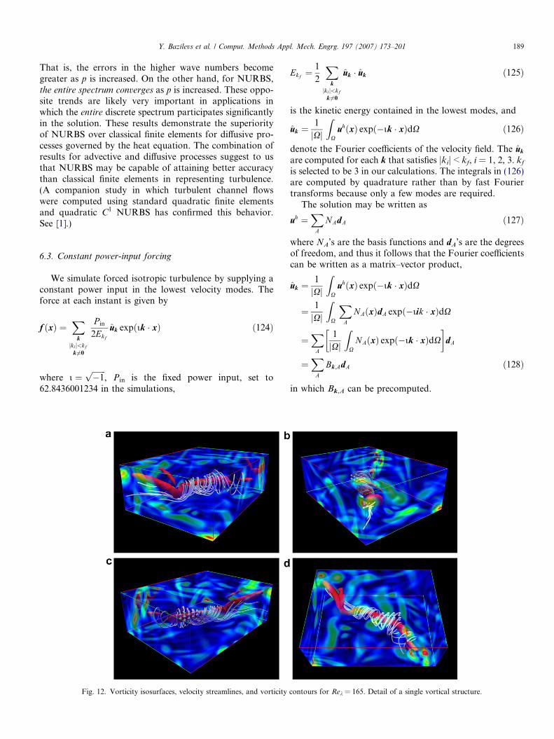
6.3. Constant power-input forcing
We simulate forced isotropic turbulence by supplying aconstant power input in the lowest velocity modes. Theforce at each instant is given by
f ðxÞ ¼X
kjki j<kf
k6¼0
P in
2Ekf
uk expðik � xÞ ð124Þ
where i ¼ffiffiffiffiffiffiffi�1p
, Pin is the fixed power input, set to62.8436001234 in the simulations,
Fig. 12. Vorticity isosurfaces, velocity streamlines, and vorticity
Ekf ¼1
2
Xk
jkij<kfk 6¼0
uk � uk ð125Þ
is the kinetic energy contained in the lowest modes, and
uk ¼1
jXj
ZX
uhðxÞ expð�ik � xÞdX ð126Þ
denote the Fourier coefficients of the velocity field. The uk
are computed for each k that satisfies jkij < kf, i = 1, 2, 3. kf
is selected to be 3 in our calculations. The integrals in (126)are computed by quadrature rather than by fast Fouriertransforms because only a few modes are required.
The solution may be written as
uh ¼X
A
NAdA ð127Þ
where NA’s are the basis functions and dA’s are the degreesof freedom, and thus it follows that the Fourier coefficientscan be written as a matrix–vector product,
uk ¼1
jXj
ZX
uhðxÞ expð�ik � xÞdX
¼ 1
jXj
ZX
XA
NAðxÞdA expð�iik � xÞdX
¼X
A
1
jXj
ZX
NAðxÞ expð�ik � xÞdX
�dA
¼X
A
Bk;AdA ð128Þ
in which Bk,A can be precomputed.
contours for Rek = 165. Detail of a single vortical structure.

190 Y. Bazilevs et al. / Comput. Methods Appl. Mech. Engrg. 197 (2007) 173–201
6.4. Test cases
We consider two cases, Rek = 165 and Rek =1, whereRek is the Taylor microscale Reynolds number [58].
For Rek = 165 the kinematic viscosity, m, is set to 1/150.The kinetic energy is computed as
256
0.01
0.1
1
10
1 10
64
32
128
0.01
0.1
1
10
1 10
32
64128
0.01
0.1
1
10
1 10
32
64
Fig. 13. Energy spectra for h-refinement. Rek =1.
q2 ¼ 1
2jXj
ZX
uhðxÞ � uhðxÞdX ð129Þ
which fluctuates about 41, ±15%, in all cases. Thus,
Rek ¼2q2
3
ffiffiffiffiffi15
�m
rð130Þ
256
1
10
10 100
128
64
32
64
10 100 1
1032
128
32
100 1
10
64
10
Fig. 14. Two-point third-order structure functions for h-refinement.Rek =1.

Y. Bazilevs et al. / Comput. Methods Appl. Mech. Engrg. 197 (2007) 173–201 191
is about 165 for all cases, where � is the dissipation (see[58]). Once the simulation reaches equilibrium, the powerinput, Pin, is equal to the dissipation of the simulation. Thisresult is in good agreement with the DNS data. Results arecompared with the data provided by Moser, which is de-scribed in [52]. For Rek =1 the viscosity is set to zero.In this case we compare with theoretical correlations (see[58]).
0.01
0.1
1
10
1 10
P=1
P=3
P=2
0.01
0.1
1
10
1 10
P=3
P=2
P=1
0.01
0.1
1
10
1 10
P=1
P=2
Fig. 15. Energy spectra for k-refinement. Rek =1.
6.5. Simulation results
The quantities of interest are the energy spectrum andthe two-point third-order structure function. The two-point third-order structure function is defined as
S3ðrÞ ¼ hðuðxþ rÞ � uðxÞÞ3i; ð131Þ
10 1
10
P=2
P=3
P=1
100
100 1
10
P=1
P=2
P=3
10
100 1
10
P=2
P=1
10
Fig. 16. Two-point third-order structure functions for k-refinement.Rek =1.

192 Y. Bazilevs et al. / Comput. Methods Appl. Mech. Engrg. 197 (2007) 173–201
where hÆi implies ensemble average. In the inertial sub-range, S3 scales like r for fully-developed, locally isotropicturbulence (see [58, p. 204]). Due to the role played by S3 inthe Karman–Howarth equation, an accurate representa-tion of S3 implies an accurate description of the energytransfer in the inertial subrange.
Data samples were collected for at least 20 eddy turn-over times, Tett = q2/(2�). Samples were separated by about0.4 Tett. The spatial sampling is performed at knots and themid-points between knots. For example, in the simulationof 323, we sample on a 643 uniform mesh.
Remarks
(1) We investigated the possibility that q1, the parame-ter in the generalized-a method that controls itsnumerical high-frequency dissipation, affected results.
Fig. 17. Illustration of the wall-normal discretization for the turbulent channelto better resolve boundary layers. Note that, due to the open knot vectorinterpolatory at the endpoints of the domain, which facilitates strong imposit
We ran cases with q1 = 1 (no dissipation), 0.5 (ourdefault value) and 0 (maximal dissipation). We foundno discernible differences in the computed statistics.This may have been due to the very small time stepsused in the calculations, typically of the order of 0.2the advective Courant number, where the advectivespeed is defined as
ffiffiffiqp
.(2) We note that it is important to precisely converge the
nonlinear residual of the coarse-scale equations in everytime step. We reduced the residual in each step to 10�5
of its initial value. Failure to sufficiently converge theresidual leads to spurious dissipation in our experience.
The data are presented in two complementary fashions.Figs. 6, 7, 13, and 14 illustrate h-refinement, whereasFigs. 8, 9, 15 and 16 illustrate k-refinement (see [30]).
flow problem. Meshes are graded towards the ends of the interval in orderconstruction (see [30] for details), the first and last basis functions are
ion of no-slip Dirichlet boundary conditions.

Y. Bazilevs et al. / Comput. Methods Appl. Mech. Engrg. 197 (2007) 173–201 193
6.5.1. Rek = 165
Fig. 6 shows that the energy spectrum has no energy pileup at high-wave numbers for all orders and numbers ofdegrees-of-freedom. In fact, all energy spectra are in goodagreement with the DNS, even for coarse meshes. InFig. 6, we observe that about half the wave numbers forlinear basis functions are in close agreement with theDNS spectrum, while this ratio significantly improves forhigher-order basis functions, becoming almost 100% forthe cubic case at 643. In Fig. 7, the third-order structurefunction is plotted against the non-dimensional distance
Linear
0
5
10
15
20
25
0.1 1 0
5
10
15
20
25
0.1 1
32
64
0.5
1
1.5
0
0.5
1
1.5
0.5
1
1.5
2
2.5
3
3.5
4
0 100 2
0.5
1
1.5
0
0.5
1
1.5
0.5
1
1.5
2
2.5
3
3.5
4
0 100 2
DNS 32
32
DNS
Fig. 18. Turbulent channel flow at Res = 395 computed usin
r/g, where g is the Kolmogorov dissipative scale [58],defined as
g ¼ m3
�
� �1=4
: ð132Þ
As r/g increases the velocity field should decorrelate, whichis observed in our calculations and the DNS. However, theforcing utilized in the DNS is somewhat different than thatutilized here. In the DNS, the forcing occurs within a sphereof radius 3 in spectral space, whereas in our calculations, the
DNS
10 100 10 100
64
Linear
00 300 40000 300 400
64
g linear NURBS: h-refinement interpretation of results.

194 Y. Bazilevs et al. / Comput. Methods Appl. Mech. Engrg. 197 (2007) 173–201
forcing was performed within a box of half-edge-length 3.Thus, the small discrepancies between our results and theDNS for large values of r/g are to be expected. Fig. 7 showsthat for each order, improved agreement with DNS is at-tained by increasing the number of degrees-of-freedom.Figs. 8 and 9 show that order elevation improves the agree-ment with DNS. It is particularly evident from these figures,that the most significant payoff is achieved when increasingthe order from linear to quadratic.
Figs. 10 and 11 show snapshots of vorticity isosurfacesand velocity streamlines computed on a 1283 mesh of
Quadratic
0
5
10
15
20
25
0.1 1 0
5
10
15
20
25
0.1 1
32
32
0.5
1
1.5
0
0.5
1
1.5
0.5
1
1.5
2
2.5
3
3.5
4
0 100 2
0.5
1
1.5
0
0.5
1
1.5
0.5
1
1.5
2
2.5
3
3.5
4
0 100 2
DNS 32
DNS
64
Fig. 19. Turbulent channel flow at Res = 395 computed using
quadratic NURBS. Fig. 12 shows a detail of a single vortextube computed on a mesh of 643 cubic NURBS. The visu-alizations are performed using techniques from Johnsonet al. [46,47].
6.5.2. Rek =1The Rek =1 case (i.e., m = 0) is felt to be relevant to
practical engineering situations in which the resolution isinadequate to represent the physical flow features, evenwith an LES approach (see [54]). What one hopes to seein an LES is a distinct branch of the energy spectrum
DNS
10 100 10 100
64
Quadratic
00 300 40000 300 400
64
quadratic NURBS: h-refinement interpretation of results.

Y. Bazilevs et al. / Comput. Methods Appl. Mech. Engrg. 197 (2007) 173–201 195
corresponding to the inertial range, without an energy pile-up at the cut-off wave number. Likewise, there is a theoret-ical inertial-range scaling for the two-point third-orderstructure function. In the present circumstances, the forc-ing occurs for jkij < kf = 3, i = 1,2,3, but beyond this valuewe expect to see a transition to an inertial range, at least fora sufficiently fine mesh.
From Figs. 13 and 15, we observe that, for all ordersand discretizations, no energy pile up occurs in the highestwave numbers in the computed energy spectra. Beyond theregime of forcing, the expected Kolmogorov k�5/3 spec-trum is clearly discernible. It is interesting to observe fromFig. 13 that the tail off of the spectrum at high wave num-
Cubic
64
0
5
10
15
20
25
0.1 1 0
5
10
15
20
25
0.1 1
0.5
1
1.5
0
0.5
1
1.5
0.5
1
1.5
2
2.5
3
3.5
4
0 100 2
0.5
1
1.5
0
0.5
1
1.5
0.5
1
1.5
2
2.5
3
3.5
4
0 100 2
DNS 32
DNS
32
64
Fig. 20. Turbulent channel flow at Res = 395 computed usin
bers diminishes as the order of approximation is increased.To facilitate the comparison of Figs. 14 and 16 with Figs. 7and 9, respectively, we employ the same scaling in Figs. 14and 16 as the one we used in Figs. 7 and 9. In Figs. 14 and16 we emphasize this point by the notation g165. Again, thedevelopment of the inertial range is evident.
7. Turbulent channel flow
Our next numerical example is an equilibrium turbulentchannel flow at Reynolds number 395 based on the frictionvelocity and the channel half width. The computationaldomain is a rectangular box of size 2p · 2 · 2/3p in the
10 100 10 100
32
DNS
Cubic
00 300 40000 300 400
64
g cubic NURBS: h-refinement interpretation of results.
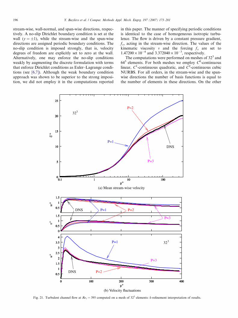
196 Y. Bazilevs et al. / Comput. Methods Appl. Mech. Engrg. 197 (2007) 173–201
stream-wise, wall-normal, and span-wise directions, respec-tively. A no-slip Dirichlet boundary condition is set at thewall (y = ±1), while the stream-wise and the span-wisedirections are assigned periodic boundary conditions. Theno-slip condition is imposed strongly, that is, velocitydegrees of freedom are explicitly set to zero at the wall.Alternatively, one may enforce the no-slip conditionsweakly by augmenting the discrete formulation with termsthat enforce Dirichlet conditions as Euler–Lagrange condi-tions (see [6,7]). Although the weak boundary conditionapproach was shown to be superior to the strong imposi-tion, we did not employ it in the computations reported
332
0
5
10
15
20
25
0.1 1 0
5
10
15
20
25
0.1 1 0
5
10
15
20
25
0.1 1
P=1
0.5
1
1.5
0
0.5
1
1.5
0.5
1
1.5
2
2.5
3
3.5
4
0 100 2
0.5
1
1.5
0
0.5
1
1.5
0.5
1
1.5
2
2.5
3
3.5
4
0 100 2
0.5
1
1.5
0
0.5
1
1.5
0.5
1
1.5
2
2.5
3
3.5
4
0 100 2
P=1
DNS P=2
DNS P=1
Fig. 21. Turbulent channel flow at Res = 395 computed on a m
in this paper. The manner of specifying periodic conditionsis identical to the case of homogeneous isotropic turbu-lence. The flow is driven by a constant pressure gradient,fx, acting in the stream-wise direction. The values of thekinematic viscosity m and the forcing fx are set to1.47200 · 10�4 and 3.372040 · 10�3, respectively.
The computations were performed on meshes of 323 and643 elements. For both meshes we employ C0-continuouslinear, C1-continuous quadratic, and C2-continuous cubicNURBS. For all orders, in the stream-wise and the span-wise directions the number of basis functions is equal tothe number of elements in these directions. On the other
DNS
10 100 10 100 10 100
P=3
P=2
332
00 300 40000 300 40000 300 400
P=3
P=3
P=2
esh of 323 elements: k-refinement interpretation of results.
Y. Bazilevs et al. / Comput. Methods Appl. Mech. Engrg. 197 (2007) 173–201 197
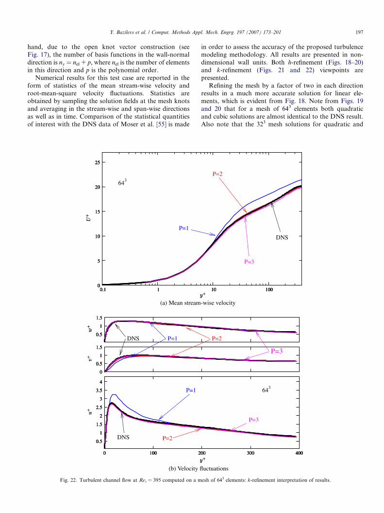
hand, due to the open knot vector construction (seeFig. 17), the number of basis functions in the wall-normaldirection is ny = nel + p, where nel is the number of elementsin this direction and p is the polynomial order.
Numerical results for this test case are reported in theform of statistics of the mean stream-wise velocity androot-mean-square velocity fluctuations. Statistics areobtained by sampling the solution fields at the mesh knotsand averaging in the stream-wise and span-wise directionsas well as in time. Comparison of the statistical quantitiesof interest with the DNS data of Moser et al. [55] is made
643
0
5
10
15
20
25
0.1 1 0
5
10
15
20
25
0.1 1 0
5
10
15
20
25
0.1 1
P=1
0.5
1
1.5
0
0.5
1
1.5
0.5
1
1.5
2
2.5
3
3.5
4
0 100 2
0.5
1
1.5
0
0.5
1
1.5
0.5
1
1.5
2
2.5
3
3.5
4
0 100 2
0.5
1
1.5
0
0.5
1
1.5
0.5
1
1.5
2
2.5
3
3.5
4
0 100 2
P=1
DNS P=2
DNS P=1
Fig. 22. Turbulent channel flow at Res = 395 computed on a m
in order to assess the accuracy of the proposed turbulencemodeling methodology. All results are presented in non-dimensional wall units. Both h-refinement (Figs. 18–20)and k-refinement (Figs. 21 and 22) viewpoints arepresented.
Refining the mesh by a factor of two in each directionresults in a much more accurate solution for linear ele-ments, which is evident from Fig. 18. Note from Figs. 19and 20 that for a mesh of 643 elements both quadraticand cubic solutions are almost identical to the DNS result.Also note that the 323 mesh solutions for quadratic and
DNS
10 100 10 100 10 100
P=3
P=2
364
00 300 40000 300 40000 300 400
P=3
P=3
P=2
esh of 643 elements: k-refinement interpretation of results.

198 Y. Bazilevs et al. / Comput. Methods Appl. Mech. Engrg. 197 (2007) 173–201
cubic NURBS are significantly more accurate than the 643
mesh solution for linear elements (compare Figs. 19 and 20with 18).
In Fig. 21, on the 323 mesh, linear elements show a sig-nificant over-prediction of the mean stream-wise velocity inthe log layer. Fluctuations in the stream-wise velocity arealso over-predicted as compared to the DNS result. Onthe same mesh, quadratic and cubic NURBS show goodaccuracy in both mean and fluctuating quantities. Noticethe significant increase in accuracy when going from linearto quadratic NURBS, while increasing the order ofapproximation to cubic yields results that are not much dif-ferent than for quadratic NURBS. The same trends are evi-dent in Fig. 22. However, here it is clear that the quadraticand cubic results are virtually identical to the DNS results.
The results for 323 quadratic and cubic NURBS areeven better than high-fidelity spectral Galerkin LES resultspresented in [36,27]. We note though that the formulationutilized in [36,27] employed a fine-scale eddy viscositymodel and is quite different from the one used here.
Fig. 23 shows isosurfaces of stream-wise velocity, veloc-ity streamlines, and a series of snapshots of particlesreleased at the channel inflow and set in motion to followthe streamlines in the boundary layer.
Fig. 23. Turbulent channel flow at Res = 395. Flow streamlines and isosurfacesgreen, are released at the channel inflow close to the wall (see (a)), and are set inas particles travel down the length of the channel (see (b)–(d)). One can see thetravel at slower speeds compared to the ones released in the outer layer. Also noas they approach the outflow, revealing the presence of faster and slower streaksused for this visualization.
8. Conclusions
We presented a general variational multiscale theorysuitable for LES-type turbulence modeling. The theory isderived directly from the incompressible Navier–Stokesequations and does not involve any ad hoc mechanisms.In particular, it entirely avoids use of eddy viscosities.We feel that this theory of turbulence modeling is morefundamental and logically consistent than ones derivedheretofore and it has significant potential in practical engi-neering calculations. One of the primary reasons we feelthis way is that NURBS, in the context of the isogeometricconcept [30,19,5]), are capable of precisely modeling com-plex geometric configurations. This feature was notexploited herein where we focused on the physics of turbu-lence in simple geometries, but the code we utilized is thesame one we have successfully employed in a variety ofcomplex laminar and turbulent, fluid and fluid–structureinteraction computations (see [3,4,77]). We might also men-tion that the turbulence modeling aspects remain unaltered
when we consider laminar flows. In this sense, our method-ology may be viewed as an approach for solving the incom-pressible Navier–Stokes equations, whether the flow underconsideration is laminar or turbulent, or both (see [14]). We
of stream-wise velocity. Two parallel planes of particles, colored white andmotion to follow the streamlines. Snapshots of the particle field are shownformation of the boundary layer as the particles released closer to the wallte that the particles initially released on different planes are mixed togetherin the boundary layer. Solution on the mesh of 323 quadratic NURBS was

Y. Bazilevs et al. / Comput. Methods Appl. Mech. Engrg. 197 (2007) 173–201 199
also believe that this aspect separates our theory of turbu-lence modeling from predecessors.
The calculations we performed of forced homogeneousisotropic turbulence and turbulent channel flows demon-strated that even the simplest residual-based modeling offine scales by asymptotic scaling arguments is capable ofgiving very good results, at least in the LES context. Nev-ertheless, we feel that this is an area in which it is almostinevitable that there will be significant improvement.Research is under way to develop better approximationsto fine-scale behavior. We may mention the importantwork of Codina et al. [16] and work that we also have inprogress and hope to report on in the near future.
We wish to emphasize the importance of the fine-scalemodeling problem. It represents the only open issue withinour theory of turbulence modeling because the coarse-scaleequation, the one we solve numerically, is exact in the sensethat the dependence on the fine scales is exact, that is, there isno approximation until the fine scales are substituted into it.For this reason, we feel significant effort should be devotedto studying the fine-scale problem, both theoretically andcomputationally. One area that deserves attention is directlyaddressing nonlinearities in the fine-scale approximationrather than dealing with them through perturbation and lin-earization procedures. In the context of scaling arguments,an initial investigation was performed in [14].
The role of NURBS should also not be underestimated,at least in comparison with classical finite elements. Weshowed through dispersion analysis of one-dimensionalmodel problems that NURBS gave significantly betterapproximations of advective and diffusive behavior. Thiswas particularly dramatic in the high-wave number portionof the spectrum in diffusive processes. We conjectured thatthis was an advantage in LES turbulence modeling due tothe participation of all resolved wave numbers in a numer-ical calculation. In a companion study we performed acomparison of NURBS and classical finite elements on tur-bulent channel flows, and the results confirmed our conjec-ture (see [1]).
The gold standard in turbulence has always been spec-tral methodology. NURBS give near-spectral approxima-tions yet are applicable to the most complex geometriesthrough the isogeometric concept. Although classical finiteelements are capable of approximating complex geome-tries, they are not capable of high-precision geometricmodeling because curved geometries are modeled withpiece-wise polynomial facets. On the other hand, NURBSare undoubtedly the most widely used technology for mod-eling curved surfaces in geometric design, and even qua-dratic NURBS are capable of exactly representing allconic sections (i.e., circles, cylinders, spheres, ellipsoids,etc.), which are ubiquitous in engineering design. Further-more, it is not yet fully appreciated how poorly classicalhigher-order finite elements approximate higher wave num-bers. We believe the divergent behavior of the approxima-tion with increasing order is a deficiency in turbulence, and,we conjecture, in other situations as well. On the contrary,
the good behavior of NURBS over the entire wave-numberspectrum, combined with their superiority in geometricrepresentation, seem to make them an ideal general pur-pose technology for turbulent flow simulation of complexengineering designs.
An issue that needs to be investigated is the relationship,if any, with compact finite differences (see [53]). If a rela-tionship can be established, it may be very beneficial in gen-eralizing compact finite differences to complex geometriesand in suggesting fast computer implementations ofNURBS approximations.
Given that the scale separation in the present methodol-ogy is performed with respect to the coarse-scale spaceactually used in the numerical computations, that is, theresolved scales, and that the fine-scale approximation isrendered well defined by a projector used to make precisethe direct sum decomposition into coarse and fine scales,it is impossible to entirely separate modeling and numericalconcepts. We accept this as a fact associated with correctLES-type modeling concepts, not a shortcoming. However,other modeling concepts are certainly possible within thevariational multiscale framework, including ones, whichare not directly associated with numerical approximation,such as is the case of RANS.
We also believe that our theory is more coherent math-ematically than previous formulations and that it may bepossible to use it as a basis of a statistical analysis of con-vergence and approximation. This would represent a verysignificant step forward for the theory of turbulence mod-eling, but, admittedly, a very difficult one to achieve. Nev-ertheless, we feel a door has been opened for theconstruction of a mathematical theory.
We found quadratic NURBS to give very significant accu-racy advantages over linear elements. This, combined withtheir geometric approximation superiority, and small com-putational overhead compared with linear elements (about50% in our computations), suggests to us that they shouldbe considered a preferred practical tool for engineering com-putations. Cubics, on the other hand, increased cost consid-erably (by about 100% compared to quadratics), largely dueto cache overflow in element calculations. These remarksneed to be qualified by the fact that our implementation ofhigher-order elements is not yet optimized in any way. Wehope to significantly improve efficiency in future work.
In summary, we feel a new paradigm for turbulencemodeling has been established. Initial results seem to indi-cate its accuracy per degree of freedom is superior or, at theleast, equal to any procedure proposed heretofore. Its gen-erality and geometric flexibility also suggest it may providea more powerful approach to turbulence calculations thanpreviously existed.
Acknowledgements
We wish to express our appreciation for support pro-vided by the Office of Naval Research under ContractNo. N00014-03-0263, Dr. Luise Couchman, contract
200 Y. Bazilevs et al. / Comput. Methods Appl. Mech. Engrg. 197 (2007) 173–201
monitor, and Sandia National Laboratories under ContractNo. 114166. We also wish to thank R.D. Moser for guid-ance and many helpful suggestions, his students, AmitabhBhattacharya and Paolo Zandonade, for their help withthe isotropic turbulence DNS data, Greg Johnson andKarla Vega of Texas Advanced Computing Center [71]for the visualizations in Figs. 10–12 and 23. We also wouldlike to thank TACC for granting us access to their comput-ing facilities. Y. Bazilevs was partially supported by the J.T.Oden ICES Postdoctoral Fellowship at the Institute forComputational Engineering and Sciences (ICES). A. Realiwas partially supported by the J.T. Oden Faculty Fellow-ship Research Program at the ICES. G. Scovazzi waspartially supported under Sandia Laboratories LDRD‘‘A Mathematical Framework for Multiscale Scienceand Engineering: The Variational Multiscale Methodand Interscale Transfer Operators’’, contract monitorDr. S. Scott Collis. This support is gratefully acknowledged.
References
[1] I. Akkerman, Y. Bazilevs, V.M. Calo, T.J.R. Hughes, S. Hulshoff,The role of continuity in residual-based variational multiscalemodeling of turbulence. Comput. Mech., 2007, doi: doi:10.1007/s00466-007-0193-7.
[2] G.I. Barenblatt, Similarity, Self-similarity, and Intermediate Asympt-otics, Cambridge University Press, 1996.
[3] Y. Bazilevs. Isogeometric Analysis of Turbulence and Fluid–Struc-ture Interaction, PhD Thesis, ICES, UT Austin, 2006.
[4] Y. Bazilevs, V.M. Calo, Y. Zhang, T.J.R. Hughes, Isogeometricfluid–structure interaction analysis with applications to arterial bloodflow, Comput. Mech. 38 (2006) 310–322.
[5] Y. Bazilevs, L. Beirao da Veiga, J.A. Cottrell, T.J.R. Hughes, G.Sangalli, Isogeometric analysis: approximation, stability and errorestimates for h-refined meshes, Math. Mod. Methods Appl. Sci. 16(2006) 1031–1090.
[6] Y. Bazilevs, T.J.R. Hughes, Weak imposition of Dirichlet boundaryconditions in fluid mechanics, Comp. Fluids 36 (2007) 12–26.
[7] Y. Bazilevs, C. Michler, V.M. Calo, T.J.R. Hughes, Weak Dirichletboundary conditions for wall-bounded turbulent flows, Comp.Methods Appl. Mech. Engrg., in press, 2007, doi:10.1016/j.cma.2007.06.026.
[8] M. Behr, D. Hastreiter, S. Mittal, T.E. Tezduyar, Incompressible flowpast a circular cylinder: dependence of the computed flow field on thelocation of the lateral boundaries, Comp. Methods Appl. Mech.Engrg. 123 (1996) 309–316.
[9] P.B. Bochev, T.J.R. Hughes, G. Scovazzi, A Multiscale Discontin-uous Galerkin Method, Springer Lecture Notes in Computer Science,vol. 3743, Springer, 2006.
[10] F. Brezzi, L.P. Franca, T.J.R. Hughes, A. Russo, b ¼R
g, Comp.Methods Appl. Mech. Engrg. 145 (1997) 329–339.
[11] L. Brillouin, Wave Propagation in Periodic Structures, DoverPublications Inc., 1953.
[12] A.N. Brooks, T.J.R. Hughes, Streamline upwind/Petrov–Galerkinformulations for convection dominated flows with particular empha-sis on the incompressible Navier–Stokes equations, Comp. MethodsAppl. Mech. Engrg. 32 (1982) 199–259.
[13] A. Buffa, T.J.R. Hughes, G. Sangalli, Analysis of the multiscalediscontinuous Galerkin method for convection–diffusion problems,SIAM J. Numer. Anal. 44 (4) (2006) 1420–1440.
[14] V.M. Calo, Residual-based Multiscale Turbulence Modeling: FiniteVolume Simulation of Bypass Transition, PhD Thesis, Department ofCivil and Environmental Engineering, Stanford University, 2004.
[15] J. Chung, G.M. Hulbert, A time integration algorithm for structuraldynamics with improved numerical dissipation: The generalized-amethod, J. Appl. Mech. 60 (1993) 371–375.
[16] R. Codina, J. Principe, O. Guasch, S. Badia, Time dependentsubscales in the stabilized finite element approximation of incom-pressible flow problems, Comp. Methods Appl. Mech. Engrg. 196(2007) 2413–2430.
[17] E. Cohen, R. Riesenfeld, G. Elber, Geometric Modeling with Splines.An Introduction, A.K. Peters Ltd., Wellesley, MA, 2001.
[18] S.S. Collis, Multiscale Methods for Turbulence Simulation andControl, Technical Report 034, MEMS, Rice University, 2002.
[19] J.A. Cottrell, A. Reali, Y. Bazilevs, T.J.R. Hughes, Isogeometricanalysis of structural vibrations, Comp. Methods Appl. Mech. Engrg.195 (2006) 5257–5297.
[20] C. Farhat, B. Koobus. Finite volume discretization on unstructuredmeshes of the multiscale formulation of large eddy simulations, in: F.G.Rammerstorfer, H.A. Mang, J. Eberhardsteiner (Eds.), Proceedings ofthe Fifth World Congress on Computational Mechanics (WCCM V),Vienna University of Technology, Austria, July 7–12, 2002.
[21] G.E. Farin, NURBS Curves and Surfaces: From Projective Geometryto Practical Use. A.K. Peters, Ltd., Natick, MA, 1995.
[22] V. Gravemeier, The variational multiscale method for laminar andturbulent flow, Arch. Comput. Methods Engrg. – State of the ArtRev. 13 (2006) 249–324.
[23] P.M. Gresho, R.L. Sani, Incompressible Flow and the Finite ElementMethod, Wiley, New York, NY, 1998.
[24] G. Hauke, M.H. Doweidar, M. Miana, The multiscale approach toerror estimation and adaptivity, Comp. Methods Appl. Mech. Engrg.195 (2006) 1573–1593.
[25] G. Hauke, M.H. Doweidar, M. Miana, Proper intrinsic scales for a-posteriori multiscale error estimation, Comp. Methods Appl. Mech.Engrg. 195 (2006) 3983–4001.
[26] J. Hoffman, C. Johnson, Stability of the dual Navier–Stokesequations and efficient computation of mean output in turbulentflow using adaptive DNS/LES, Comp. Methods Appl. Mech. Engrg.195 (2006) 1709–1721.
[27] J. Holmen, T.J.R. Hughes, A.A. Oberai, G.N. Wells, Sensitivity ofthe scale partition for variational multiscale LES of channel flow,Phys. Fluids 16 (3) (2004) 824–827.
[28] T.J.R. Hughes, Multiscale phenomena: Green’s functions, theDirichlet-to-Neumann formulation, subgrid scale models, bubblesand the origins of stabilized methods, Comp. Methods Appl. Mech.Engrg. 127 (1995) 387–401.
[29] T.J.R. Hughes, The Finite Element Method: Linear Static andDynamic Finite Element Analysis, Dover Publications, Mineola, NY,2000.
[30] T.J.R. Hughes, J.A. Cottrell, Y. Bazilevs, Isogeometric analysis:CAD, finite elements, NURBS, exact geometry, and mesh refinement,Comp. Methods Appl. Mech. Engrg. 194 (2005) 4135–4195.
[31] T.J.R. Hughes, G. Feijoo, L. Mazzei, J.B. Quincy, The variationalmultiscale method–Aparadigm for computational mechanics, Comp.Methods Appl. Mech. Engrg. 166 (1998) 3–24.
[32] T.J.R. Hughes, M. Mallet, A new finite element formulation for fluiddynamics: III. The generalized streamline operator for multidimen-sional advective–diffusive systems, Comp. Methods Appl. Mech.Engrg. 58 (1986) 305–328.
[33] T.J.R. Hughes, L. Mazzei, K.E. Jansen, Large-eddy simulation andthe variational multiscale method, Comp. Vis. Sci. 3 (2000) 47–59.
[34] T.J.R. Hughes, L. Mazzei, A.A. Oberai, A.A. Wray, The multiscaleformulation of large eddy simulation: decay of homogenous isotropicturbulence, Phys. Fluids 13 (2) (2001) 505–512.
[35] T.J.R. Hughes, A.A. Oberai, Calculation of shear stresses in Fourier–Galerkin formulations of turbulent channel flows: projection, theDirichlet filter and conservation, J. Comput. Phys. 188 (1) (2003) 281–295.
[36] T.J.R. Hughes, A.A. Oberai, L. Mazzei, Large-eddy simulation ofturbulent channel flows by the variational multiscale method, Phys.Fluids 13 (6) (2001) 1784–1799.

Y. Bazilevs et al. / Comput. Methods Appl. Mech. Engrg. 197 (2007) 173–201 201
[37] T.J.R. Hughes, G. Sangalli, Variational multiscale analysis: the fine-scale Green’s function, projection, optimization, localization, andstabilized methods, SIAM J. Numer. Anal. 45 (2007) 539–557.
[38] T.J.R. Hughes, G. Scovazzi, P.B. Bochev, A. Buffa, A multiscalediscontinuous Galerkin method with the computational structure of acontinuous Galerkin method, Comp. Methods Appl. Mech. Engrg.195 (2006) 2761–2787.
[39] T.J.R. Hughes, G. Scovazzi, L.P. Franca, Multiscale and stabilizedmethods, in: E. Stein, R. De Borst, T.J.R. Hughes (Eds.), Encyclo-pedia of computational mechanics, Computational Fluid Dynamics,vol. 3, Wiley, 2004 (Chapter 4).
[40] T.J.R. Hughes, J. Stewart, A space-time formulation for multiscalephenomena, J. Comput. Appl. Math. 74 (1996) 217–229.
[41] T.J.R. Hughes, G.N. Wells, A.A. Wray, Energy transfers and spectraleddy viscosity of homogeneous isotropic turbulence: comparison ofdynamic Smagorinsky and multiscale models over a range ofdiscretizations, Phys. Fluids 16 (2004) 4044–4052.
[42] K.E. Jansen, S.S. Collis, C.H. Whiting, F. Shakib, A betterconsistency for low-order stabilized finite element methods, Comp.Methods Appl. Mech. Engrg. 174 (1999) 153–170.
[43] K.E. Jansen, C.H. Whiting, G.M. Hulbert, A generalized-a methodfor integrating the filtered Navier–Stokes equations with a stabilizedfinite element method, Comp. Methods Appl. Mech. Engrg. 190(1999) 305–319.
[44] H. Jeanmart, G.S. Winckelmans. Comparison of recent dynamicsubgrid-scale models in the case of the turbulent channel flow, in:Proceedings of the Summer Program, Center for TurbulenceResearch, Stanford University and NASA Ames, 2002.
[45] C. Johnson, Numerical Solution of Partial Differential Equations bythe Finite Element Method, Cambridge University Press, Sweden,1987.
[46] G.P. Johnson, V.M. Calo, K. Gaither. Interactive visualization andanalysis of transitional flow, IEEE Trans. Vis. Comp. Graphics,submitted for publication.
[47] G.P. Johnson, K. Gaither, V.M. Calo. Visualizing turbulent flow, in:15th IEEE Visualization Conference, Austin, TX, October 2004, p.598.22.
[48] B. Koobus, C. Farhat, A variational multiscale method for the largeeddy simulation of compressible turbulent flows on unstructuredmeshes – application to vortex shedding, Comp. Methods Appl.Mech. Engrg. 193 (2004) 1367–1383.
[49] A.G. Kravchenko, P. Moin, R. Moser, Zonal embedded grids fornumerical simulation of wall-bounded turbulent flows, J. Comput.Phys. 127 (1996) 412–423.
[50] A.G. Kravchenko, P. Moin, K. Shariff, B-spline method and zonalgrids for simulation of complex turbulent flows, J. Comput. Phys. 151(1999) 757–789.
[51] W.Y. Kwok, R.D. Moser, J. Jimenez, A critical evaluation of theresolution properties of B-spline and compact finite differencemethods, J. Comput. Phys. 174 (2001) 510–551.
[52] J.A. Langford, R.D. Moser, Optimal LES formulations for isotropicturbulence, J. Fluid Mech. 398 (1999) 321–346.
[53] S.K. Lele, Compact finite difference schemes with spectral-likeresolution, J. Comput. Phys. 103 (1992) 16–42.
[54] M. Lesieur, O. Metais, P. Comte, Large Eddy Simulation ofTurbulence, Cambridge University Press, Cambridge, England, 2005.
[55] R. Moser, J. Kim, R. Mansour, DNS of turbulent channel flow up toRe = 590, Phys. Fluids 11 (1999) 943–945.
[56] A.A. Oberai, T.J.R. Hughes, The variational multiscale formulationof LES: channel flow at Res = 590, in: 40th AIAA Ann. Mtg., Reno,NV, 2002, AIAA 2002-1056.
[57] L. Piegl, W. Tiller, The NURBS Book (Monographs in VisualCommunication), 2nd ed., Springer-Verlag, New York, 1997.
[58] S.B. Pope, Turbulent Flows, Cambridge University Press, Cam-bridge, 2000.
[59] S. Ramakrishnan, S.S. Collis, Variational multiscale modeling forturbulence control, in: AIAA 1st Flow Control Conference, St. Louis,MO, June 2002, AIAA 2002-3280.
[60] S. Ramakrishnan and S.S. Collis. Multiscale modeling for turbulencesimulation in complex geometries, in: 40th AIAA Aerospace SciencesMeeting and Exhibit, Reno, NV, Jan. 2004, AIAA 2004-0241.
[61] S. Ramakrishnan, S.S. Collis, Turbulence control simulation usingthe variational multiscale method, AIAA J. 42 (4) (2004) 745–753.
[62] S. Ramakrishnan, S.S. Collis, Partition selection in multiscaleturbulence modeling, Phys. Fluids 18 (7) (2006).
[63] D.F. Rogers, An Introduction to NURBS with Historical Perspec-tive, Academic Press, San Diego, CA, 2001.
[64] Y. Saad, M.H. Schultz, GMRES: a generalized minimal residualalgorithm for solving nonsymmetric linear systems, SIAM J. Sci. Stat.Comput. 7 (1986) 856–869.
[65] P. Sagaut, S. Deck, M. Terracol, Multiscale and MultiresolutionApproaches in Turbulence, Imperial College Press, 2006.
[66] G. Scovazzi. Multiscale Methods in Science and Engineering, PhDThesis, Department of Mechanical Engineering, Stanford University.http://www.cs.sandia.gov/ gscovaz, 2004.
[67] F. Shakib, T.J.R. Hughes, Z. Johan, A new finite element formulationfor computational fluid dynamics: X. The compressible Euler andNavier–Stokes equations, Comp. Methods Appl. Mech. Engrg. 89(1991) 141–219.
[68] K. Shariff, R.D. Moser, Two-dimensional mesh embedding for B-spline methods, J. Comput. Phys. 145 (1998) 471–488.
[69] V. Sheffer, An inviscid flow with compact support in space-time, J.Geom. Anal. 3 (1993) 343–401.
[70] J.C. Simo, T.J.R. Hughes, Computational Inelasticity, Springer-Verlag, New York, 1998.
[71] Texas Advanced Computing Center (TACC). http://www.tacc.utexas.edu.
[72] T.E. Tezduyar, Computation of moving boundaries and interfacesand stabilization parameters, Int. J. Numer. Methods Fluids 43(2003) 555–575.
[73] R. Vichnevetsky, J.B. Bowles, Fourier Analysis of NumericalApproximations of Hyperbolic Equations, Society for Industrialand Applied Mathematics, Philadelphia, 1982.
[74] G.B. Whitham, Linear and Nonlinear Waves, John Wiley and Sons,New York, 1974.
[75] C.H. Whiting, Stabilized Finite Element Methods for Fluid Dynamicsusing a Hierarchical Basis, PhD Thesis, Rensselaer PolytechnicInstitute, September 1999.
[76] C.H. Whiting, K.E. Jansen, A stabilized finite element method for theincompressible Navier–Stokes equations using a hierarchical basis,Int. J. Numer. Methods Fluids 35 (2001) 93–116.
[77] Y. Zhang, Y. Bazilevs, S. Goswami, C. Bajaj, T.J.R. Hughes, Patient-specific vascular NURBS modeling for isogeometric analysis of bloodflow, Comp. Methods Appl. Mech. Engrg. 196 (2007) 2943–2959.