a visual velocity impedance controller
TRANSCRIPT

University of New MexicoUNM Digital Repository
Mechanical Engineering ETDs Engineering ETDs
Fall 12-17-2016
A Visual Velocity Impedance ControllerVictor Nevarez
Follow this and additional works at: https://digitalrepository.unm.edu/me_etds
Part of the Mechanical Engineering Commons
This Thesis is brought to you for free and open access by the Engineering ETDs at UNM Digital Repository. It has been accepted for inclusion inMechanical Engineering ETDs by an authorized administrator of UNM Digital Repository. For more information, please contact [email protected].
Recommended CitationNevarez, Victor. "A Visual Velocity Impedance Controller." (2016). https://digitalrepository.unm.edu/me_etds/112

i

A Visual Velocity Impedance Controller
by
Victor Nevarez
Bachelors of Science, Mechanical Engineering,
Massachusetts Institute of Technology, 2012
THESIS
Submitted in Partial Fulfillment of the
Requirements for the Degree of
Master of Science
Mechanical Engineering
The University of New Mexico
Albuquerque, New Mexico
December, 2016

iii
Dedication
This work is dedicated to my parents and to Johanna Chong. Without them I doubt
I would have ever come this far or pushed myself as much as I have. As much as I
have struggled they have always been there to help me out and helped me push
through.

iv
Acknowledgments
I would like the thank everyone who helped in contributing the writing of this thesis.First of all, Dr. Ron Lumia for advising me through all these years and providingme with the invaluable research experiences over the years. More than any classesI have taken at UNM, the research experience and valuable lessons that ProfessorLumia has given me are the most important things I have taken from the graduateprogram. I would like to thank my committee members, Dr. Rafael Fierro and Dr.Joseph Bishop, for everything they have taught me and for taking time to reviewthis work.
I would like to thank Dave Vick for showing me how to use the various robots inthe High Bay Area. I would also like to thank Tim Blada for showing me how to usethe WAM’s and for getting me started on making my own controller for the WAM.Without the work provided by time I would not have been able to finish this workat all.
Finally, I would like to thank my mom, dad, sister, and Johanna for all theirsupport. Without them keeping me accountable I fear to think how much longer thiswork would have taken to finish.

v
A Visual Velocity Impedance Controller
by
Victor Nevarez
Bachelors of Science, Mechanical Engineering,
Massachusetts Institute of Technology, 2012
M.S., Mechanical Engineering, University of New Mexico, 2016
Abstract
Successful object insertion systems allow the object to translate and rotate to ac-
commodate contact forces. Compliant controllers are used in robotics to provide this
accommodation. The impedance compliant controller is one of the more researched
and well known compliant controllers used for assembly. The velocity filtered visual
impedance controller is introduced as a compliant controller to improve upon the
impedance controller. The velocity filtered impedance controller introduces a filter
of the velocity impedance and a gain from the stiffness. The velocity impedance
controller was found to be more stable over larger ranges of stiffness values than
the position based impedance controller. This led to the velocity impedance con-
troller being more accurate and stable with respect to external forces. The velocity
impedance controller was also found to have a better compliant response when tested
on various insertion geometries in various configurations, including a key insertion
acting against gravity. Finally, a novel kinetic friction cone compliance model is
introduced for the velocity impedance controller. It was determined that the new
compliance model provided a more reliable insertion than the standard insertion
model by increasing the error tolerance for failure.

vi
Contents
List of Figures x
1 Introduction 1
1.1 Problem . . . . . . . . . . . . . . . . . . . . . . . . . . . . . . . . . . 1
1.2 Contribution . . . . . . . . . . . . . . . . . . . . . . . . . . . . . . . . 3
1.3 Impact . . . . . . . . . . . . . . . . . . . . . . . . . . . . . . . . . . . 3
1.4 Scope of Work . . . . . . . . . . . . . . . . . . . . . . . . . . . . . . . 5
1.5 Thesis outline . . . . . . . . . . . . . . . . . . . . . . . . . . . . . . . 5
2 Literature Review 7
2.1 Literature Review . . . . . . . . . . . . . . . . . . . . . . . . . . . . . 7
2.1.1 Assembly . . . . . . . . . . . . . . . . . . . . . . . . . . . . . 8
2.1.2 Compliant Motion: Impedance Control . . . . . . . . . . . . . 9
2.1.3 Visual Servoing: Visual Impedance Control . . . . . . . . . . . 11
2.1.4 Friction Cones . . . . . . . . . . . . . . . . . . . . . . . . . . . 13
2.2 Summary . . . . . . . . . . . . . . . . . . . . . . . . . . . . . . . . . 16

Contents vii
3 Hardware and Testing 17
3.1 Hardware . . . . . . . . . . . . . . . . . . . . . . . . . . . . . . . . . 17
4 Object Insertion 21
4.1 Peg and Hole Model . . . . . . . . . . . . . . . . . . . . . . . . . . . 21
4.2 Insertion Geometry Analysis . . . . . . . . . . . . . . . . . . . . . . . 38
4.3 Key Insertion Modeling . . . . . . . . . . . . . . . . . . . . . . . . . . 43
5 Visual Position Impedance Controller 46
5.1 Impedance Controller Modeling . . . . . . . . . . . . . . . . . . . . . 47
5.2 Vision Modeling . . . . . . . . . . . . . . . . . . . . . . . . . . . . . . 50
5.3 Controller Simulation of Single Joint . . . . . . . . . . . . . . . . . . 54
5.4 Controller Response . . . . . . . . . . . . . . . . . . . . . . . . . . . . 59
5.4.1 Non-Contact motion . . . . . . . . . . . . . . . . . . . . . . . 60
5.4.2 External Force Response . . . . . . . . . . . . . . . . . . . . . 62
5.4.3 Vision Control Response . . . . . . . . . . . . . . . . . . . . . 64
5.5 Insertion Testing . . . . . . . . . . . . . . . . . . . . . . . . . . . . . 65
5.5.1 Circular Peg Insertions . . . . . . . . . . . . . . . . . . . . . . 67
5.5.2 Square Peg Insertion . . . . . . . . . . . . . . . . . . . . . . . 70
5.5.3 Cross Peg Insertion . . . . . . . . . . . . . . . . . . . . . . . . 72
5.5.4 Cross Insertion against Gravity . . . . . . . . . . . . . . . . . 73
5.5.5 Key Insertion . . . . . . . . . . . . . . . . . . . . . . . . . . . 77

Contents viii
5.6 Summary . . . . . . . . . . . . . . . . . . . . . . . . . . . . . . . . . 80
6 Velocity Filtered Impedance Controller 81
6.1 Velocity Filter Impedance Model and Simulation . . . . . . . . . . . . 81
6.1.1 Simulation Results . . . . . . . . . . . . . . . . . . . . . . . . 85
6.2 Controller Response . . . . . . . . . . . . . . . . . . . . . . . . . . . . 89
6.2.1 Non-Contact Motion . . . . . . . . . . . . . . . . . . . . . . . 90
6.2.2 External Force Response . . . . . . . . . . . . . . . . . . . . . 94
6.2.3 Visual Control Response . . . . . . . . . . . . . . . . . . . . . 96
6.3 Insertions Testing . . . . . . . . . . . . . . . . . . . . . . . . . . . . . 99
6.3.1 Circular Peg . . . . . . . . . . . . . . . . . . . . . . . . . . . . 99
6.3.2 Square Peg . . . . . . . . . . . . . . . . . . . . . . . . . . . . 101
6.3.3 Cross Peg . . . . . . . . . . . . . . . . . . . . . . . . . . . . . 104
6.3.4 Against Gravity Peg . . . . . . . . . . . . . . . . . . . . . . . 106
6.3.5 Key Insertion . . . . . . . . . . . . . . . . . . . . . . . . . . . 109
7 Velocity Impedance Controller with Kinetic Friction Cone 112
7.1 Kinetic Friction Cone Insertion Model . . . . . . . . . . . . . . . . . 112
7.1.1 Kinetic Friction Wedging Model . . . . . . . . . . . . . . . . . 115
7.1.2 Kinetic Friction Jamming Model . . . . . . . . . . . . . . . . 117
7.1.3 Kinetic Friction Cone Compliance Model . . . . . . . . . . . . 118
7.2 Insertion Testing with Kinetic Friction Cone Model . . . . . . . . . . 121

Contents ix
7.2.1 Cross Insertion . . . . . . . . . . . . . . . . . . . . . . . . . . 123
7.2.2 Cross Insertion Against Gravity . . . . . . . . . . . . . . . . . 127
7.2.3 Key Insertion . . . . . . . . . . . . . . . . . . . . . . . . . . . 129
7.3 Summary . . . . . . . . . . . . . . . . . . . . . . . . . . . . . . . . . 132
8 Conclusion 134
References 136

x
List of Figures
1.1 Basic Control Scheme. . . . . . . . . . . . . . . . . . . . . . . . . . 2
1.2 Basic Control Scheme [61]. Where R is the force vector, N is the
vertical force contribution, and T is the horizontal contribution. φ is
the friction cone angle and µ is the coefficient of static friction. . . . 4
2.1 Modes of Failure Jamming (A) and Wedging (B) . . . . . . . . . . . 14
2.2 Key inserted in lock [23] . . . . . . . . . . . . . . . . . . . . . . . . . 15
3.1 Experiment setup. . . . . . . . . . . . . . . . . . . . . . . . . . . . 18
3.2 Experiment setup. Insertion of circular peg into fixed block. . . . . . 19
4.1 Chamferless insertion . . . . . . . . . . . . . . . . . . . . . . . . . . 22
4.2 Chamfered insertion . . . . . . . . . . . . . . . . . . . . . . . . . . . 23
4.3 Modes of Failure Jamming (A) and Wedging (B) . . . . . . . . . . . 24
4.4 Diagram of chamferless peg partially inserted. . . . . . . . . . . . . 26
4.5 Wedging failure . . . . . . . . . . . . . . . . . . . . . . . . . . . . . 27
4.6 Friction cones during wedging . . . . . . . . . . . . . . . . . . . . . 28

List of Figures xi
4.7 lateral error . . . . . . . . . . . . . . . . . . . . . . . . . . . . . . . 29
4.8 Wedging model diagram . . . . . . . . . . . . . . . . . . . . . . . . . 31
4.9 Jamming Diagram . . . . . . . . . . . . . . . . . . . . . . . . . . . . 32
4.10 Force model for one point contact stage. . . . . . . . . . . . . . . . . 33
4.11 Force model for two point contact stage. . . . . . . . . . . . . . . . . 36
4.12 Cross sections of multiple geometries . . . . . . . . . . . . . . . . . . 38
4.13 Change in wedging diagram . . . . . . . . . . . . . . . . . . . . . . . 41
4.14 Cross section of key hole model . . . . . . . . . . . . . . . . . . . . . 44
5.1 Impedance Controller . . . . . . . . . . . . . . . . . . . . . . . . . . 49
5.2 Controller model . . . . . . . . . . . . . . . . . . . . . . . . . . . . . 51
5.3 Vision controller integrated with the impedance controller . . . . . . 52
5.4 Camera coordinate system . . . . . . . . . . . . . . . . . . . . . . . 53
5.5 Peg detection . . . . . . . . . . . . . . . . . . . . . . . . . . . . . . . 54
5.6 Ellipse highlighting detected peg. . . . . . . . . . . . . . . . . . . . . 55
5.7 Position impedance simulation model . . . . . . . . . . . . . . . . . 55
5.8 Position impedance simulation model with external environment . . 56
5.9 Impedance simulation response without external environment . . . . 58
5.10 Impedance simulation model with external environment . . . . . . . 58
5.11 Unstable impedance controller response . . . . . . . . . . . . . . . . 59
5.12 Position response of impedance controller . . . . . . . . . . . . . . . 60

List of Figures xii
5.13 Pose response of both controllers . . . . . . . . . . . . . . . . . . . . 61
5.14 Both responses against gravity . . . . . . . . . . . . . . . . . . . . . 62
5.15 Position controller contact force . . . . . . . . . . . . . . . . . . . . 63
5.16 Position controller unstable contact force . . . . . . . . . . . . . . . 64
5.17 Position visual controller . . . . . . . . . . . . . . . . . . . . . . . . 65
5.18 Peg testing dimensions . . . . . . . . . . . . . . . . . . . . . . . . . 66
5.19 Circular peg insertion errors . . . . . . . . . . . . . . . . . . . . . . 67
5.20 Circular jamming response . . . . . . . . . . . . . . . . . . . . . . . 68
5.21 Circular insertion force response . . . . . . . . . . . . . . . . . . . . 69
5.22 Square peg insertion errors . . . . . . . . . . . . . . . . . . . . . . . 70
5.23 Square jamming response . . . . . . . . . . . . . . . . . . . . . . . . 71
5.24 Square insertion force response . . . . . . . . . . . . . . . . . . . . . 72
5.25 Cross peg insertion errors . . . . . . . . . . . . . . . . . . . . . . . . 73
5.26 Cross jamming response . . . . . . . . . . . . . . . . . . . . . . . . . 74
5.27 Square insertion force response . . . . . . . . . . . . . . . . . . . . . 74
5.28 Cross peg insertion against gravity errors . . . . . . . . . . . . . . . 75
5.29 Cross jamming against gravity response . . . . . . . . . . . . . . . . 76
5.30 Cross insertion force against gravity response . . . . . . . . . . . . . 76
5.31 WAM holding key to be inserted into keyhole . . . . . . . . . . . . . 77
5.32 Key insertion errors . . . . . . . . . . . . . . . . . . . . . . . . . . . 78
5.33 Key jamming . . . . . . . . . . . . . . . . . . . . . . . . . . . . . . . 79

List of Figures xiii
5.34 Key insertion force . . . . . . . . . . . . . . . . . . . . . . . . . . . . 79
6.1 Velocity impedance simulation model . . . . . . . . . . . . . . . . . 82
6.2 Velocity impedance simulation model with external environment . . 83
6.3 Velocity impedance simulation response without external environment 85
6.4 Both impedance simulation response without external environment . 86
6.5 Velocity impedance simulation response with external environment . 87
6.6 Both impedance simulation response with external environment . . . 87
6.7 Velocity impedance controller response to high stiffness environment 88
6.8 Both impedance controller response to high stiffness environment . . 89
6.9 Velocity controller pose response . . . . . . . . . . . . . . . . . . . . 90
6.10 Velocity controller response of position in direction of gravity . . . . 91
6.11 Velocity controller pose acting against gravity . . . . . . . . . . . . . 91
6.12 Comparison of position response between the velocity impedance con-
troller and the position based impedance controller . . . . . . . . . . 92
6.13 Comparison of pose response between the velocity impedance con-
troller and the position based impedance controller . . . . . . . . . . 93
6.14 Velocity impedance position response at high stiffness . . . . . . . . 93
6.15 Velocity impedance pose response at high stiffness . . . . . . . . . . 94
6.16 Velocity controller contact force . . . . . . . . . . . . . . . . . . . . 95
6.17 Force response comparison . . . . . . . . . . . . . . . . . . . . . . . 96
6.18 Velocity controller with high and low stiffness values . . . . . . . . . 97

List of Figures xiv
6.19 Velocity visual controller . . . . . . . . . . . . . . . . . . . . . . . . 97
6.20 Comparison of visual controllers . . . . . . . . . . . . . . . . . . . . 98
6.21 Circle peg insertion wedging . . . . . . . . . . . . . . . . . . . . . . 99
6.22 Circle peg insertion jamming . . . . . . . . . . . . . . . . . . . . . . 100
6.23 Circle peg insertion force . . . . . . . . . . . . . . . . . . . . . . . . 101
6.24 Square peg insertion wedging . . . . . . . . . . . . . . . . . . . . . . 102
6.25 Square peg insertion jamming . . . . . . . . . . . . . . . . . . . . . 103
6.26 Square peg insertion force . . . . . . . . . . . . . . . . . . . . . . . . 103
6.27 Cross peg insertion wedging . . . . . . . . . . . . . . . . . . . . . . . 104
6.28 Cross peg insertion jamming . . . . . . . . . . . . . . . . . . . . . . 105
6.29 Cross peg insertion force . . . . . . . . . . . . . . . . . . . . . . . . 105
6.30 Cross peg against gravity insertion wedging . . . . . . . . . . . . . . 107
6.31 Cross peg against gravity insertion jamming . . . . . . . . . . . . . 108
6.32 Cross peg against gravity insertion force . . . . . . . . . . . . . . . . 108
6.33 Key insertion wedging . . . . . . . . . . . . . . . . . . . . . . . . . . 109
6.34 Key insertion jamming . . . . . . . . . . . . . . . . . . . . . . . . . 110
6.35 Key insertion force . . . . . . . . . . . . . . . . . . . . . . . . . . . . 111
7.1 Kinetic Friction Model . . . . . . . . . . . . . . . . . . . . . . . . . 113
7.2 Wedging comparison between KFC model and Whitney model . . . 116
7.3 Jamming comparison between KFC model and Whitney model . . . 117

List of Figures xv
7.4 Minimum Kinetic friction stiffness profile . . . . . . . . . . . . . . . 119
7.5 Kinetic stiffness profile . . . . . . . . . . . . . . . . . . . . . . . . . 120
7.6 Model of kinetic friction cone controller. (KFC-VIC) . . . . . . . . . 122
7.7 Cross peg Whitney and KFC model comparison for KFC-VIC . . . . 123
7.8 Cross peg Whitney and KFC model comparison for VIC . . . . . . . 124
7.9 Cross peg insertion jamming . . . . . . . . . . . . . . . . . . . . . . 125
7.10 Cross peg insertion force . . . . . . . . . . . . . . . . . . . . . . . . 126
7.11 Comparison for Whitney and KFC model for insertion against gravity
for the KFC-VIC . . . . . . . . . . . . . . . . . . . . . . . . . . . . 127
7.12 Comparison for Whitney and KFC model for insertion against gravity
for the VIC . . . . . . . . . . . . . . . . . . . . . . . . . . . . . . . . 128
7.13 Cross peg insertion force against gravity . . . . . . . . . . . . . . . . 129
7.14 Comparison for Whitney and KFC model for key insertion for the
KFC-VIC . . . . . . . . . . . . . . . . . . . . . . . . . . . . . . . . . 130
7.15 Comparison for Whitney and KFC model for key insertion for the VIC131
7.16 Key insertion force . . . . . . . . . . . . . . . . . . . . . . . . . . . . 132

1
Chapter 1
Introduction
This chapter presents the velocity based visual impedance controller and introduces
the object insertion problem to test the controller. The problem overview and the
controller setup will be discussed in this chapter. This chapter also establishes how
the rest of the thesis will be organized.
1.1 Problem
Compliant motion control is an important robotic technique for manufacturing. In
particular, compliant motion control is useful when a robot must interact with a rigid
environment, another robot, or a human. Object insertion is a great application to
test a compliant motion controller. Compliant motion is needed because orientation
errors can cause jamming or wedging during insertion.
This thesis will use a difficult key and hole insertion to demonstrate the capa-
bilities of a new type of compliant motion controller. The proposed controller is
a velocity filtered visual impedance controller. The key and hole insertion is used
because of the precise position and orientation required.

Chapter 1. Introduction 2
Impedance
Controller Robot Target Object
Manipulator feedback
IBVS
Task
Velocity Control
Vision System
Figure 1.1: Basic Control Scheme.
The velocity filtered impedance controller will use image based visual servoing
(IBVS) combined with an impedance controller. Figure 1.1 depicts the relationship
between the IBVS and the impedance controller. With this velocity filtered visual
impedance controller, a robot will insert a key and generate a friction cone during the
insertion controlling the velocity of the manipulator. Friction cones are the space in
which an applied force will not slip. The cone determines the maximum angle before
slipping occurs. In robotics the friction cone is used as a configuration space model.
This thesis will use a dynamic friction cone approach instead of this static friction
cone. After modeling a kinetic friction cone for an insertion problem, a robot can
learn the most effective path to travel and adjust its forces for a successful motion.
The hypothesis is that by using a velocity filtered visual impedance controller a
robot is capable of extremely difficult object insertions such as key insertion. By
using a velocity based approach the robot will be able to generate a kinetic friction
cone for an improved object insertion compared to the position based position based

Chapter 1. Introduction 3
impedance control.
1.2 Contribution
This thesis develops a reliable vision filtered impedance controller by using a fusion
of an impedance controller and an image based visual servoing (IBVS) controller
while introducing the new velocity filter to the controller. Using this velocity filtered
impedance controller, this thesis will develop a method to build the novel kinetic
friction compliance model for challenging insertions used in mechanical assembly.
This thesis will also demonstrate the improvement in object insertions when using
a velocity filtered impedance controller compared to the position based impedance
controller.
1.3 Impact
Using a velocity based approach will improve upon the impedance controller by
increasing the range of stability to higher stiffness values. This is important for object
insertion since the positional and pose accuracy will ensure a successful insertion.
As will be shown later, higher stiffness values will lead to more accurate motions
and will also increase the insertion force needed for object insertion. This velocity
based approach also ensures stability in the high stiffness environment that would
be encountered during more difficult insertions such as the key insertion. As will
also be shown, the position impedance controller can start to lose stability in these
confined environments due to the friction forces. Using a velocity filtered impedance
controller for difficult insertions, such as the key insertion, will not only show that
it is a viable and more stable control method but will also show the practicality of a
kinetic friction cone model.

Chapter 1. Introduction 4
Figure 1.2: Basic Control Scheme [61]. Where R is the force vector, N is the verticalforce contribution, and T is the horizontal contribution. φ is the friction cone angleand µ is the coefficient of static friction.
With the capabilities from the velocity impedance controller, it is possible to
create a kinetic friction cone compliance model. A kinetic friction cone shares the
same principles as the static friction cone, shown in Figure 1.2; however, with the
kinetic friction cone we want the force vector to be outside of the friction cone. To
do this the insertion force will need to be adjusted accordingly, as will be shown
later. Using the kinetic friction cone compliance model and controlling the velocity
to navigate through the insertion, it is possible to wiggle the object to the goal
position.
Ultimately, this controller and kinetic fiction cone compliance model can be ap-
plied to a number of real problems including welding, grinding, dragging an object,
and of course, object insertion.

Chapter 1. Introduction 5
1.4 Scope of Work
The focus of the thesis is to introduce a novel impedance controller. The work in this
thesis is to expand upon well known position based methods for control and showcase
a velocity based analog for the proposed controller. This thesis will also introduce
a kinetic friction cone compliance model, modeled after the static friction cone, to
prevent insertion failure. For the vision controller this work uses an IBVS controller
to improve the impedance controller’s accuracy. Using these velocity analogs in
comparison with the position based methods this thesis will showcase the benefits of
using a velocity based impedance controller.
1.5 Thesis outline
Chapter 2 presents the current state of the art in object insertion and impedance
control. Chapter 3 describes the hardware used for the experiments. Chapter 4
defines the object insertion model as well as compares the difficulty of insertion for
various geometries with respect to jamming and wedging, the two types of failure
for object insertion. Chapter 5 defines the impedance controller, first modeling the
controller and modeling the vision control. Next the chapter will demonstrate the
simulation implementation of the model using Simulink, and then the results from
the robot. At the end of chapter 5 the insertion results for the position impedance
controller will be discussed. Chapter 6 defines the velocity impedance controller,
again modeling the controller, showing simulation results, and then results from the
robot. Chapter 6 results will compare the position impedance controller’s responses
from chapter 5 to the results from the velocity impedance controller. The end of
chapter 6 will have insertion results from the velocity impedance controller and will
compare these results with the insertions from the position impedance controller.
Chapter 7 defines and models the kinetic friction cone model. In this chapter the

Chapter 1. Introduction 6
compliance model will be defined and the velocity impedance controller stiffness
will be optimized with respect to the accuracy of the robot. At the end of this
chapter the compliance model will be tested against various insertions and compared
to the previous insertion results from the velocity impedance controller. Chapter
8 concludes the thesis with a review of the research and the potential benefits for
future work.

7
Chapter 2
Literature Review
The past twenty years has had a large push in robotics research to allow robots to
replace humans in various dangerous tasks. These tasks range from bomb disposal
to detecting environments with hostile threats. The issue is that these types of tasks
are difficult to accomplish since the robot needs to be as capable as a human that
would perform them. In these tasks a robot is likely to have to open a door. One of
the most difficult but useful object insertions for a robot is a key insertion.
2.1 Literature Review
An important field of research previously discussed is the manipulation of unknown
objects. Some of the most common objects that robots will encounter are doors.
Most of the dangerous tasks in which robots would replace humans require mobility
in human-made environments. To navigate through a room, a robot will have to
recognize a door and interact with it to open it [26]. To open the door, the robot
needs to apply a delicate amount of force and also has to be capable of compensating
for various changes in the environment that it cannot detect such as a stiff door hinge.

Chapter 2. Literature Review 8
For a robot to accomplish a task with fine motion, it needs to be capable of
compliant motion. Compliant motion controllers can interact with objects passively
or actively. Active compliance interacts with objects by controlling the external
forces applied on the robot or using visual feedback.
2.1.1 Assembly
In the past ten years robotics in assembly has been focused on improving upon tasks
currently completed by humans. The two main reasons to replace humans with
robots is because of either the danger involved with the task, i.e., handling radioactive
material, or improves upon the efficiency and time to complete a task. There has
been interest in determining the most efficient use of multi-robotic production for the
automotive industry [27]. There has also been work done in crowd sourcing swarm
manipulation methods to determine how to improve cooperative manipulation in
work spaces [3]. There has also been an increased focus in manipulation of small
objects, as these tasks often prove difficult for humans [56].
Although many of these tasks can be accomplished by robots, there is still a
significant difference in the accuracy and repeatability that humans can achieve.
This is mostly due to the compliance humans provide when they interact with their
environments. To address this there have been an interest in research in robotic
assisted assembly. Some of these experiments include using robotic limbs to lift
and assemble heavy objects through these supernumerary robotic limbs [40]. In one
work, the human worker uses robotic limbs to assist in aircraft fuselage assembly
[39]. There has even been interest in robots cooperating with humans to complete
assembly tasks as well [12].
Although there is considerable research in cooperative robotic and human assem-
bly, there is still a reluctance to introduce humans in robotic work spaces. This is
due to most industrial robotic controllers being position based controllers. These

Chapter 2. Literature Review 9
types of controllers move straight to the task and adjust their position based on the
error from the goal. Without compliance, the robot will collide with objects that
may be in the path the robot is traveling. With compliance, the robot can soften
the collision and become safer to use alongside humans.
2.1.2 Compliant Motion: Impedance Control
Compliant motion can be categorized in two ways: active or passive [25] [49]. Passive
compliance does not require the robot to know how it is interacting with the envi-
ronment but instead allows the hardware to naturally interact with objects. This
can be a desirable compliant motion if the environment and objects are well-known.
For object insertion, error corrective compliance is used since the contact forces al-
ways push the object towards the insertion goal [42]. Passive compliance may be the
technique humans use to insert objects [15].
The issue with passive compliance is the limitations of its compliance, i.e., com-
pliance in only a single dimension. As such, passive compliance is not typically used
to interact with objects. Instead, active compliance is typically used in robotic sys-
tems. Active compliance differs in that it needs a sensor to detect the interaction
with the environment to help control the motion. One of the few ways to achieve
active compliance is to use a hybrid of force and position control [45]. Compliant
motion is not limited to active or passive, there are hybrid types of compliant mo-
tions that are also used [51]. Typically these hybrid motions are decomposed into the
active parts and the passive parts of the motion. These hybrid compliant controllers
have even been used to grasp various objects [54].
Another technique is to use haptic controllers, which commonly rely on config-
uration spaces to provide force feedback [13, 31, 46, 11]. Haptic control relies on
modeling the forces that the robot experiences; through this interaction the robot
can perceive the forces. As such configuration spaces need to be created to limit

Chapter 2. Literature Review 10
the forces and directions in which the robot can interact in the environment. The
friction cone is a configuration space representation of the overall stiffness of the
environment when interacting with an object in various directions [31]. Another im-
portant compliance method that relies on modeling the stiffness of the environment
is an impedance controller.
Impedance control is a concept popularized by Neville Hogan in 1985 [14]. The
general idea was to treat the manipulator of the robot as an object that has impedance,
in other words treat the manipulator as something with variable stiffness and damp-
ing. By changing the apparent stiffness and damping of the manipulator, it is possible
to execute compliant moves. More formally, the impedance of the system is repre-
sented as a transfer function of the system that can either be a ratio of displacement
over input force or of velocity to input force.
This type of controller uses the position, velocity, and output force of the manip-
ulator. Using these multiple inputs, the robot is capable of interacting with external
forces applied by the environment. Since the impedance is capable of interacting
with external forces, it is capable of gross and fine motion [14]. The difficult task in
using impedance controllers is determining the impedance for each task. There have
been methods in how to use force references to improve the impedance controller [47],
methods that use impedance controllers without torque feedback [21], and methods
in varying the impedance depending on the environment [17].
There have been stiffness based tuning methods to improve the adaptability of
robot-assisted rehabilitation [24], as well as non-linear adaptive impedance controllers
also intended for rehabilitation purposes [36]. There have even been fuzzy adaptation
impedance controllers used for peg in hole insertions [2]. The impedance controller
has even been used with predictive controllers intended to prevent mechanical losses,
i.e., losses from friction and external forces [10]. In terms of assembly based methods,
there are impedance controllers that provide high-speed position and force responses
for compliant microgrippers [57].

Chapter 2. Literature Review 11
Various types of impedance control system uses different sensory feedback [44].
In particular, there are impedance controllers that use a vision system to maintain
the desired contact with the robot and the object [32]. These visual impedance
controllers typically estimate the position and the pose of the robot and object and
provide a hybrid visual/force controller [22]. There are various other types of visual
controllers that can be coupled with an impedance controller.
Velocity based impedance methods have been tested and found to be useful and
stable [41, 8, 5]. Using a velocity based method insures that the steady state error
will be zero. This type of impedance controller has been found to be stable in high
stiffness environments using high damping values. This thesis will differ from these
methods in that the velocity impedance contribution will filter the impedance force
and the stiffness of the robot will act as a gain. Based on the stability models used
from the position based impedance model [37] and also through impedance methods
that have used integrator control [20] we have found that this method will also be
able to improve upon the stability due to the stiffness being significantly larger than
the damping.
2.1.3 Visual Servoing: Visual Impedance Control
Visual servoing consists of using information of the environment extracted by one or
several cameras to control the movements of a robot [4]. This allows for a wide range
of tasks that can be achieved such as object tracking, object manipulation, visual
guided motion, and even object insertion [50]. Image based visual servoing is a field
of research where control is based on feature points in the image plane [7]. This is a
robust visual control method since the robot can account for disturbance and noise.
IBVS can track the motion trajectories of objects in an image to execute tasks that
other vision based controllers cannot accomplish due to image based errors [9].
The major disadvantage of visual control is that these camera internal parameters

Chapter 2. Literature Review 12
must be known through calibration. There is also the issue of depth. Since most
environments are unknown, the typically 2D-sensor is not capable of extracting depth
without some type of reference. Camera calibrations are broken into two categories:
intrinsic calibration and extrinsic calibration. Intrinsic calibration determines the
internal parameters of each camera, such as focal length and pixel height/width.
Extrinsic parameters are the parameters that relate the objects in the environment,
depth and rotation, back to the camera. This includes the transformation matrix
from camera to the origin and the depths of feature points in the image.
Intrinsic camera calibration methods have been thoroughly researched and un-
derstood [60, 59, 52]. Typically calibration objects are well defined object, already
known geometries. Camera calibration is done by taking multiple images of these cal-
ibration objects and determines the intrinsic parameters of each camera from these
images. Extrinsic camera calibration is a bit more difficult since determining the
environment’s depth requires some sort of reference. The use of reference points or
fiduciaries can simplify extrinsic calibration since these reference points are known
and provide enough information in the image to determine the extrinsic parameters
[16]. Extrinsic camera calibration in an unknown environment is much more difficult
since known reference points cannot be used. There are methods that achieve this
calibration by moving unknown detected objects in the environment and taking as
many images as needed until the parameters are determined [58]. The issue with
this type of method is that it tends to be costly computationally.
There are calibration methods that are capable of extracting both the intrinsic
and extrinsic parameters online. In other words, it is possible to do calibration in
unknown environments by navigating in the environment and simultaneously cali-
brating the vision system [1]. One particular method of online calibration is to use
circular motions around a feature point to extract all calibration parameters [34].
Once a camera is fully calibrated to its environment, it is possible to accurately con-
trol the robot using any visual servoing technique. As mentioned before, there exist

Chapter 2. Literature Review 13
visual/force hybrid controllers, which allow the robot to detect and interact with
various object in the environment [43].
Visual impedance controllers use the visual data and provide feedback from the
environment to an impedance controller [33]. A visual impedance controller uses
vision to determine position and orientation errors. Figure 1.1, shows the basic
control scheme for a visual impedance controller. In this case the velocity is provided
by vision instead of position. An example of a vision based impedance approach is
to follow the contours of an object’s edge [18]. By using an impedance controller, a
robot performing edge tracking can smooth out the trajectories and can accomplish
these motions at high velocities without sacrificing accuracy. Although there are
velocity based impedance controllers, there are no velocity based visual impedance
controllers.
Visual impedance controllers have also been used for the task of object insertion
[53] [48]. These controllers are very useful for insertion because of the orientation
required to properly insert an object. To prevent failure the initial orientation of the
object must be within a certain tolerance. It is difficult to determine whether the
object is within this tolerance without vision. Using these vision control methods
the robot is capable of fixing the orientation errors in real time and improving the
chances of a successful insertion.
2.1.4 Friction Cones
Object insertion is the one of the best methods to test a compliant controller. Object
insertion has been shown to depend on how the objects interact with each other as
they pass through different contact states [55]. The two types of failure during the
insertion are known as jamming and wedging, shown in Figure 2.1. Wedging occurs
when a contact force becomes compressive and holds the object in place. To avoid
wedging, the orientation error of the object insertion must always be minimized.

Chapter 2. Literature Review 14
Inser�on ForceInser�on Force
Compressive
contact forcesCompressive
contact forces
(A) (B)
Figure 2.1: Modes of Failure Jamming (A) and Wedging (B)
Jamming occurs when the insertion force is misaligned with the insertion axis. To
avoid this failure, the object needs to rotate to compensate for the misalignment[55].
One particular method to avoid both types of failures is to create friction cones.
A friction cone is a 3 dimensional representation of the friction angle. The friction
angle is determined as the maximum angle a force vector can have before slipping
occurs [35]. This is shown in Figure 1.2. The friction cone was found to be bounded
by the following relationship,
tan(θ) = µ, (2.1)
where θ is the friction angle defined by the force vector and µ is the coefficient of
friction.
Friction cones in robotics are ranges created in configuration space that determine

Chapter 2. Literature Review 15
whether an insertion will be successful as long as the robot avoids entering this space
[6]. By creating these regions, it is possible to know which motions will succeed with
insertion and which will fail [38]. The concept of the friction cone is not limited to
insertion. It has also been applied in grasping objects [30].
Figure 2.2: Key inserted in lock [23]
The friction cone is not limited to modeling the static friction limits; it can also be
applied to Coulombic friction [29]. For this thesis we will introduce a kinetic friction
cone that will model the kinetic friction the same way the friction cone models the
static friction limits.
Key insertion is an extremely difficult object insertion task due to the geometric
constraints. A door that may need to be opened by a robot may be locked, so the
robot needs to be capable to insert a key and rotate it to unlock the door. Here
lies the major problem; not only must the object be fully inserted, must be able to
rotate after insertion. Figure 2.2 shows how the key must be aligned before being
able rotate it to unlock it. There is similar work in rotating inserted objects into

Chapter 2. Literature Review 16
object with varying friction[19]. This work is important since the robot needs to be
able to distinguish between when it is capable of rotating and when it is not.
2.2 Summary
Robotic assembly continues to grow as a field and will accelerate with the use of
compliant controllers. The impedance controller was originally introduced when the
hardware did not exist to realize the controller [14]. Now that the hardware exists, the
impedance controller has been used to complete various assembly tasks. To improve
upon the accuracy of the impedance control system the impedance controller has
been used in various vision control systems. With the recent developments in visual
servoing, the accuracy and capabilities of the impedance controller has improved and
grown. Finally, through the use of configuration space models such as friction cones,
the impedance controller has improved its compliance capabilities, which can be very
useful for object insertion. The position based position impedance controller tends
to go unstable in high stiffness environments normally encountered during insertion.
The need to improve the stability of the impedance controller at high stiffness still
exists.

17
Chapter 3
Hardware and Testing
The system developed and tested in this thesis consists of equipment from the
Robotics Lab in UNM’s South Campus MTTC building. The system consists of a
Barrett Technology Whole Arm Manipulator (WAM), two cameras, reflective mem-
ory, a computer controller, and stationary objects for insertion. An example of the
experimental setup for the key insertion is shown in Figure 3.1 .
3.1 Hardware
The WAM is a 7 degree-of-freedom robotic arm developed by Barrett Technology.
The WAM communicates through reflective memory to a target computer, which
controls the robot through a Simulink controller. For this thesis, a velocity based
impedance controller was implemented in Simulink, compiled, and loaded onto a
xpctarget through Matlab. For the xpctarget to communicate with the WAM the
xpctarget communicates directly to the reflective memory using C/C++ wrappers.
The xpctarget communicates with the reflective memory by reading and writing from
specific memory addresses, called nodes. The WAM has an on-board computer that
also reads and writes to the reflective memory. Specifically, the controller computer

Chapter 3. Hardware and Testing 18
Camera
Key
Door
WAM
Controller Computer
Reflec�ve Memory
Camera
On Board Computer
Figure 3.1: Experiment setup.
writes 6 stiffness, 6 damping, 7 joint torques, and 6 goal positions while the WAM’s
on board computer writes the 7 current joint torques and the 7 current joint angles
of the WAM. The controller computer reads the goal positions, the current joint
angles, and the current joint torque while the WAM’s on board computer reads the
stiffness, damping, motor currents, force, and joint torques.
The controller computer, the computer running the Simulink controller, has a 2.4
GHz Intel processor and eight Gigabytes of RAM. The controller computer simul-
taneously reads the WAM’s position, calculates the next position in the trajectory,
and also communicates with the vision systems to determine how to adjust the tra-
jectory. For the vision systems, a Logitech c270 and c260 cameras were used. Both
cameras have resolution up to 1280 × 720 and communicate via USB. To commu-
nicate to Matlab, additional drivers had to be installed using a webcam toolbox for
image processing. The image processing done in Matlab sends the results to the
impedance controller in Simulink , which sends the positional and compliance data

Chapter 3. Hardware and Testing 19
to the reflective memory.
The WAM works in joint space; its on-board computer reads and writes its posi-
tions based on the angles and torques on each joint. However, the vision controller
and impedance controller work in Cartesian space. The 7× 6 Jacobian for the robot
is already known and used to convert Cartesian torques 6× 1 to joint torques 7× 1.
To determine the end effector with respect to the WAM, a homogeneous 4× 4 trans-
formation matrix is used. To avoid singularities, the rotation matrix is converted into
quaternions. The quaternions and the translation vector are used for the path plan-
ning in the controller. For every clock cycle in Simulink, about 0.005 seconds, each
of these parameters is calculated and communicated through the reflective memory.
Figure 3.2: Experiment setup. Insertion of circular peg into fixed block.

Chapter 3. Hardware and Testing 20
For the object insertion the initial testing will be done on a circular peg-and-hole
made out of ABS, shown in Figure 3.2. The circular peg is used as a baseline since
this type of object insertion is one of the easier types of insertions, as will be shown
in Chapter 6. Next, insertions will be done for the square peg and the cross peg. The
cross peg will also be tested against gravity to shown the response of the controllers.
The final type of object insertion will be done using a nickel silver key to be inserted
inside a brass keyhole. The exact model and setup for this experiment will be further
discussed in Chapter 7.

21
Chapter 4
Object Insertion
In this chapter we will first model an object insertion using the simple peg and hole
model. We will then look into failure modes for the peg and hole model, particular
jamming and wedging. To do this we will be using a peg and hole insertion model
defined by Whitney. [55] Next we will look into expanding the simple axial-symmetric
model to various insertion cross sections. We will expand upon the Whitney model
for axisymmetric insertions and apply the same model to other geometries. Finally,
we will look into applying this insertion model to the complicated geometry of a key
and lock insertion.
4.1 Peg and Hole Model
To begin, this analysis we will be using a two-dimensional model because of the
axisymmetric properties of a circular peg. The two-dimensional model captures all
of the kinematics of the three-dimensional system, and later we will expand this
model for non-axisymmetric geometries. Figure 4.1 demonstrates a two-dimensional
progress of a peg insertion. In the first stage of insertion we have the robot making
a gross motion to prepare for the insertion. In this stage the alignment correction

Chapter 4. Object Insertion 22
Figure 4.1: Chamferless insertion strategy. Stage 1 is the approach, 2 is the one-pointcontact, 3 is two point contact, and 4 is line contact and successful insertion [48]
begins, fixing these lateral and rotational errors play a large part to the success to
the insertion. The next stage we begin to insert the peg into the hole. If the peg
has a chamfer this will assist in guiding the peg into the hole. A chamfer peg will
allow the peg to slide into the hole and correct for any additional lateral error. In the
chamferless case, as will be the case in our testing, the peg must be angled as it is
inserted to mimic this chamfer sliding. During this stage there will only be one point
of contact between the peg and the hole. In the chamfer case the next stage will be
the one point contact past the chamfer as the peg is inserted. This additional stage
is shown in Figure 4.2. For both cases the next stage is the two-point contact stage.
In this stage the peg comes into contact with the hole at two points. This is the
most important stage as this is the likely point for failure, as jamming and wedging
can occur at this stage. The final stage is a completed insertion.
To successfully insert an object the second, third, and fourth stages are the

Chapter 4. Object Insertion 23
Figure 4.2: Chamfered insertion. There is one additional step for chamfered assem-bly, 2. chamfer crossing. [48]
most important for compliant control. We will soon explore the limitations in error
for the two-dimensional case where an insertion can be successful. To determine
these limitations we need to try to minimize the likelihood of jamming and wedging.
Jamming occurs when the axial force inserting the peg is too far away from the axis
of insertion. Jamming is avoided by designing the compliance of the peg to allow
it to translate and align by a result of the moments generated during the two-point
contact. Wedging occurs upon the onset of two-point contact if the contact forces
create a compressive forces that deforms the peg instead of assisting in aligning it.
Wedging is avoided by maintaining proper alignment of the peg and hole as two-
point contact approaches. Figure 4.3 illustrates these two modes of failures for this
two-dimensional model.
The success of the peg and hole insertion depends on keeping the insertion force
aligned properly. To do this we need to engineer the compliance of the system to

Chapter 4. Object Insertion 24
Inser�on ForceInser�on Force
Compressive
contact forcesCompressive
contact forces
(A) (B)
Figure 4.3: Modes of Failure Jamming (A) and Wedging (B)
allow the peg to be able to translate and rotate as needed to reject errors in the face
of contact forces during insertion. To design this type of compliant system, we will
treat the robot and peg as a system of linear springs. These linear springs can impose
forces on the peg as a reaction to translation and rotational parts of the insertion.
To fully model the degrees of freedom allowed by the robot and peg we will have
six different stiffness values, 3 translational and 3 rotational. As will be shown in
chapters 5-7, we can vary these stiffness values in each degree of freedom to improve
the accuracy of the insertion and change the response from contact forces. However,
in this case we will be modeling these stiffness values as springs acting against the
environment.
To make this compliant model we will treat the robot and peg system as these
six linear springs. Doing this we can model the compliant interaction between the
peg and the hole during insertion.

Chapter 4. Object Insertion 25
F6X1 = K6X6U6X1 (4.1)
where U is the displacement, K is the stiffness matrix, and F is a vector of external
forces.
As can be seen from (4.1) the stiffness matrix contains 36 different stiffness vari-
ables to control while interacting with the environment. While this has been used
in various systems , it is more desirable to simplify this stiffness matrix to a diag-
onal matrix. This makes modeling simple since we can now treat motion in each
dimension as having two acting springs, a translational and rotational spring. For
now we will start with the axisymmetric case where we can further simplify the
model, we will discuss the modeling for the other geometry specific cases later. Since
the circular peg has an axisymmetric insertion we can simplify the insertion model
into a single dimension. Two assumptions for these insertion models are that the
insertions will be slow enough for quasi-static interactions, and that the peg is stiff
enough to be modeled as a rigid body. We will expand upon the quasi-static model
such that we try to prevent these interactions when we start to look at the kinetic
friction cone modeling in chapter 7.
This two dimensional model will start with the clearance between the peg and
the hole. We will introduce a dimensionless factor called the clearance factor, this
dimensionless factor provides a measure of clearance between the diameter of the
peg and the diameter of the hole,
c =D − dD
, (4.2)
where D is the diameter of the hole and d is the diameter of the peg.
We will begin to analyze the peg and hole model to prevent wedging. Wedging is

Chapter 4. Object Insertion 26
D
d
ϴ
zL
Figure 4.4: Diagram of chamferless peg partially inserted.
primarily a function of the initial error of the peg relative to the hole and insertion
axis. To begin this analysis we need to determine the clearance angle between the
peg and hole during this stage of insertion. Figure 4.4 shows a model of a peg at
two-point contact, we can derive a model of the maximum amount of angular error
as a function of depth during insertion,
L tan(θ) = cD, (4.3)
where L is the length of the peg currently inserted in the hole, which can be deter-
mined as L = z cos(θ). This equation shows that the amount of lateral error allowed
with this rotational error cannot exceed the clearance between the peg and the hole.
Equation (4.3) shows that the insertion depth and the rotational error are in-
versely proportional. As the depth of insertion increases the rotational error de-
creases which means the likelihood of a successful insertion increases. This means

Chapter 4. Object Insertion 27
D
d
zf1f2
ᶲ
Figure 4.5: Diagram of a peg failing due to wedging. Wedging occurs when the twofriction force vectors, f1 and f2, align forcing the peg to compress from the alignedforces.
that failure is most likely to occur during the initial parts of the insertion, since
there is a larger range of allowable rotational error. For wedging to occur the con-
tact forces become compressive and store energy in the peg from the deformation.
These contact forces are largely friction limited so we can apply small friction cones
to each of the contact forces. As defined before, friction cones are cones that model
the space where the vectors of forces on an object will keep the object static. As
long as the force vector at the point of contact remains in the friction cone, then the
object will not move.
Figure 4.5 shows this wedging model with these friction cones at the two contact
points. To cause this compression we need the friction forces to point towards each
other. Figure 4.6 shows the relationship between the friction cone and the friction
angle. We define the friction angle as tan(θ) = µ. Using this relationship and that
shown in Figure 4.6 we get the following relationship with the insertion depth and

Chapter 4. Object Insertion 28
d
f1
f2ᶲ
L zϴ
Figure 4.6: Diagram of aligned friction forces during wedging. Here we see theminimum angle needed to cause compression and the geometric relationship withthe peg and the insertion depth.
the friction cone,
µ =L
d=z cos(θ)
d. (4.4)
Equation (4.4) defines the relationship between the friction at the contact points
and the allowable rotational error for the depth insertion. Combining 4.4 and 4.3 we
can rewrite the maximum rotational error as a function of the clearance factor,
tan(θ) =cD
µd. (4.5)
Since this rotational error has to be as small due to the geometric constrains, we
will use the small angle approximation to simplify (4.5),

Chapter 4. Object Insertion 29
θ =cD
µd. (4.6)
Equation (4.6) defines the maximum allowable rotational error before wedging if
there is no lateral error present. If the rotational error exceeds the value from (4.6)
then the friction force vectors will align and the forces will become compressive on
the peg. Now that we have a rotational error model we need to define a maximum
allowable lateral error. To do so, we will look at Figure 4.7, which shows the lateral
error allowable for the chamfered case and the chamferless case. Where R is the
hole’s radius and r is the peg’s radius,
x x
R R
r
Figure 4.7: Here we see the maximum allowable lateral error for the chamferless caseand the chamfered case. We can see that chamfer case will have a larger tolerablelateral error determined by the chamfer width.
−R < ε < R (4.7)

Chapter 4. Object Insertion 30
for the chamfered case where the chamfer width is the same as the peg’s radius,
−(R− r) < ε < R− r (4.8)
for the chamferless case. In both cases D = 2R and d = 2r.
We should note that this maximum lateral error cannot exceed the values from
(4.7) or (4.8) since the peg will miss the hole regardless of rotational error. So for
our failure model we define our bounds within (6.7) or (6.8) depending on the peg.
As previously mentioned there is a relationship in which the lateral error contributes
to the rotational error. Whitney [55] showed this relationship for the case of shallow
insertion depths as the following,
θtotal = θ + Sε, (4.9)
where S is defined as S = L
L2+KθKx
, and where Kθ and Kx are the rotational stiffness
and the lateral stiffness, respectively.
Using equations (4.6) to (4.9) we now have a two-dimensional model that restricts
the rotational error and translational error to prevent wedging. This two-dimensional
model to prevent wedging is shown in Figure 4.8. We can see that wedging is con-
strained to the initial accuracy of the robotic system instead of the compliance of
the controller. As such, wedging prevention is mostly related to the path planning
during the insertion and less related to the compliance of the robot.
Moving on to the issue of jamming we will see that this is where the compliance
controller plays an important role in the insertion. Jamming occurs because of the
insertion force vector of the peg being unaligned from the axis of insertion. To
determine these force limitation we will again look at the model derived from Whitney

Chapter 4. Object Insertion 31
Figure 4.8: The wedging model for the chamferless case. The boundaries to preventwedging are a function of geometry and friction.[55]
on jamming [55]. Figure 4.9 shows the jamming avoidance model with respect to
contact forces Fx, Fz, and M .
The jamming diagram differs from the wedding diagram in that it changes with
respect to insertion depth, z, and is constrained by insertion forces which can be
controlled by a complaint controller. The depth relationship is due to its linear
relationship with the introduced variable λ,
λ =z
µD. (4.10)
From figure 4.9 and equation (4.10) we can see that the quadrilateral to prevent
jamming will grow larger as the insertion depth increases. However the width of this
quadrilateral does not increase since it is constrained by coefficient of friction. As we
can see from the jamming diagram the success of the insertion is dependent upon the

Chapter 4. Object Insertion 32
Figure 4.9: Jamming diagram as defined by Whitney. These boundaries expand inthe vertical axis as the depth of insertion increases. [55]
force and moment relationships during insertion. These force and moment relations
change during insertion so we need to define them for the three important stages of
insertion. For the sake of our testing we will only focus on two stages: one-point
contact and two-point contact.
To begin the one-point jamming force model we will use Figure 4.10 as a reference
for our model. During one-point contact, the single contact point is the source of
reaction forces and moments acting on the peg. Using Figure 4.10 we can see that
the rotational error is simply θ. The lateral error can be found as the following,
U =cD
2+ L sin(θ)− z sin(θ). (4.11)
Again we will use small angle approximation to simplify our model as well as
define the initial error of the peg as U0 = ε0 + Lθ0. So our error model, combining

Chapter 4. Object Insertion 33
d
Lf1
f2
fn
Kx(U0-U)Kϴ(ϴ-ϴ0)
fnμ
zMFxFz
Figure 4.10: Force model for one point contact stage.
both the rotational error and the lateral error, becomes the following,
U0 − U = ε0 −cD
2+ L(θ0 − θ) + zθ. (4.12)
To find a force relationship to represent the errors independently, U and θ, we will
treat the reaction forces as quasi-static forces. Doing this we will have the reaction
forces shown in Figure 4.10. These friction reaction forces are the only external forces
exerted on the peg during insertion.
f1 = fN [cos(θ) + µ sin(θ)] (4.13)
f2 = fN [− sin(θ) + µ cos(θ)] (4.14)
Now we will find the relationship between these contact forces and the forces and

Chapter 4. Object Insertion 34
moments applied to the peg.
Fx = −f1 (4.15)
Fz = f2 (4.16)
M = f1[L cos(θ)− z] + f2[D
2− cD
2+ zθ − Lθ] (4.17)
We can simplify the moment further since we have been applying the small angle
approximation throughout our analysis. When we make this assumption we can
simplify the acting contact force contributing to the moment as one dimension and
relate it to a simple moment arm. This is an important simplification since this
allows us to separate the rotational and lateral error.
M = f2d
2(4.18)
Now that we have a physical relationship between the contact forces, let us look
at the compliance force acting on the peg and the robot. To do this we will be
using our compliance model including our stiffness variables. We should note that
the insertion force, Fz, will be a constant force during the insertion.
Fx = −Kx(U0 − U) (4.19)
M = LKx(U0 − U) +Kθ(θ0 − θ) (4.20)
Using these values Whitney found the forces and moments to be the following
[55].

Chapter 4. Object Insertion 35
Fz =µKxKθ(ε0 − cD
2+ Lθ0)
Kx(L− z − µd2
)(L− z) +Kθ
(4.21)
Fx = −KxKθ(ε0 − cD
2+ Lθ0)
Kx(L− z − µd2
)(L− z) +Kθ
(4.22)
M =LKxKθ(ε0 − cD
2+ Lθ0)
Kx(L− z − µd2
)(L− z) +Kθ
− Kθ [Kx(L− z − µd
2)(ε0 − cD
2+ Lθ0) +Kθθ0
Kx(L− z − µd2
)(L− z) +Kθ
− θ0]
(4.23)
Where FZ is the insertion force, FX is the lateral force, and M is the moment.
Now we have force and momentum equations entirely with respect to geometric con-
stants, depth, and the compliance stiffness we have a model to control the jamming.
Reviewing figure 4.9 the horizontal dimension is FxFz
and the horizontal axis is MrFZ
. As
we can see the horizontal axis from equations (4.21) and (4.22) is simply the friction
constant, which is not a concern for jamming since the insertion force is expected to
be much larger and should not be the jamming limitation. Instead the vertical axis
will be the focus for jamming prevention. When plugging in equations (4.23) and
(4.21) into the ratio we get an equation of the form of MrFZ
= a(z). This is simply
a function and geometric constants, there is no depth dependence for this stage of
insertion.
Finally we will look at the two point contact case. Figure 4.11 shows the geometry
and model of a peg in two point contact. This model does not require the static model
as the one-point contact model as the system is fully geometrically constrained.
Instead we will use the constraint for wedging introduced by equation (4.3) and
modify it to reflect the constraints from the wall.
R =z
2θ +
d
2(4.24)

Chapter 4. Object Insertion 36
d
f3
f4
fn
Kx(U0-U)Kϴ(ϴ-ϴ0)
fnμ
z
f2
f1
fnμ
MFxFz
Figure 4.11: Force model for two point contact stage.
The maximum rotational error is found simplifying (4.3) with the small angle
approximation θ = cDz
. Finding the lateral error is similar for the one-point contact
case.
U0 − U = ε0 +cD
2+ L(θ0 − θ) (4.25)
Determining the insertion force, lateral force, and moment requires a different
force model because of the second point of contact. Using this two-point error model
Whitney found the forces and moments to be the following [55].

Chapter 4. Object Insertion 37
Fx = −KxL(θ0 −cD
z)−Kx(ε0 +
cD
2) (4.26)
M = (KxL2 +Kθ)(θ0 −
cD
z) +KxL(ε0 +
cD
2) (4.27)
Fz =2µ
z[(KxL
2 +Kθ)(θ0 −cD
z) +KxL(ε0 +
cD
2)]
+ µ(1 +µd
z)[−KxL(θ0 −
cD
z)−Kx(ε0 +
cD
2)] (4.28)
Again for this model, when we look at preventing jamming we want to focus on
MrFz
. In this case there is now a compliance relationship. This jamming parameter
has the following form MrFz
= b(z, KθKx
). This means that the compliance ratio is now
a control parameter for this jamming model.
Now that we have a model to prevent jamming using compliance control we need
to be able to distinguish the difference between the different stages, particularly
between one-point to two-point contact. Whitney [55] has determined the depth at
which two point contact begins.
z2−point ∼=cD
θ0(4.29)
We can also use Whitney’s derivation for when the two point contact becomes a
line contact [55].
zend ∼=Kθ
Kx
θ0
ε0 + cD2
− z2−point (4.30)
Again we see the important compliance factor KθKx
for insertion. We can see that
this factor will be our controllable parameter to improve the quality of insertion. We
will now expand upon Whitney’s peg insertion model and look at object insertions

Chapter 4. Object Insertion 38
for different geometries of insertion. All of the relevant force and moment equations
will change slightly for certain parameters but the overall models will not change
significantly for the axisymmetric case.
4.2 Insertion Geometry Analysis
DS
w w
hhS
Figure 4.12: Cross section of the extra geometries that will be compared to theaxisymmetric case (circular cross section).
For this section we will look at three additional geometries for insertion. Figure
4.12 shows the different cross-section geometries that we will be exploring: a square,
a rectangle, and a cross. In the previous case for the circular cross section, the
axisymmetric case, we did not need to define an exact axis. Now we will define all
cross-sections axis as shown in Figure 4.12. As for the wedging and jamming diagram
dimensions we will have to extend the models to both planes, the x − z and y − z
plane. We will limit our comparison between the geometries to the limits in error
for wedging and jamming, Figures 4.8 and 4.9. We will also limit our analysis to
pegs without corners. Corners require additional analysis for the wedging diagrams
as they will require multi-dimension analysis instead of the simplified model we will

Chapter 4. Object Insertion 39
be using. This additional analysis has been done for the square case by Meitinger
[28].
To begin our analysis we need to define a metric to compare the different geome-
tries. The best metric to set constant for all geometries would be the surface area
of the hole. This is because of regardless of the geometry there will be the same
number of points in contact at the same depths. Since the depths will be identical
for all geometries we will focus on looking at the perimeter for each geometry and
set these permiters equal to each other. Starting with the circular cross sections as
a base we have the following relationship.
πD = 4S = 2h+ 2w = 8h− 4w (4.31)
where D is the diameter for the circle, S is the square length, h is the height of
the rectangle, and w is the width of the rectangle. We will determine all of these
parameters in terms of D and apply all of the previous jamming and wedging models
to each of the geometries. To simplify the rectangle and cross cases we will make
the width w some fraction of the height, w = h/k, which will be treated as a known
constant. From this we get the following effective lengths for each cross section.
H =π
4D ≈ .79D (4.32)
hrect =π
2 + 2k
D (4.33)
hcross =π
8− 4k
D (4.34)
We can see that if k = 1 we will get back the same relationship for a square so
we will determine the lower bound for the rectangle and the cross. Doing this we
find the following inequalities.

Chapter 4. Object Insertion 40
π
2D > hrect >
π
4D (4.35)
π
8D < hcross <
π
4D (4.36)
From this we can also determine the bounds on the width. For both cases as k
approaches infinity we see that the width approaches zero. The respective inequalities
for the width are as follows.
0 < wrect <π
4D (4.37)
0 < wcross <π
4D (4.38)
Note that the left sides of (4.35)-(4.38) correspond to the same limits, where
k → 0, as well as the right side, where k = 1.
We can also apply these same constraints on the peg. For these three geometries
we would get the same values with respect to the peg’s diameter d. From this we can
extend this model to compare the jamming and wedging for each geometry. Starting
with wedging we have the lateral error limit for the circular cross-section as ε = D−d2
and the rotational error was θ = CDµd
. We can see from these equations that for
wedging the only change in the limits will be in the lateral error; this is because the
clearance factor will not change for any of these cases.
Since the change in limit will be some factor we will treat the new lateral error
as εsquare = aε, for the case of the square a = π4. Figure 4.13 shows these change
in lateral error for the three cases with respect to the circular cross section. From
figure 4.13 we can see that the area where no wedging occurs is also scaled by the
same factor depending on geometry. This means that there is even less allowable

Chapter 4. Object Insertion 41
D-d-D-d
1.26(D-d)
.79(D-d).449(D-d)𝑐𝐷/
𝜇𝑑
𝑐𝐷/
𝜇𝑑/
D-d-D-d
.31(D-d)
.79(D-d)
.26(D-d)𝑐𝐷/
𝜇𝑑
𝑐𝐷/
𝜇𝑑/
ϴ0
ϴ0
ϵ0ϵ0
Figure 4.13: Change in the wedging diagram for the various geometries. The blackline is for the circle, the red line is the square, the green line is the rectangle, andthe blue line is the cross. The two graphs correspond to the wedging for the twodifferent planes. These graphs correspond to when k = 4.
errors for a successful insertion. We will again use this area of no wedging as a base
for the other geometries. However, this only applies to one plane, x− z or y − z, so
we will have to find the area with respect to both planes. Recall that the width is
defined as a friction of height, w = hk
Asquare =π
4Acirc Asquare =
π
4Acirc (4.39)
Arect =π
2 + 2k
Acirc Arect =π
2k + 2Acirc (4.40)
Across =π
8− 4k
Acirc Across =π
8k − 4Acirc (4.41)
We can see that for the square and the cross geometries the area for no wedging

Chapter 4. Object Insertion 42
is smaller than that for the circular cross section. The one exception is that in one
dimension for the rectangle there can be an area that is larger than the circle baseline,
so long as k > 2π−2
. The issue is that the area for the other dimension, width or
height, will then be less than π2− 1 ≈ .57 of the circle’s area. So even if we make one
dimension easier for insertion compared to the circular cross section we significantly
increase the difficulty for the other dimension. For the wedging it is easy to see that
the circular cross section is the easiest geometry for insertion, the next being the
square which has 79% of the success area. To determine whether the rectangle or
the cross is the more difficult insertion we find the Euclidean distance.
Ar =π
2 + 2k
Acirc
√k2 + 1
k2(4.42)
Ac =π
8− 4k
Acirc
√k2 + 1
k2(4.43)
From this it is clear that the rectangle insertion will be easier than a cross inser-
tion. With this wedging analysis, we see that the accuracy of the position and pose
of the insertion is more important for these different geometries.
Next we will look at how these different geometries affect the success with respect
to jamming. To do this we will use Whitney’s jamming parameter, λ = zµD
, for the
case of a circle. Figure 4.9 shows that the horizontal axis will be bounded by the
friction so it will not change. To find these new jamming parameters we will scale λ
using the relationship from equations (4.32)-(4.34).

Chapter 4. Object Insertion 43
λsquare =4
πλ (4.44)
λrect =2 + 2
k
πλ (4.45)
λcross =8− 4
k
πλ (4.46)
From this we see the opposite relationship as wedging; the geometries that require
more accuracy to prevent wedging are easier to prevent jamming. This is because
smaller holes for insertion will assist the object being inserted. The issue with this
is that a smaller clearance parameter means an even more likely chance for wedging
to occur. This also means that the area for the jamming cross section will be larger
than the circles jamming for the more complicated geometries.
Since we will be controlling the compliance of the robot we should expect less
difficulty of insertion once the one-point contact stage is reached. We should expect
significant difficulty preventing wedging for these additional geometries. In other
words, initial insertion for complicated geometries will pose greater difficulty but
once wedging is prevented the insertion will be easier.
4.3 Key Insertion Modeling
Continuing to use the geometry models from the previous section we will begin
at looking how to model a keyhole geometry. Figure 4.14 shows the geometry for a
keyhole. As in the previous section we will look particularly at the increased difficulty
in wedging. We will again constrain the surface area of the geometry to be equal to
the cross section of the circle case.
To simplify the keyhole model, the keyhole will be a combination of rectangles.
For the model in figure 4.14 the thinnest width, tw, is the only factor that affects

Chapter 4. Object Insertion 44
th
tw
w
hp
Figure 4.14: Cross section of key hole model
the surface area for the keyhole. This means the height and width of the simple
keyhole geometry will be a function of this parameter. We will define this width as
a percentage of the width.
tw = a ∗ w (4.47)
where a is between the values of (0 1) and h is the total height of the rectangle
and w = hk
is the total width.
We define the surface area for the keyhole and the circle cross section as the
following.
πD = 2(h+5h
k+
4a
k) (4.48)

Chapter 4. Object Insertion 45
which means that wedging bounds for the height and the width now become .
π
2D > hrect >
π
4(3− 2a)D (4.49)
0 < wrect <π
4(3− 2a)D (4.50)
In the case that a = 1 the key hole becomes a rectangle and has the same bounds
as our rectangle geometry. However, since a ranges from (0 1) we can see that the
wedging bounds are smaller than the rectangle geometries. In the case where a→ 0
the wedging bounds get three times smaller than the rectangle case. From these
bounds we can see that the key hole insertion can be as difficult as the rectangle case
or three times more difficult.
Similar to the jamming relationship defined in the previous section, the jamming
parameter will become much larger now. Again we will be using the Whitney jam-
ming parameter λ = zµD
. In this case, wedging becomes three times more difficult.
The jamming will then be as easy or three times easier.
λkeyhole =2(1 + 5−4a
k)
πλ (4.51)
From this key hole model we can see that the wedging model has become signifi-
cantly harder than the rectangle model as well as the cross model, but the jamming
is easier than the rectangle model. In actuality this keyhole insertion is much more
difficult since the corner effects have been ignored and the key hole was simplified
to this geometry. We will be using this simplified rectangle model for our insertion
model as we complete our key insertion.

46
Chapter 5
Visual Position Impedance
Controller
As discussed in Chapter 2, there are many different control strategies for compli-
ance controllers. This thesis will focus on impedance control; impedance control is a
method that allows the robot to change its impedance and admittance of the envi-
ronment through contact with the environment. An impedance controller is capable
of simultaneously managing a relationship between the position and velocity of the
robot’s end effector and the forces applied by the environment. Some impedance
controllers also provide the additional benefit of eliminating the need for inverse
kinematics when used on redundant robots, i.e., robots with more than 6 DOF.
This chapter will first discuss the position based impedance controller introduced
by Hogan [14], along with a vision system to be used with the controller. Then
simulation results of the controller will be shown using various stiffness values for
the modeled robot. The controller will move to specified points to test the accu-
racy, along with the improved accuracy provided by the vision system. Finally the
controller will complete various object insertions and we will analyze the controller
responses during these insertions.

Chapter 5. Visual Position Impedance Controller 47
5.1 Impedance Controller Modeling
This section presents the theory used in modeling the standard Hogan impedance
controller, the position based impedance controller. The first step in designing an
impedance controller is defining a relationship between the force output and the
resulting displacement of the end effector in Cartesian coordinates. This requires
the robot to have joints that are controlled by commanded torques, T , encoders
capable of reading joint angles, θ, and known forward kinematics, L, of the robot
to transform each joint position to the end effectors Cartesian position, X = L(θ).
For a robot that has these capabilities, the impedance controller will be capable
of following a desired trajectory with reasonable performance as well as interacting
with external forces from the environment. The benefit of this type of controller is
the ability to transition between stiffness values during contact and when there is no
contact. The effective stiffness is a control gain that defines the relationship between
the Cartesian position and the control force applied by the end effector. The effective
stiffness K has the following relationship with the force applied to the end effector
F = K[X0 −X] (5.1)
where X0 is the actual position for the end effector and X is the goal position.
Equation (5.1) is clearly similar to the force model for a spring, F = Kx. From
this we can see that we can model the robot’s end effector as a combination of six
linear springs for the six DOF in Cartesian space. We typically break up this stiffness
into the positional stiffness, Kx, and the pose stiffness, Kθ.
Next we need the Jacobian matrix J(θ). The Jacobian matrix is a matrix that
relates the robot’s joint velocities to the Cartesian velocity, dX = J(θ)dθ. From the
virtual work principle, the joint torques can be related to the force necessary to carry
out the desired motion by using the Jacobian’s transpose, T = J(θ)TF . Combining

Chapter 5. Visual Position Impedance Controller 48
these definitions with equation (5.1) we can relate the Cartesian position to the joint
torque.
T = J(θ)TK[X0 −X] (5.2)
Equation (5.2) relates the joint torque to the desired stiffness with the associated
trajectory for the end effector. Since this only includes the relationship to the position
we need to introduce the similar relationship between the force applied by the end
effector and the velocity of the end effector. As the position relationship paralleled
to a spring stiffness, the velocity relationship will be similar to damping B. The
damping of the end effector can also be controlled to modify the robots response to
velocity errors. This force and velocity relationship is shown in equation (5.3).
F = B[V0 − V ] (5.3)
where V0 is the actual velocity and V is the goal velocity.
The above relationship with the Jacobian matrix can also be used to relate the
velocity to the joint angular velocity, V = J(θ)ω. We can again use the principle of
virtual work to relate the torque to the force and again combine these relations with
(5.3).
T = J(θ)TB[V0 − V ] (5.4)
This controller model is not finished yet because the controller has no means of
compensating for the robot’s own weight. Next we introduce a gravity compensation
model to keep the robot from falling under its own weight. The impedance controller
also accounts for the inertial effects from the robot’s limbs. To simplify modeling

Chapter 5. Visual Position Impedance Controller 49
these extra terms, the robot is assumed to follow rigid body motion. This allows the
controller to use predefined mass and moments about the link. To do this we model
the robots mass, M , and the inertia, I(θ), matrices for the impedance controller. The
mass and inertia information for this robot is already well defined and determined
by the manufacturer. However, the WAM is a redundant robot, has an extra degree
of freedom, so we need to use a null space controller. The null space controller
makes it possible to use an invertible Jacobian, J−1, and limit the torque model to
six joints. Combining the position, velocity, inertia, and mass into a single control
equation yields an equation to define the torque by each joint of the robot using
desired positions and velocities.
Figure 5.1: This Impedance Controller includes the additional velocity impedanceterm. We can see the damping forces and the stiffness forces being sent to the velocityimpedance controller which outputs the force to be converted to torque for the robot

Chapter 5. Visual Position Impedance Controller 50
T = I(θ)J−1M−1K[X0 −X] + I(θ)J−1M−1B[V0 − V ] + I(θ)J−1M−1F
+ S(θ) + V (ω)− JT (θ)F + C(θ, ω)− I(θ)J−1(θ)G(θ, ω) (5.5)
where S(θ) is the gravity compensation, V (ω) is the velocity dependent torques,
G(θ, ω) is the accelerative coupling terms, and C(θ, ω) is the inertial coupling terms
[14].
In equation (5.5) the values are either known, controllable, or actively determined
values. The two control parameters, K and B, will be varied for performance specific
values. As such, the two parameters also get written into the reflective memory for
the robot’s onboard computer to use. This allows the control computer to vary these
parameters as needed.
With this we have a full model for our impedance controller, which we will imple-
ment in Simulink. Figure 5.1 shows the structure of the impedance controller. The
Simulink model that implements the impedance controller, gravity compensation,
and null space controller is shown in Figure 5.2. This model is compiled in Simulink
and sent through the xpctarget to the reflective memory which is sent to the WAM
target computer at a rate of 200Hz.
5.2 Vision Modeling
The vision system will be integrated into the control scheme as shown in figure 5.3.
Here we have the vision controller correct any errors during motions. Later in this
chapter we will compare the response between the impedance controller without the
vision system and with a vision system.
Before we can begin using a vision controller we need to ensure that our camera is

Chapter 5. Visual Position Impedance Controller 51
Figure 5.2: This is the entire controller including the gravity compensation anda null-space controller. This also includes blocks where the Jacobian and forwardkinematics are determined.
completely calibrated. As mentioned in 2.1.3, camera calibration can be done using a
calibration tool. Matlab provides an easy to use camera calibration app that requires
more than 10 images taken from the camera at various distances and orientations.
In our case both cameras are stationary and the calibration object is moved for each
image. All of the intrinsic calibrations are completed prior to the experiments. For
the extrinsic parameters, the depth of objects from the camera, we also have an
accurate knowledge of the setup ahead of time. To improve the vision controller’s
accuracy, the extrinsic parameters will be determined by the geometric constraints
of the robot hand. Using these constraints we can have an accurate estimate of the
depth as the robot’s depth will change during the motion.
The intrinsic parameters are the focal length f and the principal point (u0, v0),
with respect to the pixel coordinate system. Here we treat the focal length as a

Chapter 5. Visual Position Impedance Controller 52
Impedance
Controller Robot Target Object
Manipulator feedback
IBVS
Task
Velocity Control
Vision System
Figure 5.3: Vision controller integrated with the impedance controller
vector [fx, fy] to also represent the pixel width and height scaling with the focal
length. We will define the depth of the camera as Z, as well as the pixels along the
width u as X and the pixels along the height v as Y . Figure 5.4 shows the geometry
between the two coordinate systems. The following equation can represent the global
position from the pixel point.
X =u− u0Zfx
, Y =v − v0Zfy
(5.6)
Now that we have a way to control the positions of the robot with vision we need
to work on controlling the pose with vision. We are going to need to implement
some feature detection tools to determine the orientation of our objects that we will
insert. For feature detection we will use the method of subtracting the current image
to a base image to detect any new objects in the image. When we do this we can
convert a grayscale image, an image where each pixel is indexed from 0 to 255, into a

Chapter 5. Visual Position Impedance Controller 53
Xc
z=f
Yc
Z
u
0
0
Zc
p = (u,v)
P = (X,Y,Z)
v
Figure 5.4: Camera coordinate systems. The global point is (X,Y,Z) and the imagelocation is (u,v).
binary image. With the binary image we can detect regions and determine features
from these regions such as area, centroid, bounding box, eccentricity, and major and
minor axis.
To determine the orientation of the peg we will use the region feature to determine
the orientation similar to finding the centroid and bounding box. Doing this in
Matlab, we create an ellipse around the major axis, the long diagonal of the bounding
box, and the minor axis, the short diagonal length. The orientation is determined
by the angle made between the u-axis, or the horizontal axis, to the major axis.
For simplification the angle is from [−π2, π
2]. For example, Figure 5.6 highlights the
ellipse around the detected peg. In this example the angle was found to be around
−83◦, or 1.45 radians.
From this angle we can determine the orientation offset, and since we know the

Chapter 5. Visual Position Impedance Controller 54
(a) Image with Peg and Centroid detected (b) Binary image of peg detected
Figure 5.5: The images show the peg being detected and the region where all theparameters including the centroid location are being determined.
camera’s location with respect to the WAM, we can now implement a vision controller
that will integrate with the impedance controllers.
5.3 Controller Simulation of Single Joint
For this section we will simulate the impedance controller response for a single joint.
We will treat a single joint as an actuator with inertia, Ia, and internal friction, Bv,
or F = Ias2 +Bvs. From this simple model we can expand the single joint model to
the rest of the robot. We will be testing the effects of a straight forward impedance
controller, i.e., no feedback filter function.
Figure 5.7 has a simulink model of the position impedance method without the

Chapter 5. Visual Position Impedance Controller 55
Figure 5.6: Ellipse highlighting detected peg.
Figure 5.7: The simulation model for the position impedance method. Note there isno feedback function. Impedance controller is directly applied to the joint. In thismodel the environment is not acting on the controller.
environment acting on the controller. In this example the stiffness is K = 10, the
damping is B = 0.5, the mass is M = 2, the inertia Ia = 1, and the internal

Chapter 5. Visual Position Impedance Controller 56
resistance is Bv = 2. This model is for pure simulation purposes as the actual robot
has varying inertias and unknown internal resistances for each joint. This simulation
model is simply to test the controller’s response without the environment acting on
the controller and with the environment acting on the controller. Figure 5.8 shows
the controller model with the environment acting on the controller. In this model
we are treating the environment as a mass-spring-damper system
Figure 5.8: The simulation model for the position impedance method. Note there isno feedback function. Impedance controller is directly applied to the joint. In thismodel the environment is acting on the controller.
Using these simulation models we can find the Laplace transformation for both
cases.
xout(s)
xgoal(s)=
kpIas2 +Bvs+ kp
(5.7)
for the response without the environment acting on the controller. And the response
with the environment acting on the controller is the following.

Chapter 5. Visual Position Impedance Controller 57
xout(s)
xgoal(s)=
kp(Ms2 +Bs+K)
IaMs4 + IaBs3 + [kp(M +Me) +BBv]s2 + kp(B +Be)s+ kp(K +Ke)
(5.8)
where Me is the environment’s mass, Be is the environment’s damping, and Ke
is the environment’s stiffness. From (5.7) the impedance controller will always be
stable with steady state error. This response is the ideal 2nd order response from a
joint and is easily controllable. However, (5.8) shows that this controller will have
trouble with the environment acting back on the controller. Using the Routh-Hurwitz
stability criterion we see that (5.8) remains stable when Me
M+ B2Bv
kp> Be
Band when
B[kp(M + Me) + BBv](B + Be) > Mkp(B + Be)2 + B2Ia(K + Ke). Looking at the
first stability criterion, we see that the ratio between the environment’s mass to the
controller’s mass needs to be larger than the damping ratio. From the second stability
criterion, we see that a high stiffness environment will also cause the controller to
become unstable.
We will now look at the response from both responses, starting with the response
without the environment.
From Figure 5.9, we get the expected second order position response. This is to
be expected since (5.7) is the standard 2nd order response. Now let us look at the
response of the controller with the environment acting on the controller
Figure 5.10 shows the response with environment parameters Me = 10, Be = 0.5,
and Ke = 10. Here we see that although the system is stable the response is slow
and chatters. The main difference with this model, (5.8), compared to the model
without the environment, (5.7), is that the controller is capable of actively varying
the stiffness and damping terms during the motion. This is a very important aspect
of the impedance controller as this changes the location of both the poles and zeros
in (5.8). The issue with this controller, as shown from the second stability term, is
that if the robot or the environment has high stiffness the controller will go unstable.

Chapter 5. Visual Position Impedance Controller 58
Figure 5.9: The impedance controller response without environment.
Figure 5.10: The simulation model with environment acting on controller.
Figure 5.11 shows a response of the controller when the environment’s stiffness is
changed to Ke = 100.
Here we see out system going unstable by increasing the stiffness of the environ-

Chapter 5. Visual Position Impedance Controller 59
Figure 5.11: Unstable response from an environment with high stiffness.
ment acting on the robot. Using the stability criterion we see that if we decrease
the impedance stiffness, i.e, become more compliant, we will be able to maintain
stability. By varying these parameters we can account for the environments we will
interact and change these impedance parameters.
5.4 Controller Response
For this section we are going to compare the different responses of the position
impedance controller. Before we start with the analysis of the impedance controller
we will be using stiffness and gain values that have been tested. [48] In this thesis
the WAM position impedance controller was found to maintain stability at positional
stiffness of Kx = Ky = Kz = 1000 and pose stiffness Kθx = Kθy = Kθz = 1. As
for the damping, varying the damping causes the response to be unpredictable so
the author found the following values to be the best: Bx = 15, By = 10, Bz = 5 and
Bθx = Bθy = Bθz = 0.1. We will use these same stiffness values to later compare

Chapter 5. Visual Position Impedance Controller 60
both the position and velocity impedance methods.
5.4.1 Non-Contact motion
For the first experiment we are going to look at the position impedance controller
and velocity impedance controller response to the same goal. Since both controllers
will not start at the exact same location in space, the distance from the starting point
to the goal point will be scaled. First, let us look at the response of the controller’s
position.
Figure 5.12: The scaled position response of the position based impedance controller(blue) and the goal (black).
In Figure 5.12 we see the response of the position impedance controller. The
positional stiffness values for the controller are: Kx = Ky = Kz = 1000, and the
pose stiffness values are: Kθx = Kθy = Kθz = 1. The damping values for the
controller are: Bx = 15, By = 10, Bz = 5 and Bθx = Bθy = Bθz = 0.1. These values
were chosen since these values are the largest stiffness values where the controller
response was still stable. The impedance controller has some visible chattering in

Chapter 5. Visual Position Impedance Controller 61
its response which shows that these stiffness values are the highest this controller
can handle. This chattering is also visible in the Figure 5.10 only the response
from Figure 5.12 seems overdamped, likely due to the gravity affecting the controller
(which is not modeled in the simulation results).
Figure 5.13: The scaled pose response of the impedance controller (blue) and goal(black).
Now let us look at Figure 5.13 which shows the response of the robot’s pose,
or orientation. We see that this response has more overshoot than the position
response and also has a significant amount of steady state error. The error of the
pose response is 25%, which is significant when compared to the 1% error from
the position response. It has been found that larger stiffness values improve the
accuracy response of the controller[48], but with the current standard model these
stiffness values are the largest values where the controller is still stable.
Next we are going to look at the controller’s response in the dimensions gravity
acts against, in this case the Z and θy axis. Figure 5.14 shows both of these responses
side by side and we can see that the positional accuracy has less than a 1% of error
but again the pose is bad, with 24 % error. In fact, the θy dimension is where most of

Chapter 5. Visual Position Impedance Controller 62
(a) Position response against gravity (b) Pose response against gravity
Figure 5.14: Scaled response of movements against gravity.
the error from the rotational response. As this is a significant amount of rotational
error we will need our vision system to be able to overcome these pose errors in order
to have a system that can successfully insert an object without wedging. The pose
error can also improve by increasing the stiffness; however, these stiffness values are
the largest values where the robot can maintain stability.
5.4.2 External Force Response
Next we are going to test the controller by finding the response of the controller
when it collides with an object in its path. For this experiment the WAM’s hand
will run into a secured block that is unable to move, i.e., high stiffness and large mass
environment. The robot will continue to plan its path as if the object is not there
for this experiment. Because of this we should expect a somewhat linear response

Chapter 5. Visual Position Impedance Controller 63
after the initial collision. Again in this case we will use the same initial stiffness and
gain values from the previous response experiment. We will also look at the response
from both controllers at high stiffness values to compare the responses.
Figure 5.15: The position impedance controller contact force. The stiffness valueswere set at Kx = Ky = Kz = 800, Kθx = Kθy = Kθz = 0.1
The response of the position impedance controller with an object in its path is
shown in Figure 5.15. When the robot has initial contact with an object at t = 0,
the controller nearly becomes unstable. We see noticeable force chattering from the
collision, where the robot hand chatters against the object and eventually stabilizes.
Eventually the controller recovers and can maintain the disturbance force response.
We also see a similar chattering in the robot that was modeled in the position response
in simulation. For this response the stiffness was decreased from the previous 1000
value to 800 because the response becomes unstable at the higher stiffness. Figure
5.16 has the position impedance controller response making the same motion with a
collision but at the high stiffness of 1000.
What we see in Figure 5.16 is a stable initial contact with the object but then the
force quickly becomes unstable. This is expected, as the simulated control response

Chapter 5. Visual Position Impedance Controller 64
Figure 5.16: The position impedance controller unstable contact force. The stiffnessvalues are set at Kx = Ky = Kz = 1000, Kθx = Kθy = Kθz = 0.1
with the environment acting on the controller loses stability when interacting with a
high stiffness environment. If a high stiffness environment acts on the controller, the
controller needs to decrease its stiffness to maintain stability. This is very important
for object insertion since the inserted object will end up making contact with the
hole. The frictional forces from the hole will also provide this kind of resistance that
can cause the controller to become unstable.
5.4.3 Vision Control Response
We will now use the vision system as discussed in section 5.2 to correct the large
pose errors. In Figure 5.12, we found the pose error to be mostly from the motions
made against gravity. As such, we will focus on the response of the position and
orientation moving against gravity.
First, let us look at the the response of a visual impedance controller. In Figure
5.17 we can see that the position acting against gravity loses some accuracy; however,

Chapter 5. Visual Position Impedance Controller 65
Figure 5.17: Visual position impedance controller response. Stiffness values were setthe same as Figure 5.12.
we can see the tremendous improvement in the pose accuracy. We have a large error
at the initial impedance response, almost 20%, but with the vision controller the error
decreases to less than 1%. The important thing to notice is that we do sacrifice some
positional accuracy for pose accuracy but the gain in pose accuracy is important to
avoid wedging when inserting objects.
5.5 Insertion Testing
In this section we tested insertions for three geometries; circle, square, and cross
geometry. Figure 5.18 shows the top view for these three holes that we will be
testing, along with their dimensions. For these three insertions we will be looking at
insertion with gravity acting along the direction of the insertion force, and insertion
with gravity in the direction of the lateral force.

Chapter 5. Visual Position Impedance Controller 66
Figure 5.18: Image of testing geometries taken from Gilli et al. [11]
As discussed in the previous section, the important compliance parameter is KθKx
.
In order to decrease the MrFz
parameter to avoid jamming we need to decrease KθKx
as
much as possible. The issue with decreasing KθKx
is that we need to either sacrifice
stiffness in pose, leading to more rotational error, or increase the positional stiffness,
risking stability. Since the position impedance controller has limited stability we
will use its stiffness stability range to define this compliance ratio. After testing the
range of stability for the position impedance controller it was found that rotational
stiffness of Kθ = 0.1 was the largest possible stiffness during insertion. It was also
found that the positional stiffness of Kx = 500 is the smallest stiffness where the
position error is less than 10%. As such we will define our compliance parameter as
the following.
Kθ
Kx
= 0.0002 (5.9)
For the rest of this thesis we will keep this compliance factor the same for both
controllers. For the velocity impedance controller, we will use the same compliance

Chapter 5. Visual Position Impedance Controller 67
factor but we can increase the stiffness values for both parameters since the controller
has a large range of stability, as shown in chapter 4. For the position impedance
controller the stiffness values are KX = KY = Kz = 500 and KθX = KθY = KθZ =
0.1.
Figure 5.19: Circular peg insertion error. The top graph shows position error, themiddle graph shows orientation error, and last graph is the depth during insertion.The red lines correspond the Y and θY for the top and bottom graphs, respectively.The blue line corresponds to the X and θX coordinate. The black horizontal linesare the maximum allowable wedging value.
5.5.1 Circular Peg Insertions
For the first experiment we did the insertion with the circular peg. For this peg
we expect fewer wedging issues than the other controllers but for the likelihood of
jamming to increase. The controller kept failing from the initial onset of two-point
contact, in order to successfully insert the peg it needed to be manually assisted to
minimize the initial error for insertion. Figure 5.19 shows the percentage error of

Chapter 5. Visual Position Impedance Controller 68
Figure 5.20: Jamming parameter response during insertion. The black line is thejamming parameter varying with the depth and blue line is the jamming responseduring insertion.
the impedance controller for the circular peg insertion. The black lines correspond
to the wedging models maximum allowable error while the red and blue lines are the
actual responses. Figure 5.20 shows the jamming parameter, MrFz
, response of the
controller during the insertion.
From Figure 5.19 we see that even with manual assistance that the initial error
interferes with the insertion until the errors become smaller than the maximum
wedging error for that dimension. From Figure 5.20, we see the interval for the
largest jamming parameters is during the initial insertion. This is likely the point
where the insertion switches from one point contact to two point contact. From the
response of these two failure types it appears that the impedance controller has the
largest issue with wedging. Since the impedance controller can vary its compliance,
jamming failure is minimized and less likely to occur. Wedging, on the other hand,
is controlled by the accuracy of the system. As we have seen from the previous
section, without a vision controller our impedance controller cannot reliably achieve

Chapter 5. Visual Position Impedance Controller 69
Figure 5.21: Insertion Force response during insertion. The black line is the modeledinsertion force and blue line is the actual insertion force response.
this level of accuracy to prevent wedging. As we will see with the next insertions the
positional errors will get larger and the prevention of wedging will get more difficult,
as modeled in section 4.2.
Figure 5.21 shows the insertion force response along the modeled insertion force
response. From Figure 5.21 we can see that the insertion force does indeed follow
a similar profile to the insertion force but at some delay. We should also note that
steady state force, where the model levels off, is smaller than the actual response.
This may be due to the fact that the peg is still experiencing a frictional force resisting
the peg or there are extra forces acting on the peg. We expect all of the insertion
force response to behave this way. We should also note that in all three figures the
response of the robot has slight chattering during motions, which was visible in our
simulation results with an external environment.

Chapter 5. Visual Position Impedance Controller 70
Figure 5.22: Square peg insertion error. The top graph shows position error, themiddle graph shows orientation error, and last graph is the depth during insertion.The red lines correspond the Y and θY for the top and bottom graphs, respectively.The blue line corresponds to the X and θX coordinate. The black horizontal linesare the maximum allowable wedging value.
5.5.2 Square Peg Insertion
Figure 5.22 is the impedance controller error during insertion for the square peg.
Here we see a unique situation where the controller begins to insert but fails and
stops. After the orientation error drops below the maximum modeled error the
insertion starts again and the peg moves once again. As we will be seeing for all the
insertion response for this impedance controller, the chattering during the motions
is the largest during the initial motions likely due to the fact that this is when the
peg experiences the largest resistance from the environment. Figure 5.23 shows the
jamming parameter response of our controller. Again we see that the jamming is
not an issue during the insertion. However, the jamming parameter has increased
in response during this insertion, which does not follow the model from section 4.2

Chapter 5. Visual Position Impedance Controller 71
Figure 5.23: Jamming parameter response during square peg insertion. The blackline is the jamming parameter varying with the depth and blue line is the jammingresponse during insertion.
where we would expect the jamming response to decrease. This is likely due to the
fact that the large spikes are at the locations where the controller response is the
noisiest.
As for the insertion force, Figure 5.24 shows the insertion force response along
with the modeled response. This time the insertion force response appears to have
less of a delay but this time it has an overshoot of the insertion force. Again the
steady state force is larger for the actual response compared to the modeled response.
During this insertion it is clearer that the chattering is the most distinct as the
robot experience larger insertion forces and starts to stabilize as the insertion force
decreases.

Chapter 5. Visual Position Impedance Controller 72
Figure 5.24: Insertion Force response during square peg insertion. The black line isthe modeled insertion force and blue line is the actual insertion force response.
5.5.3 Cross Peg Insertion
Figure 5.25 shows the impedance controller response to the cross peg insertion error.
From section 4.2 we expect the cross insertion to have the most difficulty during
wedging and we see this in Figure 5.25. This time the position error is preventing
the peg from insertion. It is worth noting that the clearance factor, c = D−dD
, is
about two times larger for this insertion, c = 0.0197, compared to the circular peg,
0.0066. The jamming model and response are shown in Figure 5.26. Here we see no
jamming response when compared to the maximum allowable jamming model. This
is expected since preventing jamming for the cross insertion should be the easiest
from the section 4.2 model.
As for the insertion response, Figure 5.27 shows the response for the cross inser-
tion. This insertion response is interesting because the insertion doesn’t begin until
the third attempt, which can be seen in Figure 5.25. Here we see three different
modeled forces response with the third finally finishing with a successful insertion.

Chapter 5. Visual Position Impedance Controller 73
Figure 5.25: Cross peg insertion error. The top graph shows position error, themiddle graph shows orientation error, and last graph is the depth during insertion.The red lines correspond the Y and θY for the top and bottom graphs, respectively.The blue line corresponds to the X and θX coordinate. The black horizontal linesare the maximum allowable wedging value.
In the actual response we again see large overshoots in force and even larger chatter-
ing during the initial force responses. On the third attempt the peg is successfully
inserted and the insertion force follows the model up until the end where it settles
at a much larger value then the model. This force insertion model does follow the
other models in that the actual insertion force is much larger and settles at larger
values than modeled.
5.5.4 Cross Insertion against Gravity
Figure 5.28 shows the insertion errors for the cross peg insertion where gravity
is acting the lateral direction of the peg. We can see how this additional external
effect the insertion from Figure 5.28. After the second insertion attempt the insertion

Chapter 5. Visual Position Impedance Controller 74
Figure 5.26: Jamming parameter response during cross peg insertion. The blackline is the jamming parameter varying with the depth and blue line is the jammingresponse during insertion.
Figure 5.27: Insertion Force response during cross peg insertion. The black line isthe modeled insertion force and blue line is the actual insertion force response.

Chapter 5. Visual Position Impedance Controller 75
Figure 5.28: Cross peg insertion against gravity error. The top graph shows positionerror, the middle graph shows orientation error, and last graph is the depth duringinsertion. The red lines correspond the Z and θZ for the top and bottom graphs,respectively. The blue line corresponds to the X and θX coordinate. The blackhorizontal lines are the maximum allowable wedging value.
begins and starts to wedge, likely due to gravity pulling down on the peg. As we
have seen from the simulation results, an increase in the stiffness of the environment
causes our controller to become unstable. Eventual the force becomes large enough to
complete the insertion. Figure 5.29 shows the jamming parameter response during
this insertion. As suspected the jamming parameter grows significantly when the
controller starts to become unstable. Even though jamming is not an issue during
this insertion it is also affected by insertions against gravity.
In Figure 5.30 we will only be looking at the force during the insertion. We
again see a delayed insertion along with a very noisy response. We also see a very
significant overshoot in the response. All of these changes are due to the fact that
the insertion model does not account for gravity acting on the peg. From this we can
see that the majority of the insertion is to overcome the additional frictional force

Chapter 5. Visual Position Impedance Controller 76
Figure 5.29: Jamming parameter response during cross peg insertion against gravity.The black line is the jamming parameter varying with the depth and blue line is thejamming response during insertion.
Figure 5.30: Insertion Force response during cross peg against gravity insertion. Theblack line is the modeled insertion force and blue line is the actual insertion forceresponse.

Chapter 5. Visual Position Impedance Controller 77
from gravity pulling down on the peg.
Figure 5.31: WAM holding key to be inserted into keyhole
5.5.5 Key Insertion
For the key insertion test we had to use a different setup. Figure 5.31 shows the
WAM holding a key to be inserted.
Looking at the percentage errors we see fewer issues with the key insertion in the
orientation, shown in Figure 5.32. Typically the orientation causes the most error
but this is not the case. Since the key is lighter and shorter, the gravitational force
from holding the key up against gravity is not as significant as compared to the
cross insertion against gravity. The biggest source of error for this insertion comes

Chapter 5. Visual Position Impedance Controller 78
Figure 5.32: Key Insertion. The top graph shows position error, the middle graphshows orientation error, and last graph is the depth during insertion. The red linescorrespond the Y and θY for the top and bottom graphs, respectively. The blue linecorresponds to the Z and θZ coordinate. The black horizontal lines are the maximumallowable wedging value.
from the horizontal alignment of the key, the Y -axis. As seen in the key insertion
model, the more complicated geometry allows for more potential wedging failures,
as jamming becomes less likely. We can see the point the error in the Y -axis spikes
up the error in the orientation drops and the insertion depth increases rapidly. This
is the keyhole geometry assisting the compliant controller with the insertion.
Figure 5.33 shows the jamming response for the key insertion. As we expected
from all the other insertions, the jamming parameter only spikes during the initial
motion before the insertion begins. Afterwardsthere is nearly no response. Again
this is due to the very compliant nature of the impedance controller. As for the
insertion force we get a very different response than expected. Figure 5.34 shows
the insertion response for the key insertion. In this insertion force response we not
only get a large overshoot when compared to the model but we also get a significant

Chapter 5. Visual Position Impedance Controller 79
Figure 5.33: Jamming parameter response during key insertion. The black line is thejamming parameter varying with the depth and blue line is the jamming responseduring insertion.
Figure 5.34: Insertion Force response during key insertion. The black line is themodeled insertion force and blue line is the actual insertion force response.

Chapter 5. Visual Position Impedance Controller 80
delay in the with respect to the model. This delayed insertion force response may
be from the complicated keyhole geometry aligning the key before insertion begins.
This would also account for the additional insertion force required for the insertion.
5.6 Summary
In this chapter we introduced the standard Hogan impedance controller, also know as
the position based impedance controller. We modeled and simulated this controller’s
response when interacting with the environment. We then introduced a vision system
to improve the accuracy of the controller. Finally we used the position impedance
controller to successfully insert objects into multiple geometries. We will be this
position based impedance controller as the baseline for comparison when the velocity
based impedance controllers of Chapter 6 and 7 are introduced.
Through these various insertions we have seen the usefulness of the impedance
compliance controller. With the compliance from an impedance controller jamming
is avoided by controlling the compliance parameters. As for the wedging, so long
as the initial insertion errors are minimized (which can be done through a vision
system) the compliance of the controller can allow the inserted object to align itself
for a successful insertion. We did see instances when the stiffness of the environment
was too large and the controller nearly became unstable. The insertion forces for all
the insertions tended to be larger than modeled. This is expected since the insertion
model assumes the force interactions to be quasi-static when they are actually more
dynamic.

81
Chapter 6
Velocity Filtered Impedance
Controller
In this chapter we build off the previously described impedance controller and intro-
duce the velocity filtered impedance controller. We will then model the controller
and simulate the controller, comparing the stability and response with the position
based impedance controller. Then the two controllers will be compared based on the
same controller responses, single motion, external force, and visual control. Finally,
the two controller responses will be compared for all object insertions.
6.1 Velocity Filter Impedance Model and Simula-
tion
The impedance controller introduced earlier in chapter 5 is a straightforward method
that does not use any state feedback. For the straightforward case the error terms
can be made small by using a very stiff position controller. This has been shown
to improve the accuracy of the controller [48], but as we have shown increasing the

Chapter 6. Velocity Filtered Impedance Controller 82
stiffness of the controller will also cause the controller to go unstable.
For the velocity impedance control method we will be using an impedance filter of
1Bs
and the impedance feedback is Ms2 +K [41]. Figure 6.1 shows the control model
with the included impedance filter and impedance feedback. As seen in Figure 6.1
we are running our controller on a single joint model. We will use the same modeling
parameters for our simulation as the position based impedance controller. We will
also be looking at the response with and without an external environment. However,
for this model we will be changing the gain kp = K, where K is the stiffness of the
impedance controller.
Figure 6.1: The simulation model for the position impedance method. Note there isa feedback function with the velocity impedance acting as a filter to the impedanceforce in. In this model the environment is not acting on the controller.
Using this simulation models we can find the Laplace transform for the case of
no external environment and with an external environment.
xoutxin
=K(Ms2 +Bs+K)
IaBs3 + (KM +BBv)s2 +KBs+K2)(6.1)
for the response without the environment acting on the controller. The response

Chapter 6. Velocity Filtered Impedance Controller 83
Figure 6.2: The simulation model for the velocity impedance method. Note there isa feedback function with the velocity impedance acting as a filter to the impedanceforce in. In this model the environment is acting on the controller.
with the environment acting on the controller is the following.
xoutxin
=K(Ms2 +Bs+K)
IaBs3 + (K(M +Me) +BBv)s2 +K(B +Be)s+K(K +Ke))(6.2)
From (6.1) and (6.2), we have a third order system for both controllers. Again
we are treating the environment as a mass-spring-damper system. Using Routh-
Hurwitz stability criterion for third order systems, we get stability for (6.1) when
M+ BBvK
> Ia and stability for (6.2) when [(M+Me)+ BBvK
](B+Be) > IaB(K+Ke).
Now let us compare these stability criterion with the benchmark for the position
based impedance controller.
For the velocity based impedance controller with no external environment we
saw that the position based method was always stable and the velocity impedance
method requires Ia < M + BBvK
. This means that at higher stiffness values the mass
of the robot needs to be larger than the inertia of the joint. The stiffness of the
controller also affects the location of the 2 zeros of the system and the gain.

Chapter 6. Velocity Filtered Impedance Controller 84
For the velocity based controller with an external environment we saw that the
position based method had two stability requirements: Me
M+ B2Bv
K> Be
Band when
B[K(M +Me) +BBv](B +Be) > MK(B +Be)2 +B2Ia(K +Ke). For the velocity
impedance controller the only requirement is [(M +Me) + BBvK
](B+Be) > IaB(K +
Ke). For the position based impedance controller there is an additional stability
requirement for the ratio of the mass of the environment to be larger than the ratio
of the damping. This does not exist for the velocity impedance controller. This gives
us the freedom of also using the damping of the impedance controller as a compliance
parameter. In this type of mass-spring-damper model, the mass of the environment
is the mass of what is acting against the robot. For example, if the robot was to
push a block along a table the mass is only of the block. However, if the robot were
to push the block into the table the mass would include both of the objects.
Both controllers, become unstable at high stiffness values for the robot or the
environment. The major difference is at which point that threshold is reached for
each controller. To find this threshold we will define the velocity impedance stiffness
at the point of marginal stability, (K +Ke)v =[(M+Me)+
BBvK
](B+Be)
IaB. After doing this
we get the following relationship between the stiffness threshold between the velocity
impedance and the position based method.
K
IaB(K +Ke)v −
MK(B +Be)2
B> (K +Ke)s (6.3)
where (K+Ke)v is the stiffness for the velocity impedance and (K+Ke)s is the stiff-
ness for the position impedance. We should note that the improvement in stability
does not depend on the mass of the environment. From (6.3) we can see that the
stability threshold for the velocity impedance will be larger than the position based
method.

Chapter 6. Velocity Filtered Impedance Controller 85
Figure 6.3: The velocity impedance controller response without environment.
6.1.1 Simulation Results
Now that we have seen the difference in stability for both methods let us look at the
difference in simulated response between both controllers. To do this we will be using
the same modeling parameters as the position impedance controller simulation model
from section 5.3. These parameters are M = 2,Me = 10, B = 0.5, Be = 0.5, K =
10, Ke = 10, Ia = 1, and Bv = 2.
First let us look at the response of the velocity impedance controller to the ideal
case of no environment acting on the controller. Figure 6.3 shows the response from
the velocity impedance controller from the ideal case. From this image we see that
the controller has a very fast rise time but there is a long settling time due to the
ringing from the response.
To compare this ideal controller response with the position based impedance
controller response we will look at Figure 6.4. In this figure we see that the ideal
case has for the position based impedance controller has a slower rise time but a

Chapter 6. Velocity Filtered Impedance Controller 86
Figure 6.4: Both controllers response without environment. The blue line is thevelocity impedance controller and the red line is the position based impedance con-troller
significantly faster settling time than the velocity impedance controller. For motions
made with no environment acting on the robot we would expect the position based
impedance controller to be the better controller with the faster settling time.
Now we will look at how the velocity impedance controller responds with an
external environment acting on the controller, in Figure 6.5. As we expected the
response of the system has a significant amount of ringing but it also has a stable
response that settles quickly. To see how this response compares to the position
impedance method we will look to Figure 6.6.
In this response we see that the position impedance method has some additional
frequencies in its response when compared to the velocity controller’s response. We
also see that over time the velocity impedance controller starts to respond slower
than the position method. From these simulation results we can expect the po-
sition impedance controller to have the faster response compared to the velocity
impedance controller. However, we can expect more stable responses from the ve-

Chapter 6. Velocity Filtered Impedance Controller 87
Figure 6.5: The velocity impedance controller response with environment.
Figure 6.6: The impedance controllers response with environment. The blue line isthe velocity impedance controller and the red line is the position based impedancecontroller
locity impedance controller when interacting with external forces.
Now let us look at the response of the velocity impedance controller when we

Chapter 6. Velocity Filtered Impedance Controller 88
Figure 6.7: The velocity impedance controller response from a high stiffness environ-ment.
increase the stiffness of the environment to the same high stiffness as done at the
end of section 5.3. Here the environment stiffness is increased to Ke = 100. Figure
6.7 shows the velocity impedance controller response to the increased environment
stiffness. As we have determined from our stability analysis the controller is still
stable but we can see a significant amount of ringing in the controller.
Now let us compare the stable response from the velocity impedance controller to
the unstable response of the position impedance controller, show in Figure 6.8. In this
response we see that position impedance controller becomes unstable immediately
and that the velocity impedance controller will maintain stability. From figure 6.7
we know that the velocity impedance method will continue to ring until it converges
after a very long time.
As we have seen from these simulation results we can expect the position based
and the velocity impedance controller to have similar accuracy with respect to posi-
tion error. We do expect that the position impedance controller will reach its goal

Chapter 6. Velocity Filtered Impedance Controller 89
Figure 6.8: Both controllers response to a high stiffness environment. The blue lineis the velocity impedance controller and the red line is the position based impedancecontroller, which is clearly unstable.
faster than the velocity impedance controller in both the ideal case and in the case
with a low stiffness environment. When interacting with high stiffness environments,
we expect the velocity impedance controller to maintain stability and to respond sim-
ilarly. As for the position impedance controller we have to worry about maintaining
stability in many of these environments, as we have seen for the object insertions for
this impedance controller.
6.2 Controller Response
In this section we will be looking at the response from the velocity impedance con-
troller. First we will look at the response of the controller to a specified position.
Next we will look at the controller’s response when the robot collides into an object.
Finally we will be looking at the improvement in the controllers response with a
vision system added into the controller. For each experiment we will also be com-

Chapter 6. Velocity Filtered Impedance Controller 90
paring the responses from the velocity impedance controller to the responses from
the position based method.
Figure 6.9: The velocity impedance controller pose response. The black line is thegoal and the blue line is the response.
6.2.1 Non-Contact Motion
For this experiment we sent both impedance controllers to the same goal position. We
will scale the motion based off the goal position due to the fact that both controllers
will not be starting in the same exact position. Figure 6.9 shows the position response
of the velocity impedance controller.
The positional stiffness values for the controller are: Kx = Ky = Kz = 1000,
and the pose stiffness values are: Kθx = Kθy = Kθz = 1. The damping values for
the controller are: Bx = 15, By = 10, Bz = 5 and Bθx = Bθy = Bθz = 0.1. These
are the exact same compliance parameters used with the position based impedance
controller. From Figure 6.10 we can see that the position response is very accurate
and close to the goal position with some steady state error. As for Figure 6.11, we

Chapter 6. Velocity Filtered Impedance Controller 91
Figure 6.10: The velocity impedance controller response of the position in the direc-tion of gravity. The black line is the goal and the blue line is the response.
see that there is some significant steady state error in the pose.
Figure 6.11: The velocity impedance controller pose acting against gravity. Theblack line is the goal and the blue line is the response.
To compare the velocity impedance controller response with the position based

Chapter 6. Velocity Filtered Impedance Controller 92
impedance controller we will look at Figures 6.12 and 6.13 for the position and the
pose response, respectively. Comparing the two impedance controllers we see that
the position impedance controller has the faster and more accurate response. This is
to be expected when comparing the simulation responses. In the case of Figure 6.12
we see that the position errors for the two controllers are relatively similar; whereas,
Figure 6.13 shows a significant difference in the accuracy of the two controllers.
Figure 6.12: Comparison between both impedance controllers. The blue line isthe position based impedance controller and the red line is the velocity impedancecontroller. Again the black line is the goal.
As shown in the simulation model, the velocity impedance controller has a larger
range of stability with respect to the controller’s stiffness. Let us look at the im-
provement of the accuracy of the robot if we increase the stiffness values for the pose.
Figures 6.14 and 6.15 show the response of the velocity impedance controller when
the pose stiffness is increased by a factor of five (Kθx = Kθy = Kθz = 5).
For Figure 6.14 we see that the accuracy of the position does increase a slight
amount. Figure 6.15 shows a substantial amount of improvement in the accuracy in
the pose of the robot. By increasing the pose stiffness by a factor of five we were

Chapter 6. Velocity Filtered Impedance Controller 93
Figure 6.13: Comparison between both impedance controllers. The blue line isthe position based impedance controller and the red line is the velocity impedancecontroller. Again the black line is the goal.
Figure 6.14: Velocity impedance position response at higher stiffness values. Kθx =Kθy = Kθz = 5

Chapter 6. Velocity Filtered Impedance Controller 94
able to decrease the error in the pose by 90%. We cannot compare the position
based impedance controller response at these same compliance parameters since the
controller becomes unstable at these values.
Figure 6.15: Velocity impedance position response at higher stiffness values. Kθx =Kθy = Kθz = 5
6.2.2 External Force Response
Next we are going to look at the force response of the velocity impedance controller
when the robot collides with an object in its path.
As for the velocity impedance response, in Figure 6.16, we can see that the
initial collision, at t = 0, causes the force to dip down then continue linearly. This
mostly linear response is the same as the high stiffness response from the position
impedance controller, which makes sense since they both have the same stiffness
values. However, we can see that this response remains stable past 20N where the
position controller started to go unstable. We can see this difference in Figure 6.17.
Again from the simulation results we expect both controllers to maintain some sort

Chapter 6. Velocity Filtered Impedance Controller 95
Figure 6.16: The velocity impedance controller contact force. The stiffness were setat Kx = Ky = Kz = 1000, Kθx = Kθy = Kθz = 1.0
of similar response. The main difference being we expect the velocity impedance
controller to maintain stability.
Figure 6.18 shows the force response for higher stiffness values, same stiffness
values used in Figures 6.14 and 6.15.
Figure 6.18 compares the two velocity impedance controller responses. Again we
increase the pose stiffness by a factor of 5 and we can see the slight increase in the
force response. We should also note that both controllers have the small initial dip
once contact is made. This is likely an impulse response from the high stiffness in
the collision. Both responses remain stable for the high stiffness collision whereas
the position based impedance controller became unstable.

Chapter 6. Velocity Filtered Impedance Controller 96
(a) Velocity impedance force response(b) Position based impedance controller forceresponse
Figure 6.17: Comparison of force response for same stiffness values.
6.2.3 Visual Control Response
Next, let us look at a visual velocity impedance controller response using the same
stiffness as the impedance controller in chapter 5. In Figure 6.19 we see that the
position accuracy improves for a bit and goes back to its original position. As for
the pose accuracy we see the error decrease slowly but substantially. In Figure
6.20 we compare both impedance controllers. We can see that the position based
impedance controller initially has more pose error but has a faster response to this
error. However, we can see the velocity controller has less error for both the position
and the pose overall. It is also worth noting that the velocity controller has a faster
response at high stiffness values, a consequence of its large range of stability.
Let us look at the pose response for both controllers, as shown in Figure 6.20.
Here we can see the larger initial error for the position impedance controller but it

Chapter 6. Velocity Filtered Impedance Controller 97
Figure 6.18: The velocity impedance controller with high and lower stiffness values.The high stiffness are set at Kx = Ky = Kz = 1000, Kθx = Kθy = Kθz = 1.0 (blue)and Kx = Ky = Kz = 1000, Kθx = Kθy = Kθz = 5.0 (red)
Figure 6.19: Visual velocity impedance controller response. Stiffness values were setat Kx = Ky = Kz = 1000, Kθx = Kθy = Kθz = 1.0.

Chapter 6. Velocity Filtered Impedance Controller 98
Figure 6.20: Comparison of the velocity and position controller pose response. Theposition controller response is in magenta and the velocity controller response is inblack.
has the faster response to the goal. For the velocity controller we see a much slower
but accurate response when compared to the position controller response. In Figure
6.13 we saw both controllers with low stiffness values having large errors but now
with a vision controller in place it is possible to substantially improve the pose of the
robot. As seen in the insertion results from the position based impedance controller,
the increase in pose accuracy will increase the chances of the objects insertion. If
the pose has too much error then the insertion will fail. As we have seen for both
controllers, the inclusion of a vision controller increases the accuracy in the response
of the robot without having to sacrifice its stability.
Again we saw in the simulation results that the position impedance controller
will respond faster than the velocity impedance controller. Even with vision control
we see that both controllers’ accuracy is similar and they behave as simulated.

Chapter 6. Velocity Filtered Impedance Controller 99
6.3 Insertions Testing
In this section we will be doing all of the same insertions from chapter 5 at the same
stiffness values. In for each insertion we will be directly comparing the insertion
results from the velocity impedance controller with the position based impedance
controller.
(a) Velocity Impedance Controller (b) Position based Impedance Controller
Figure 6.21: Circle peg insertion errors. The top graph shows position error, themiddle graph shows orientation error, and last graph is the depth during insertion.The red lines correspond the Y and θY for the top and bottom graphs, respectively.The blue line corresponds to the X and θX coordinate. The black horizontal linesare the maximum allowable wedging value.
6.3.1 Circular Peg
First let us look at the insertion error response for both impedance controller in-
sertions, Figure 6.21. We can notice that both the position and pose exceed the
allowable error for the velocity impedance controller. As for the position based

Chapter 6. Velocity Filtered Impedance Controller 100
(a) Velocity Impedance Controller (b) Position based Impedance Controller
Figure 6.22: Circle peg jamming response. The black line is the modeled maximumjamming parameter and the blue line is the jamming response.
impedance controller, only the pose exceeds this tolerance initially. For the velocity
impedance controller the insertion begins while this error is still outside this toler-
ance where as the position based impedance controller does not start insertion until
the error is smaller than this tolerance.
Figure 6.22 shows the jamming parameter response of both impedance controllers.
For the velocity impedance we see no visible jamming response whereas the position
based impedance controller does have some initial response. For both controllers we
see that jamming is the least likely mode of failure due to the compliance controllabil-
ity of the controllers. As seen from the simulation, the velocity impedance controller
responds better to external forces acting on the controller than the position based
impedance controller.
Finally Figure 6.23 shows the insertion force profile for both impedance con-
trollers. The velocity impedance controller follows the insertion force model better
than the position based impedance controller method. The velocity impedance

Chapter 6. Velocity Filtered Impedance Controller 101
(a) Velocity Impedance Controller (b) Position based Impedance Controller
Figure 6.23: Circle peg insertion force. The black line is the modeled insertion forcewhile blue line is the actual response.
controller does not have delay associated with it but does seem to significantly over-
shoot the model when compared to the position based impedance controller. Both
controllers seem to have larger steady state responses than the modeled profiles.
6.3.2 Square Peg
For the square peg case the insertion error response for both impedance controllers is
shown in Figure 6.24. For this insertion we can see that the pose error is initially large
for one dimension when compared to the position based impedance response. The
major difference between these two controllers is the lack of noise or chattering from
the velocity impedance method. As discussed before, the position based impedance
method has less stability when interacting with high stiffness environments compared
to the velocity impedance controller. This can be seen in the difference in responses
from this difficult insertion.

Chapter 6. Velocity Filtered Impedance Controller 102
(a) Velocity Impedance Controller (b) Position based Impedance Controller
Figure 6.24: Square peg insertion errors. The top graph shows position error, themiddle graph shows orientation error, and last graph is the depth during insertion.The red lines correspond the Y and θY for the top and bottom graphs, respectively.The blue line corresponds to the X and θX coordinate. The black horizontal linesare the maximum allowable wedging value.
Figure 6.25 shows the jamming parameter response for both controllers. As seen
from the last insertion response, the velocity impedance controller has no visible
jamming response when compared to the position based impedance controller. Again
we see the difference in the smoothness from the actual response between the two
controllers.
For the insertion force, Figure 6.26 shows the response of the two impedance
controllers. Again we see that the velocity impedance controller is more similar to
the modeled insertion response than the position based impedance controller. For
this insertion we even see that the velocity impedance controller has less overshoot
than the position based impedance controller. We also see that the insertion force
settles down faster than the insertion model. There is also a noticeable difference in

Chapter 6. Velocity Filtered Impedance Controller 103
(a) Velocity Impedance Controller (b) Position based Impedance Controller
Figure 6.25: Square peg jamming response. The black line is the modeled maximumjamming parameter and the blue line is the jamming response.
(a) Velocity Impedance Controller (b) Position based Impedance Controller
Figure 6.26: Square peg insertion force. The black line is the modeled insertion forcewhile blue line is the actual response.

Chapter 6. Velocity Filtered Impedance Controller 104
the amount of overshoot for the position based impedance controller when compared
to the overshoot from velocity impedance controller.
(a) Velocity Impedance Controller (b) Position based Impedance Controller
Figure 6.27: Cross peg insertion errors. The top graph shows position error, themiddle graph shows orientation error, and last graph is the depth during insertion.The red lines correspond the Y and θY for the top and bottom graphs, respectively.The blue line corresponds to the X and θX coordinate. The black horizontal linesare the maximum allowable wedging value.
6.3.3 Cross Peg
Starting with Figure 6.27, we see that the initial error is much smaller for the velocity
impedance controller than for the other insertions. This does not follow the insertion
model from section 4.2, since the cross geometry should be a more difficult insertion,
with respect to wedging. We see this high error response from the position based
impedance controller in its position response. When comparing the overall error
between the two controllers, the velocity impedance controller method quickly falls
within the wedging tolerance and begins the insertion quickly.

Chapter 6. Velocity Filtered Impedance Controller 105
(a) Velocity Impedance Controller (b) Position based Impedance Controller
Figure 6.28: Cross peg jamming response. The black line is the modeled maximumjamming parameter and the blue line is the jamming response.
(a) Velocity Impedance Controller (b) Position based Impedance Controller
Figure 6.29: Cross peg insertion force. The black line is the modeled insertion forcewhile blue line is the actual response.

Chapter 6. Velocity Filtered Impedance Controller 106
Figure 6.28 shows the jamming responses between the two impedance controllers.
For both controllers we see no visible jamming response. However, the velocity
impedance controller has the more stable and smooth profile. This is due to the
position based impedance controller needing three motions to complete the inser-
tion. After the insertion finally begins for the position based impedance controller
the jamming model quickly becomes similar to the velocity impedance controllers
jamming model.
Finally, the insertion force response for both controllers is shown in Figure 6.29.
Both insertion forces seem to be the least smooth for this insertion when compared
to the previous insertions. Again for this insertion we see the velocity impedance
controller follows the insertion force model better. There is a noticeable delay and
overshoot in the velocity impedance controller. As for the position based impedance
controller, the response is very noisy and on the final motion the insertion force
has a similar shape but seems to settle at a very large force. Based off these two
insertion force responses, it appears that the velocity impedance controller follows
the insertion force model better than the position based impedance controller.
6.3.4 Against Gravity Peg
For this insertion the difficulty of the insertion is increased as gravity will be pulling
down on the peg. As mentioned in chapter 5, the addition of gravity acting in
the peg insertion is not modeled in the compliance model. We expect to have some
additional noise introduced in the system from un-modeled external forces acting on
our system. Figure 6.30 shows the response of the insertion errors of both impedance
controllers. As we expected both the position and the pose errors are the largest
for all the insertions for both controllers. The major difference between the two
controllers is that the velocity impedance controller is able to quickly compensate
for this error and insert the peg; whereas, the position based impedance controller

Chapter 6. Velocity Filtered Impedance Controller 107
(a) Velocity Impedance Controller (b) Position based Impedance Controller
Figure 6.30: Cross peg against gravity insertion errors. The top graph shows positionerror, the middle graph shows orientation error, and last graph is the depth duringinsertion. The red lines correspond the Z and θZ for the top and bottom graphs,respectively. The blue line corresponds to the X and θX coordinate. The blackhorizontal lines are the maximum allowable wedging value.
nearly loses stability inserting the peg. The addition of gravity acting on the peg
during insertion is similar to increasing the stiffness of the environment acting on
the peg. We see that this nearly causes the position impedance controller to become
unstable. We also see that the additional presence of gravity acting on the peg does
not affect the stability or the insertion.
Figure 6.31 shows the jamming parameter response between the two controllers.
For the velocity impedance controller we still see no noticeable jamming response.
The position based impedance controller does have some significant jamming re-
sponse but this is well within the modeled tolerance.
The insertion forces for both controllers are shown in Figure 6.32. For this inser-
tion we see the noisiest insertion force response for the velocity impedance controller.

Chapter 6. Velocity Filtered Impedance Controller 108
(a) Velocity Impedance Controller (b) Position based Impedance Controller
Figure 6.31: Cross peg against gravity jamming response. The black line is themodeled maximum jamming parameter and the blue line is the jamming response.
(a) Velocity Impedance Controller (b) Position based Impedance Controller
Figure 6.32: Cross peg against gravity insertion force. The black line is the modeledinsertion force while blue line is the actual response.

Chapter 6. Velocity Filtered Impedance Controller 109
Both impedance controllers have a significant delay and overshoot in response when
compared to the models. The velocity impedance controllers insertion force seems
to settle at a significantly larger force than the position based impedance controller.
(a) Velocity Impedance Controller (b) Position based Impedance Controller
Figure 6.33: Key insertion errors. The top graph shows position error, the middlegraph shows orientation error, and last graph is the depth during insertion. The redlines correspond the Y and θY for the top and bottom graphs, respectively. Theblue line corresponds to the Z and θZ coordinate. The black horizontal lines are themaximum allowable wedging value.
6.3.5 Key Insertion
For the key insertion we expect wedging to be the most difficult aspect of the
insertion; in particular the axis gravity acts on, the Z-axis. From the position
based impedance controller’s insertion, we saw that the accuracy was the main factor
to prevent the insertion of the key. We can see the response of both controllers
key insertion in Figure 6.33. Instead, the velocity impedance controllers cause of
error comes from the orientation of θY , the pose acting against gravity. Once this

Chapter 6. Velocity Filtered Impedance Controller 110
(a) Velocity Impedance Controller (b) position based Impedance Controller
Figure 6.34: Key jamming response. The black line is the modeled maximum jam-ming parameter and the blue line is the jamming response.
pose becomes corrected by the vision system the insertion quickly happens. Both
impedance controllers have similar quick insertion for this key insertion.
The jamming response for both controllers is shown in Figure 6.34. Here we
again see initial spikes of jamming at the beginning of the position based impedance
insertion and nearly no response from the velocity impedance controller. As we have
expected for the key insertion model done in chapter 4, a jamming failure is very
unlikely for these compliance controllers.
Finally we will look at the odd behavior from the insertion forces shown in Figure
6.35. Here we see that both insertion forces have some sort of delay, also see in the
cross insertion against gravity. Similar to the cross insertion acting against gravity,
the velocity impedance model approaches a larger force than the insertion model.
From both of these responses we can see that not including the effects of gravity
acting on the peg in the Whitney model is causing noticeable errors for the insertion
force model.

Chapter 6. Velocity Filtered Impedance Controller 111
(a) Velocity Impedance Controller (b) position based Impedance Controller
Figure 6.35: Key insertion force. The black line is the modeled insertion force whileblue line is the actual response.
As we have seen for all of the insertions, the velocity impedance controller main-
tains better stability than the position based impedance controller. Particularly in
the cross insertion acting against gravity, we see the position impedance controller
nearly become unstable. For all of the insertions, we see similar levels of initial inser-
tion accuracy but faster insertion results compared to the position based impedance
controller. This is due to the stable response from an external environment and
having a closer response to the insertion force as modeled by Whitney. From these
insertion results we see that the velocity impedance controller is a more stable compli-
ant controller than the position based impedance controller that will improve object
insertion results when compared to the position based impedance controller.

112
Chapter 7
Velocity Impedance Controller
with Kinetic Friction Cone
In this chapter we will model the kinetic friction cone based upon the friction cone
model presented in chapter 4. We will then simulate the improvement of insertion
using this compliance model. After simulation, we will show experimentally the ve-
locity impedance controller responses at higher stiffness values than the experiments
done in chapter 5 and 6. We will show how varying the stiffness for the controller
changes the accuracy and response of the system. Finally, we will look at some of
the same insertions using the kinetic friction cone compliance model and compare
the results with the simulation model and the previous insertion results.
7.1 Kinetic Friction Cone Insertion Model
The kinetic friction cone differs from the typical friction cone by its force limit and
dynamically changing size. Equation (7.1) shows the friction cone angle relationship
with respect to the normal force and the kinetic friction force. The kinetic friction
cone has the same physical relationships as the static friction cone, in that there is

Chapter 7. Velocity Impedance Controller with Kinetic Friction Cone 113
a friction force acting against an object on contact. The two differences from the
static case are that the frictional force has a linear relationship with the velocity of
the object and that we want the force vector outside of the cone. Classically there
is a velocity limit in kinetic friction where Coulomb friction will start to dominate;
this is called the Stribeck effect. We will call these limits vmin for the velocity and
Fc for the kinetic friction.
tan(θ) =µsv
Fx(7.1)
Equation (7.1) shows the kinetic friction cone equation that is similar to the static
friction cone. In this model we are going to ensure that our force vector, F = [Fx, Fz],
is outside of the cone. This is the major point of the kinetic friction cone model.
This means that the insertion force is always larger than the kinetic friction force
Fz > µsv.
Figure 7.1: Kinetic friction model, where Fm is the static friction force and Fc is theminimum friction before the onset of the Stribeck effect
Figure 7.1 shows the velocity limit at the onset of the Stribeck effect, or Fc =

Chapter 7. Velocity Impedance Controller with Kinetic Friction Cone 114
µsvmin where µs is the kinetic coefficient for kinetic friction. For the kinetic friction
cone model we need the model to be able to prevent both modes of failure, jamming
and wedging. Starting with wedging prevention, we will use the same Whitney wedg-
ing model to determine the compliance required to prevent wedging while moving.
To prevent jamming we need to ensure that the insertion force is larger than the
resistant kinetic friction force. Therefore, to prevent failure for the kinetic friction
model we will use the following relationships.
Using equation (7.1) and the fact that tan(θ) = Ld
and L tan(θ) = cD, from
section 4.1, we can solve for a minimum orientation error for the wedging model.
Using the small angle approximation we get the following orientation relationship
with the kinetic friction.
θ <FxcD
µsvd(7.2)
The major difference between the kinetic friction cone wedging model and the
Whitney quasi-static model is that the orientation, θ, is now a function of lateral
force and velocity. So by this definition we see that decreasing the insertion velocity
and increasing the lateral force prevents wedging.
For jamming, we will calculate Whitney’s jamming parameter with respect to the
kinetic forces acting on the peg during insertion.
λ =Fxz
µsvD(7.3)
The last two restrictions for the kinetic friction cone model will ensure that the
robot is constantly moving during insertion. This means that the robot never en-
counters the Stribeck effect until the insertion is completed.

Chapter 7. Velocity Impedance Controller with Kinetic Friction Cone 115
Fz > Fc (7.4)
v > vmin (7.5)
From equations (7.2) and (7.3) we see that the jamming and wedging model
will now be affected by the velocity of the insertion and the lateral force of the
insertion. Equation (7.4) determines the minimum insertion force to maintain motion
during insertion and equation (7.5) restricts the insertion velocity to never reach the
minimum.
7.1.1 Kinetic Friction Wedging Model
The main difference in the wedging model is in the increased upper bounds in allow-
able orientation error with respect to lateral insertion force and decreased bounds
with respect to the insertion velocity. To show this we need to again look at the
Whitney wedging error model and compare this to the kinetic friction cone (KFC)
model. As the lateral error (R − r) > |ε| does not change between the two models
we will only be looking at how the orientation, θ, changes.
θKFC <FxcD
µsvd
θWhitney <cD
µd(7.6)
From Equation (7.6) we can see that the Whitney orientation error remains con-
stant for all lateral forces and insertion velocities. This means that the allowable
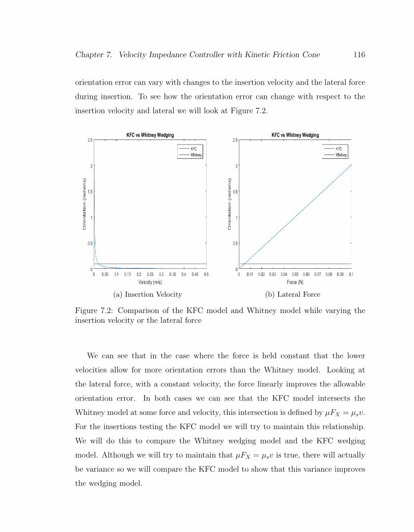
Chapter 7. Velocity Impedance Controller with Kinetic Friction Cone 116
orientation error can vary with changes to the insertion velocity and the lateral force
during insertion. To see how the orientation error can change with respect to the
insertion velocity and lateral we will look at Figure 7.2.
(a) Insertion Velocity (b) Lateral Force
Figure 7.2: Comparison of the KFC model and Whitney model while varying theinsertion velocity or the lateral force
We can see that in the case where the force is held constant that the lower
velocities allow for more orientation errors than the Whitney model. Looking at
the lateral force, with a constant velocity, the force linearly improves the allowable
orientation error. In both cases we can see that the KFC model intersects the
Whitney model at some force and velocity, this intersection is defined by µFX = µsv.
For the insertions testing the KFC model we will try to maintain this relationship.
We will do this to compare the Whitney wedging model and the KFC wedging
model. Although we will try to maintain that µFX = µsv is true, there will actually
be variance so we will compare the KFC model to show that this variance improves
the wedging model.

Chapter 7. Velocity Impedance Controller with Kinetic Friction Cone 117
7.1.2 Kinetic Friction Jamming Model
We will again compare the difference in the jamming model between the KFC and
the Whitney model. For the jamming model’s force relationship, we first get the
relationship between the lateral and insertion force FxFz
< Fxµsv
. From this we get a
familiar requirement to prevent jamming Fz > µsv, which ensures that equation
(7.3) is true at even the lowest allowable velocity, vmin. We see that we have the
same upper bound relationship as the wedging model. The following equation shows
the difference between the jamming parameter for the KFC model and the Whitney
model.
(a) Insertion Velocity (b) Lateral Force
Figure 7.3: Comparison of the KFC model and Whitney model while varying theinsertion velocity or the lateral force

Chapter 7. Velocity Impedance Controller with Kinetic Friction Cone 118
λKFC =Fxz
µsvD
λWhitney =z
µD(7.7)
Similar to equation (7.6) we see that the jamming parameter will behave similar
to the wedging. Figure 7.3 shows this relationship between the KFC and the Whitney
jamming parameter. From Figure 7.3 we see the same type of profile for how the
jamming parameter varies for insertions velocities and lateral forces. We also see
that the jamming parameter has the same intersection point between the Whitney
and KFC model where µFX = µsv. This means that now the impedance controllers
now have two methods of preventing jamming. The controller can now vary the
compliance to minimize MrFz
or also control the insertion velocity and lateral force.
7.1.3 Kinetic Friction Cone Compliance Model
The Whitney model for insertion assumes quasi-static force interaction. We will
impose an extra kinetic friction constraint. In particular we will set the kinetic
friction to be approximately the same as the static friction force. From Figures 7.2
and 7.3 this is the point where the KFC model intersects the Whitney model.
µFx ≈ µsv (7.8)
Equation (7.6) can be rewritten as Fx ≈ µsvµ
. By setting this constraint we can
preserve the Whitney jamming model. To relate this back to the reaction forces the
robot and peg would expect to experience from the insertion we have to split the
analysis into the one-point contact and two-point contact conditions. Once again for

Chapter 7. Velocity Impedance Controller with Kinetic Friction Cone 119
Figure 7.4: Minimum stiffness profile during Cross peg insertion. The blue line isestimating the profile with a constant velocity and the red line is calculating thevelocity.
both stages we have a predetermined KθKx
. Finding the control stiffness for the one
point contact we will combine (4.21) with Fz > µsv.
Kx >µsv
µ[KxKθ
(L− z − µd2
)(L− z) + 1
ε0 − cD2
+ lθ0] (7.9)
We can see that as the depth increases the stiffness required decreases. Solving
for the stiffness for the two-point contact, we will combine (4.28) and Fz > µsv.
Kx >µsva
(7.10)
a =2µ
z[(L2 +
Kθ
Kx
) (θ0 − cDz
) + L(ε0 + cD2
)] + µ(1 + µdz
)[−L(θ0 − cDz
)− (ε0 + cD2
)]
(7.11)

Chapter 7. Velocity Impedance Controller with Kinetic Friction Cone 120
For this model we will look at the differences when we treat v as constant vs.
when it is used as a variable for insertion. To do this we will take an insertion
profile from one of the previous insertions, in particular the cross insertion for the
velocity impedance controller. Figure 7.4 shows the minimum stiffness needed for
the kinetic friction model. Here we compare the response using a constant velocity
model with dynamically calculating the velocity during the insertion. From Figure
7.4, we can see that the constant velocity profile is either very close to the actual
velocity profile or larger than the actual profile. The profile we are calculating is
the minimum stiffness required for a successful insertion. For our insertions we will
be using compliance parameters much larger than these values so we do not need to
worry about jamming.
Figure 7.5: Stiffness profile during insertion.
This explains why there is no jamming in all of the insertions for both impedance
controllers. The largest value from the minimum required stiffness profile during the
two point contact is about KX ≈ 475Nm
. Since all insertions were done well above

Chapter 7. Velocity Impedance Controller with Kinetic Friction Cone 121
this value, with the insertion stiffness set at KX = 500Nm
, we never saw any jamming
issues after the initial point of contact. For insertion testing using this compliance
model we will use the same profile as the minimum stiffness profile. However, we will
be doubling the stiffness values for our controller during the insertion. This stiffness
profile is shown in Figure 7.5
For wedging, we can see that the differences made to the model is the allowable
orientation error, θ < FxcDµsvd
. In the general case we can see that the best wedging
prevention strategy would be to insert as slowly as possible and to provide the most
amount of lateral force. The issue with this strategy is that increasing the lateral force
requires more energy from the robot during insertion. For jamming, we have already
established that jamming will be prevented as long as Fz > µsv. In other words, as
long as the insertion force is larger than the kinetic friction force then increasing the
lateral force during insertion will not cause jamming. Finally we also see that the
jamming parameter, λ = FxzµsvD
, decreases as we increase the insertion velocity and
decrease the lateral force. This means that the likelihood of jamming will increase
as we increase the velocity during insertion. This is the draw back to high speed
insertions, but with an active complaint controller we can vary the compliance during
insertion to prevent jamming. Finally we note that by setting Fx ≈ µsvµ
, the wedging
and jamming parameters return to the same Whitney parameters determined in
chapter 4.
7.2 Insertion Testing with Kinetic Friction Cone
Model
Shown in Figure 7.6 is the kinetic friction cone control model. We will use the
kinetic friction cone restrictions to control the velocity through the path planner
and we will prevent jamming using the kinetic friction compliance parameters. For

Chapter 7. Velocity Impedance Controller with Kinetic Friction Cone 122
Impedance Controller
Robot
Force feedback
IBVS
Task
Velocity
Vision System
Key Inser�onPath Planning
Fric�on Cone
Figure 7.6: Model of kinetic friction cone controller. (KFC-VIC)
the compliance parameters we will complete all of the insertions using the stiffness
values from equations (7.9)-(7.11). To accomplish this we can only use the velocity
impedance controller since the position based impedance controller will lose stability
at these compliance values. We will call this enhanced velocity impedance compliance
controller the kinetic friction cone velocity impedance controller (KFC-VIC) and the
velocity impedance controller (VIC).
To be able to compare the insertion results from the quasi-static model to the
dynamic model we will set the lateral force to Fx ≈ µsvµ
to be able to compare the
difference in the models. When we compare the Whitney wedging model, θ < cDµd
,
with the kinetic friction cone model wedging, θ < FxcDµsvd
, we expect insertions to be
possible when the Whitney model predicts wedging failure. In the Whitney model
we always need the error to be below a set value but for the kinetic friction cone
model the error tolerance can be increased as the insertion velocity and lateral force
vary. This explains why multiple insertions succeeded in chapters 5 and 6 when the

Chapter 7. Velocity Impedance Controller with Kinetic Friction Cone 123
(a) Whitney Model (b) KFC Model
Figure 7.7: Cross peg insertion with KFC-VIC. The top graph is position error, themiddle graph orientation error, and the last graph depth of insertion.The red linescorrespond the Y and θY for the top and bottom graphs, respectively. The blue linecorresponds to the X and θX coordinate. The black lines are the maximum allowablewedging value, Whitney model for (a) and KFC model for (b).
insertions should have failed due to wedging. In this section we will only compare the
velocity impedance controller’s response without the kinetic friction cone compliance
and with its compliance model. This will show that the Whitney model predicts a
failure when the insertion will actually succeed. We will also display the KFC wedging
model during these insertions to display how the insertions are able to succeed.
7.2.1 Cross Insertion
First, let us look at the error response between the Whitney and the KFC wedging
model. Figure 7.7 shows the response of the cross insertion for the KFC-VIC and
Figure 7.8 shows the response for the VIC. In both figures we see that the KFC

Chapter 7. Velocity Impedance Controller with Kinetic Friction Cone 124
(a) Whitney Model (b) KFC Model
Figure 7.8: Cross peg insertion with VIC. The top graph is position error, the middlegraph orientation error, and the last graph depth of insertion.The red lines correspondthe Y and θY for the top and bottom graphs, respectively. The blue line correspondsto the X and θX coordinate. The black lines are the maximum allowable wedgingvalue, Whitney model for (a) and KFC model for (b)
model only intersects with the error at a few points during the insertion. In Figure
7.7 we see that the Whitney model has multiple points in the orientation error where
the insertion should fail whereas the KFC model barely intersects at this point. In
Figure 7.8 we see that the Whitney model has a better initial model of the error,
as the insertion does not begin until the error drops below this threshold. This is
due to the fact that at the beginning of the insertion the peg is hardly moving and
this would make the allowable error to become incredibly large, as shown in Figure
7.2(a).
The first noticeable difference between the controllers is how the KFC-VIC has
multiple points where the error is greater than the maximum wedging error predicted
by the Whitney model. This shows that while we increase the velocity of the insertion

Chapter 7. Velocity Impedance Controller with Kinetic Friction Cone 125
(a) KFC-VIC (b) Velocity Impedance Controller
Figure 7.9: Cross peg jamming response. The black line is the modeled maximumjamming parameter and the blue line is the jamming response.
we also increase the position and orientation error.
In Figure 7.9 we see the jamming response generated by both controllers. As
we have seen in all insertions for both the position based impedance controller and
the velocity impedance controllers and again in Figure 7.9, there is no noticeable
jamming response when compared to the maximum allowable jamming parameter,
the black line in Figure 7.9. This is very important because increasing the velocity
also increases the likelihood for jamming, as shown in Figure 7.3 (a). Both compliance
models are good enough to prevent causes for concern with jamming. For the rest
of the insertions we will not look at the jamming responses since the compliance
controllers significantly reduces the likelihood of failure from jamming.
In Figure 7.10 we compare the experimental insertion force to the modeled inser-
tion force. The profiles of the actual insertion forces are very similar between the two
controllers. The kinetic friction cone model has a larger error but this is mostly due

Chapter 7. Velocity Impedance Controller with Kinetic Friction Cone 126
(a) KFC-VIC (b) Velocity Impedance Controller
Figure 7.10: Cross peg insertion force. The black line is the modeled insertion forcewhile blue line is the actual response.
to the fact that this insertion force model uses the Whitney insertion force model.
This means that there are dynamic responses from the reaction forces during inser-
tion not modeled, such as damping forces from the robot and the environment. This
also explains why the initial insertion force response closely resembles the Whitney
model as the velocities are small enough where kinetic friction force starts to become
µFX = µsv.
Based on Figures 7.7 and 7.8 we can see that the the KFC model predicts suc-
cessful insertions even when the Whitney model predicts the insertion to fail. The
caveat is that this requires the robot to push against the environment more than the
regular model. For the position based impedance controller this additional force to
the environment will likely cause the controller to become unstable which makes the
KFC model only possible with the velocity impedance controller.

Chapter 7. Velocity Impedance Controller with Kinetic Friction Cone 127
(a) Whitney Model (b) KFC Model
Figure 7.11: Cross peg insertion against gravity for KFC-VIC. The top graph is posi-tion error, the middle graph orientation error, and the last graph depth of insertion.The red lines correspond the Z and θZ for the top and bottom graphs, respectively.The blue line corresponds to the X and θX coordinate. The black lines are themaximum allowable wedging value, Whitney model for (a) and KFC model for (b)
7.2.2 Cross Insertion Against Gravity
Now let us look at the error response from the cross insertion acting against gravity,
Figures 7.11 and 7.12 shows this error response for the cross peg insertion against
gravity. In both figures we see that the KFC models the wedging failure threshold
better than the Whitney model. We also see that the KFC-VIC has much larger
errors than the VIC again.
As in the previous insertion, we see the KFC-VIC has significant error during the
insertion, which should cause it to fail. We also have similar insertion profiles from
the previous cross insertion with the velocity impedance controller. Again we see
from the KFC model, the insertion is able to be successful even with errors where

Chapter 7. Velocity Impedance Controller with Kinetic Friction Cone 128
(a) Whitney Model (b) KFC Model
Figure 7.12: Cross peg insertion against gravity for VIC. The top graph is positionerror, the middle graph orientation error, and the last graph depth of insertion. Thered lines correspond the Z and θZ for the top and bottom graphs, respectively. Theblue line corresponds to the X and θX coordinate. The black lines are the maximumallowable wedging value, Whitney model for (a) and KFC model for (b)
the Whitney model predicts wedging failure.
Figure 7.13 shows the insertion force response for cross peg insertion against
gravity. For this insertion the KFC-VIC is more similar to the insertion model than
the VIC. As was the case for the position based impedance controller, both insertion
forces settle at much larger values than those predicted by the Whitney insertion
force model. This is likely due to the gravity acting on the peg because gravity
causes the peg to experience an additional moment and force not modeled in the
Whitney model. We also see that the insertion force required for the KFC-VIC for
this insertion is still larger than the velocity impedance controller.

Chapter 7. Velocity Impedance Controller with Kinetic Friction Cone 129
(a) KFC-VIC (b) Velocity Impedance Controller
Figure 7.13: Cross peg insertion force against gravity. The black line is the modeledinsertion force while blue line is the actual response.
7.2.3 Key Insertion
The final insertion we will compare for the KFC model is the key insertion. Figures
7.14 and 7.15 show the errors from the experimental response for the key insertion.
For this insertion we see a few points where the error intersects with the maximum
allowable wedging value. There is a point where the KFC-VIC passes the error
threshold and the insertion still continues for the KFC model. We see the KFC
model has multiple points of intersection for the VIC. Interesting enough the last
points where the error intersects with the KFC model the insertion hastens. In
the Whitney model, we see that the insertions begin when the errors fall below the
Whitney models threshold. The insertion velocity for this experiment is low enough
where the Whitney model is the more accurate model.
Figure 7.16 shows the insertion force responses during key insertion. In this image

Chapter 7. Velocity Impedance Controller with Kinetic Friction Cone 130
(a) Whitney Model (b) KFC Model
Figure 7.14: Key insertion for the KFC-VIC. The top graph is position error, themiddle graph orientation error, and the last graph depth of insertion. The red linescorrespond the Y and θY for the top and bottom graphs, respectively. The blue linecorresponds to the Z and θZ coordinate. The black lines are the maximum allowablewedging value, Whitney model for (a) and KFC model for (b)
we see the initial insertion force response is similar in both responses. The KFC-VIC
is again closer to the insertion model. Both responses settle at a larger value than
the Whitney model due to the gravity acting on the key. Finally we also see that
the insertion force required for the KFC-VIC is about 3 times as much as the VIC.
These three insertion responses have shown that the KFC model does increase the
allowable error for successful insertion when the velocity is large enough for the quasi-
static assumption to break down. We saw that at lower velocities, where the quasi-
static assumption can remain true, the Whitney model is a more accurate wedging
model. The issue with increasing the velocity during insertion is that all three KFC-
VIC responses have produced larger, but comparable, errors than the normal velocity
impedance controller method. We also see that the KFC-VIC requires a much larger

Chapter 7. Velocity Impedance Controller with Kinetic Friction Cone 131
(a) Whitney Model (b) KFC Model
Figure 7.15: Key insertion for the VIC. The top graph is position error, the middlegraph orientation error, and the last graph depth of insertion. The red lines cor-respond the Y and θY for the top and bottom graphs, respectively. The blue linecorresponds to the Z and θZ coordinate. The black lines are the maximum allowablewedging value, Whitney model for (a) and KFC model for (b)
insertion force than the standard insertion method. This increased insertion force
can cause the position based impedance controller to become unstable. From these
results we see that the KFC model does increase the allowable orientation error to
prevent wedging. We also saw that increasing the velocity will decrease the jamming
parameter but any compliance controller will be enough to prevent jamming. In
turn, using the kinetic friction cone compliance model for insertion will provide more
reliable insertions with the larger threshold for orientation error.

Chapter 7. Velocity Impedance Controller with Kinetic Friction Cone 132
(a) KFC-VIC (b) Velocity Impedance Controller
Figure 7.16: Key insertion force. The black line is the modeled insertion force whileblue line is the actual response.
7.3 Summary
From the KFC model, we saw that at velocities where µFX < µsv the KFC model
better predicts the orientation tolerance for wedging. At velocities below this thresh-
old we saw that the Whitney model was reliable and better modeled the orientation
tolerance. This is due to the fact that at these lower velocities we can use the
quasi-static assumption. We also saw that the jamming tolerance would decrease as
we increased the insertion velocities but this was never an issue as our compliance
controllers effectively prevent jamming.
We noticed that the KFC-VIC insertion force response was more similar to the
Whitney model than the response of the VIC. The main difference is that all of the
insertion forces from the KFC-VIC are much larger than the insertion forces from
the VIC.

Chapter 7. Velocity Impedance Controller with Kinetic Friction Cone 133
From these results we saw that the KFC-VIC provides a closer insertion profile
to what we expect. We also saw that the KFC-VIC has faster insertions than the
VIC. The issue with the KFC-VIC is that it also generates larger position and pose
errors than the VIC. The KFC-VIC also demands higher insertion forces than the
VIC. From these results the benefit to using the KFC-VIC is that the insertion forces
will be closer to the expected value and that the insertions will be faster.
From the kinetic friction cone model results, we saw that as we increase the veloc-
ity we need to increase the lateral force to ensure we have a large enough orientation
tolerance. Regarding the position impedance controller we know that increasing this
lateral force during insertion will likely cause it to become unstable. We did see that
the position impedance controller has the smaller initial errors than the VIC. This
implies that the position impedance controller is a preferable impedance controller
to use for insertions at lower velocities where the Whitney model is still accurate.
However, for high speed insertions, which are clearly advantageous, the KFC-VIC is
the preferred controller due to its insertion and compliance model.
From these results we see that using the kinetic friction cone model for insertion
modeling improves the accuracy in the allowable wedging and jamming for the inser-
tion. We saw that this model falls apart when µFX > µsv and the Whitney model
is the better insertion model at these lower velocities. We also saw that the kinetic
friction cone compliance controller, KFC-VIC, improves the insertion force and the
rate of insertion. However, we saw an increase in position and pose error and that
the insertion requires a larger insertion force than the velocity impedance controller.

134
Chapter 8
Conclusion
In this thesis we introduced a new compliance controller to rival the well-known po-
sition impedance controller. We compared the stability of the two controllers and
demonstrated the response of both controllers with the inclusion of a vision controller
to improve both impedance controllers accuracy. We then tested both controllers’
response to various insertion geometries in various configurations. While the posi-
tion impedance controller has the faster and slightly more accurate response at the
same stiffness values as the velocity impedance controller, the velocity impedance
controller has a larger range of stability with respect to higher stiffness values . The
velocity impedance controller also stays stable when interacting with high stiffness
environments. During the insertion experiments we saw the limitations of using the
position impedance controller at higher stiffness values with respect to stability.
We also introduced the idea of kinetic friction cone compliance model to improve
upon insertions for the velocity impedance controller. We saw that the velocity
impedance controller was capable of using the kinetic friction model due to its larger
range of stability, whereas the position impedance controller would become unstable.
This is because of the larger insertions forces required for the kinetic friction cone
model which was found to be three to fives times larger than the normal insertion

Chapter 8. Conclusion 135
force. We saw that KFC-VIC was capable of successful insertions for errors that
would cause wedging. From these results we can conclude that the proposed velocity
based visual impedance controller is a viable compliance controller with the bene-
fit of having more stability at higher stiffness values than the position impedance
controller.
Another important aspect of the velocity based visual impedance controller is
that the compliance can also be controlled using the damping parameters. These
damping control responses were not explored in this thesis work since the position
impedance controller was not able to reliably vary these parameters. As we needed
to compare the improvements using the velocity impedance controller over using
the position based impedance controller we needed to compare the two controllers
using the same compliance values. Since this work has shown the difference of the
velocity and position based impedance controllers while using similar parameters,
future research would look at the improvement of the compliance model by including
the damping response into the model. By including the damping as an active force
into the compliance model we can further extend the kinetic friction cone compliance
model and model additional dynamic insertion forces. By doing this it may be
possible to develop a dynamic controllable object insertion model.

136
References
[1] N. Andreff, R. Horaud, and B. Espiau. On-line hand-eye calibration. In Proceed-ings. Second International Conference on 3-D Digital Imaging and Modeling,,pages 430–436, 1999.
[2] S. Babaci, Y. Amirat, J. Pontnau, and C. Francois. Fuzzy adaptation impedanceof a 6 dof parallel robot: application to peg in hole insertion. In Fuzzy Systems,1996., Proceedings of the Fifth IEEE International Conference on, volume 3,pages 1770–1776 vol.3, Sep 1996.
[3] A. Becker, C. Ertel, and J. McLurkin. Crowdsourcing swarm manipulationexperiments: A massive online user study with large swarms of simple robots.In 2014 IEEE International Conference on Robotics and Automation (ICRA),pages 2825–2830, May 2014.
[4] F. Chaumette. Visual servoing. In K. Ikeuchi, editor, Computer Vision: AReference Guide, pages 869–874. Springer, 2014.
[5] Chao-Jen Chen, Ming-Yang Cheng, and Ke-Han Su. Observer-based impedancecontrol and passive velocity control of power assisting devices for exercise andrehabilitation. In Industrial Electronics Society, IECON 2013 - 39th AnnualConference of the IEEE, pages 6502–6507, Nov 2013.
[6] M. Erdmann. A configuration space friction cone. In Intelligent Robotsand Systems ’91. ’Intelligence for Mechanical Systems, Proceedings IROS ’91.IEEE/RSJ International Workshop on, pages 455–460 vol.2, Nov 1991.
[7] B. Espiau, F. Chaumette, and Patrick Rives. A new approach to visual servoingin robotics. Robotics and Automation, IEEE Transactions on, 8(3):313–326,1992.
[8] S. E. Everett, T. F. Chan, and R. V. Dubey. Diagonalization of telerobotic handcontroller impedance for accurate force and velocity transmission. In Robotics

References 137
and Automation, 1997. Proceedings., 1997 IEEE International Conference on,volume 3, pages 2198–2203 vol.3, Apr 1997.
[9] Cheng Gao, Xingzhe Piao, and Weiyan Tong. Optimal motion control for ibvsof robot. In Intelligent Control and Automation (WCICA), 2012 10th WorldCongress on, pages 4608–4611, July 2012.
[10] M. Gendrin, J. Y. Gauthier, and X. Lin-Shi. An impedance control using a finitecontrol set model predictive controller. In 2015 IEEE International Symposiumon Predictive Control of Electrical Drives and Power Electronics (PRECEDE),pages 85–90, Oct 2015.
[11] M. Gilli and Pastorelli S. Lumia, R. Precision robotic assembly using attractiveregions. In International Journal of Recent Advances in Mechanical Engineering,volume 3, pages 109–128, August 2014.
[12] K. P. Hawkins, S. Bansal, N. N. Vo, and A. F. Bobick. Anticipating hu-man actions for collaboration in the presence of task and sensor uncertainty.In 2014 IEEE International Conference on Robotics and Automation (ICRA),pages 2215–2222, May 2014.
[13] C Ho, C Basdogan, and M Srinivasan. Efficient point-based rendering techniquesfor haptic display of virtual objects. Presence, 8(5):477–491, Oct 1999.
[14] N. Hogan. Impedance control: An approach to manipulation. In AmericanControl Conference, 1984, pages 304–313, June 1984.
[15] Seung kook Yun. Compliant manipulation for peg-in-hole: Is passive compliancea key to learn contact motion? In Robotics and Automation, 2008. ICRA 2008.IEEE International Conference on, pages 1647–1652, May 2008.
[16] D. Kotake, S. Uchiyama, and H. Yamamoto. A marker calibration methodutilizing a priori knowledge on marker arrangement. In Mixed and AugmentedReality, 2004. ISMAR 2004. Third IEEE and ACM International Symposiumon, pages 89–98, Nov 2004.
[17] X. Lamy, F. Colledani, and P. O. Gutman. Identification and experimentationof an industrial robot operating in varying-impedance environments. In Intel-ligent Robots and Systems (IROS), 2010 IEEE/RSJ International Conferenceon, pages 3138–3143, Oct 2010.
[18] F. Lange, M. Frommberger, and G. Hirzinger. Impedance-based smoothing forvisual servoing along edges. In Joint Conference on Roboticvs, January 2006.

References 138
[19] B. Lara, K. Althoefer, and L.D. Seneviratne. Automated robot-based screw in-sertion system. In Industrial Electronics Society, 1998. IECON ’98. Proceedingsof the 24th Annual Conference of the IEEE, volume 4, pages 2440–2445 vol.4,Aug 1998.
[20] D. A. Lawrence. Impedance control stability properties in common implementa-tions. In Robotics and Automation, 1988. Proceedings., 1988 IEEE InternationalConference on, pages 1185–1190 vol.2, Apr 1988.
[21] M. Lendermann, B. R. P. Singh, F. Stuhlenmiller, P. Beckerle, S. Rinderknecht,and P. V. Manivannan. Comparison of passivity based impedance controllerswithout torque-feedback for variable stiffness actuators. In 2015 IEEE Inter-national Conference on Advanced Intelligent Mechatronics (AIM), pages 1126–1131, July 2015.
[22] V. Lippiello, B. Siciliano, and L. Villani. A position-based visual impedancecontrol for robot manipulators. In Robotics and Automation, 2007 IEEE Inter-national Conference on, pages 2068–2073, April 2007.
[23] A.R Locks. Cylinder locks, 2015.
[24] B. Maldonado, M. Mendoza, I. Bonilla, and I. Reyna-Gutirrez. Stiffness-basedtuning of an adaptive impedance controller for robot-assisted rehabilitation ofupper limbs. In 2015 37th Annual International Conference of the IEEE Engi-neering in Medicine and Biology Society (EMBC), pages 3578–3581, Aug 2015.
[25] M.T. Mason. Complaint Motion. MIT Press, 1983.
[26] Wim Meeussen, M. Wise, S. Glaser, S. Chitta, C. McGann, P. Mihelich,E. Marder-Eppstein, M. Muja, Victor Eruhimov, T. Foote, J. Hsu, R.B. Rusu,B. Marthi, G. Bradski, K. Konolige, B. Gerkey, and E. Berger. Autonomousdoor opening and plugging in with a personal robot. In Robotics and Automation(ICRA), 2010 IEEE International Conference on, pages 729–736, May 2010.
[27] D. Meike, M. Pellicciari, and G. Berselli. Energy efficient use of multirobotproduction lines in the automotive industry: Detailed system modeling andoptimization. IEEE Transactions on Automation Science and Engineering,11(3):798–809, July 2014.
[28] TH. Meitinger and F. Pfeiffer. The spatial peg-in-hole problem. In IEEE/RSJCong. on Intelligent Robots & Systems, pages 54–59, 1995.
[29] N. Melder and W.S. Harwin. Improved rendering for multi-finger manipulationusing friction cone based god-objects. In Proc. Eurohaptics Conference, pages82–85, 2003.

References 139
[30] N. Melder and W.S. Harwin. Extending the friction cone algorithm for arbitrarypolygon based haptic objects. In Haptic Interfaces for Virtual Environmentand Teleoperator Systems, 2004. HAPTICS ’04. Proceedings. 12th InternationalSymposium on, pages 234–241, March 2004.
[31] H.B Morgenbesser and M.A. Srinivasan. Force shading and bump mapping usingthe friction cone algorithm. In Proceedings of the ASME Dynamics Systems andControl Division, volume 58, pages 407–412, 1996.
[32] Y. Nakabo and M. Ishikawa. Visual impedance using 1 ms visual feedback sys-tem. In Robotics and Automation, 1998. Proceedings. 1998 IEEE InternationalConference on, volume 3, pages 2333–2338 vol.3, May 1998.
[33] B.J. Nelson, J.D. Morrow, and P.K. Khosla. Improved force control throughvisual servoing. In American Control Conference, Proceedings of the 1995, vol-ume 1, pages 380–386 vol.1, Jun 1995.
[34] V. Nevarez and R. Lumia. Image jacobian estimation using structure frommotion on a centralized point. In Intelligent Robots and Systems (IROS 2014),2014 IEEE/RSJ International Conference on, pages 773–778, Sept 2014.
[35] E. Nichols and W. Franklin. The Elements of Physics. Macmillan, 1898.
[36] R. Oboe and D. Pilastro. Stability analysis of a non-linear adaptive impedancecontroller for rehabilitation purposes. In Mechatronics (ICM), 2015 IEEE In-ternational Conference on, pages 454–459, March 2015.
[37] S. Oh and Y. Hori. Fractional order impedance control by particle swarm op-timization. In Control, Automation and Systems, 2008. ICCAS 2008. Interna-tional Conference on, pages 1936–1941, Oct 2008.
[38] M.D. O’Leary, C. Simone, T. Washio, K. Yoshinaka, and A.M. Okamura.Robotic needle insertion: effects of friction and needle geometry. In Roboticsand Automation, 2003. Proceedings. ICRA ’03. IEEE International Conferenceon, volume 2, pages 1774–1780 vol.2, Sept 2003.
[39] F. Parietti and H. H. Asada. Supernumerary robotic limbs for aircraft fuselageassembly: Body stabilization and guidance by bracing. In 2014 IEEE Interna-tional Conference on Robotics and Automation (ICRA), pages 1176–1183, May2014.
[40] F. Parietti, K. Chan, and H. H. Asada. Bracing the human body with supernu-merary robotic limbs for physical assistance and load reduction. In 2014 IEEEInternational Conference on Robotics and Automation (ICRA), pages 141–148,May 2014.

References 140
[41] M. Pelletier and M. Doyon. On the implementation and performance ofimpedance control on position controlled robots. In Robotics and Automation,1994. Proceedings., 1994 IEEE International Conference on, pages 1228–1233vol.2, May 1994.
[42] M.A. Peshkin. Programmed compliance for error corrective assembly. Roboticsand Automation, IEEE Transactions on, 6(4):473–482, Aug 1990.
[43] J. Pomares, G. J. Garcia, L. Paya, and F. Torres. Adaptive visual servoingand force control fusion to track surfaces. In Proceedings of the 2005 WSEASInternational Conference on Dynamical Systems and Control, volume 5, January2006.
[44] J. Pomares, G. J. Garcia, and F. Torres. Impedance control for fusing mul-tisensorial systems in robotic manipulation tasks. In Proceedings of the 2005WSEAS International Conference on Dynamical Systems and Control, pages357–362, Stevens Point, Wisconsin, USA, 2005. World Scientific and Engineer-ing Academy and Society (WSEAS).
[45] Craig J. J. Raibert, M. H. Hybrid position/force control of manipulators. InASME Journal of Dynamic Systems Measurement and Control, volume 102,pages 126–133, 1981.
[46] C. Richard, M.R. Cutkosky, and K. MacLean. Friction identification for hapticdisplay. In Proceedings of the ASME Dynamics Systems and Control Division,volume 67, November 1999.
[47] L. Roveda, F. Vicentini, N. Pedrocchi, F. Braghin, and L. M. Tosatti. Impedanceshaping controller for robotic applications in interaction with compliant envi-ronments. In Informatics in Control, Automation and Robotics (ICINCO), 201411th International Conference on, volume 02, pages 444–450, Sept 2014.
[48] Kevin Ruybal. A variable compliance controller for cooperative vision guidedrobotic assembly. Master’s thesis, University of New Mexico. Dept. of Mechan-ical Engineering, May 2011.
[49] J.D. Schutter and H.V Brussel. Compliant robot motion i. a formalism for spec-ifying complaint motion tasks. In International Journal of Robotics Research,volume 7, pages 3–17, August 1988.
[50] Y. Shirai and H. Inoue. Guiding a robot by visual feedback in assembling tasks.Pattern Recognition, 5(2):99 – 108, 1973.
[51] J. Simmon. Force Feedback in Robot Assembly Using an Active Wrist withAdaptive Compliance. PhD thesis, Univ. Leuven (Belgium), Dept. of MechanicalEngineering, 1980.

References 141
[52] R.Y. Tsai. A versatile camera calibration technique for high-accuracy 3d ma-chine vision metrology using off-the-shelf tv cameras and lenses. Robotics andAutomation, IEEE Journal of, 3(4):323–344, August 1987.
[53] T. Tsumugiwa, R. Yokogawa, and K. Hara. Variable impedance control withvirtual stiffness for human-robot cooperative peg-in-hole task. In IntelligentRobots and Systems, 2002. IEEE/RSJ International Conference on, volume 2,pages 1075–1081 vol.2, 2002.
[54] T. Watanabe, K. Harada, Zhongwei Jiang, and T. Yoshikawa. Object manipu-lation under hybrid active/passive closure. In Robotics and Automation, 2005.ICRA 2005. Proceedings of the 2005 IEEE International Conference on, pages1013–1020, April 2005.
[55] Daniel E. Whitney. Historical perspective and state of the art in robot forcecontrol. In Robotics and Automation. Proceedings. 1985 IEEE InternationalConference on, volume 2, pages 262–268, Mar 1985.
[56] S. Xiao and Y. Li. Visual servo feedback control of a novel large working rangemicro manipulation system for microassembly. Journal of Microelectromechan-ical Systems, 23(1):181–190, Feb 2014.
[57] Q. Xu. Robust impedance control of a compliant microgripper for high-speed position/force regulation. IEEE Transactions on Industrial Electronics,62(2):1201–1209, Feb 2015.
[58] Q. Zhang and R. Pless. Extrinsic calibration of a camera and laser range finder(improves camera calibration). In Intelligent Robots and Systems, 2004. (IROS2004). Proceedings. 2004 IEEE/RSJ International Conference on, volume 3,pages 2301–2306 vol.3, Sept 2004.
[59] Zhengyou Zhang. Flexible camera calibration by viewing a plane from unknownorientations. In Computer Vision, 1999. The Proceedings of the Seventh IEEEInternational Conference on, volume 1, pages 666–673 vol.1, 1999.
[60] Zhengyou Zhang. A flexible new technique for camera calibration. PatternAnalysis and Machine Intelligence, IEEE Transactions on, 22(11):1330–1334,Nov 2000.
[61] Zhuyingqingfen. Firction approximation, 2014.