a3 · chapter 38 a3 1. introduction 39 2. three phase fault calculations 39 3. symmetrical...

A3

Schneider Electric - Network Protection & Automation Guide37

Fault Calculations

A3 Fault Calculations

Network Protection & Automation Guide

Fault Calculations

Chapter

38

A31. Introduction 39

2. Three phase fault calculations 39

3. Symmetrical component analysis of a three-phase network 41

4. Equations and network connections for various types of faults 43

5. Current and voltage distribution in a system due to a fault 47

6. Effect of system earthing on zero sequence quantities 50

7. References 54

Network Protection & Automation Guide

Fault Calculations

A3


Fault Calculations

point F are Z'1 and Z''1, and the current through point F before the fault occurs is I .

The voltage V at F before fault inception is:

Z''V Z''= +=- E''E I I

After the fault the voltage V is zero. Hence, the change in voltage is -V . Because of the fault, the change in the current flowing into the network from F is:

∆I VZ

VZ Z

Z Z= − = −

+( )1

1 1

1 1

' ''

' ' '

and, since no current was flowing into the network from F prior to the fault, the fault current flowing from the network into the fault is:

A power system is normally treated as a balanced symmetrical three-phase network. When a fault occurs, the symmetry is normally upset, resulting in unbalanced currents and voltages appearing in the network. The only exception is the three-phase fault, which, because it involves all three phases equally at the same location, is described as a symmetrical fault. By using symmetrical component analysis and replacing the normal system sources by a source at the fault location, it is possible to analyse these fault conditions.

For the correct application of protection equipment, it is essential to know the fault current distribution throughout the system and the voltages in different parts of the system due to the fault. Further, boundary values of current at any relaying point must be known if the fault is to be cleared with discrimination.

1. Introduction

The information normally required for each kind of fault at each relaying point is:

a. maximum fault current

b. minimum fault current

c. maximum through fault current

To obtain the above information, the limits of stable generation and possible operating conditions, including the method of system earthing, must be known. Faults are always assumed to be through zero fault impedance.

2. Three-phase fault calculations

Three-phase faults are unique in that they are balanced, that is, symmetrical in the three phases, and can be calculated from the single-phase impedance diagram and the operating conditions existing prior to the fault.

A fault condition is a sudden abnormal alteration to the normal circuit arrangement. The circuit quantities (current and voltage) will alter, and the circuit will pass through a transient state to a steady state. In the transient state, the initial magnitude of the fault current will depend upon the point on the voltage wave at which the fault occurs. The decay of the transient condition, until it merges into steady state, is a function of the parameters of the circuit elements. The transient current may be regarded as a d.c. exponential current superimposed on the symmetrical steady state fault current. In a.c. machines, owing to armature reaction, the machine reactances pass through ‘sub transient’ and ‘transient’ stages before reaching their steady state synchronous values. For this reason, the resultant fault current during the transient period, from fault inception to steady state also depends on the location of the fault in the network relative to that of the rotating plant.

In a system containing many voltage sources, or having a complex network arrangement, it is tedious to use the normal system voltage sources to evaluate the fault current in the faulty branch or to calculate the fault current distribution in the system. A more practical method [Ref A3.1: Circuit Analysis of A.C. Power Systems] is to replace the system voltages by a single driving voltage at the fault point. This driving voltage is the voltage existing at the fault point before the fault occurs.

Consider the circuit given in Figure A3.1 where the driving voltages are E' and E'' , the impedances on either side of fault

N

F

Figure A3.1:Network with fault at F

A3

Schneider Electric - Network Protection & Automation Guide 40

Fault Calculations

I f I VZ Z

Z Z= − =

+( )∆ 1 1

1 1

' ''

' ' '

By applying the Principle of Superposition, the load currents circulating in the system prior to the fault may be added to the currents circulating in the system due to the fault, to give the total current in any branch of the system at the time of fault inception. However, in most problems, the load current is small in comparison to the fault current and is usually ignored.

In a practical power system, the system regulation is such that the load voltage at any point in the system is within 10% of the declared open-circuit voltage at that point. For this reason, it is usual to regard the pre-fault voltage at the fault as being the open-circuit voltage, and this assumption is also made in a number of the standards dealing with fault level calculations.

For an example of practical three-phase fault calculations, consider a fault at A in Figure A2.9. With the network reduced as shown in Figure A3.2, the load voltage at A before the fault occurs is:

V = +E'0.97 1.55 I

V = + +E''0.99 1.2 x 2.52.5 + 1.2 0.39 I

For practical working conditions, >>>E' 1.55 I and >>>E'' 1.207I . Hence =~ =~E' E'' V .

Replacing the driving voltages E'' and E'' by the load voltage V between A and N modifies the circuit as shown in Figure A3.3(a).

The node A is the junction of three branches. In practice, the node would be a busbar, and the branches are feeders radiating from the bus via circuit breakers, as shown in Figure A3.3(b). There are two possible locations for a fault at A; the busbar side of the breakers or the line side of the breakers. In this example, it is assumed that the fault is at X, and it is required to calculate the current flowing from the bus to X.


N

1.55 ΩA B

2.5 Ω

1.2 Ω

0.39 Ω

0.990.97

Figure A3.2:Reduction of typical power system network

The network viewed from AN has a driving point impedance Z1 = 0.68 Ω.

The current in the fault is VZ1

.

Let this current be 1.0 per unit. It is now necessary to find the fault current distribution in the various branches of the network and in particular the current flowing from A to X on the assumption that a relay at X is to detect the fault condition. The equivalent impedances viewed from either side of the fault are shown in Figure A3.4(a).

The currents from Figure A3.4(a) are as follows:

From the right: 1.552.76

= 0.563 p.u.

From the left: 1.212.76

= 0.437 p.u.

There is a parallel branch to the right of A

Therefore, current in 2.5 ohm branch

1.2 x 0.5633.7

== 0.183 p.u.

N

A

V

B

A

X

(b) Typical physical arrangement of node A with a fault shown at X

(a) Three - phase fault diagram for a fault at node A

BusbarCircuit breaker

1.55Ω

1.2Ω

2.5Ω

0.39Ω

Figure A3.3:Network with fault at node A

A3


Fault Calculations


and the current in 1.2 ohm branch

2.5 x 0.5633.7

== 0.38 p.u.

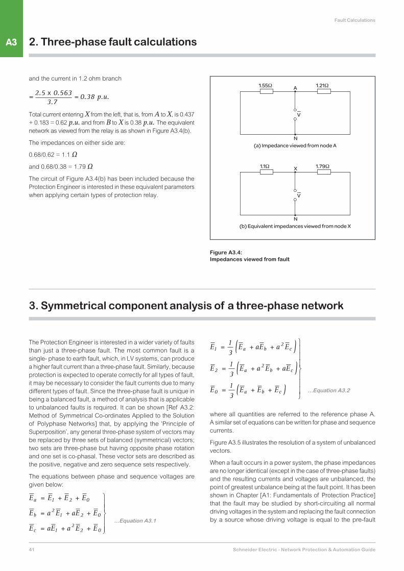
Total current entering X from the left, that is, from A to X, is 0.437 + 0.183 = 0.62 p.u. and from B to X is 0.38 p.u. The equivalent network as viewed from the relay is as shown in Figure A3.4(b).

The impedances on either side are:

0.68/0.62 = 1.1 Ω

and 0.68/0.38 = 1.79 Ω

The circuit of Figure A3.4(b) has been included because the Protection Engineer is interested in these equivalent parameters when applying certain types of protection relay.

N

V

A

N

V

X

1.55Ω 1.21Ω

1.79Ω1.1Ω

(a) Impedance viewed from node A

(b) Equivalent impedances viewed from node X

Figure A3.4:Impedances viewed from fault

3. Symmetrical component analysis of a three-phase network

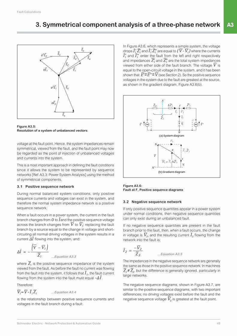
The Protection Engineer is interested in a wider variety of faults than just a three-phase fault. The most common fault is a single- phase to earth fault, which, in LV systems, can produce a higher fault current than a three-phase fault. Similarly, because protection is expected to operate correctly for all types of fault, it may be necessary to consider the fault currents due to many different types of fault. Since the three-phase fault is unique in being a balanced fault, a method of analysis that is applicable to unbalanced faults is required. It can be shown [Ref A3.2: Method of Symmetrical Co-ordinates Applied to the Solution of Polyphase Networks] that, by applying the ‘Principle of Superposition’, any general three-phase system of vectors may be replaced by three sets of balanced (symmetrical) vectors; two sets are three-phase but having opposite phase rotation and one set is co-phasal. These vector sets are described as the positive, negative and zero sequence sets respectively.

The equations between phase and sequence voltages are given below:

E E E E

E a E aE E

E aE a E E

a

b

c

= + +

= + +

= + +

1 2 0

21 2 0

12

2 0

...Equation A3.1

E E aE a E

E E a E aE

E E E E

a b c

a b c

a b c

12

22

0

13

13

13

= + +( )= + +( )= + +( )

...Equation A3.2

where all quantities are referred to the reference phase A. A similar set of equations can be written for phase and sequence currents.

Figure A3.5 illustrates the resolution of a system of unbalanced vectors.

When a fault occurs in a power system, the phase impedances are no longer identical (except in the case of three-phase faults) and the resulting currents and voltages are unbalanced, the point of greatest unbalance being at the fault point. It has been shown in Chapter [A1: Fundamentals of Protection Practice] that the fault may be studied by short-circuiting all normal driving voltages in the system and replacing the fault connection by a source whose driving voltage is equal to the pre-fault

A3


Fault Calculations

voltage at the fault point. Hence, the system impedances remain symmetrical, viewed from the fault, and the fault point may now be regarded as the point of injection of unbalanced voltages and currents into the system.

This is a most important approach in defining the fault conditions since it allows the system to be represented by sequence networks [Ref A3.3: Power System Analysis] using the method of symmetrical components.

3.1 Positive sequence network

During normal balanced system conditions, only positive sequence currents and voltages can exist in the system, and therefore the normal system impedance network is a positive sequence network.

When a fault occurs in a power system, the current in the fault branch changes from 0 to Iand the positive sequence voltage across the branch changes from V to V1; replacing the fault branch by a source equal to the change in voltage and short-circuiting all normal driving voltages in the system results in a current ∆I flowing into the system, and:

∆IV V

Z= −

− )( 1

1 ...Equation A3.3

where Z1 is the positive sequence impedance of the system viewed from the fault. As before the fault no current was flowing from the fault into the system, it follows that I1, the fault current flowing from the system into the fault must equal -∆I .

Therefore:

V = -1 ZV 1I1 ...Equation A3.4

is the relationship between positive sequence currents and voltages in the fault branch during a fault.


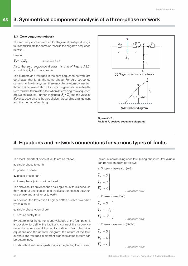
In Figure A3.6, which represents a simple system, the voltage drops I1Z'' 1 and I1Z''' 1 are equal to V )( - 1V where the currentsI1' and I1'' enter the fault from the left and right respectively and impedances Z'1 and Z''1 are the total system impedances viewed from either side of the fault branch. The voltage V is equal to the open-circuit voltage in the system, and it has been shown that E''= =VE' (see Section 2). So the positive sequence voltages in the system due to the fault are greatest at the source, as shown in the gradient diagram, Figure A3.6(b).

3.2 Negative sequence network

If only positive sequence quantities appear in a power system under normal conditions, then negative sequence quantities can only exist during an unbalanced fault.

If no negative sequence quantities are present in the fault branch prior to the fault, then, when a fault occurs, the change in voltage is V2, and the resulting current I2 flowing from the network into the fault is:

I

VZ

22

2= −

...Equation A3.5

The impedances in the negative sequence network are generally the same as those in the positive sequence network. In machines Z1 Z2≠ , but the difference is generally ignored, particularly in large networks.

The negative sequence diagrams, shown in Figure A3.7, are similar to the positive sequence diagrams, with two important differences; no driving voltages exist before the fault and the negative sequence voltage V2 is greatest at the fault point.

Figure A3.5:Resolution of a system of unbalanced vectors N

F

X

Z '1I '1

V1

N

F

N'

X

(a) System diagram

(b) Gradient diagram

Figure A3.6: Fault at F, Positive sequence diagrams

A3


Fault Calculations

3.3 Zero sequence network

The zero sequence current and voltage relationships during a fault condition are the same as those in the negative sequence network.

Hence:

I- 0V =0 Z0 ...Equation A3.6

Also, the zero sequence diagram is that of Figure A3.7, substituting I0 for I2, and so on.

The currents and voltages in the zero sequence network are co-phasal, that is, all the same phase. For zero sequence currents to flow in a system there must be a return connection through either a neutral conductor or the general mass of earth. Note must be taken of this fact when determining zero sequence equivalent circuits. Further, in general Z1 Z0≠ and the value ofZ0 varies according to the type of plant, the winding arrangement and the method of earthing.


(a) Negative sequence networkN

F

X

F

X

N(b) Gradient diagram

Figure A3.7: Fault at F, positive sequence diagrams

4. Equations and network connections for various types of faults

The most important types of faults are as follows:

a. single-phase to earth

b. phase to phase

c. phase-phase-earth

d. three-phase (with or without earth)

The above faults are described as single shunt faults because they occur at one location and involve a connection between one phase and another or to earth.

In addition, the Protection Engineer often studies two other types of fault:

e. single-phase open circuit

f. cross-country fault

By determining the currents and voltages at the fault point, it is possible to define the fault and connect the sequence networks to represent the fault condition. From the initial equations and the network diagram, the nature of the fault currents and voltages in different branches of the system can be determined.

For shunt faults of zero impedance, and neglecting load current,

the equations defining each fault (using phase-neutral values) can be written down as follows:

a. Single-phase-earth (A-E)

I

I

V

b

c

a

=

=

=

0

0

0

...Equation A3.7

b. Phase-phase (B-C)

I

I I

V V

a

b c

b c

=

= −

=

0

...Equation A3.8

c. Phase-phase-earth (B-C-E)

I

V

V

a

b

c

=

=

=

0

0

0 ...Equation A3.9

A3


Fault Calculations

The constraints imposed by Equations A3.15 and A3.17 indicate that there is no zero sequence network connection in the equivalent circuit and that the positive and negative sequence networks are connected in parallel. Figure A3.9 shows the defining and equivalent circuits satisfying the above equations.


d. Three-phase (A-B-C or A-B-C-E)

I I I

V V

V V

a b c

a b

b c

+ + =

=

=

0

...Equation A3.10

It should be noted from the above that for any type of fault there are three equations that define the fault conditions.

When there is a fault impedance, this must be taken into account when writing down the equations. For example, with a single phase-earth fault through fault impedance Zf , Equations A3.7 are re-written:

I

I

V I Z

b

c

a a f

=

=

=

0

0

...Equation A3.11

4.1 Single-phase-earth fault (A-E)

Consider a fault defined by Equations A3.7 and by Figure A3.8(a). Converting Equations A3.7 into sequence quantities by using Equations A3.1 and A3.2, then:

I I I Io a1 213

= = = ...Equation A3.12

+( )-V =1 V2 V0 ...Equation A3.13

Substituting for V1, V2 and V0 in Equation A3.13 from Equations A3.4, A3.5 and A3.6:

+-V =Z1 Z2 Z0I1 I2 I0but, from Equation A3.12, I1 I= 2 I= 0, therefore:

++=V Z( )1 Z2 Z3I1 ...Equation A3.14

The constraints imposed by Equations A3.12 and A3.14 indicate that the equivalent circuit for the fault is obtained by connecting the sequence networks in series, as shown in Figure A3.8(b).

4.2 Phase-phase fault (B-C)

From Equation A3.8 and using Equations A3.1 and A3.2:

I1 I= 2

I1 0= ... Equation A3.15

V1 V2= ... Equation A3.16

From network Equations A3.4 and A3.5, Equation A3.16 can be re-written:

+-V =Z1 Z2 Z0I1 I2 I0-V =Z1 Z2I1 I2

and substituting for I2 from Equation A3.15:

+=V Z( )1 Z2I1 ... Equation A3.17

F

C

B

A

(b) Equivalent circuit

F 1

N1

N2 N0

F 2 F0

(a) Definition of fault

Figure A3.8: Single-phase-earth fault at F


F

C

B

A


F 1

N 1N 2 N 0

F 2 F 0

Figure A3.9:Phase-phase fault at F

A3


Fault Calculations

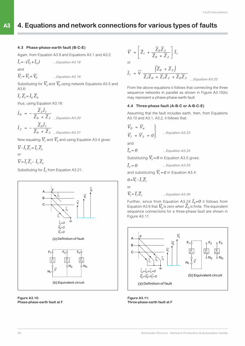
4.3 Phase-phase-earth fault (B-C-E)

Again, from Equation A3.9 and Equations A3.1 and A3.2:

+= -( )I1 I2 I0 ...Equation A3.18

and

V =1 V =2 V0 ...Equation A3.19

Substituting for V2 and V0 using network Equations A3.5 and A3.6:

I =2 Z2 I0 Z0

thus, using Equation A3.18:

IZ I

Z Z0

2 1

0 2= −

+ ...Equation A3.20

IZ I

Z Z2

0 1

0 2= −

+

...Equation A3.21

Now equating V1 and V2 and using Equation A3.4 gives:

-V =Z1 Z2I1 I2or

=V -Z1 Z2I1 I2

Substituting for I2 from Equation A3.21:



F

C

B

A


F1 F2 F0

N0N2

N1

Figure A3.10:Phase-phase-earth fault at F

V ZZ Z

Z ZI= +

+

1

0 2

0 21

or

I VZ Z

Z Z Z Z Z Z1

0 2

1 0 1 2 0 2=

+ )(+ +

...Equation A3.22

From the above equations it follows that connecting the three sequence networks in parallel as shown in Figure A3.10(b) may represent a phase-phase-earth fault.

4.4 Three-phase fault (A-B-C or A-B-C-E)

Assuming that the fault includes earth, then, from Equations A3.10 and A3.1, A3.2, it follows that:

V V

V V

a0

1 2 0

=

= =

...Equation A3.23

and

I0 0= ...Equation A3.24

Substituting V2 0= in Equation A3.5 gives:

I2 0= ...Equation A3.25

and substituting V1 0= in Equation A3.4:

V1 I1Z10= -

or

V1 I1Z1= ...Equation A3.26

Further, since from Equation A3.24 I0=0 it follows from Equation A3.6 that V0 is zero when Z0 is finite. The equivalent sequence connections for a three-phase fault are shown in Figure A3.11.


F

C

B

A


F1 F2 F0

N0N2N1

Figure A3.11:Three-phase-earth fault at F

A3


Fault Calculations


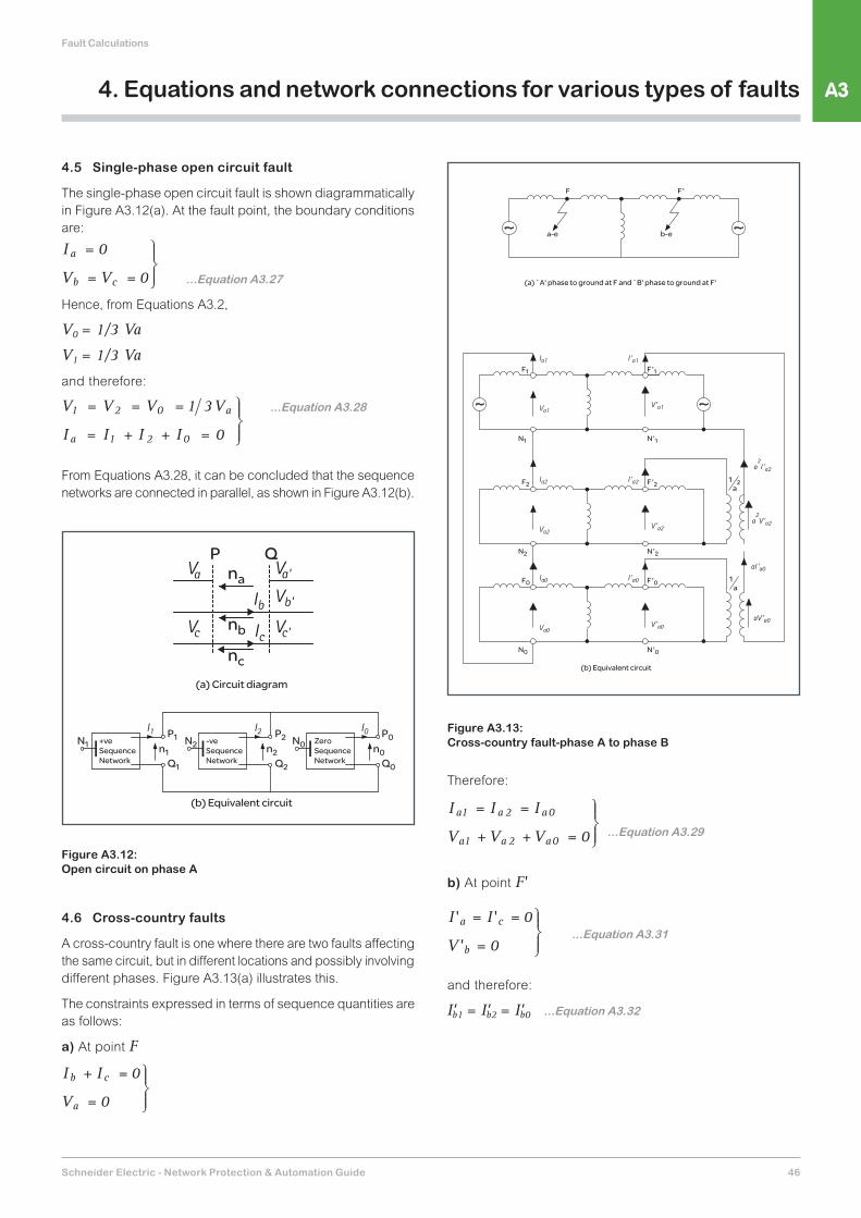
4.5 Single-phase open circuit fault

The single-phase open circuit fault is shown diagrammatically in Figure A3.12(a). At the fault point, the boundary conditions are:

I

V V

a

b c

=

= =

0

0 ...Equation A3.27

Hence, from Equations A3.2,

V0 = 1/3 Va

V1 = 1/3 Va

and therefore:

...Equation A3.28V V V V

I I I I

a

a

1 2 0

1 2 0

1 3

0

= = =

= + + =

From Equations A3.28, it can be concluded that the sequence networks are connected in parallel, as shown in Figure A3.12(b).

4.6 Cross-country faults

A cross-country fault is one where there are two faults affecting the same circuit, but in different locations and possibly involving different phases. Figure A3.13(a) illustrates this.

The constraints expressed in terms of sequence quantities are as follows:

a) At point F

I I

V

b c

a

+ =

=

0

0

Therefore:

I I I

V V V

a a a

a a a

1 2 0

1 2 0 0

= =

+ + =

...Equation A3.29

b) At point F'

...Equation A3.31I I

V

' '

'

a c

b

= =

=

0

0

and therefore:

I'b1 = I'b2 = I'b0 ...Equation A3.32

na

nb

nc

n1N1 N2 N0

P1

Q1

n2

P2

Q2

n0

P0

Q0

P Q

(a) Circuit diagram


+veSequenceNetwork

-veSequenceNetwork

ZeroSequenceNetwork

Figure A3.12:Open circuit on phase A

(a) `A' phase to ground at F and `B' phase to ground at F'

a-e b-e

F 'F


F1 F '1

N1 N '1

F2 F '2

N2 N '2

F0 F '0

N0 N '0

1a

2

1a

Figure A3.13:Cross-country fault-phase A to phase B

A3


Fault Calculations


To solve, it is necessary to convert the currents and voltages at point F' to the sequence currents in the same phase as those at point F. From Equation A3.32,

a2I'a1 = a I'a2 = I'a0

or

I'a1 = a 2I'a2 = a I'a0 ... Equation A3.33

and, for the voltages

V'b1 + V'b2 = V'b0 = 0

Converting:

a 2V'a1 + a V'a2 + V'a0 = 0

or

V'a1 + a 2V'a2 + a V'a0 = 0 ...Equation A3.34

The fault constraints involve phase shifted sequence quantities. To construct the appropriate sequence networks, it is necessary to introduce phase-shifting transformers to couple the sequence networks. This is shown in Figure A3.13(b).

5. Current and voltage distribution in a system due to a fault

Practical fault calculations involve the examination of the effect of a fault in branches of network other than the faulted branch, so that protection can be applied correctly to isolate the section of the system directly involved in the fault. It is therefore not enough to calculate the fault current in the fault itself; the fault current distribution must also be established. Further, abnormal voltage stresses may appear in a system because of a fault, and these may affect the operation of the protection. Knowledge of current and voltage distribution in a network due to a fault is essential for the application of protection.

The approach to network fault studies for assessing the application of protection equipment may be summarised as follows:

a. from the network diagram and accompanying data, assess the limits of stable generation and possible operating conditions for the system

NOTE: When full information is not available assumptions may have to be made

b. with faults assumed to occur at each relaying point in turn, maximum and minimum fault currents are calculated for each type of fault

NOTE: The fault is assumed to be through zero impedance

c. by calculating the current distribution in the network for faults applied at different points in the network (from (b) above) the maximum through fault currents at each relaying point are established for each type of fault

d. at this stage more or less definite ideas on the type of protection to be applied are formed.

Further calculations for establishing voltage variation at the relaying point, or the stability limit of the system with a fault on it, are now carried out in order to determine the class of protection necessary, such as high or low speed, unit or non-unit, etc.

5.1 Current distribution

The phase current in any branch of a network is determined from the sequence current distribution in the equivalent circuit of the fault. The sequence currents are expressed in per unit terms of the sequence current in the fault branch.

In power system calculations, the positive and negative sequence impedances are normally equal. Thus, the division of sequence currents in the two networks will also be identical.

The impedance values and configuration of the zero sequence network are usually different from those of the positive and negative sequence networks, so the zero sequence current distribution is calculated separately.

If C0 and C1 are described as the zero and positive sequence distribution factors then the actual current in a sequence branch is given by multiplying the actual current in the sequence fault branch by the appropriate distribution factor.

For this reason, if I1, I2 and I0 are sequence currents in an arbitrary branch of a network due to a fault at some point in the network, then the phase currents in that branch may be expressed in terms of the distribution constants and the sequence currents in the fault.

These are shown for the various common shunt faults, using Equation A3.1 and the appropriate fault equations:

A3


Fault Calculations

Therefore, from Equation A3.14, the current in fault branch

I

Va =

0 68.

Assuming that = 63.5 voltsV , then:

3 0I I

xAa0

13

63 568

31 2= = =..

.

If V is taken as the reference vector, then:

= 26.8 <-90° AI a'

= = 8.15 <-90° AI b' I c'

The vector diagram for the above fault condition is shown in Figure A3.15.

a. single-phase-earth (A-E)

I C C I

I C C I

I C C I

'

'

'

a

b

c

= +( )= − −( )= − −( )

2 1 0 0

1 0 0

1 0 0

...Equation A3.35

b. phase-phase (B-C)

I

I a a C I

I a a C I

'

'

'

a

b

c

=

= −( )= −( )

0

21 1

21 1

...Equation A3.36

c. phase-phase-earth (B-C-E)

I C C I

I a a CZZ

a C C I

I a a CZZ

aC C I

'

'

'

a

b

c

= − −( )

= −( ) − −

= −( ) − +

1 0 0

21

0

1

21 0 0

21

0

11 0 0

...Equation A3.37

d. three-phase (A-B-C or A-B-C-E)

I C I

I a C I

I aC I

'

'

'

a

b

c

=

=

=

1 1

21 1

1 1 ...Equation A3.38

As an example of current distribution technique, consider the system in Figure A3.14(a). The equivalent sequence networks are given in Figures A3.14(b) and (c), together with typical values of impedances. A fault is assumed at A and it is desired to find the currents in branch OB due to the fault. In each network, the distribution factors are given for each branch, with the current in the fault branch taken as 1.0 p.u. From the diagram, the zero sequence distribution factor C0 in branch OB is 0.112 and the positive sequence factor C1 is 0.373. For an earth fault at A the phase currents in branch OB from Equation A3.35 are:

Ia I0 I0= =(0.746+0.112) 0.858 and

I0 I0= = =-(0.373+0.112) 0.261I b' I c'

By using network reduction methods and assuming that all impedances are reactive, it can be shown that

= =j0.68 ΩZ1 Z0


A

Power system

B

Fault

Load

O

(a) Single line diagram

A0

B

0.165 0.112

0.08

0.053

0.755 0.1921.0

(b) Zero sequence network

j7.5Ωj0.4Ω

j0.4Ω

j0.9Ωj2.6Ω j1.6Ω

j1.6Ωj0.75Ω j0.45Ω

j4.8Ω

j2.5Ω

j18.85Ω0.3731.0 0.395

(c) Positive and negative sequence networks

0.422

0.022

0.556

A0

0.183

B

Figure A3.14:Typical power system

A3


Fault Calculations

and, using Equations A3.1:

V = +a V1 V2 + = 56.76 -(6.74 + 2.25)

(6.74a + 2.25)

V0

V = 47.8<0°a'

V = =+ -ab2 a 2' V 1' aV 2' +V 56.760'

V =b' 61.5<-116.4° volts

V =c' 61.5<116.4° volts

(6.74a + 2.25)V = =+ -ac2 2a' V 1' a V 2' +V 56.760'

These voltages are shown on the vector diagram, Figure A3.15.


5.2 Voltage distribution

The voltage distribution in any branch of a network is determined from the sequence voltage distribution. As shown by Equations A3.4, A3.5 and A3.6 and the gradient diagrams, Figures A3.6(b) and A3.7(b), the positive sequence voltage is a minimum at the fault, whereas the zero and negative sequence voltages are a maximum. Thus, the sequence voltages in any part of the system may be given generally as:

V V I Z C Z

V I Z C Z

V I Z C Z

n

n

n

n

n

n

n

n

n

1 1 1 11

1

2 2 1 11

1

0 0 0 01

0

' = − −

= − −

= − −

∑

∑

∑

∆

∆

∆

'

'

...Equation A3.39

Using the above equation, the fault voltages at bus B in the previous example (Figure A3.14) can be found.

From the positive sequence distribution diagram Figure A3.8(c):

V V I Z j'1 = − − ×( ) + ×( ) [ ]1 1 0 395 0 75 0 373 0 45 . . . .

V V I Z j' 2 = − −[ ]1 1 0 464 .

From the zero sequence distribution diagram Figure A3.8(b):

V I Z j'0 = − ×( ) + ×( ) [ ]0 0 0 165 2 6 0 112 1 6. . . .

= −[ ]I Z j0 0 0 608.

For earth faults, at the fault

= = = j31.2AI1 I 2 I 0

when V = 63.5 volts and is taken as the reference vector.

Further, Z = = j0.68 Ω1 Z2 .

Hence:

V =63.5 - (0.216 x 31.2) = 56.76<0° volts1'

V =6.74 <180° volts2'

V =2.25 <180° volts0'

= 61.5-116.4°

=47.8-0°

=61.5-116.4°

=63.5-0°

I ' b =I ' c =8.15-90°

=26.8-90°

Figure A3.15:Vector diagram-fault currents and voltages in branch OB due to P-E fault at bus A

A3


Fault Calculations

6. Effect of system earthing on zero sequence quantities

It has been shown previously that zero sequence currents flow in the earth path during earth faults, and it follows that the nature of these currents will be influenced by the method of earthing. Because these quantities are unique in their association with earth faults they can be utilised in protection, provided their measurement and character are understood for all practical system conditions.

6.1 Residual current and voltage

Residual currents and voltages depend for their existence on two factors:

a. a system connection to earth at two or more points

b. a potential difference between the earthed points resulting in a current flow in the earth paths

Under normal system operation there is a capacitance between the phases and between phase and earth; these capacitances may be regarded as being symmetrical and distributed uniformly through the system. So even when (a) above is satisfied, if the driving voltages are symmetrical the vector sum of the currents will equate to zero and no current will flow between any two earth points in the system. When a fault to earth occurs in a system an unbalance results in condition (b) being satisfied. From the definitions given above it follows that residual currents and voltages are the vector sum of phase currents and phase voltages respectively.

Hence:

I I I I

V V V V

R a b c

R ae be ce

= + +

= + +

and

...Equation A3.40

Also, from Equations A3.2:

I I

V V

R

R

=

=

3

3

0

0...Equation A3.41

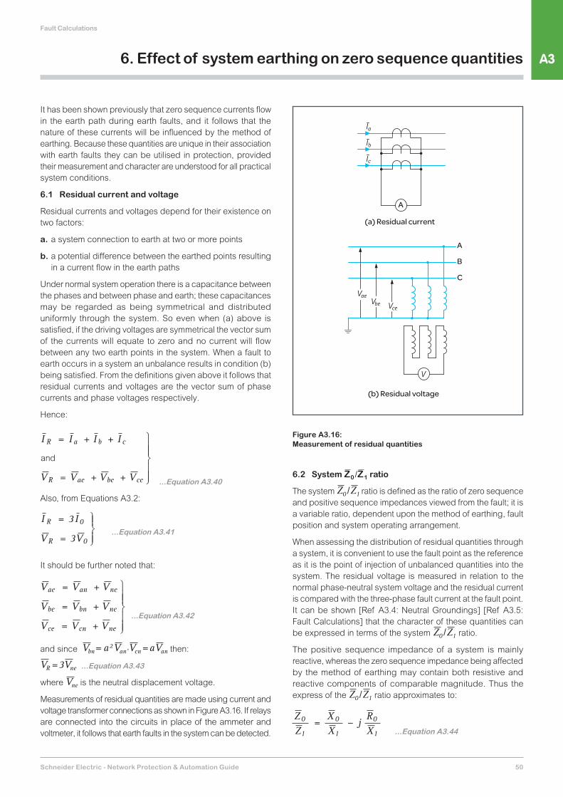
It should be further noted that:

V V V

V V V

V V V

ae an ne

be bn ne

ce cn ne

= +

= +

= +

...Equation A3.42

and since V = =bn Van'Vcn2a Vana then:

V =R Vne3 ...Equation A3.43

where Vne is the neutral displacement voltage.

Measurements of residual quantities are made using current and voltage transformer connections as shown in Figure A3.16. If relays are connected into the circuits in place of the ammeter and voltmeter, it follows that earth faults in the system can be detected.

6.2 System Z0 Z1 ratio

The system Z0 Z1 ratio is defined as the ratio of zero sequence and positive sequence impedances viewed from the fault; it is a variable ratio, dependent upon the method of earthing, fault position and system operating arrangement.

When assessing the distribution of residual quantities through a system, it is convenient to use the fault point as the reference as it is the point of injection of unbalanced quantities into the system. The residual voltage is measured in relation to the normal phase-neutral system voltage and the residual current is compared with the three-phase fault current at the fault point. It can be shown [Ref A3.4: Neutral Groundings] [Ref A3.5: Fault Calculations] that the character of these quantities can be expressed in terms of the system Z0 Z1 ratio.

The positive sequence impedance of a system is mainly reactive, whereas the zero sequence impedance being affected by the method of earthing may contain both resistive and reactive components of comparable magnitude. Thus the express of the Z0 Z1 ratio approximates to:

ZZ

XX

jRX

0

1

0

1

0

1= −

...Equation A3.44

(a) Residual current

A

C

B

A

(b) Residual voltage

Figure A3.16:Measurement of residual quantities

A3


Fault Calculations


Expressing the residual current in terms of the three-phase current and Z0 Z1 ratio:

a. Single-phase-earth (A-E)

where ZK= 0 Z1

I VZ Z K

VZ

R =+

=+( )

32

3

21 0 1

I V

Z3

1φ =

Thus:

II K

R

3

3

2φ=

+( ) ...Equation A3.45

b. Phase-phase-earth (B-C-E)

I IZ

Z ZIR = = −

+3

30

1

1 01

IV Z Z

Z Z Z1

1 0

1 0 122

=+( )+

Hence:

IV Z

Z Z Z K

VZ

R = −+

= −+( )

3

2

3

2 11

1 0 12

1

Therefore:

II K

R

3

32 1φ

= −+( ) ...Equation A3.46

Similarly, the residual voltages are found by multiplying Equations A3.45 and A3.46 by K- V .

a. Single-phase-each (A-E)

V K

KVR = −

+( )3

2 ...Equation A3.47

b. Phase-phase-earth (B-C-E)

V K

KVR =

+( )3

2 1 ...Equation A3.48

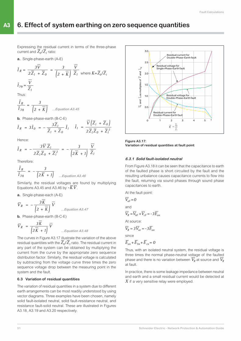
The curves in Figure A3.17 illustrate the variation of the above residual quantities with the Z0 Z1 ratio. The residual current in any part of the system can be obtained by multiplying the current from the curve by the appropriate zero sequence distribution factor. Similarly, the residual voltage is calculated by subtracting from the voltage curve three times the zero sequence voltage drop between the measuring point in the system and the fault.

6.3 Variation of residual quantities

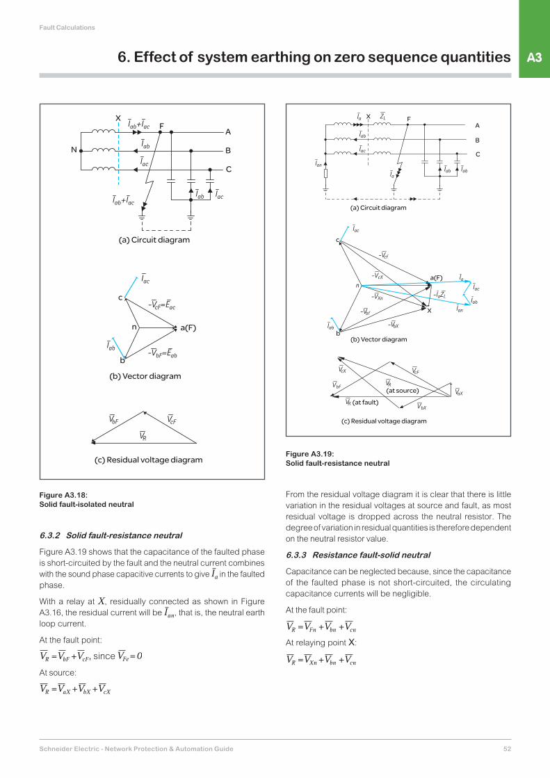
The variation of residual quantities in a system due to different earth arrangements can be most readily understood by using vector diagrams. Three examples have been chosen, namely solid fault-isolated neutral, solid fault-resistance neutral, and resistance fault-solid neutral. These are illustrated in Figures A3.18, A3.19 and A3.20 respectively.

6.3.1 Solid fault-isolated neutral

From Figure A3.18 it can be seen that the capacitance to earth of the faulted phase is short circuited by the fault and the resulting unbalance causes capacitance currents to flow into the fault, returning via sound phases through sound phase capacitances to earth.

At the fault point:

V =0aF

and

VV = + =-3R bF VcF Ean

At source:

V V= =3 -3neR Ean

since

+ = 0Ean Ebn+Ecn

Thus, with an isolated neutral system, the residual voltage is three times the normal phase-neutral voltage of the faulted phase and there is no variation between VR at source and VR at fault.

In practice, there is some leakage impedance between neutral and earth and a small residual current would be detected at X if a very sensitive relay were employed.

Residual voltage forSingle-Phase-Earth fault

Residual current forDouble-Phase-Earth fault

1 2 3 4 5 •

0.5

0

1.0

1.5

2.0

2.5

3.0

=

Residual voltage forDouble-Phase-Earth fault

Residual current forDouble-Phase-Earth fault

an

d

as m

ultip

les o

f

and

Figure A3.17:Variation of residual quantities at fault point

A3


Fault Calculations


6.3.2 Solid fault-resistance neutral

Figure A3.19 shows that the capacitance of the faulted phase is short-circuited by the fault and the neutral current combines with the sound phase capacitive currents to give Ia in the faulted phase.

With a relay at X, residually connected as shown in Figure A3.16, the residual current will be Ian, that is, the neutral earth loop current.

At the fault point:

VVV = +R bF cF, since 0V =Fe

At source:

VVV = +R aX bX V+ cX

From the residual voltage diagram it is clear that there is little variation in the residual voltages at source and fault, as most residual voltage is dropped across the neutral resistor. The degree of variation in residual quantities is therefore dependent on the neutral resistor value.

6.3.3 Resistance fault-solid neutral

Capacitance can be neglected because, since the capacitance of the faulted phase is not short-circuited, the circulating capacitance currents will be negligible.

At the fault point:

VVV = +R Fn bn V+ cn

At relaying point X:

VVV = +R Xn bn V+ cn

b

c

a(F)

X

(b) Vector diagram

(c) Residual voltage diagram

(a) Circuit diagram

C

B

AX F

(at source)

(at fault)

Figure A3.19:Solid fault-resistance neutral

(a) Circuit diagram

C

B

A

(c) Residual voltage diagram

X

N

F

b

n

c

a(F)

(b) Vector diagram

Figure A3.18:Solid fault-isolated neutral

A3


Fault Calculations

From the residual voltage diagrams shown in Figure A3.20, it is apparent that the residual voltage is greatest at the fault and reduces towards the source. If the fault resistance approaches zero, that is, the fault becomes solid, then VFn approaches zero and the voltage drops in ZS and ZL become greater. The ultimate value of VFn will depend on the effectiveness of the earthing, and this is a function of the system Z0 Z1 ratio.


(a) Circuit diagram

CBA

X

b

n

c

a

X

(b) Vector diagram

(c) Residual voltage at fault

F

F

(d) Residual voltage at relaying point

Figure A3.20:Resistance fault-solid neutral

A3


Fault Calculations

[A3.1] Circuit Analysis of A.C. Power Systems, Volume I. Edith Clarke. John Wiley & Sons.

[A3.2] Method of Symmetrical Co-ordinates Applied to the Solution of Polyphase Networks. C.L. Fortescue. Trans. A.I.E.E.,Vol. 37, Part II, 1918, pp 1027-40

[A3.3] Power System Analysis. J.R. Mortlock and M.W. Humphrey Davies. Chapman and Hall.

[A3.4] Neutral Groundings. R Willheim and M. Waters, Elsevier.

[A3.5] Fault Calculations. F.H.W. Lackey, Oliver & Boyd.

7. References

a3 · chapter 38 a3 1. introduction 39 2. three phase fault calculations 39 3. symmetrical...

Documents