aaea paper
DESCRIPTION
fsfTRANSCRIPT
7/17/2019 Aaea Paper
http://slidepdf.com/reader/full/aaea-paper 1/30
MEASURING THE EFFECTS OF GENERIC PRICE AND NON-PRICE PROMOTIONAL
ACTIVITIES: THE CASE OF WASHINGTON APPLES
Hilde van Voorthuizen, Tom Schotzko, and Ron Mittelhammer *
ABSTRACT
This paper develops a monthly domestic demand and supply equilibrium model for Washington
apples that can be used to assess the effectiveness of price and non-price promotional activities. The
econometric methodology employed takes into account market differences across the U.S. and is based on
data pertaining to individual retail stores located throughout the U.S. The period of analysis is from
September 1990 through August 2000 on a regional basis.
A unique feature of the model is its explicit allowance for multiplier effects to exist between the
level of print media (newspaper ad and flyers) expenditures provided by the Washington State Apple
Commission (WAC) in support of apple demand and supplementary funds provided by retailers in
support of apple promotion.
In particular the model allows for the fact that Commission funds oftentimes represent only a
relatively small fraction of the overall print media expenditures made in support of apple sales, and that
Commission funds are often effectively only “pump priming” or serve as inducements for additional
promotional activities by other entrepreneurs in the marketing chain. Also, the subset of promotional
activities (print media and price reductions) provided by retailers is modeled in a dynamic fashion,
whereby market conditions feedback affects the level of apple promotion provided by retailers.
The overall model includes a set of retail demand equations, a set of retail-F.O.B. price linkage
equations, a set of ad lines – WAC Ad buys linkage equations, and an aggregate industry supply function.
Additional factors such as asymmetry in retail-F.O.B. price response, the effects of information
technology in retail pricing, and the effects of the large crops and the Asian and the Mexican crises on
domestic supply are all simultaneously considered.
Results of this analysis indicate that, in the aggregate, price promotion is a significant factor
positively impacting apple sales. Furthermore, price promotion elasticities were relatively high when
compared to non-price promotional activities, leading to a conclusion that greater gains with respect to
returns on promotional investment may occur when retail price reductions are pursued.
* Hilde van Voorthuizen is Assistant Professor, California Polytechnic State University. Tom Schotzko is
Extension Economist, and Ron Mittelhammer is Professor in the Departments of Agricultural Economics
and Statistics, Washington State University

7/17/2019 Aaea Paper
http://slidepdf.com/reader/full/aaea-paper 2/30
2
Despite an increased domestic supply and the effects of the Mexican and the Asian crises, among
the non-price promotional activities, results indicated that both non-trade (TV and Radio) and trade-
related efforts (in store demonstrations, point of sale displays, promotional give-aways, and ad buys) have
contributed to increased demand for Washington apples. Sensitivity analysis of trade and non-trade
expenditures indicated that trade-related activities were more effective in increasing demand at current
expenditure levels relative to non-trade activities. Promotional efforts in the form of billboards, food
service expenditures, and other miscellaneous activities, which the industry also carried out during the
historical period of analysis, did not have a measurable impact on demand in any of the regions.
It was also found that WAC ad buy expenditures resulted in a multiplier effect on the total
number of ad lines. While the direct effect of these Commission expenditures on demand would be
relatively small without the supplementary efforts forthcoming from retailers, the fact that retailers
multiplied the Commission’s expenditures into a substantially larger promotional effort resulted in a
significant positive effect on apple sales when viewing the promotion program as a whole.
Key words: price and non price promotion, trade and non trade activities
7/17/2019 Aaea Paper
http://slidepdf.com/reader/full/aaea-paper 3/30
3
MEASURING THE EFFECTS OF GENERIC PRICE AND NON-PRICE PROMOTIONAL
ACTIVITIES: THE CASE OF WASHINGTON APPLES
1. Introduction
Commodity programs and retailers in joint agreement or as separate entities, often conduct
broadcast media and/or sales promotion to acquaint, or remind, consumers about the attributes of the
products they have to offer. Cents-off, in store demonstrations, and point-of-purchase displays are types
of sales promotion devices designed to supplement advertising and, sometimes, personal selling in the
promotional mix (Cateora and Graham). The apple industry in the state of Washington has a long
tradition in implementing most of these strategies through the Washington Apple Commission, which is
an institution created by the industry to coordinate marketing efforts for long-term profitability.
Specifically, the Commission conducts non-trade promotional activities (TV and Radio) and trade-related
activities (ad-buy/print media, product display, and other trade merchandising activities). Within the print
media category, however, Commission funds often represent only a relatively small fraction of the overall
print media expenditures made in support of apple sales. The Commission funds are often effectively only
“pump priming” or serve as inducements for additional promotional activities by other entrepreneurs in
the marketing chain.
While several studies of commodity promotion evaluation have established a precedent for
analyzing promotion and advertising’s performance through models of demand response, (Richards and
Patterson, Chung and Kaiser, Capps and Moen, Kinnucan and Miao to mention a few), these studies have
not considered the multiplier effect that may result from joint agreements in sales promotion.
This paper develops a monthly domestic demand and supply equilibrium model for Washington
apples that can be used to assess the effectiveness of price and non-price promotional activities, while
considering the multiplier effects of joint sales promotion agreements. This paper presents a synthesis of
economic theory as well as institutional realities, practical experience and knowledge gleaned from
industry sources upon which each model component is based. Major findings pertaining to the demand,
supply, print media multiplier effect, and industry returns per promotion type are also reported.
2. Methodology
The econometric methodology takes into account market differences across the U.S. and is based
on data pertaining to individual retail stores located throughout the U.S.1 The overall model includes a set
of retail demand equations, a set of retail-F.O.B. price linkage equations, a set of ad lines – WAC Ad buys
linkage equations, and an aggregate industry supply function, the former three differentiated by regions of
the U.S. In addition, factors such as asymmetry in retail-F.O.B. price response, the effects of information
technology in retail pricing, and the effects of the large crops and the Asian and the Mexican crises on
7/17/2019 Aaea Paper
http://slidepdf.com/reader/full/aaea-paper 4/30
4
domestic supply are all simultaneously considered in the evaluation process. Data sources are shown in
Appendix Table 1. Each model component is defined as follows:
2.1 The Demand Model
The demand for Washington apples is specified on a regional and a per capita basis and is a
function of a vector of prices, income, price and non-price promotional expenditures, and other variables
having an influence or demand. Thus, the demand function is empirically approximated as follows:
(1) QDW tr /POP tr = f (P retail t *(1-adexptr ) , Adpricetr *adexptr , RINC tr / POP tr , PP t ,, ,
0
n
i=∑ Adlinest-i,r ,
0
n
i=∑ ADV t-i,j,r /POP t-i, r j∀ , QDW t-1,r /POP t-1,r ,
QDWRt-12,r /POP t-12 ,r , t T ,2
t T ,3
t T , 0
n
i=∑ Logost-i,,r ,0
n
i=∑ Color t-i,r , , t ,
4
1
Region other, ur tr
r
,=
∑
Where:
retailer
QDW total quantity demanded of apples in month , region ;
Pop population in month , region (expressed in millions);
P the regular retail price per pound of Washington apples that prevtr
t
tr
t r
t r
≡
≡
≡ ailed during
month , region ;Adprice the promotional retail price per pound of Washington apples that prevailed
during month , region ;
Adexp the time an ad is in effect in a given month expres
tr
tr
t r
t r
≡
≡ sed in ratio form;
RINC the real disposable personal income per million people in month , region ;
PP a vector of substitutes measured in price per pound in month , specifically
bananas, and pears
tr
t
t r
t
≡
≡
-
;
ADV a vector of advertising expenditures per million people in period - , for
0, 1, ,n; in category , region . For mass media, trade merchandising
(display, give away products, trade se
t ijr t i
i j r j
≡
= =…
rvices, and other in-store promotional
activities);
Adlines the weighted number of ad lines in month , region ;
Color the weighted number of lines in a colored format in month , region ;
tr
tr
t r
t r
≡
≡
7/17/2019 Aaea Paper
http://slidepdf.com/reader/full/aaea-paper 5/30
5
1
12
Logos the weighted number of ads containing a logo in month , region ;
QDW total quantity demanded of apples in month , region , lagged one period;
QDW total quantity demanded of apples
tr
t ,r
t ,r
t r
t r −
−
≡
≡
≡
2 3
in month , region , lagged 12 periods;
a polynomial time trend to capture seasonal consumption patterns, where
1 12
Other Other variables having an impact on
t t t
t t
t r
T ,T ,T
T in January, ...,T in December;
≡
= =
≡ demand such as quantities of apples
demanded from New York, Michigan, and California, a time trend capturing
secular changes in demand.
the error term to capture any remaining effect not included intr u ≡ the model.
In equation (1), all prices and advertising expenditures are in real terms. Details can be found in
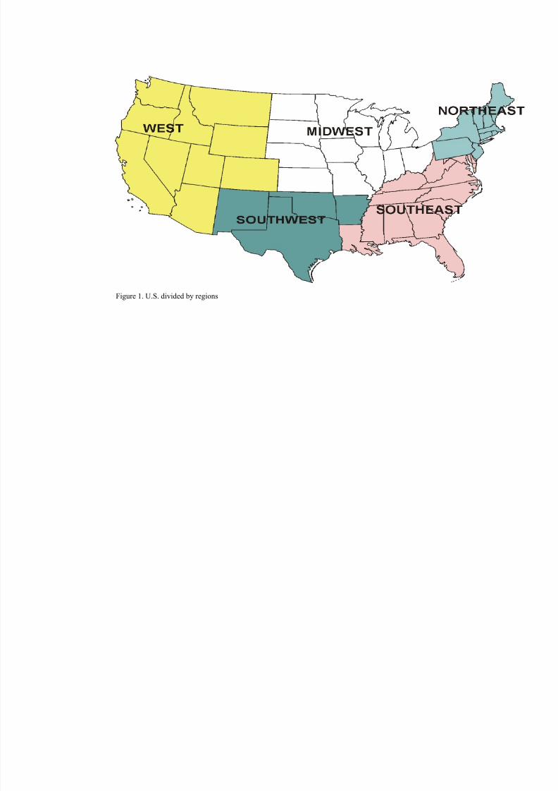
Van Voorthuizen. The regions are chosen based on territorial sales and population distributions as
specified in Figure 1. The selection of the regional boundaries is influenced by information received
regarding W.A.C. field representative territories. Note that regions are introduced in the model through
indicator variables2. The Southwest indicator variable is excluded from the model and the Southwest
becomes the base region for the analysis.
Important characteristics of the demand equation specification to note include: 1) the regular
retail price and the promotional price are adjusted by a variable that accounts for the amount of time each
price was in effect in a regional market, 2) the seasonal effects are captured by a polynomial time trend
based on observed shipment patterns throughout the marketing season (t, t2, and t3), 3) physical measures
of printed ads are used instead of expenditures (ad lines, ad containing a logo and colored ads); and 4)
advertising carryover effects are evaluated using two lagged variables 1 12andt- ,r t - ,r QDW QDW . The
procedure used to capture the advertising and promotion carryover effects is different from procedures
suggested by Nerlove and Waugh, Carman et al. Chung and Kaiser.
In the final model the variables proxying persistent consumption behavior,
( )1 12andt - ,r t- ,r QDW QDW , prove to be statistically significant. Equation (2) depicts the cumulated carry
over effect through time.
(2) ( QD∂ / Adv∂ )12months.cum = QD∂ / t , j Adv∂ + ∑=
11
1i
( QD∂ / it QD −∂
* it QD −∂ / 1it QD −−∂ * 1it QD −−∂ / 1it , j Adv −−∂ ) = advj β + ∑=
11
1i
jit advQDi * β β −

7/17/2019 Aaea Paper
http://slidepdf.com/reader/full/aaea-paper 6/30
6
In Equation (2), QD represents QDW/POP for simplicity of notation. Also, Adv j is defined as Adv j /POP
(advertising expenditure per million people for category j). The β ’s are the corresponding estimated
coefficients, i = 1 (past month), 2,…,11th past month in which advertising expenses occurred, but still
positively impacting the current month’s consumption. Similarly, the marginal cumulative advertising
effect on demand in the 13th month holding other variables in the entire system constant is given by:
(3) ( QD∂ / j Adv∂ )13months, cum = QD∂ / t Adv∂ + ∑=
12
1i
( QD∂ / it QD −∂ * it QD −∂ / 1it QD −−∂ *
1it QD −−∂ / 1it , j Adv −−∂ ) + ( QD∂ / 1t QD −∂ * 1t QD −∂ / 13t QD −∂ * 13t QD −∂ / 13t , j Adv −∂
+ QD∂ / year st 1 ,12t QD −−∂ * year st 1 ,12t QD −−∂ / / QD*QD 13t 13t −− ∂∂ 13t , j Adv −∂ )
In Equation (3), the advertising carry-over effects in the thirteenth-month can be added to the cumulated
carryover effects of the first marketing year. Cumulated advertising carryover effects for subsequent periods are obtained by continuing to differentiate the above equation through time and continuing to
accumulate the results.
2.2 Adlines Response
In terms of print media (newspaper ads), the Commission partially covers the cost of apple ads in
print media used by retailers. These expenditures are not included in the demand model because
considerably more information regarding size of ad as well as ad attributes (logos, color and illustrations)
is available and was used to refine the analysis of the effects of this type of promotion activity. The sizeof print ad is measured in terms of the number of lines appearing in an ad as measured in standard
newspaper lineage (ad lines).
To determine the impact of ad buys on retail demand and, later, on derived benefit-cost ratios, an
ad line-ad buy linkage equation (4) is formulated and estimated:
(4) Adlinestr = +o β 1 2 1 3 12 4 1Pretailtr tr tr tr Adbuys Adlines Adlines β β β β − − −+ + + +
11
5
1
i i
i
B Season
=
∑
where : i β are parameters to estimate, for i = 0, 1, 2…,5;

7/17/2019 Aaea Paper
http://slidepdf.com/reader/full/aaea-paper 7/30
7
1
Adlines the weighted number of ad lines appearing in month , region ;
Adbuys the total amount of ad buy expenditures authorized by WAC in month ,
region , expressed in real terms;
Adlines th
tr
tr
tr-
t r
t
r
≡
≡
≡
12
e weighted number of ad lines lagged one period;
Adlines the weighted number of ad lines lagged twelve periods;tr - ≡
1Pretail the regular retail price lagged one period and expressed in real terms in
month , region ;
Season January, February, , December indicator variables to account for seasonal
effects.
tr-
i
t r
≡
≡ …
Equation (4) is needed because retailers do some level of newspaper advertising beyond the
advertising supported by Commission funding. However, the ratio of the Commission supported ads to
total ads is unknown.
In Equation (4), ad buys are expected to have a positive effect on the number of weighted ad lines
in period t. Also, it is hypothesized that the number of ad lines in a specific period would depend on how
much advertising is conducted in the previous month and one year earlier. Therefore, ad lines lagged one
period and ad lines lagged 12 periods were both included in the model and are expected to have positive
impacts on current ad lines.
Regional retail prices are also included in the lines equation so as to examine the effect of retailer
participation in response to changing retail prices. It is hypothesized that when regular retail prices
decrease, retailers advertise more. Equation (4) is specified on a regional basis to account for any regional
differences in the number of ad lines placed during the year. Also, it is hypothesized that the industry
would tend to advertise more in the fall and winter months relative to spring and summer for two reasons:
the new crop becomes available in the fall, and because of the Christmas holidays. September is the base
period for seasonality.
2.3 The Supply and Price Transmission Models
During the period of study (September 1990 through August 2000), the Washington Apple
industry was exposed to factors that exerted a direct impact on supply response. Among those factors are
seasonal effects, the Mexican devaluation, Asian economic crisis, and inventory levels, to mention a few.
Each factor was thought to impact month-to-month decisions in terms of product allocation in domestic
markets. Hence, the supply of Washington apples is empirically modeled as:
7/17/2019 Aaea Paper
http://slidepdf.com/reader/full/aaea-paper 8/30
8
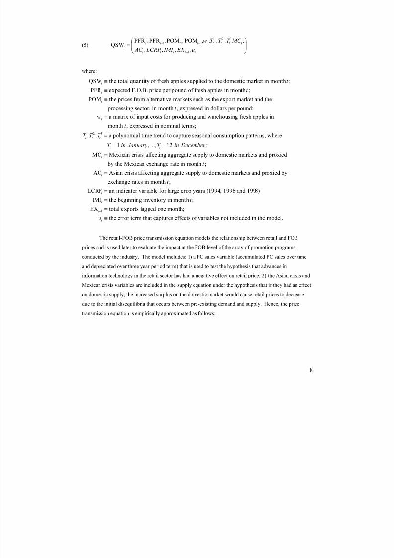
(5)
2 3
1 1
1
PFR PFR POM , POM , ,QSW t t- t t- t t t t t
t
t t t t t
, , w T ,T ,T MC ,
AC ,LCRP ,IMI ,EX ,u−
=
where:
QSW the total quantity of fresh apples supplied to the domestic market in month ;
PFR expected F.O.B. price per pound of fresh apples in month ;
POM the prices from alternative markets such as the
t
t
t
t
t
≡
≡
≡
2
export market and the
processing sector, in month , expressed in dollars per pound;
w a matrix of input costs for producing and warehousing fresh apples in
month , expressed in nominal terms;
t
t t
t
t
T ,T
≡
3 a polynomial time trend to capture seasonal consumption patterns, where
1 12
MC Mexican crisis affecting aggregate supply to domestic markets and proxied
by the Mexica
t
t t
t
,T
T in January, ...,T in December;
≡
= =
≡
n exchange rate in month ;
AC Asian crisis affecting aggregate supply to domestic markets and proxied by
exchange rates in month ;
LCRP an indicator variable for large crop years (1994, 1996 and 199
t
t
t
t
≡
≡
1
8)
IMI the beginning inventory in month ;
EX total exports lagged one month;
the error term that captures effects of variables not included in the model.
t
t
t
t
u
−
≡
≡
≡
The retail-FOB price transmission equation models the relationship between retail and FOB
prices and is used later to evaluate the impact at the FOB level of the array of promotion programs
conducted by the industry. The model includes: 1) a PC sales variable (accumulated PC sales over time
and depreciated over three year period term) that is used to test the hypothesis that advances in
information technology in the retail sector has had a negative effect on retail price; 2) the Asian crisis and
Mexican crisis variables are included in the supply equation under the hypothesis that if they had an effect
on domestic supply, the increased surplus on the domestic market would cause retail prices to decrease
due to the initial disequilibria that occurs between pre-existing demand and supply. Hence, the price
transmission equation is empirically approximated as follows:

7/17/2019 Aaea Paper
http://slidepdf.com/reader/full/aaea-paper 9/30
9
(6) Pretail tr = α + ∑=
5
1r
b1r (RI r * Pretail t-,1,r
)+ ∑=
5
1r
b21r (RI r *PFI t )+
∑=
5
1r
b22r (RI r *PFF t )+ ∑=
5
1r
b3r (RI r *TC t )+ ∑=
5
1r
b4r (RI r *Waget + ∑=
5
1r
b5r (RI r *PCsalest ) +
b6 *MC t + B7 *AC t + ∑11
i
b8 Seasonalityi
Where:
8765322211 b ,b ,b ,bj ,..b ,b ,b ,b , j j j jα estimated parameters,
Pretail the nominal retail price per pound of Washington apples in region ,
month , expressed in nominal terms;
RI regional indicator variables, 1 2 5. Where 1 is for the Midwest, 2 for
the No
tr
r
r
t
j , , ,
≡
≡ = …
1
rtheast, 3 for the Southeast, 4 and 5 for the Southwest and West,respectively;
Pretail the nominal lagged retail price per pound of Washington apples in region ;
PFI a vector of cumulative increa
t - ,r
t
r ≡
≡ ses in the nominal F.O.B. price per pound of
fresh apples in month ;
PFF a vector of cumulative decreases in the F.O.B. price per pound of fresh
apples in month and expressed in nominal terms
TC a
t
t
t
t
≡
≡ U.S. transportation cost index in month ;
Wage a U.S. retail wage index in month ;MC a variable to capture the Mexican crisis effects and is proxied by the
exchange rate in month ;
AC a variable
t
t
t
t
t
t
≡≡
≡ to capture the Asian crisis effects and is proxied by a weighted
exchange rate in month ;
PCsales the total nominal value of cumulated and depreciated personal computer
sales in the U.S. in month ;
S
t
t
t
≡
easonality indicator variables for each month of the year, where 1 is for January, ,
and 12 is for December.
≡ …
In the above model, retail price stickiness is tested through the lag of the dependent variable.
Asymmetry in retail price response with respect to FOB price changes is examined through the method
suggested by Kinnucan and Forker.
7/17/2019 Aaea Paper
http://slidepdf.com/reader/full/aaea-paper 10/30
10
2.4 Average Industry Returns
Once the supply, demand, ad line-ad buy, and price transmission relationships were estimated,
each month’s equilibrium conditions and other endogenous variables in the system (e.g., ad lines and
retail prices) were solved simultaneously. The exogenous variables were evaluated at their historical
monthly levels except for those variables that were directly affected by the endogenous variables (e.g.
shipments and inventories), which also were solved simultaneously. The monthly results were then used
to solve the next month’s results in an interactive fashion. Once the equilibrium was determined for the
entire period of analysis, revenues with advertising and revenues under simulated scenarios of no
advertising were computed and summed across months within a year. The differences in annual revenues
with and without advertising were then divided by the annual difference in the cost of the advertising
programs. The outcome is a benefit-cost ratio, which is used as the basis for determining average
industry returns to advertising and promotion.
3. Results
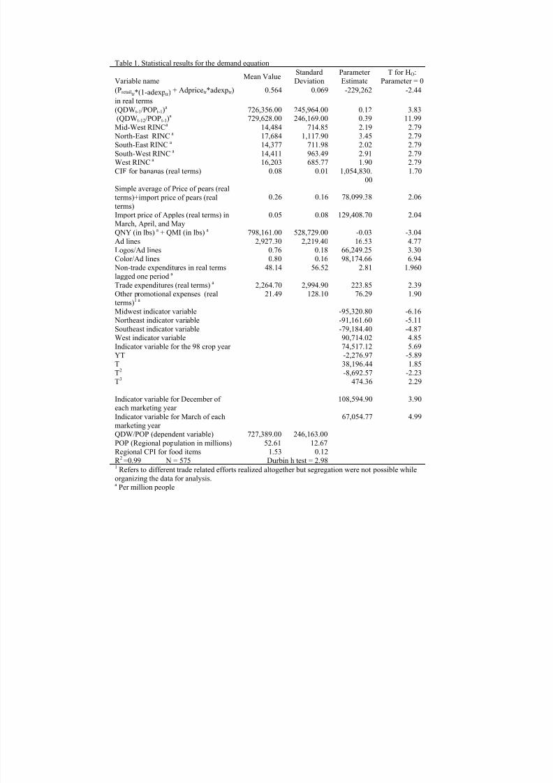
3.1 Demand Model
Except for the polynomial time trend used to capture seasonal patterns in consumption, the final
demand model was linear in all of the variables and in their respective parameter estimates. The model
was estimated using 2SLS. The endogenous variables in the final model were total quantity shipped of the
five varieties (Red and Golden Delicious, Granny Smith, Gala, and Fuji), retail price, promotional price of
Washington apples, the current month’s trade category expenses, and the current month’s ad lines. The R 2
for the second stage is reported in Table 1. The Durbin h test reported in Table 2 suggests that no
autocorrelation is present. Descriptive statistics and coefficient estimates from the second stage of 2SLS
are also reported in Table 1.
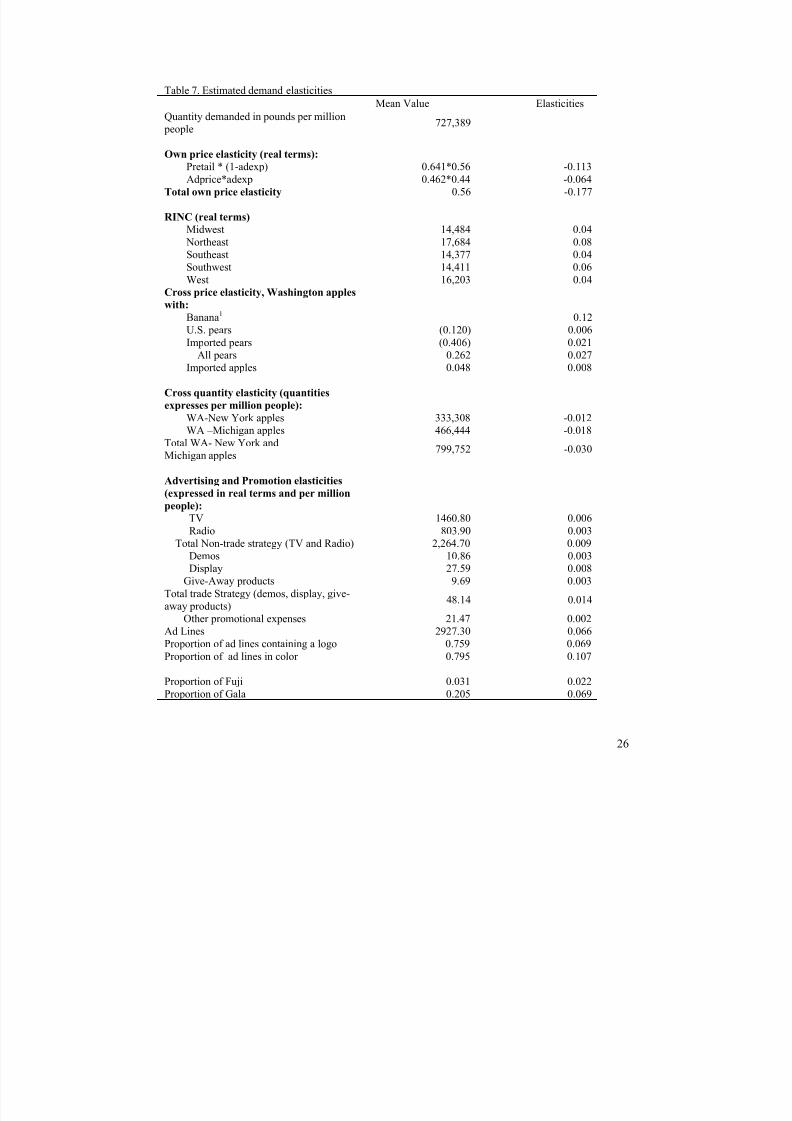
3.1.1 Price Promotion Effects
The retail price and the promotional price coefficients were found through a Wald test to be
insignificantly different. Therefore, a single weighted measure of the form ( P retail tr *(1-adexptr ) +
Adpricetr *adexptr ) was created to replace the individual variables in the final demand equation. The
weighted price is expressed as price per pound in real terms. The mean value of the new weighted price
per pound is 0.564 cents. The marginal effects of either type of price change are the same, suggesting that
a dollar increase (a dollar decrease) in either price, in a given region, would decrease (increase) monthly
regional demand by the value of 229,262 pounds per million people3
The retail price elasticity is -0.113 percent while the corresponding promotional price elasticity is –0.06
percent (Table 7).
7/17/2019 Aaea Paper
http://slidepdf.com/reader/full/aaea-paper 11/30
11
3.1.2. Effects of Non-Price Promotional Efforts
Based on the outcome of a Wald test, demos, displays, and giveaway products were aggregated
into one category (trade category). Similarly, radio and TV were aggregated into a single category (non-
trade category) according to the results of the Wald test. Both categories had significant and positive
impacts on the demand for Washington apples. Table 7 shows the corresponding elasticities.
Other promotional expenditures such as food service, trade, billboards, and Run on Press (these
are the ads produced directly by W.A.C. and supplied to retailers) did not have individual statistically
measurable impacts on the demand for Washington apples. Thus, these variables were removed from the
final model. Ad lines had a positive effect on regional demand.
Regarding logos and color ads (Table 1), throughout the estimation process, expressing the
demand equation as a function of total number of logos and total color ad lines created multicollinearity
problems, hence, the proportion of logos and the proportion of color ads were used and had positive and
significant additive effects on the demand for Washington Apples.
Lag structures were also tested throughout the modeling process. Only the non-trade strategy
category lagged one-month was significant. The lags of the other promotional activities were non-
significant.
3.1.3 Persistent Preferences and Promotional Effects
Cumulative promotion effects on current demand were induced by persistent preferences (Table
1). The previous month’s consumption of apples was positively related to the current month’s
consumption. Also, apple consumption in the corresponding month of the previous year was also
positively related to the consumption of apples in the current month. The significance of the lagged
quantity variables (quantity lagged one period and quantity lagged twelve months) implies that additional
returns accrue to promotion activities in the long run as compared to the short run.
3.1.4 Other Factors Affecting Demand
The regional income variables (RINC) in Table 1 were highly correlated amongst each other.
Principal component analysis was used to mitigate the multicollinearity problem. The income variable
coefficients associated with the principal component scores were positive and significant across regions
indicating that apples are normal goods and as income rises, a greater quantity of apples is demanded.
Note that the t-values across regions are the same because only one principal component was used to
represent the collinear income variables.
7/17/2019 Aaea Paper
http://slidepdf.com/reader/full/aaea-paper 12/30
12
Substitutes in the final demand model (Table 1) were imported apples, Michigan and New York
apples, imported and domestic pears, and imported bananas. The Wald test indicated that the effects of
Michigan and New York shipments were insignificantly different, and these variables were combined in
the final model. An increase (decrease) in Michigan and/or New York shipments reduces (increases)
demand for Washington apples.
The imported apple price effects were measured in interaction with March, April, and May,
which are the months when imports are most pronounced and when domestic shipments of Washington
apples are higher relative to the rest of the season. Import price interacted with the months of June and
July were also tested, but the effect was non-significant. The coefficient sign for the imported apple price
interacting with March, April, and May was positive as hypothesized. The magnitude of estimate was
129,408.70 indicating that as price increases (decreases) by a dollar, demand for apples would increase
(decrease) by 129,408.70 pounds.
Imported and domestic pear prices also had the hypothesized sign and they were significant in
magnitude. These variables were introduced in the model as the simple average of both prices. A volume
weighted measure of both prices was tested, but it was non-significant. The coefficient for the CIF price
of bananas was also significant and positive as initially hypothesized.
Seasonality of demand was also evident across months within a marketing year (Table 1). By
adding the seasonal time trend (2 3, ,t t t T T T ) and evaluating it at each month of the year (1 for January, 2
for February, ..., 12 for December), differences in demand across seasons is apparent. Differences in
consumption patterns throughout the U.S. were also detected in the final results. In addition to the
polynomial time trend, the overall yearly time trend (YT) included in the model to capture secular
changes in demand over time was also found to have a negative impact on the current month’s demand
for Washington apples. The negative coefficient for the time trend variable potentially reflects the
emergence of more diverse eating habits and the growing demand for specialty and ethnic fruits over
time.
3.2 Adlines Model
Each regional ad lines equation, as specified in (4), was estimated using OLS. This method was
used because all variables used to describe the behavior of ad lines were considered predetermined,
including ad buys. The Hausman test for endogeneity was non-significant, supporting OLS as the
appropriate regression technique. The R 2 ranged from 0.77 to 0.82 suggesting the exogenous variables in
each equation explained most of the variation in ad lines. The autocorrelation tests were insignificant for
all equations.

7/17/2019 Aaea Paper
http://slidepdf.com/reader/full/aaea-paper 13/30
13
All variables in each of the equations were expressed in linear form. The ad lines observations
contained unexplained outliers. Therefore, indicator variables for the months in which these outliers
occurred were added to the model. The anomalous outliers were not consistent across regions so the
indicator variables for the outliers vary across equations (regions). Results for each individual equation
are shown in Tables 2 through 6.
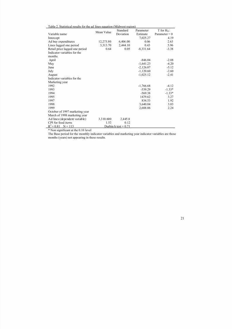
According to the results in Tables 2 through 6, specific inferences can be made with respect to the
manner in which ad lines appear in a region and their relationship with the WAC’s ad buys/print media
expenditures. These inferences are the following:
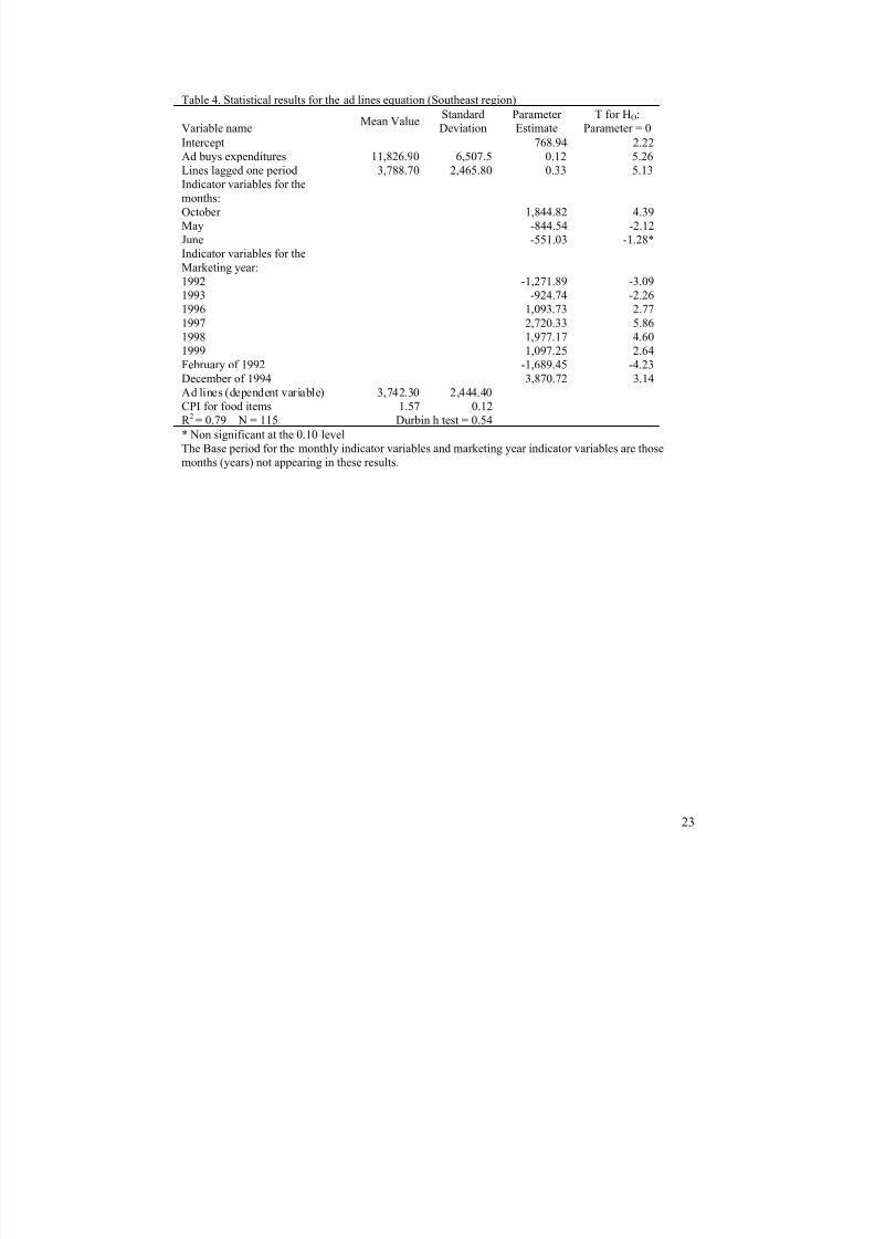
1) The coefficients of ad buys and the level of ad buy expenditures for the Midwest and
Southeast region are higher relative to the other regions. The ad lines-ad buys elasticity
evaluated at the mean level for both regions were 0.24 and 0.37, respectively.
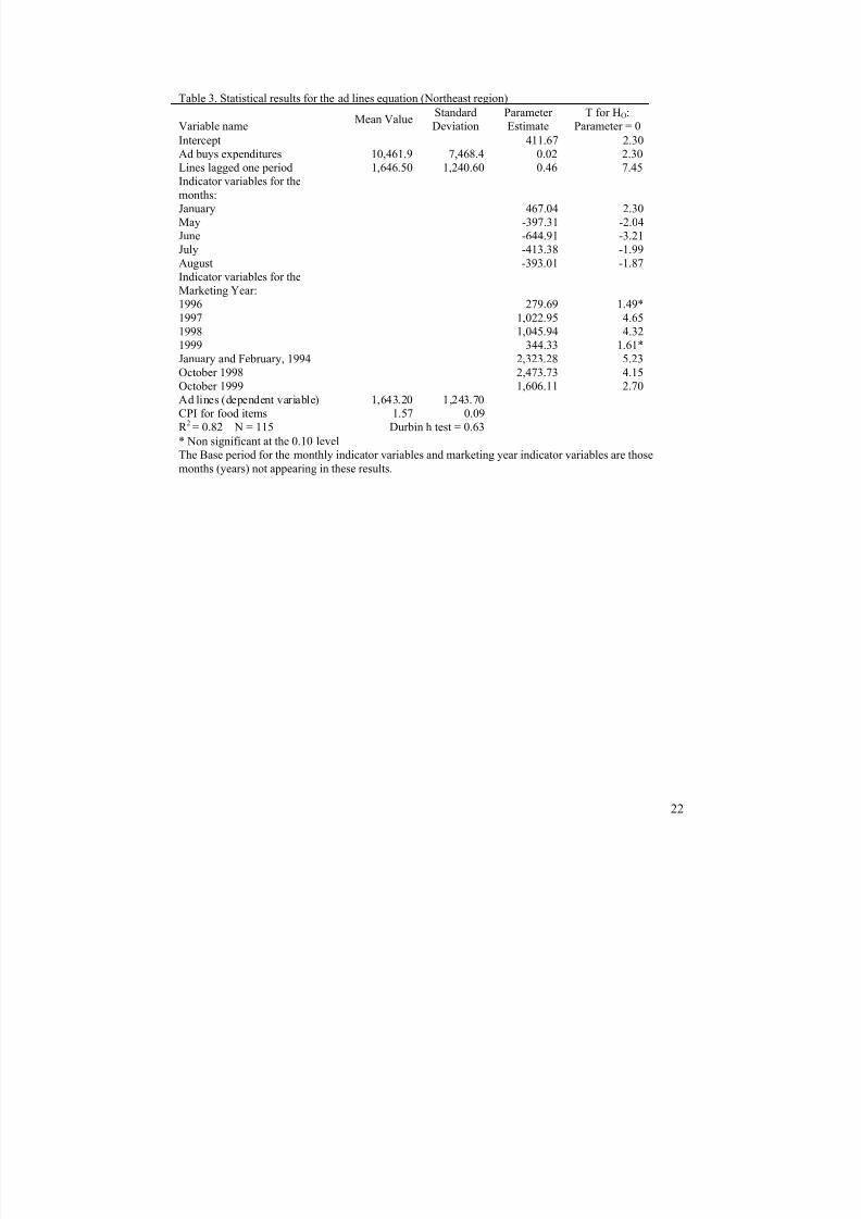
2) The ad line-ad buy elasticity evaluated at the mean level for the Northeast and West region
were 0.14 and 0.21 respectively.
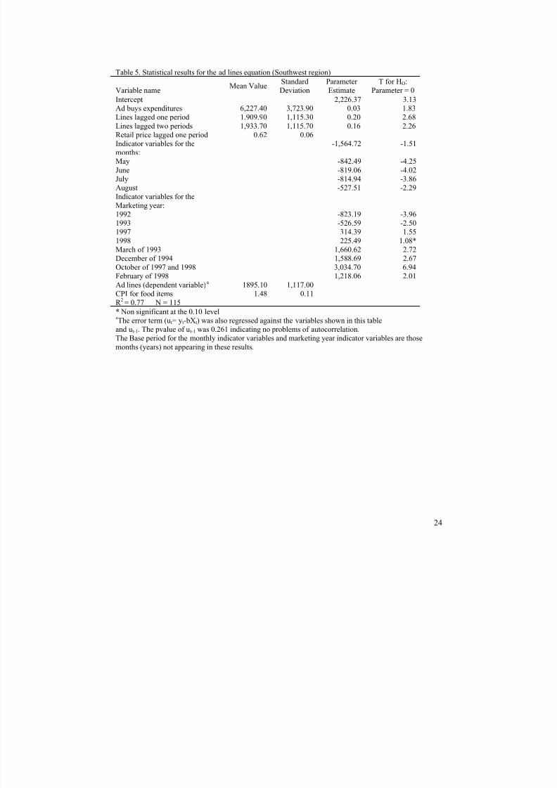
3) The Southwest region had the lowest coefficient and lowest level of ad buy expenditures
among all regions. The elasticity evaluated at the mean level was 0.10 percent.
4) These elasticities reflect the level of funding the commission contributes to overall print
media.
5) The number of ad lines used in the current period depends on the number of ad lines that
were used in the past month for all regions. Ad lines lagged 12 periods were not a significant
factor in explaining current period ad lines.
6) Fewer ad lines are run in late spring and in early summer in each marketing year in all
regions.
7) More ad lines were used in marketing years of 1997 and 1998 in all regions relative to other
marketing years.
3.3 The Supply Model and the FOB-Price Transmission Model
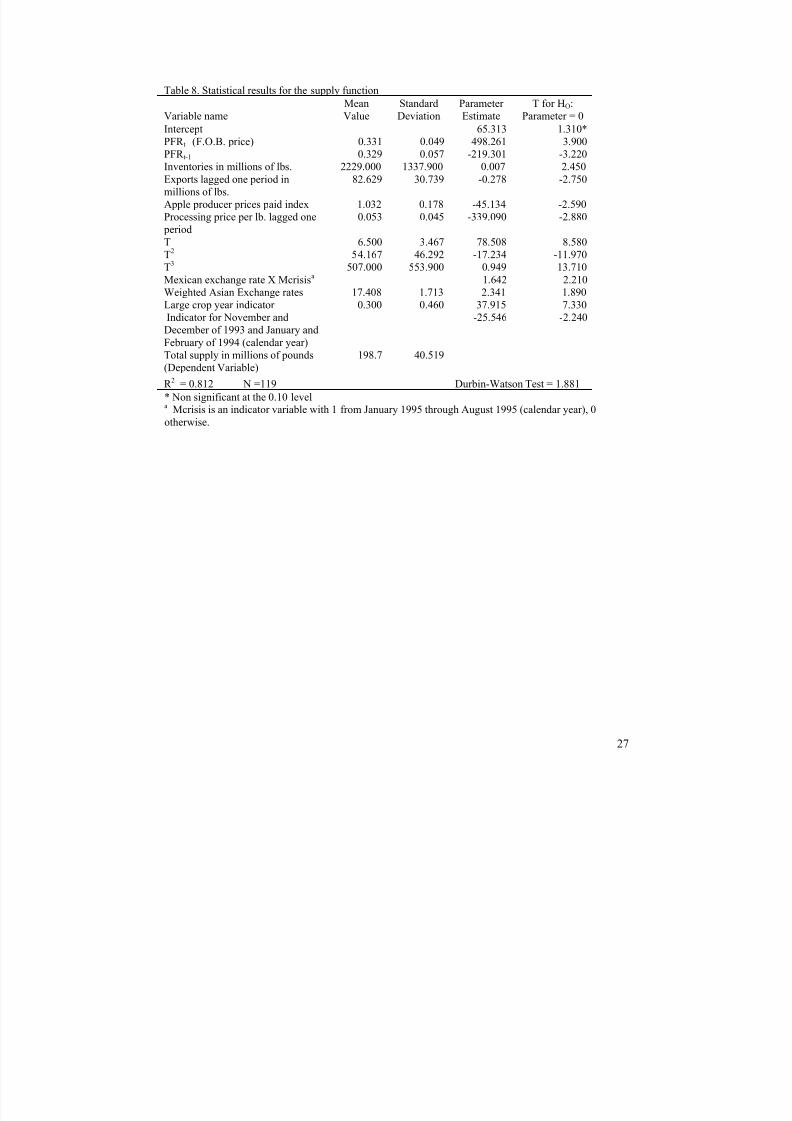
Each coefficient significance level supported our a priori hypotheses. The R 2 of the supply model
(0.810) indicated that most of the variability occurring in quantity supplied was explained by the
variability of the explanatory variables (Table 8).
Among the results for the supply equation, the most intriguing one is that the lagged FOB price
parameter estimate was negative (Table 8). However, when both the current month and past month
7/17/2019 Aaea Paper
http://slidepdf.com/reader/full/aaea-paper 14/30
14
effects are jointly analyzed1 the results make sense from the packer’s perspective. Rising F.O.B. prices
(both current and lagged) will cause an increase in the current month’s volume shipped. However, the
increase will be muted as some packers anticipate further price increase and attempt to restraint sales to
take advantage of those anticipated price increases in the future.
Conversely, a declining F.O.B. price will reduce the current month’s quantity supplied. However,
the decrease will be partially offset as some packers anticipate further declines and attempt to move
additional quantities before profits vanish.
Logically, when lagged price and current price move in opposite directions, the effect of the
current FOB price on quantity supplied is amplified by the lagged price effect. Mixed price signals may
increase packer’s uncertainty about the future causing an exaggerated response to current market
conditions.
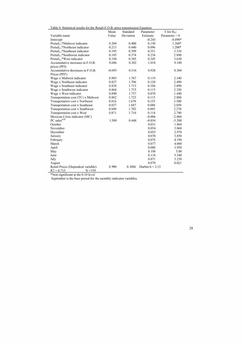
Results for the price transmission equation are shown in Table 9. Results for all variables are as
initially hypothesized. The “price stickiness” of retail prices was confirmed. Moreover, the relationship
between retail and FOB prices was found to be asymmetric, with retail price response to increases and
decreases in the FOB prices being statistically different in magnitude.
3.4 Industry Returns
Benefit cost ratios pertaining to this analysis are shown in Table 10. For all years, benefits were
greater than one indicating that for each dollar invested in advertising and promotion, the industry
received more than a dollar in increased returns. However, trade-merchandising activities, including the
ad-buys/print media multiplier, were greater relative to the non-trade activities.
4. Conclusions
This paper developed a monthly domestic demand and supply equilibrium model for Washington
apples that can be used to assess the effectiveness of price and non-price promotional activities. The
econometric methodology employed took into account market differences across the U.S. and is based on
data pertaining to individual retail stores located throughout the U.S. The period of analysis is from
September 1990 through August 2000 on a regional basis.
A unique feature of the model is its explicit allowance for multiplier effects to exist between the
level of generic advertising expenditures provided by the Washington State Apple Commission in support
of apple demand and supplementary funds provided by retailers in support of apple promotion,
specifically through print media ads.
1 The authors examined several models of supply. The final model presented in this article appeared to be the most
defensible when considering both statistical and economic implications of the results.
7/17/2019 Aaea Paper
http://slidepdf.com/reader/full/aaea-paper 15/30
15
In particular the model allows for the fact that Commission funds oftentimes represent only a
relatively small fraction of the overall print media expenditures made in support of apple sales, and that
Commission funds are often effectively only “pump priming” or serve as inducements for additional
promotional activities by other entrepreneurs in the marketing chain. Also, the subset of promotional
activities (print media and price reductions) provided by retailers is modeled in a dynamic fashion,
whereby market conditions feedback affect the level of promotion that retailers contribute in support of
apple demand.
Results of this analysis indicate that, in the aggregate, price promotion is a significant factor
positively impacting apple sales. Furthermore, price promotional elasticities were relatively high when
compared to non-price promotional activities, leading to a conclusion that greater gains with respect to
returns on promotional investment may occur when retail price reductions are pursued.
The relative importance of price promotions is particularly salient given the price stickiness
observed in this model. Reducing price at the FOB level does not result in an immediate reduction in
price at the retail level. Further, the retail price decline, when it does occur, does not reflect the full
decline that occurred at the FOB level.
It is commonly believed within the Washington industry that retailers tend to establish an
“everyday” price at the beginning of the season and maintain that price as long as it remains within some
acceptable range of competitor prices. Assuming this belief to be a reasonable reflection of reality, the
results of this model imply that a key WAC activity would be to attempt to influence the initial prices set
at retail in light of the projected crop size.
Despite an increased domestic supply and the effects of the Mexican and the Asian crises, among
the non-price promotional activities, results indicated that both non-trade (TV and Radio) and trade-
related efforts (in store demonstrations, shippers display, and products give-away, ad buy-print media
expenditures) have contributed to increased demand for Washington apples. When scenarios of varying
levels of expenditures made in each type of these specific promotional activities were examined, it was
found that the trade-related activities were more effective in increasing demand at current expenditure
levels relative to the non-trade activities. Promotional efforts in the form of billboards, food service
expenditures, and other miscellaneous activities, which the industry also used during the period of
analysis, did not have a measurable impact on demand in any of the regions.
Regarding the Commission ad buy-print media expenditure multiplier effect, it was found that the
Commission’s promotional efforts in this specific promotional outlet in fact did constitute only a
relatively small fraction of the overall print media efforts by retailers. While the direct effect of
Commission expenditures on demand would be relatively small without the supplementary efforts
forthcoming from retailers, the fact that retailers multiplied the Commission’s expenditures into a

7/17/2019 Aaea Paper
http://slidepdf.com/reader/full/aaea-paper 16/30
16
substantially larger promotional effort resulted in a substantially positive effect on apple sales when
viewing the promotion program as a whole.
Results also suggest that promotional efforts in the form of billboards, food service expenditures,
and other miscellaneous activities alone did not have a significant impact on demand in any of the regions
analyzed. The effects of income from current results combined with slow population growth (Cateora,
p.68) suggest that a slow growth in demand for Washington apples has been observed in the last eight
years.
Substitutes for Washington apples were imported apples, domestic and imported pears, shipments
from Michigan and New York. Imported apples had a significant impact on demand only in the months of
March, April, and May. Imports of apples and domestic shipments of Washington apples combined are
pronounced in these months relative to the other months of a marketing year.
Another finding of the study is that consumers across the U.S. should not be treated
homogeneously. In this study, regional differences in demand patterns were apparent. Consumers from
the Northeast, Southeast, and Midwest were found to demand fewer Washington apples relative to
consumers in the West and the Southwest. Unfortunately, the reasons for these differences are unknown.

7/17/2019 Aaea Paper
http://slidepdf.com/reader/full/aaea-paper 17/30
17
Endnotes1 Details on variable development are found in Van Voorthuizen2 After several pre-runs, indicator variables were the most statistical defensible way to proceed.
3 In the modeling process, population was expressed in millions. E.g. the Northeast population size is 52.0
million people.
5. References
Capps, O., and Moen, D. 1992. “Assessing the Impact of Generic Advertising of Fluid Milk Producers in
Texas” Commodity Advertising and Promotion edited by Henry Kinnucan, Stanley
Thompson, and Hui-Shung Chang. Iowa State University Press, Ames, IA p. 24-39
Carman, H. and Craft, K, 1998. An Economic Evaluation of California Avocado Industry Marketing
Programs 1961-1995. Giannini Foundation Research Report Number 345. U.C. Berkley, CA.
Cateora, P. and Graham, J. 2001, International Marketing 11th Edition Mc Graw-Hill, New York, NY
Chung, C., and Kaiser, H. 2000 “Determinants of Temporal Variations in Generic Advertising
Effectiveness” Agribusiness. Vol. 16, N2, 197-214
Erickson, G.R. 1999 Grower Returns to Winter Pear Promotion: A Nonparametric Analysis Unpublished
Dissertation Thesis. Department of Agricultural Economics, Washington State University
Kinnucan, F., 1985. “Evaluating Advertising Effectiveness Using Time Series Data” Proceedings of
Research on Effectiveness of Agricultural Commodity Promotion Seminar, edited by W.
Armbruster and L.H.Myers. Farm Foundation, and U.S. Department of Agriculture Arlington,
VA:
Kinnucan, F. and Forker, O. 1987. “Asymmetry in Farm-Retail Price Transmission for Major Dairy
Products” American Journal of Agricultural Economics. Vol 69 No.2 p.286-292
Kinnucan, H. and Miao, Y. 1999. “ Media-Specific to Generic Advertising: The Case of Catfish” Journal
of Agribusiness, Vol. 15 N 1, 81-99
Nerlove, M and Waugh, F. 1961. “Optimal Advertising Policy under Dynamic Conditions” Economica
Vol 29 p. 129-142
Patterson, P. and Richards, T. 2000. “Newspaper Advertisement Characteristics and Consumer
Preferences for Apples: A MIMIC model Approach” Agribusiness, Vol. 16. N0 2 p. 159-77
Richards, T., and Patterson, P. 1998. “New Varieties and the Returns of Commodity Promotion:
Washington Fuji Apples” Paper presented at the AAEA Annual Meeting, Salt Lake City,
Utah,
U.S. Department of Commerce, Bureau of Census, “Regional Population Estimates”
http://www.census.gov/population/estimates
U.S. Department of Commerce, Bureau of Economic Analysis, “Historical Regional Personal Income”.
http://www.bea.doc.gov/bea/regional/sq/sq.htm

7/17/2019 Aaea Paper
http://slidepdf.com/reader/full/aaea-paper 18/30
18
U.S. Department of Commerce, Bureau of Labor Statistics. “Consumer Price Indexes for food items”.
http://146.142.4.24/cgi-bin/srgate
Chicago Series ID: CUURA207SAFI
Miami Series ID: CUURA320SAFI
New York, Connecticut and Pennsylvania Series ID: CUURA101SAFI
Dallas-Forth Worth Series ID: CUURA316SAFI
Los Angeles-Riverside –Orange County Series ID: CUURA421SAFI
U.S. Department of Commerce, Bureau of Labor Statistics, “Consumer Price Index-All Urban Consumersless food and energy”. http://146.142.4.24/cgi-bin/srgate
Series ID: CUUR0000SA0LIE
U.S. Department of Commerce, Bureau of Labor Statistics, “Producer Prices Paid Index-Commodities for
Farm Products-Red Delicious Apples”. http://146.142.4.24/cgi-bin/srgate Series ID:WPU1110215
U.S. Department of Commerce, Bureau of Labor Statistics, “Producer Prices Paid Index- Newspaper
Publishing”. http://146.142.4.24/cgi-bin/srgate Series ID: PCU271_#
U.S. Department of Commerce, Bureau of Labor Statistics, “Producer Prices Paid Index-Radio and
Television Broadcasting and Communication Equipment”. http://146.142.4.24/cgi-bin/srgate
Series ID: PCU3663#
USDA, AMS, MNS. National Apple Processing Report. Yakima, WA. Various Issues.
USDA, AMS, MNS. Fresh Fruit and Vegetable Shipments, FVAS-4. Wash. D.C Various Issues
USDA, Economic Research Service. Fruit and Tree Nuts, Situation and Outlook Yearbook. FTS-287,
October 1999.
USDA, FAS. World Horticultural Trade and U.S. Export Opportunities Report. Circular SeriesFHORT05.01. Wash, D.C. Various Issues.
USDA, NASS Washington Agricultural Statistics, 1989-1990 Annual Report. Washington Agricultural
Statistics Service, Olympia, Washington.
USDA, NASS Washington Agricultural Statistics 1999 Annual Report. Washington Agricultural
Statistics Service, Olympia Washington.
USDA, NASS Washington Fruit Survey, 1993 Annual Report. Washington Agricultural Statistics
Services.
USDA, NASS Census of Agriculture, Washington. 1997 Reporthttp://www.nass.usda.gov/census/census97/volume1/toc297.htm
Washington Apple Commission, “Marketvu reports”. Various Issues.
Van Voorthuizen, H. 2001. Unpublished Ph.D. Dissertation. Department of Agricultural Economics,
Washington State University, Pullman, WA.
7/17/2019 Aaea Paper
http://slidepdf.com/reader/full/aaea-paper 19/30
Figure 1. U.S. divided by regions
7/17/2019 Aaea Paper
http://slidepdf.com/reader/full/aaea-paper 20/30
Table 1. Statistical results for the demand equation
Variable nameMean Value
Standard
Deviation
Parameter
Estimate
T for HO:
Parameter = 0
(Pretailtr *(1-adexptr ) + Adpricetr *adexptr )
in real terms
0.564 0.069 -229,262 -2.44
(QDWt-1/POPt-1)a 726,356.00 245,964.00 0.12 3.83
(QDWt-12/POPt-1)a 729,628.00 246,169.00 0.39 11.99
Mid-West RINCa 14,484 714.85 2.19 2.79
North-East RINC a 17,684 1,117.90 3.45 2.79
South-East RINC a 14,377 711.98 2.02 2.79
South-West RINC a 14,411 963.49 2.91 2.79West RINC a 16,203 685.77 1.90 2.79
CIF for bananas (real terms) 0.08 0.01 1,054,830.
00
1.70
Simple average of Price of pears (real
terms)+import price of pears (real
terms)
0.26 0.16 78,099.38 2.06
Import price of Apples (real terms) in
March, April, and May
0.05 0.08 129,408.70 2.04
QNY (in lbs) a + QMI (in lbs) a 798,161.00 528,729.00 -0.03 -3.04
Ad lines 2,927.30 2,219.40 16.53 4.77
Logos/Ad lines 0.76 0.18 66,249.25 3.30
Color/Ad lines 0.80 0.16 98,174.66 6.94
Non-trade expenditures in real terms
lagged one period a
48.14 56.52 2.81 1.960
Trade expenditures (real terms) a 2,264.70 2,994.90 223.85 2.39
Other promotional expenses (real
terms)1 a
21.49 128.10 76.29 1.90
Midwest indicator variable -95,320.80 -6.16
Northeast indicator variable -91,161.60 -5.11Southeast indicator variable -79,184.40 -4.87
West indicator variable 90,714.02 4.85
Indicator variable for the 98 crop year 74,517.12 5.69
YT -2,276.97 -5.89
T 38,196.44 1.85
T2 -8,692.57 -2.23
T3 474.36 2.29
Indicator variable for December of
each marketing year
108,594.90 3.90
Indicator variable for March of each
marketing year
67,054.77 4.99
QDW/POP (dependent variable) 727,389.00 246,163.00
POP (Regional population in millions) 52.61 12.67
Regional CPI for food items 1.53 0.12
R 2 =0.99 N = 575 Durbin h test = 2.981 Refers to different trade related efforts realized altogether but segregation were not possible while
organizing the data for analysis.a Per million people
7/17/2019 Aaea Paper
http://slidepdf.com/reader/full/aaea-paper 21/30
21
Table 2. Statistical results for the ad lines equation (Midwest region)
Variable nameMean Value
Standard
Deviation
Parameter
Estimate
T for HO:
Parameter = 0
Intercept 7,025.27 4.19
Ad buy expenditures 12,273.80 6,406.00 0.06 2.63
Lines lagged one period 3,313.70 2,444.10 0.43 5.96Retail price lagged one period 0.64 0.05 -8,331.64 -3.38
Indicator variables for the
months
April -846.04 -2.08
May -1,641.23 -4.20
June -2,126.07 -5.12
July -1,120.60 -2.60
August -1,025.12 -2.41
Indicator variables for the
Marketing year
1992 -1,766.68 -4.12
1993 -539.29 -1.33*1994 -569.38 -1.33*
1995 1429.62 3.27
1997 834.53 1.92
1998 3,640.04 3.03
1999 2,688.06 2.24
October of 1997 marketing year
March of 1998 marketing year
Ad lines (dependent variable) 3,310.600 2,445.8
CPI for food items 1.52 0.12
R 2 = 0.81 N = 113 Durbin h test = 0.71
* Non significant at the 0.10 level
The Base period for the monthly indicator variables and marketing year indicator variables are thosemonths (years) not appearing in these results.
7/17/2019 Aaea Paper
http://slidepdf.com/reader/full/aaea-paper 22/30
22
Table 3. Statistical results for the ad lines equation (Northeast region)
Variable nameMean Value
Standard
Deviation
Parameter
Estimate
T for HO:
Parameter = 0
Intercept 411.67 2.30
Ad buys expenditures 10,461.9 7,468.4 0.02 2.30
Lines lagged one period 1,646.50 1,240.60 0.46 7.45Indicator variables for the
months:
January 467.04 2.30
May -397.31 -2.04
June -644.91 -3.21
July -413.38 -1.99
August -393.01 -1.87
Indicator variables for the
Marketing Year:
1996 279.69 1.49*
1997 1,022.95 4.65
1998 1,045.94 4.321999 344.33 1.61*
January and February, 1994 2,323.28 5.23
October 1998 2,473.73 4.15
October 1999 1,606.11 2.70
Ad lines (dependent variable) 1,643.20 1,243.70
CPI for food items 1.57 0.09
R 2 = 0.82 N = 115 Durbin h test = 0.63
* Non significant at the 0.10 level
The Base period for the monthly indicator variables and marketing year indicator variables are those
months (years) not appearing in these results.
7/17/2019 Aaea Paper
http://slidepdf.com/reader/full/aaea-paper 23/30
23
Table 4. Statistical results for the ad lines equation (Southeast region)
Variable nameMean Value
Standard
Deviation
Parameter
Estimate
T for HO:
Parameter = 0
Intercept 768.94 2.22
Ad buys expenditures 11,826.90 6,507.5 0.12 5.26
Lines lagged one period 3,788.70 2,465.80 0.33 5.13Indicator variables for the
months:
October 1,844.82 4.39
May -844.54 -2.12
June -551.03 -1.28*
Indicator variables for the
Marketing year:
1992 -1,271.89 -3.09
1993 -924.74 -2.26
1996 1,093.73 2.77
1997 2,720.33 5.86
1998 1,977.17 4.601999 1,097.25 2.64
February of 1992 -1,689.45 -4.23
December of 1994 3,870.72 3.14
Ad lines (dependent variable) 3,742.30 2,444.40
CPI for food items 1.57 0.12
R 2 = 0.79 N = 115 Durbin h test = 0.54
* Non significant at the 0.10 level
The Base period for the monthly indicator variables and marketing year indicator variables are those
months (years) not appearing in these results.
7/17/2019 Aaea Paper
http://slidepdf.com/reader/full/aaea-paper 24/30
24
Table 5. Statistical results for the ad lines equation (Southwest region)
Variable nameMean Value
Standard
Deviation
Parameter
Estimate
T for HO:
Parameter = 0
Intercept 2,226.37 3.13
Ad buys expenditures 6,227.40 3,723.90 0.03 1.83Lines lagged one period 1.909.90 1,115.30 0.20 2.68
Lines lagged two periods 1,933.70 1,115.70 0.16 2.26
Retail price lagged one period 0.62 0.06
Indicator variables for the
months:
-1,564.72 -1.51
May -842.49 -4.25
June -819.06 -4.02
July -814.94 -3.86
August -527.51 -2.29
Indicator variables for the
Marketing year:
1992 -823.19 -3.961993 -526.59 -2.50
1997 314.39 1.55
1998 225.49 1.08*
March of 1993 1,660.62 2.72
December of 1994 1,588.69 2.67
October of 1997 and 1998 3,034.70 6.94
February of 1998 1,218.06 2.01
Ad lines (dependent variable)a 1895.10 1,117.00
CPI for food items 1.48 0.11
R 2 = 0.77 N = 115
* Non significant at the 0.10 level
aThe error term (ut= yt-bXt) was also regressed against the variables shown in this tableand ut-1. The pvalue of ut-1 was 0.261 indicating no problems of autocorrelation.
The Base period for the monthly indicator variables and marketing year indicator variables are those
months (years) not appearing in these results.
7/17/2019 Aaea Paper
http://slidepdf.com/reader/full/aaea-paper 25/30
25
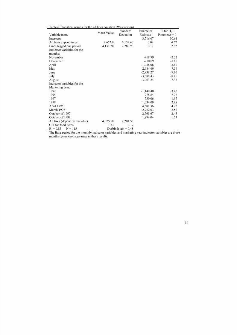
Table 6. Statistical results for the ad lines equation (West region)
Variable nameMean Value
Standard
Deviation
Parameter
Estimate
T for HO:
Parameter = 0
Intercept 3,716.07 10.61
Ad buys expenditures 9,652.9 6,159.40 0.09 4.57
Lines lagged one period 4,131.70 2,288.90 0.17 2.62Indicator variables for the
months:
November -918.99 -2.32
December -710.09 -1.88
April -1,038.08 -2.60
May -2,684.60 -7.39
June -2,938.27 -7.65
July -3,388.43 -8.46
August -3,063.24 -7.38
Indicator variables for the
Marketing year:
1992 -1,140.40 -3.421995 -978.84 -2.76
1997 730.06 1.97
1998 1,034.09 2.98
April 1995 4,588.36 4.22
March 1997 2,752.03 2.53
October of 1997 2,761.67 2.43
October of 1998 1,884.04 1.73
Ad lines (dependent variable) 4,075.80 2,281.50
CPI for food items 1.53 0.12
R 2 = 0.83 N = 115 Durbin h test = 0.48
The Base period for the monthly indicator variables and marketing year indicator variables are those
months (years) not appearing in these results.
7/17/2019 Aaea Paper
http://slidepdf.com/reader/full/aaea-paper 26/30
26
Table 7. Estimated demand elasticities
Mean Value Elasticities
Quantity demanded in pounds per million
people727,389
Own price elasticity (real terms):Pretail * (1-adexp) 0.641*0.56 -0.113
Adprice*adexp 0.462*0.44 -0.064
Total own price elasticity 0.56 -0.177
RINC (real terms)
Midwest 14,484 0.04
Northeast 17,684 0.08
Southeast 14,377 0.04
Southwest 14,411 0.06
West 16,203 0.04
Cross price elasticity, Washington apples
with:Banana1 0.12
U.S. pears (0.120) 0.006
Imported pears (0.406) 0.021
All pears 0.262 0.027
Imported apples 0.048 0.008
Cross quantity elasticity (quantities
expresses per million people):
WA-New York apples 333,308 -0.012
WA –Michigan apples 466,444 -0.018
Total WA- New York and
Michigan apples 799,752 -0.030
Advertising and Promotion elasticities
(expressed in real terms and per million
people):
TV 1460.80 0.006
Radio 803.90 0.003
Total Non-trade strategy (TV and Radio) 2,264.70 0.009
Demos 10.86 0.003
Display 27.59 0.008
Give-Away products 9.69 0.003
Total trade Strategy (demos, display, give-
away products)48.14 0.014
Other promotional expenses 21.47 0.002
Ad Lines 2927.30 0.066
Proportion of ad lines containing a logo 0.759 0.069
Proportion of ad lines in color 0.795 0.107
Proportion of Fuji 0.031 0.022
Proportion of Gala 0.205 0.069
7/17/2019 Aaea Paper
http://slidepdf.com/reader/full/aaea-paper 27/30
27
Table 8. Statistical results for the supply function
Variable name
Mean
Value
Standard
Deviation
Parameter
Estimate
T for HO:
Parameter = 0
Intercept 65.313 1.310*
PFR t (F.O.B. price) 0.331 0.049 498.261 3.900
PFR t-1 0.329 0.057 -219.301 -3.220Inventories in millions of lbs. 2229.000 1337.900 0.007 2.450
Exports lagged one period in
millions of lbs.
82.629 30.739 -0.278 -2.750
Apple producer prices paid index 1.032 0.178 -45.134 -2.590
Processing price per lb. lagged one
period
0.053 0.045 -339.090 -2.880
T 6.500 3.467 78.508 8.580
T2 54.167 46.292 -17.234 -11.970
T3 507.000 553.900 0.949 13.710
Mexican exchange rate X Mcrisisa 1.642 2.210
Weighted Asian Exchange rates 17.408 1.713 2.341 1.890
Large crop year indicator 0.300 0.460 37.915 7.330 Indicator for November and
December of 1993 and January and
February of 1994 (calendar year)
-25.546 -2.240
Total supply in millions of pounds
(Dependent Variable)
198.7 40.519
R 2 = 0.812 N =119 Durbin-Watson Test = 1.881
* Non significant at the 0.10 levela Mcrisis is an indicator variable with 1 from January 1995 through August 1995 (calendar year), 0
otherwise.
7/17/2019 Aaea Paper
http://slidepdf.com/reader/full/aaea-paper 28/30
28
Table 9. Statistical results for the Retail-F.O.B. price transmission Equation
Variable name
Mean
Value
Standard
Deviation
Parameter
Estimate
T for HO:
Parameter = 0
Intercept -0.243 -0.890*
Pretailt-1*Midwest indicator 0.204 0.400 0.150 1.260*
Pretailt-1*Northeast indicator 0.213 0.440 0.096 1.200*Pretailt-1*Southeast indicator 0.195 0.399 0.351 3.310
Pretailt-1*Southwest indicator 0.185 0.374 0.234 2.890
Pretailt-1*West indicator 0.194 0.385 0.345 3.630
Accumulative increases in F.O.B.
prices (PFI)
0.686 0.302 1.018 9.180
Accumulative decreases in F.O.B.
Prices (PFF)
-0.693 0.316 0.928 8.360
Wage x Midwest indicator 0.903 1.767 0.119 2.340
Wage x Northeast indicator 0.827 1.706 0.120 2.490
Wage x Southeast indicator 0.838 1.713 0.104 2.090
Wage x Southwest indicator 0.864 1.735 0.115 2.350
Wage x West indicator 0.890 1.757 0.070 1.440Transportation cost (TC) x Midwest 0.882 1.723 0.115 2.880
Transportation cost x Northeast 0.816 1.678 0.155 3.500
Transportation cost x Southeast 0.827 1.687 0.088 2.050
Transportation cost x Southwest 0.849 1.702 0.092 2.270
Transportation cost x West 0.871 1.716 0.114 2.740
Mexican Crisis indicator (MC) -0.006 -2.060
PC sales0.05 1.509 0.448 -0.034 -3.200
October 0.031 1.860
November 0.054 3.060
December 0.055 2.970
January 0.070 3.850
February 0.076 4.190March 0.077 4.060
April 0.080 3.950
May 0.108 5.00
June 0.118 5.340
July 0.071 3.230
August 0.079 0.021
Retail Prices (Dependent variable) 0.990 0.1086 Durbin h = 2.15
R2 = 0.715 N =359
*Non significant at the 0.10 level
September is the base period for the monthly indicator variables.

7/17/2019 Aaea Paper
http://slidepdf.com/reader/full/aaea-paper 29/30
29
Table 10. Simulated Average industry returns for the non-price promotional efforts
Marketing
Crop Year
Trade
Activities
Non-Trade
Activities
1992 17.83 2.421993 22.67 3.07
1994 25.59 3.63
1995 28.35 4.20
1996 28.99 3.48
1997 30.02 3.91
1998 30.26 2.15
1999 39.62 2.64
Trade activities includes demos, display, give-away products, ad buys/print media, and other promotional
activities
Non trade activities includes TV and Radio

7/17/2019 Aaea Paper
http://slidepdf.com/reader/full/aaea-paper 30/30
Appendix Table 1 Data sources
Information from the Industry: Specific Source:
Domestic shipments and Exports USDA, Federal Inspection Service, Unloads
Reports provided by W.A.C.
Regular retail price W.A.C.. “Marketvu” reports
Ad price, ad exposure, ad lines, ad with logos
and ad lines in color, market shares, accountshares
Ad Activity Report of a subsidiary of Leemis
Marketing provided by W.A.C.
Advertising Expenditures W.A.C.. Requisition reports and McCann
Erickson. Internal data
Information from other Sources: Specific Source:
State disposable Personal Income U.S. Department of Commerce, Bureau of
Economic Analysis
State population U.S. Department of Commerce, Bureau of
Census
Import data USDA, FAS World Horticultural Trade and U.S.
Export Opportunities Report. Various issues
Michigan, California, and New York
Domestic Shipments
USDA, Agricultural Marketing Service, Fresh
Fruit and Vegetable Shipments, Various issuesReturn to growers for pears USDA, ERS, Fruit and Tree Nuts Annual Report.
Various issues
Consumer price index for non food items U.S. Department of Commerce, Bureau of Labor
Statistics (see references for Series ID)
Producer Price index for TV and Radio
Broadcasting and newspaper publishing
U.S. Department of Commerce, Bureau of Labor
Statistics (see references for Series ID)
Wages and transportation index USDA, Agricultural Outlook. Various issues
Consumer Price Index (Chicago, Dallas
Miami, Los Angeles, New York, Boston, and
Philadelphia
U.S. Department of Commerce, Bureau of Labor
Statistics. Consumer Price Index (see references
for Series ID)