Aalborg Universitet

Why do we not have a Consistent Design Method for Rubble Mound Breakwaters

Burcharth, Hans Falk

Publication date:1985

Document VersionAccepted author manuscript, peer reviewed version

Link to publication from Aalborg University

Citation for published version (APA):Burcharth, H. F. (1985). Why do we not have a Consistent Design Method for Rubble Mound Breakwaters: Onthe Reliability of Rubble Mound Breakwater Design Parameters. Paper presented at Orgaan voorpostacademish onderwijs in de technische wetenschappen. Sectie Civiele Techniek en Geodesie. CursusGolfbrekers, Netherlands.

General rightsCopyright and moral rights for the publications made accessible in the public portal are retained by the authors and/or other copyright ownersand it is a condition of accessing publications that users recognise and abide by the legal requirements associated with these rights.

? Users may download and print one copy of any publication from the public portal for the purpose of private study or research. ? You may not further distribute the material or use it for any profit-making activity or commercial gain ? You may freely distribute the URL identifying the publication in the public portal ?

Take down policyIf you believe that this document breaches copyright please contact us at vbn@aub.aau.dk providing details, and we will remove access tothe work immediately and investigate your claim.

Downloaded from vbn.aau.dk on: juli 27, 2018

Orgm roor porwdemirh ondcrrij, in de Mnirbe wetemchappen 8- CIVIELE TKXNEK EN OEODE6lE

Cuuun OOWBREKERS lactun by

Ham F. Burcharth Department of Civil Engineering University of Aalborg, Denmark

September 24,1985

WHY DO WE NOT HAVE A CONSISTENT DESIGN METHOD FOR BUBBLE MOUND BREAKWATERS

(On the reliabiity of rubble mound breakwater d m pfumeters)

1. INTRODUCFION

The titJe of my lecture might be a surprise to many professional engineers. Is it really poss that we do not have a consistent design method - after several hundred years of breakwater sign and construction and also intensive research for the last 20 years? The answer is yes. state of the art and the design toob are not satisfadory compared to those available in o branches of civil engineering such as for example structural engineering.

I shall try to explain the difficulties we are facing in breakwater engineering, especially for rubbl mound breakwaters, by summarizing nome of the uncertainties we have to deal with in the process. A good overview of the uncertainties and the related consequences is of paramo portance to the designer. Without such knowledge it is impossible to evaluate the safety of structure - a situation that is unacceptable for a professional engineer.

It is important to point out that the damage to a breakwater never depends on one ter such as for example the wave height. Moreover, the time W r y (duration) of importance. This means that a discussion of uncertainties in breakwater design really sh based on the joint p robab i i density functions of the involved parameters supplied with cal information on the related persistance.

.The following presentation is not in accordance with this since each parameter is ly. This is done for the sake of simplicity and also because it will still serve the presentation. . 2. BASIC NEEDS IN DESIGN I

For most civil engineering structures (buildings, bridges etc.) it is possible to design and check the structud performance by means of theory. This is because many years of re- search and experience have established the prerequisites which are

Information on size of all major types of loads, often stated in standards as cha- racteristic maximum and minimum values, which- again are based on information of the statistical properties such as mean, standard deviation and

\

$dribution.

Info~matwn on the structuml response to the loads, implemented in formulae which are-in most cases the outcome of theories based on basic physics, but are in some cases more or less empirical.

Both loads and tbe response to those loads are known quantitatively to such an extent that meaningful safety factors canbe specified in the various standards.

Although this is well known to all professional civil engineers, it is deliberately mentioned here as a reference for the following d i i i o n on rubble mound breakwaters, for which the situation is compktely different.

2 .

3. ENVIRONMENTAL LOADS

3.1 Waves

The ideal situation, depicted in Figure 1, where both short term and long term wave stati­stics can be established from on- the- site records almost never exists.

AMPLITUDE RECORDS POWER SPECTRA CHARACTERIST IC WAVE PARAMETERS

~vJ"' .. -...c..A__,., __ .. Hmox. Hs. f ............. correct ion for shallow water effects etc .

>VJ\f'vi'IJ'1a, .. -~A<......>. __ .. H mox . H s , T .............. --

• • 'N'n(f-J'A .. _A.__""""-_ .. H mox 'Hs .T , .......... .. . --

LONG TERM (EXTREME ) STATiSTICS

DESIGN WAVE CLIMATE

PRELIMINARY DESIGN CALCULATION OF ARMOUR STABILITY ETC.

MODEL TESTS OF PRELIM INARY DESIGN

FINAL DESIGN

Figure 1. Ideal procedure for the establishment of design wave climate.

Usually one has to establish design wave conditions by hindcasting from meteorological observations and/or some wave records covering relatively short periods. In some areas visual wave observations from ships are available too.

It is clear from this that it is not possible to get reliable statistical values for all the wave parameters of importance. These are wave heights H, periods T, spectral shape, groupiness, direction of propagation and duration of storms.

Let us examine the wave height. This is generally the most important parameter since cover layer stability in terms of block weight is more or less proportional to the wave height

3.1 al

ve ;s,

ce :ht

3.

in the third power. The uncertainties in the determination of extreme wave heights may result from the following sources:

A. Errors in measurements, visual observations or hindcasting of the wave data on which the extreme statistics are based.

B. Errors related to extrapolation from short samples to events of high return periods, i.e. low probability of occurrence.

Errors due to the choise of exceedence level. Errors due to the method of fitting data to a chosen distribution.

C. Lack of knowledge about the underlying distribution for the extreme events .

D. Errors due to plotting positions.

E. Climatological variations.

ad A . Errors in wave data

Le Mehaute et al. , 1984 discussed the uncertainties and systematic errors or bias related to the wave data under the assumption of errors being normally distributed . They reported the fo llow­ing "typical" normalized standard deviation a' defined as the absolute standard variation divided by the expectation ("mean") value of H

5:

Direct wave measurement aM = 0.05 bias 0.00

Visual observations from ships aM= 0.20 bias 0.05

Hindcast (excluding hurricanes and other tropical storms) aM= 0.15 bias 0.05

It should be noted that the two last set of figures are applicable only when the sample popula­tions are ranked statistically. A direct comparison in the time domain, i.e . comparison of indivi­dual sea states, generally shows larger discrepancies. Moreover the figures are average figures. For instance it is believed that wave data based on to<iay's most advanced hindcast models applied to relatively restricted areas, such as the North Sea, where high quality weather maps are available, will show a smaller uncertainty.

ad B . Errors due to short samples.

Estimates on events of low probabilities are often performed in the following two different ways:

1) The extrapolation of data from frequent measurements or observations. The data are often compiled at intervals c. t = 3, 6 or 24 hours, which gives a large sample, N events, even in the case of a short time of observation or record length Y in years. The order of magnitude of N is often 1000 - 10,000.

2) The extrapolation of relatively few data sets representing the max significant wave height H

5 for a number of storms exceeding a certain level, H~. The data are often de­

termined from hindcasts and the sample size N is typically within the range 10- 30.

Wang et al. , 1983, examined the uncertainties related to the first method. They considered the long term distribution of H

5 to be of the exponential type which also includes the often used

Weibull distribution,

(1)

where A is signifying the background noise level or lower-bound, B is the scale parameter and"! is the shape parameter. All three characteristic variables are ,.. ormally determined by best fitting to the observed data.

4.

Assuming the data asymptotically normally distributed about the underlying probability distribu­tion function , eq (1), the authors obtained for large N the normalized standard deviation,

(2)

where R is the return period in years, v is the number of observations per year compiled at inter­val At and Y is the number of years of observations. Formula (2) is valid only for low proba­bility levels and only for large samples N = 11 Y of uncorrelated data. The latter implies that ..l t should exceed approximately 24 hours, but because of little sensitivity on the confidence bands for H

5 smaller values, as for example At = 6 hours , are often used.

It is stressed that the data to be used must belong to the same statistical population as the ex­treme events in question, i.e . wave data must be separated with respect to origin or type of waves, to directionality , to shoaling effects etc.

Example.

Taking R = 50 years, Y = 5 years, 11 = 365 observations per year and 'Y = 1.2 gives a~ = 0 .27

Changing R and Y to 100 years and 3 years respectively gives a~ = 0.46

The second method mentioned above is relevant to situations where data have to be obtained from hindcasting, which , due to the costs involved, restricts the number of data.

Rosbjerg, 1981, considered this case, where only maximum values 11 of H5

for independent storms exceeding a chosen level H; are taken into consideration, cf. figure 2 .

H ' s

+--------------L----------~------~~ TIME

Figure 2. Data reduction by application of exceedence level, H;.

Rosbjerg assumed all the exceedences 11 - H; to follow the exponential probability distribution,

H -H' P(H) = P[17 ~ H5]=1-exp(-

5 5)

s a (3)

which is of the same type as the Weibull distribution, eq (1), with 'Y = 1.

The author also assumed the events 17 to occur at times corresponding to a Poisson-process with time dependent intensity. He arrived at the following expression for the R-year event defined as the value of 11 , which in average is exceeded once every R years,

H = H' + a ln11 R s s ( 4)

>U·

;er­ba­.H

nds

ex­~ of

ined

::>rms

;ion,

(3}

ss with ined as

(4)

The corresponding absolute standard variation is

a = a (1 + (lnv R) 2 ) 0·5 s (V Y)0.5

and the normalized standard deviation consequently

__ a _ _ (1 + (lnvR)2 ) 0 ·5 , as ( v Y) 0.5

as = H5

= ..:.._---'---:-:H,.,-; -+-a....,l_n_v_R __ _

The maximum likelihood estimate for a is

a= ii - H' s

where ii means average of 11 .

Nielsen et al., 1985, extended the analyses to include the Weibull distribution

H5 -H~ P(H) = P[17 ~ H 1 = 1-exp(- ( )"Y )

s s a

and found the following

Cl .

(5)

(6)

(7)

(8)

(9 )

lh-1[ a 2

a = (lnv R) ~y + (lnv R) 2

S 'f V

2 2 f (1 +-) 2 ]05 a a · y ( 1 - 1) + 4 (lnv R) ·ln(lnv R))2 Var[ .Y 1

v r 2(1 + -) r 'Y

v is the average number of data per year and r the Gamma function .

The variance of .Y, V ar [ .Y], cannot easily be estimated, but by means of numerical simulation it is found that the term in (10) containing this quantity is highly dependent on the method for esti­mating the parameters in the Weibull distribution.

Petrauskas and Aagaard, 1971, found , by using a least square method, that the last term in (10) is insignificant. In this case the normalized standard deviation is

2 l.-1[ a z a2 f(1 + -) ] (lnvR)"Y ~y + (lnv R)2 -y ( 1 -1)

aS 'f V V f 2 (1 + - ) a~ = -Hs :: _______ H_'_+_ a_(-ln_v_R_)-:

1-:-h _ ____ 'Y'----

s

(11)

Nielsen et al. , 1985, fitted the Weibull parameters by the method of moments, i.e. equating the first three moments of the distribution to those of the data, and found that the last term in (10) was of significance, namely in the order of 1/3 of the total standard deviation. The estimates on the parameter by the applied method of moments are given by

(12)

(10)

--.v-:--

6. - 62 . qa - (3'

2 1 (18) r ( i + ~ ) - r = ( i + 7 )

7

*:, . 1 Q = { - & I - ( l - r ) 7

(14) .. . ~. - ---- -~ . . ~.

7 and 7 maan tbe amage of ample values of 9' and q' . respectively, which are unbiased eeti-

'*. matesof E[qa1 andE[q3 I . ..?

-. :,. It should be noticed that the R-year event given by eqs (4) and (9) ha8 a probability E of b e i i equalled or exceeded in the specific lifetime L of the stntcture. For instance, il L is set equal to

,', the retum period R, thin "encounter probabilitfi E is as large ae 63%. The ~e&iou.&~ betw&n :t R, L and E irigiven by .

~. ~ . - - 2 L

4 E = I - ( I - ~ R o r i n a r o f R l a ~ g e R=-h(l-E) .~ . . . . ~ ~ . ~~ .

(15) - - ~ . ~~. -.

For design purpose R in eqs (4) and (9) should be evaluated with mpect to E and L through eq (15). For example in a 50 years lifetime there is a 10% probability that the Btruchne is hit by the

- 500 years' return period storm. - .

Eqs (6) and (11) make it possible to determine the neeessay sample length when a prediction for a given return period with a prescribed accuracy and confidence is required. Following the nor- mal distribution the products of a; with 0.84,128,1.65 and 2.32 define the uppe~ bound of 6pread corresponding to a confidence level of 80%. 90%, 95%. and 9946, mpedively. For in- . stance, the prediction of an event with 90% confide- and an u n m of no more than 0.20 imply that 128 a; < 0.20. M i n g this in eqs (6) or (11) gkw the conespondiug number of years of observation Y for given v and R.

Example. The accuracy o? estimates based on a restricted number of hindcested data sets might be illustrated by the following example. The Delft Hydraulics Laboratory did a hindcast study for a specific deep water location in the Mediterranean Sea and found for a 20 yeam period the following 17 most severe storms, Table 1:

Tabk 1. Exampk of hindcasted storm wave &to for a 20 years'period.

Rank Max H, (= v ) Peak period T, Average wave direction i meters seconds degrees

Ifwe cham Hi = 4.0 m we find N-14 rrtomexo3edingthblevelovera@odY =20year~, which gives v = 14/20. Accordiog to eq (7) p! can be estimated to 6 = 2.00 m. It can now be teat- ed if the data follow the - distribution, for example the exponential type given by eq (3). In this a haight line with slope 1:l ehould be obtained by plotting qi - Hi again&

i - & h(1 - P(fii)), where P(Gi) = 1 - - N + l , (Gumbel plotting positions). Figure 3 shows that the Kt is reasonable.

Figure 3. Test on exponential distribution of wave height exceedences.

Formulae (4) - (6) are then valid and the expectation values and the standard deviations can be calculated for various return periods, for instance

Return @od R H~ OS O;

Y m meters m e W

Note that a change in H; for example to 3.50 m, which still gives N = 14, wil l change H, and o,! This important problem is not discussed further here.

It is obvious that the 14 data points also fit a Weibull distribution.

If all the 17 data points given in Table 1 are considered, it corresponds to a exceedence level of Hi e 2.25 m because the lowest value in the data set is H, = 2.33 m. It kuns out that in this case the data do not fit neither the exponential distribution, eq (13), nor the Weibull distribution, eq (8). However, if the exceedence level is not interpreted as the physically true cut-off level, but is

Figure 4. Data fit to the WeibuU distribution. Gurnbelplottingpositio~~

*. - . . ̂ --.-_.urr; .-----. :~.(r-Ui-Uiuriuria,~>:.a,iYIY~.-..U7~

<, .a '7%. * ~

regnrded a fitting coefficient only, like Q and 7, then the 17 d.tr points follow the W e b u l l distri- bution very dasely, u demonutrated in Figure 4. The oocffrienta are in th ia ccue H; - 0.79 m, CI = 5.27 m and y =2.80, all estimated by the method of moments.

A ~nl - ln i l -Piqi l l~

h m eqs (9) - (11) we obtain the following corresponding values

1 -.

0 -.

-1 .

- 2

- 3 7

Return period R *S "S a;

Y m meters meters

.: a / 3. 3

)In(rli -0.731

The Weibull distribution shown by the straight line in Figure 4 is a result of the chosen method + of fitting. A least square fit or a visual fit will produce different lines and different estimates on the extreme events. $

-,

t F

ad C. and D. Errors due to the lock of knowledge on the true long term distribution and due to s

plotting positions. 4 Several probability diitributions ate used to describe extreme wave height statistics. These in-

"is clude for example the log-normal distribution, the extremal type I or Gumbel or Fisher-Tippett I

.p 6

distribution, the extremal type II or Fretchet or Fisher-Tippett II distribution, the Wad-Bog- man distribution and the extremal type m or Weibull distribution Although each of these distri- butions has a theoretical bsse, they arnnot be evaluated and related to the extreme waves on a physical base. As a consequence they are only fit to the available data. Most often the scales used - for the plotting are such that the chosen distribution lies on a straight line, simply because of the

0 1 2 3

5 g 4 :,$i

ci · n ,

!thod .es on

.ata to

iue to

ese in· ?Pett I -Borg·

: distri· ~son a es used ! of the

9.

more convenient visualization of the extrapolation. However, when extrapolating, one should al­ways be aware of possible physical processes, such as for example wave breaking, which might in­terrupt the probability distribution at some probability level.

It follows from these comments that due to unknown extreme distribution errors can only be estimated by a sensitivity analysis in which various distributions are fitted. Table 2 shows such an analysis by the Delft Hydraulics Laboratory performed on the wave data given in Table 1.

Table 2. Example of influence of choise of extremal distribution and plotting position on low . probability wave heights. Data by Delft Hydraulics Laboratory.

Extremal distribution

Type I Gumbel

Ward/Borgman

Type Ill Weibull

Plotting position

Gumbel

Gringorten

Gum bel

Gringorten

Gum bel

Gringorten

Correlation coefficient

0.9875

0.9852

0.9872

0.9920

0.9877

0 .9877

Return period H5

50 year 100 year

11.0 m 12.2 m

10.3 m 11.3 m

9.8 m 10.5- m

9.4 m 10.1 m

9.6 m 10.2 m

9.3 m 9.9 m

Although no accurate figures can be given it seems reasonable from this table and the above given example based on the distribution, eq (3), that due to unknown extreme distribution a nor­malized standard deviation a0 might be in the order of

a 0 ~ 0.05 · 0.10.

In order to plot the data a position formula must be adopted. Many different plotting positions, all based on some statistical considerations, exist, but it is not easy or possible to select a specific one as the most correct. For this reason it is reasonable to estimate the error due to plotting posi­tions by sensitivity analyses involving a number of reasonable plotting rules.

Table 2 gives an example where only two plotting rules are used, namely

Gumbel/Weibull

and

Gringorten i- 0.44

P(7?i) = 1 - N + 0.12

(16)

(1 7 )

It is seen that significant deviations in the estimated extreme wave height occur due to the plot­ting rules. It is believed that a realistic normalized standard deviation a~ on extreme events will be in the order of

a' ~ 0.05 p

.=al-I[e=q $0 *sap am roa ~IqWP w ram qanm am saamosar asaq~, wan! aroqqo an@sord q? q .*a sagsg8p aaw 's3tq103ar anwa uo pads samosar am aqq wdsap w~a 4-rn\ !q i%91 T Xlal-dd~ Jo & -WmUlI UE q?W m 8Z SB& aq? P861 o! XIPCJ PW 'm P& o) dn-1861 a! !m 0'82 LL61 o! !m 9.~8 = $1 ZL~T q -m 9-61 a4 o) pa)--& ~Gaq a~m *sap mX 001 ar~ OL61 n~

'dwo~ 50 mnr~~,

iossajoq ~q ua~? pIag a~oqsg~o was WON qsgom m@amo~ aq? mog a~dmera ~~AOROJ am dq palm aq oq %q- q@aq u0 w~m!%93 ~IWW %mnI.elqo n! =F+FJW aq~,

'aAoq8 ua~p asow boIaq sam%g g paanpar are uogm -iasqo JO pouad aq% em sl8p jo sqWa1 aw -q* XI%W~J%~ ~~=a! 4uwaon aqL

'%q%aq pal- aq% sam~) 01'1 - SZ' 1 m? 1aVq Bmaq ?%aq anw arpl JO Q -@grrqord %.g1 B sugdm v safq-mopm pelnm d~oa anmsss aa n - ~2.0 = ,o JO

=pro aql m P- iuwwi? s! ?uw maX 05 aw o) pa)^ K?wwm am 'POW KPA=W pw a~dmm q~p JO sq@a1 aIq=uossw pepre%u Xwana8 q ?8q~ qly uada '?8w uaas ?! qqq moq

:sa[dmwa 04 Btqaonoj aw qqqqsa wa auo uo!ssnaqp Byo%ioj aql g aauaqa q11fi

2 '80.0 4 ?nsmX 001

lo 09 = pw 998 = n roj pug ah =owns aq3 Xq pasodoad ss 2.1 je L q8mq.w aamqsq ioj a& n I?-

(81) -. - (4X)'JlL= q, 1 5

1te et being gY= ; in R

( 18)

50 or

for an e data

( 19)

years.

a sample ;he order >robabili·

of obser·

trated by Professor

:3.6 m ; in mcertain· ton wave uch larger

11 .

It is not only the wave height that is of importance but also

• the wave period

• the spectral shape

• t he horizontal, directional spread of the wave energy I short crestedness of the waves

• the groupiness

• the direction of the propagation

• the duration I time history of the storms

Therefore the uncertainty related to the estimation of these parameters should also be evaluated. It takes a lot of work and research to perform such an analysis, also because generally it is the re­liability of the "joint parameters" which are of interest. This problem is not discussed further here. However, it is obvious that it all adds to the uncertainty on design wave climate est imations.

If the breakwater is in "shallow-water" and the wave data are from an offshore location then we have to include the uncertainty related to shallow water effects such as :

• Refraction, i.e. change of wave direction and wave height due to oblique wave ap­proach.

• Shoaling, i.e. change of wave height and wave length due to water depth variations per­pendicular to the coast.

• Wave breaking, due to instability by decreasing water depth.

• Wave set-up, i.e . change of the mean water level due to changes of the wave radiation stress.

Besides these effects we also have:

• Tidal water level variations. • Barometric pressure variations. • Wind set-up, i.e. wind induced change of the mean water level. • Seiches. • Currents.

The uncertainties related to all these parameters or phenomena are in general not well established except for tidal water level variations. Consequently a quantitive discussion on uncertainties is not possible. However, in the next paragraph we shall evaluate the importance of reliable data by a sensitivity analysis of the structural response to some of the parameters.

It has often been pointed out that estimates on design waves are much more reliable in shallow water than in deep water due to the depth limited wave heights. This is true but it should be mentioned that no wave theory exists which can predict with good accuracy the absolute wave height distribution and maximum wave heights in shallow water with breaking waves. Moreover, it should not be overlooked that the water level is also a very important parameter when break­waters are designed for a certain amount of overtopping.

Another point which should be stressed is the sensitivity of shoaling/ wave breaking to variations in the sea bed profile. This is illustrated in Figure 5, where the wave heights of the incoming waves at the toe of a breakwater are determined for four different foreshore bottom profiles. The breaker index 'Y , defined as the ratio of the max significant wave height, H~ax and the water

Hmax s

depth, d at the toe, is also given in the figure together with the breaker index 'Y H max related to the maximum value of wave heights, exceeded by 1% of the waves. 1 %

I

I

12.

d' -8.0 ____ _____; -20

--~~~-------------------,--------------------~~~-)Om

E 0 M

1000 m

1000m

SW L

SW L

SW L

SOOm

PROFI LE :;

500m

a, - 11 s

Jm TOE JF

3REA~WA7c'l

0

J.., - cE CF

BREAKWA TE<l

0

-10

-20

Gm TOE OF

3REAKWATER

-10

-20 -P-R-OF-I-LE--0----------------~ -.!-...-ri""'------==---------..--I------- --+--'-JCm

100Cm SOOm TOE OF'

BREAKWATER

H(m) AT TOE OF BREAKWATER

10

9

8 .. -··--· 0

H, ... ----- 8

H, 'lo 6

BREAKER INDEX H -e: '(

l : ----d

5 PROFILE AT TOE OF BREAKWATER

H, (m) OFFSHORE AT 30m WATER DEPTH

O L-+-~-+~-~~~-+~~+-~

0 3 I. 5 6 8 9 10

H, -- .H1-_,,---

A

B

c D

J M:'' l .,, ... ... 0 63 0 83

0 73 0 90

0 71 0 98

0 70 0 87

Figure 5. Example of sensitivity of depth limited wave heights to differences in foreshore

bottom profiles. Delft Hydraulics Laboratory.

13.

e wave beights wss determined by DHL in wind-nave flume model tedta without the W-

in seen that a good estimate on the wave height in front of a breakwater in shallow water must based on model tests with a correct reproduction of the foreshore topography. This mean8

case of significantly varying bottom topography along the breakwater it is necessary either many sections or preferably to t& the hole ~4~11eture in a thxee-dim&d mod&.

SENSITIVITY IN STRUCTUW RESPONSE M THE ENVIRONMENTAL LOADS

e following in not intended to be a complete discussion as only a few, but important, prob- ms wiU be discussed.

1 Hydraulic stability of the armour layer

difficulties related to a purely theoretical stability analysis might be illwtrated by consider- the forces on an armour unit, see Figure 6.

8 FlELOu=u(x.y.z.t)

Na -$ !. NOT KNOWN I

GRAVITY F,; gg,@ - 1) d3

FORM DRAG FDF = CF gw d21ulu

SURFACE DRAG FDS=Cs 9, d2 IU~U LIFT F L r CL 9 d 2 u 2

INERTIA. FROUDE- KRYLOV FI =CI gw d3u'(~res%re gmd d ~ s t u r b flow)

INERTIA. ADD HYDRODYN MASS F,=Crg,d3 u'(charge of flow fleld by the

COEFFICIENTS C ore funct~ons of Kwlegon- Carpenter No and Re NO and wlll

vary conslderdy in tlme

re 6. Forces on armour unit.

ence stability formulae are semiempirical and formulated as an equality between a ristic drag flow force and the stabilizing gravity force multiplied by unknown functiolu

take care of slope angle, on, interlocking, wave period etc.

't!un mowo jo ip 'smtu

pajnbai uo H 'jqaaq mom jo aauanuu~ .L =''ad

'6 qd- .p 'H 8'0 sp uaqs) a (H) o -moqs g (H) o T H a- aq$ a! n JO uogw wgqa aql amq~ ru'~ am&l ri! ~~dap ? .qq@aq am no sqmqsa aspwd IOJ paau aql uo sp~sqdma ~nd ~r~padap Woay kea .ad pqq aq7 rr! $q-q aq$ g paogodad ssalro =om q $!un moma aw 30 yy 'raw mbar JO mm 4 Xmqw aq? 7~~1 aoqs aslnmo~ snow aq~,

'9L61 -WV PM '6961 'lawox 9 !ua Kq ~qdq -dm-& pun raro3r mouuu uuoj!un jo rsmu pa+nbat uo mad mom jo amand y jo .aldurmg

-or =*d

- -

- - --

'diu-du XOJ m'spaaq qmdo #w inq 'am pw sauv mrom go am aw y wms m popad ah= o) &p!m-~= 454~ aq7 7W sli1.9L61 'mWV 'du-du Pm 6961 'pmq 0 Fa 'sauv -om WP =A= q@a a! 878al4!1!9s)s $0 301da 8 -0qS 01

'poyad aaua aqq qq~~ X[~W~~TJ?S ~a88a3q dn-rmr iq woqs oap aauaagaa am au '6 'sa~~fi qn8a.x o) pasodxa mom asso~oa ww slsa)

a! 6,561 '- Xq POI a3~p-p 3- IlW in9 iqaamw V

16.

I

I I

In Figure 11 the data are normalized with respect to r = 3 for easy mutual comparison of the wave period sensitivity. r = 3 is a characteristic average value for rubble mound breakwater design wave situations. It is seen that an uncertainty on T (for example a'(T) = 0.15) around the value T

1 = 3 only gives relatively small variations on the required mass M.

This is somewhat contradictory to Figure 8 but might be explained by the influence of the wave wall as explained above.

Figure 11 also shows that the larger the porosity of the armour layer t he more vulnerable the ar­mour is to large wave periods (Dolos armour has the largest porosity and rip -rap the smallest). This is due to the " reservoir effect " of the pores as explained in Burcharth et al., 1983. A stabili­ty minimum seems only present for the relative impermeable rip-rap.

Note that the data in the Figures 9 , 10 and 11 are from tests with regular waves.

2. 5

2.0

127. 5 21 I H . 551

DOLOSSE cot a , t 5. BURCHARTH, 1979

TH RESHOLD OF ROCKIN0

v--DISPL ACEMENT OF FEW UNITS

I I

I

[!] I [!] 7 "' Z/ UNIFORM ARMOUR STONES,cotao 15

OAI & KAMEL, 1969.

1.0 t------tr.ii~~- ~ - .. .. . .. . .. .. ... . .. .. ... ·;;. " "7 "" /RIP· RAP.co t a' 2 . 5. AH RENS. 1975

[!] ~-<6 0 .5 ........ [!]

13 ............... -[!]

T 0 +----+----~--~~---4---.

o 0.5 1.5 r~o~

1,.RELEVANT RANGE FO R .,1 RUB BLE MOUND BRE AKWATER

Figure 11 . Example of influence of wave period on required mass of armour units and rip -rap. Regular waves. Data normalized with respect to the estimated values A A g 0.5 T

1=

3 and M

1= 3 corresponding tor= T ( 2rrH) tana = 3.

The examples show that the effect of the wave period on armour stability is not clarified in

general.

4.2 OVERTOPPING

The design conditions are often related to overtopping of the breakwater. This is the case where roads, reclaimed areas, berths, installations etc . are located behind and close to the breakwater.

Overtopping is very sensitive to variations in wave height and mean water level. Besides this also variations in wave period, wave direction and wave shortcrestedness affect the overtopping.

The sensitivity to the wave height can be illustrated by the example given in Figure 12, which shows some scale model test results from a rubble mound breakwater with a wave wall.

the ·sign alue

Nave

1e ar­lest). abili-

-ip-rap. values

rified in

;e where akwater.

this also lg.

2, which

Figure 12.

! OVERTOPPING. Q

J0 -1

I zs-r

20-

I 5 -i-

I st

LITRE PER SEC PER METRE • 54E~ 3E: ;,o-;:= _::: 3

.. :e: ~- - ·: :o:: .... :.-:l:~- ~ ... :; 2.-

C~EST :.r ·~ ;Jm

· ;Cl ~;; :~:.:~: .o :

Cl

:RESY ~ "!' · 'V :-.

17.

Example of sensitivity of overtopping to wave height. Delft Hydraulics Labora­tory. Sea bed profiles refer to Figure 5. o I

__ 0 /0

5E• 3E~ oqCi'L 'O •

Cl _// "OE ~T ·! Jm a-•V ~•--• ·•c·r ·· ~/. .-- ~"-' ;r., .. -

.~...,........ -1 • 1 "' s •o H, ( m ) At 30m

WATER DEPTH

It is seen that the overtopping, Q increases exponentially when the wave height exceeds a certain value. A 10% increase in H

5 can easily cause doubling of Q. The exponential growth of Q with H

5

usually makes logQ a linear function of H5

•

Based on different scale model experiments Jensen et al., 1979, presented a more general descrip· tion by means of the parameters QTz /B* 2 and HJ~h. T z is mean zero crossing wave period, B* is a representative horizontal dimension and ~his the vertical d~tance from still water level to the top of the crest or wave wall. By introducing ~h also the influence of water level is taken into account. Figure 13 shows an example given by Jensen et al.

Figure 13 clearly shows that even small variations in the still water level might cause significant variations in overtopping.

10;+--1---+--+---+---. ~ 0 0 2 0 4 0.6 0.8 ll h

ARM OU R: TWO LAYERS OF TETRAPOOS

WINO SPEED " u• _ u_= 1.8 ~

0 OVERTOPPING IN M1/S / M

T, MEAN WAVE PERIOD

H, SIGNIFICANT WAVE HEIGHT

Figure 13. Example of sensitivity of overtopping to wave height and still water level. Shallow

water conditions. J ens en et al .. 19 79.

18.

4.3 Directionality of the waues

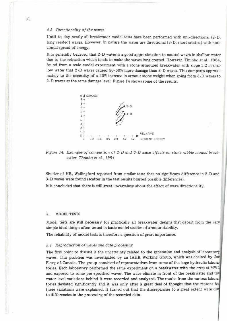
Until to day nearly all breakwater model tests have been performed with uni-directional (2-D, long crested) waves. However, in nature the waves are directional (3-D, short crested) with hori­zontal spread of energy.

It is generally believed that 2-D waves is a good approximation to natural waves in shallow water due to the refraction which tends to make the waves long crested. However, Thunbo et al. , 1984, found from a scale model experiment with a stone armoured breakwater with slope 1:2 in shal­low water that 2-D waves caused 30-50% more damage than 3-D waves. This compares approxi­mately to the necessity of a 40% increase in armour stone weight when going from 3-D waves to 2-D waves at the same damage level. Figure 14 shows some of the results.

% DAMAGE

9

8 , ' ,

7 %.2-0 I I

6 , 3-0 5 , ,' I I

I. I I I

3 I

·--' 2 1

RELATIVE 0

0 0. 2 0. , 0.6 0.8 1.0 1.2 INCIDENT EN ERGY

Figure 14. Example of comparison of 2-D and 3-D wave effects on stone rubble mound break­water. Thunbo et al., 1984.

Shutler of HR, Wallingford reported from similar tests that no significant difference in 2 · D and 3 · D waves were found (scatter in the test results blurred possible differences).

It is concluded that there is still great uncertainty about the effect of wave directionality.

5. MODEL TESTS

Model tests are still necessary for practically all breakwater designs that depart from the very simple ideal design often tested in basic model studies of armour stability.

The reliability of model tests is therefore a question of great importance.

5.1 Reproduction of waves and data processing

The first point to discuss is the uncertainty related to the generation and analysis of laboratory waves. This problem was investigated by an IAHR Working Group, which was chaired by Joe Ploeg of Canada. The group consisted of representatives from some of the large hydraulic labora· tories. Each laboratory performed the same experiment on a breakwater with the crest at MWL and exposed to some pre-specified waves. The wave climate in front of the breakwater and the water level variations behind it were recorded and analyzed. The results from the various labora tories deviated significantly and it was only after a great deal of thought that the reasons fo these variations were explained. It turned out that the discrepancies to a great extent were du to differencies in the processing of the recorded data.

2-D,

hori·

vater .984, shal­'roxi· res to

break·

-D and

the very

boratory j by Joe

.c labora· ; at MWL rand the 1s labora· asons for were due

19.

5.2 Scatter in test data

Another problem in model testing is the scatter in the test data signifying the response to the waves. This can be illustrated by some stability tests performed at the University of Aalborg with a Dolosse armour layer having a slope of 1 _in 1.5 and exposed to irregular waves. For each of five different significant wave heights, H

5, 15 tests with identical wave trains were run with the ob­

ject of studying the movements in terms of rocking and displacement of Dolosse. Very careful visual observations were made simultaneously by four people each covering a small area. A mir­ror system was used to obtain reliable observations in the splash and underwater zones. Each test was run for 20 minutes corresponding to approximately 1200 waves.

Some test results are shown in Figure 15, which illustrates the observed scatter related to the number of rocking and displaced blocks. These two modes of movement are relevant to the me­chanical integrity of the blocks and the hydraulic stability of the armour layer.

Although direct recording of stresses in and/or recording of speed/acceleration of the blocks are much better than visual observations, the diagrams clearly illustrate the fact that reliable esti­mates of stability can be obtained only when tests are repeated several times. This is a fact which should not be overlooked.

It means that it might be necessary to apply a large safety factor if only a few tests are carried out, or to spend a lot more money performing many more tests than is normally the case-at the moment. This is especially true for the complex, fragile types of armour units since it is seen from the Figure that the normalized standard deviation a /JJ. for the numbers of displaced units is very large for small degrees of movements or damage corresponding to the design criteria for such units.

For large degrees of damage, i.e. failure situations, the scatter is reduced.

It should be mentioned that separation of rocking and of displacement in the "two" diagrams is not entirely meaningful and should be avoided in design diagrams. It is also important to remember that the scatter (e.g. in terms of the standard deviation) is dependent on the size of the test sec­tion.

5.3 Scale effects

The reliability of breakwater scale models has often been and still is seriously questioned and in most cases exclusively with reference to scale effects (thus forgetting the afore mentioned points). All scale models involve improper representation of some forces simply because only two types of forces at a time can be represented to scale. Therefore the question is "how much" is the model biased.

The two dominating forces in wave action models are gravity and inertia forces. Considering only these two types of forces the Froudian model scale law used for breakwater models ensures dyna­mic and kinematic similarity of the scale model and the prototype. Consequently viscous forces and surface tension are not reproduced to scale.

Viscous effects For a wave exposed breakwater the flow is extremely unsteady. In some parts of the porous structure the flow will be turbulent or laminar all the time but in some part intermittent between the two flow-regimes, as discussed by Burcharth 1983.

The turbulent dragforces will scale like the inertia forces, because the viscous contribution is in­significant.

The flow-regime in granular structures is usually characterized by a Reynolds' number defined as

IR=Vd V

(20)

DISPLACED BUXXS IN TESl AREA A (AROUND M W U

I

2.0 + c V ROCKING BLOCKS IN TEST AREA A (AROUND M W L )

K T U A L RELATIVE NUMBER f. NUMBER(%)

LEGEND:

EACH W T REPRESENTS TEST SECTIONS ONE TEST.

H, SIGNIFICANT WAVE HEIGHT.

h HEIGHT OF DOLOSSE.

p MEAN VALUE

U 5TANDARD DNlATlON

WAIST RATIO OF DOLOSSE 0.32.

ENSlTY OF WLOSSE 228 t/m3

WIDTH OF WLOSSE TESI SECTIMIS I S 9h.

NUMBER OF COLOSSE IS 60 IN SECTION A AND 81 IN EACH OF YCT IONS B ANDC.

Figure 15. Example of scatter in amour stability tests.

21.

where V is a characteWc flow velocity, d is a characteri&ic length and v the kinematic viscosity of the liquid. When evaluating the unsteady flow in breakwaters it has become a W t i o n to use a constant figure for V which, more or less, is the maximum particle velocity of the incoming wave, i.e. V = (g H)", where g is the gravitational constant and H is the wave height. d is usually taken as a typical diameter of the armour units/filter layer stones/core material, thus charade- rizing the width of the flow channels.

The primitiveness of this approach is obvious, but it is difficult to come up with an alternative which is both meaningful and simple. - - - -- -

Many researchers have studied vkous scale effects in breakwater mopels and the date of the art - - .- might be summarized as follows:

a No "signficant" scale effect is observed in the "hydraulic stability" of the armour layer if R > 1 - 3.10' (d being a characteristic diameter of the annow unite) and if the filter stones and the core material are geometrically to scale.

However, it is important to notice that this statement is conclusive only in reletion to mechanically strong armour units such as for example natural stones and concrete cubes. For the more fragile, complex types such as Dolosse and Tetrapods a scale ef- fect which is not identified from visual observations of armour unit movements in the model might, when transferred to prototype, cause a very different amount of break- age. Timco et al., 1984, investigated this in some tests with Dolosse units with correctly scaled mechanical properties. They found that the influence of core permeability on the breakage of the Dolosse was very dependent on the geometrical d e .

Run-up and overtopping are affected also by the porosity of the filter layer and the core. It has not been properly investigated how much changes in the size of the stones in order to obey the Reynolds' criteria stated above will bias run-up and overtopping.

The reflection of waves from a breakwater scale model is practically independent of the permeability of the core, Timco et al. 1984.

There is evidence that u l t ' i t e failures of rubble mound structures armoured with strong units can be studied with great accuracy in kale models. This statement is main- ly based on a comparative study by DHI, Jensen et al., 1985, . of the failure of the Thorshavn breakwater in the Faroe islands. This study is significant because of the availability of the prototype records of the waves in front of the breakwater through- out the damaging storm. The Reynolds' numbers in the model were about 4-10' for the m o u r stones and about 5 .lo3 for the quarry run which eventuslly was exposed to the waves.

Very little is known about scale effects related to the flow and the pore pressure in the more impervious parts of the breakwater such as the core (and the seabed if of sand). This means that for example uplift forces on concrete cappings and geotechnical aspects such as slip-circle stability and settlement cannot be properly evaluated in a scale model at the moment.

Surface tension effects I The surface tension determines the amount of entrapped air in breaking waves. As a consequence I

scale effects are present in scale mod& of forces from breaking waves and overtopping/spray. The shape (surface profile) of the waves in very small scale models is also affected. I

Stive, 1985, studied the influence of air entrainment in a comparative scale model W y of waves breaking on a beach. He recorded wave heights, set-up and vertical profiles of maximum seaward, maximum shoreward and time-mean horizontal velocities and found no significant deviations from the Froude scaling in a wave height range of 0.1 meter to 1.5 meter. This indeed indicates

22.

that surface tension scale effects are higniflcant even in small scale models except for phenom- ,

e m where a very scculste r epdud ion of the 1no6fe of tho bmaking wave is important. TIM most important example is shock pressurea on plane solid nails. A special problem related to shock pressures is the interpretation of the recorded pressures in the model, because the air com- pressability is not to scale. This problem has been disc& by many researchers, see for example Lundgren, 1969, but it still remains to check model data against prototype measurements before the uncertainty related to ehock pressures can be evaluated.

However, the author believes that the order of magnitude of wave pressures on wave walls found from proper scale models is correct. This opinion is based on a study of breakwater failure where damage to the concrete capping with wave d - d o w e d a rather accurate determination of the wave forces involved. By means of results from scale model tests, performed by DHI, in which wave pressures on the wave wall were mlded, it was possible to estimate the wave climate. This estimate was in very good agreement with the wave climate established by hindcast from mete- orological observations.

Effects of mechanical properties of armour units The relative strength of armour units is dependent on the size of the units, Burcharth, 1981. This has to be taken into account when designing and interpreting the scale models. The importance of this has been demonstrated in a number of papers by NRC, Canada, see for example Tirnco et al. 1983, who also developed a method of producing concrete armour units with correctly scaled mechanical properties, Timco 1981.

There are different ways of tackling this strength problem in scale models, as discussed by Bur- charth, 1983, but in the case of tests with large (in prototype), complex types of unreinforced armour units the method established by NRC seems to be the best. The reliabiity of the method has yet to be evaluated. This can be done only by comparison with prototype measurements. A promising full scale experiment with instrumented 48 t Dolosse set up by the U.S. Army Corps of Engineers, Vicksbq, might provide very useful data for such a comparative atudy.

6. STOCHASTIC DESIGN PROCEDURE

It follows very clearly from the foregoing discussion that ourquantitive knowledge on the loads and the structural response is limited to such an extent that design based purely on theory is not feasible. It is obvious that it will take years before we have developed a reliable design theory. Until then scale model tests are by far our most important tool.

In this rather unfortunate situation it is reasonable to tbink of a stochastic or probabilistic design method. However, it is often argued that a probabilistic design procedure is of little value as long as the understanding of the physics is poor. It is of course true that such a deaign process never gives figures in which to place high confidence as long as we cannot describe the physics. How- ever, it is worth while to recall that the less we know, the more important it is to try to assess the reliabiity. The probabilistic approach is the only one which gives information on the risk of fid- ure with due consideration to the uncertainty or scatter of the various parameters involved.

It is no excuse not to use the method because we do not know the probability density functions. As engineers we must estimate these functions, just as we estimate safety factors.

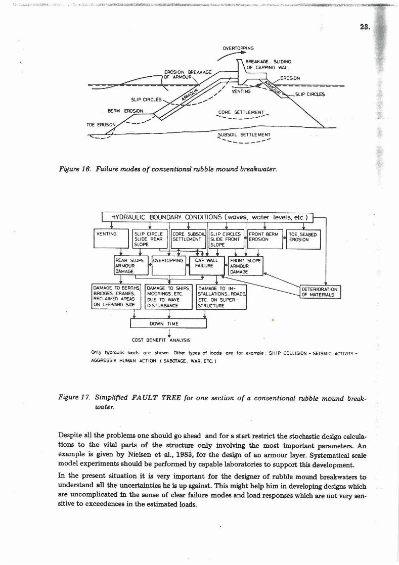
To-day's knowledge makes it of course not very easy to assem the probability functions. This is obvious &om the Figures 16 and 17, which show typical failure modes and the corresponding fault tree. It is seen that not only the distribution functions for a great number qf individual para- meters but also the joint distribution functions for correlated parameters must be estimated.

'speo~ palmqpa aq? tq swuapaaxa o) aA!qy -aas ban qon am pgpi sasuodsar peo~ pw wpom ampj ma13 jo asuas aq? y palmndmo3m am vm* map smdola~ap rr! ca~q d1ar1 iq%ron vu .38als%B dn ? w ~~~~ aw II~ pw?-apm ~1 sra)edhqearq pmom aIqqna JO xaesap aqi ioj qmpodq baas $1 uogutq!s quasad aqq UI

.~namdola~ap g voddns g sauqmoqq alq8d83 Xq parmoj.wd aq ppoqs quaqxadxa lapom ap p!ismapAs 'mXq mom w $0 *sap aq? roj '&961 '.p ia uasIa!N Xq ua~@ aldmxa w .sralarwrsd iwcrodrrr! lsom aw Swlo~rr! Xlno am7an.v ar17 JO slrsd wra aq? o) mo!i -Tap *sap 39s8q3qs aq? la-ax ww 8 IOJ pw pq8 oS ppoqs aao sma~qwd aq? p q~dsaa

3Wll NMW I . t

. . -... &.

LITERATURE

Ahrens, J.R., 1976: Large wave tank teets on rip-rap stability, CERC, No. 61, M a y 1975.

Burcharth, H.F., 1979: The effect of wave grouping on on-shore st~durea. Vol2,1979, pp 189-199. 3

Burchth, H.F., 1981: Full scale dynamic testing of Dolosse to destruction. C h t d Engineering, Vol4, pp 229-251. 5%

Burcharth, H.F., 1983: Material. Structural design of armour unjts. Proc. w a r on Rubble Mound Breakwaters. Royal Institute of Technology. Stockholm, Sweden, 1983.

Burcharth, H.F., 1983: The Way Ahead. Roc. Conference Breakwaters, des* & consbction. Institution of Civil Engineers, London, 1983.

Burcharth, H.F., Thompson, A., 1983: stabili* of Armour Units in Oscilla Flow. Proc. Coa- stal Stru- '83. ASCE. Arlington, V i , U.S.A. 3

Dai, Y.B., Kamel, A.M., 1969: Scale effecttests for rubble mound breakwa . U.S. Army En- gineering Waterways Experiment Station, Vicksbug, Misrisipi, Research Report H-69-2, 1969.

Gravesen, H., Jensen, O.J., Serensen, T., 1979: Stabiity of rubble mound breakwaters 11. h e - sented at Coastal Structures 79, Virginia, U.S.A.

Jensen, O.J., Serensen, T., 1979: OvmpilLing/overtopping of rubble mound breakwaters. Result of studies, useful in design procedures. Coastal Engineering, Vol3,1979.

Jensen 0. J., Kirkegaard, J., 1985: Comparison of hydraulic models of port and marine struc- tures with field measurements. Proc. Int. Conf. on Numerical and Hydreulic Modelling of Ports and Harbours. Birmingham, U.K., 1985.

Le Mehaute, B., Wang, S., 1984: Effects of measurement error on long-term statistics. Proc. 19th - Coastal Eng. Cant, pp 347361, Houston, 1984. -

Lundgren, H., 1969: Wave shock forces: An analysis of deformations and forces in the wave and in the foundation. Roc. Symposium on Research on Wave Action. Delft, The Netherlands 1969.

Nielsen, S.R.K., Burcharth, H.F., 1983: Stochastic design of rubble mound breakwaters. hoc. 11th IFIP Conf. on System Modelling and Optimization, Copenhagen, 1983. Extended version published by Hydra& & Coastal Engineering Laboratmy, Department of Civil Engineering, University of Aalbog, Denmark.

Nielsen, S.R.K., Burcharth, H.F., 1985: On the uncertainties related to estimates on Weibull di- stributed parameters. Note in Danish. Hydraulics and Coastal Engineering Laboratory, Department of Civil Engineering, University of Aalborg, Denmark. '

.Petrauskas, C., Aagaard, P.M., 1971: Extrapolation of historical stom data for estimating design -- -'A wave heights. Journal of Society of Petroleum Engineers, Vol2,1971, pp 25-35. Rosbjerg, D., 1981: Estimation af ekstreme bslgefenomener. Lecture note (in Danish). ISVA.

Technical University of Denmark. Stive, M.J.F., 1985: A scale comparison of waves breaking on a beach. Coastal Engineering, Vol

9,1985, pp 151-158. 1 Thunbo Christensen, F., Broberg, P.C., Sand, S.E., Tryde, P., 1984: Behaviour of rubble mound

breakwater in directional and uni-directional waves. Coastal Engineering, Vol 8,1984, I

pp 265-278. Timco, G.W., 1981: The development, properties and production of strength-reduced model ar-

mom units. NRCIDME report LTR-HY-92. National Research Council, Canada. Timco, G.W., 1983: On the interpretation of rubble mound breakwater testa. Proc. Conf. on the

design, maintenance and performance of coastal structures. ASCE. Vkghh, 1983. Timco, G.W., Mansard, E.P.D., Ploeg, J., 1984: Stability of breakwaters with variations in core

permeab ' i . Proc. 19th International Conference on Coastal Engineering, Houston, Texas, 1984.

Wang. S., Le Mehaute, D., 1983: Duration of measurements and long-term wave statistics. Jour- nal of Waterway, Port, Coastal and Ocean Engineering, ASCE, Vol109, No. 2,1983, pp 236-247.