aberystwyth university exact solution of a nonlinear heat

Aberystwyth University

Exact solution of a nonlinear heat conduction problem in a doubly periodic 2Dcomposite materialKapanadze, D.; Mishuris, G.; Pesetskaya, E.

Published in:Archives of Mechanics

Publication date:2015

Citation for published version (APA):Kapanadze, D., Mishuris, G., & Pesetskaya, E. (2015). Exact solution of a nonlinear heat conduction problem ina doubly periodic 2D composite material. Archives of Mechanics, 67(2), 157-178.

General rightsCopyright and moral rights for the publications made accessible in the Aberystwyth Research Portal (the Institutional Repository) areretained by the authors and/or other copyright owners and it is a condition of accessing publications that users recognise and abide by thelegal requirements associated with these rights.

• Users may download and print one copy of any publication from the Aberystwyth Research Portal for the purpose of private study orresearch. • You may not further distribute the material or use it for any profit-making activity or commercial gain • You may freely distribute the URL identifying the publication in the Aberystwyth Research Portal

Take down policyIf you believe that this document breaches copyright please contact us providing details, and we will remove access to the work immediatelyand investigate your claim.

tel: +44 1970 62 2400email: [email protected]

Download date: 03. Oct. 2019

brought to you by COREView metadata, citation and similar papers at core.ac.uk

provided by Aberystwyth Research Portal

https://core.ac.uk/display/185310225?utm_source=pdf&utm_medium=banner&utm_campaign=pdf-decoration-v1

Arch. Mech., 67, 2, pp. 157–178, Warszawa 2015

Exact solution of a nonlinear heat conduction problem

in a doubly periodic 2D composite material

D. KAPANADZE1), G. MISHURIS2), E. PESETSKAYA1)

1)A. Razmadze Mathematical Institute

Tbilisi State University

Georgia

e-mails: [email protected], [email protected]

2)Aberystwyth University, UK

and

Rzeszów University of Technology, Poland

e-mail: [email protected]

An analytic solution of a stationary heat conduction problem in anunbounded doubly periodic 2D composite whose matrix and inclusions consist ofisotropic temperature-dependent materials is given. Each unit cell of the compositecontains a finite number of circular non-overlapping inclusions. The correspondingnonlinear boundary value problem is reduced to a Laplace equation with nonlinearinterface conditions. In the case when the conductive properties of the inclusionsare proportional to that of the matrix, the problem is transformed into a fully lin-ear boundary value problem for doubly periodic analytic functions. This allows oneto solve the original nonlinear problem and reconstruct temperature and heat fluxthroughout the entire plane. The solution makes it possible to calculate the averageproperties over the unit cell and discuss the effective conductivity of the composite.We compare the outcomes of the present paper with a few results from literature andpresent numerical examples to indicate some peculiarities of the solution.

Key words: nonlinear doubly periodic composite material, conductivity problem,effective properties of the composite.

Copyright c© 2015 by IPPT PAN

1. Introduction

The present paper is devoted to analysis of a steady-state heat conductionproblem in 2D unbounded doubly periodic composite materials with tempera-ture dependent conductivities. Our primary goal is to find an exact solution tothe problem. Then we try to utilize this solution to make some conclusions onthe effective properties of the nonlinear composite. Note that two problems, i.e.,reconstruction of the exact solution (temperature and flux) at each point of thecomposite material and the evaluation of its effective properties, are mutuallyrelated but completely different problems. It is clear that, knowing an exact so-

158 D. Kapanadze, G. Mishuris, E. Pesetskaya

lution for periodic composite, one can provide the standard averaging procedureover the unit cell and thus obtain some estimate for the effective properties ofthe entire composite. On the other hand, having effective properties of a com-posite, one can solve the respective boundary value problem for that averagedmaterial and then compute the respective solution. However this information isnot sufficient to reconstruct the mechanical/physical fields at each specific pointof the original composite.

Moreover, depending on the assumptions made during an averaging process(which effectively means searching for different basic cell solutions), differentapproximate formulae for the effective properties can be delivered. There areseveral justified methods for doing so in the case of linear composite [1]. In thosecases the relation between the two problems (solving the problem for compositeand estimation of its effective properties) are well-developed. Unfortunately, inthe case of composites with components depending on the solution it still remainsa challenging problem. In this paper we deliver not only an exact solution to thespecific nonlinear 2D unbounded doubly periodic composite but also indicatesome open questions related to the evaluation of the effective properties of suchcomposites.

The theory and technique of finding the solution to linear boundary valueproblems for 2D unbounded doubly periodic composite materials with constantconductivities of their components are well-developed. The multipole expansionmethod provides an efficient analysis of properties of different complex heteroge-neous structures (see, for example, [1] where a history of the multipole expansionmethod development is also given in detail). This method is efficient in both 2Dand 3D cases and an arbitrary shape of inclusions. Another method utilisingcomplex analysis techniques and functional equations was proposed in [2] andfurther developed in [3]–[5]. It allows the finding of temperature and flux dis-tributions in composites with an arbitrary number of circular non-overlappinginclusions of different size in the periodicity cell and to determine in an explicitform the effective conductivity of such composite materials. Composites witha rectangular checkerboard structure were analytically investigated using themethods of complex analysis in [6].

General methods to deduce approximate formulae for effective properties ofheterogeneous media were presented in [7] and [8]. Effective properties of ma-terials with complicated macrostructure are usually studied on the basis of theasymptotic homogenization method stated in [9]–[13] and others. Solutions to theproblems with multicracks (which is different in comparison with the inclusions)were discussed in [14]. Important cross-section relationships between elastic andconductive properties of heterogeneous materials were given in [15]. Essentialprogress in obtaining properties of composites has already been achieved utiliz-ing numerical analysis. We refer the prospective reader to the papers (and the

Exact solution of a nonlinear heat conduction problem. . . 159

literature therein) for finite element method (cf. [16], [17]) and boundary elementmethod (cf. [18]).

Problems involving nonlinear heat conduction can be divided into two majorclasses. The first one is when the material parameters depend on the gradient ofthe temperature, and the second one is when the parameters are functions of thetemperature itself. The problems of the first class are close to the problems fornonlinear dielectrics and discussed in the series of works [19]–[25], and others.The respective theory is well-developed.

In contrast, the theory of composite materials with temperature-dependentproperties is still under development. Homogenization theory for random com-posites is studied in [26]. For periodic media, there are several attempts to eval-uate the thermal conductivity of thermo-sensitive heterogeneous materials. Theasymptotic homogenization technique for periodic microstructure with temper-ature independent thermal conductivities is used and extended in [27]. Authorsalso derived Hashin-Shtrikman type bounds for the effective conductivity of cer-tain types of nonlinear composites. In [28] and [29], the authors revisited thehomogenization problem for a nonlinear composite in terms of Padé approxi-mation evaluating the effective conductivity of a square array of densely packedcylinders. Recently, based upon classical approaches, the homogenization pro-cedure for a random composite with conductivities dependent on temperaturein a partial case was developed in [30]. The authors proved that the Eshelbyinclusion approach is not valid when the material parameters are functions oftemperature and explained why problems for nonlinear composite materials fromthe second class are particularly difficult, as this drastically reduces the numberof methods (discussed above for linear case) which researchers could use.

In the present paper, we construct an exact solution for the unbounded dou-bly periodic nonlinear composite under specific assumptions on material prop-erties of the components. Namely, we consider the static thermal conductivityproblem of unbounded 2D anisotropic composite materials with circular non-overlapping inclusions in the square unit periodicity cell geometrically forminga doubly periodic structure. We suppose that each component of the compositeis perfectly embedded in the matrix. Conductivities of the matrix and the in-clusions depend on the temperature. The key assumption is that ratios of thecomponent conductivities are independent of the temperature. The external fluxis assumed to be arbitrarily oriented with respect to the composite symmetry.We determine the temperature and flux distributions and derive the effectiveconductivity of such composites.

The paper is organized as follows. An accurate formulation of the problem isgiven in Section 2. In Section 3, we reduce the given nonlinear boundary valueproblem defined by nonlinear partial differential equations and linear interfaceconditions to an equivalent, generally speaking, nonlinear boundary problem


for Laplace equations with nonlinear interface conditions. Then we formulateconditions for which the transformed problem becomes linear and thus can beeffectively solved using the technique developed by the authors elsewhere. Nu-merical calculations are performed and discussed in Section 5. In this section,we present effective properties of the composite and discuss the obtained re-sults. Comparison of the results for periodic and random composites from [30]is performed in Section 6. The paper is finished by discussions and conclusions.

2. Statement of the problem

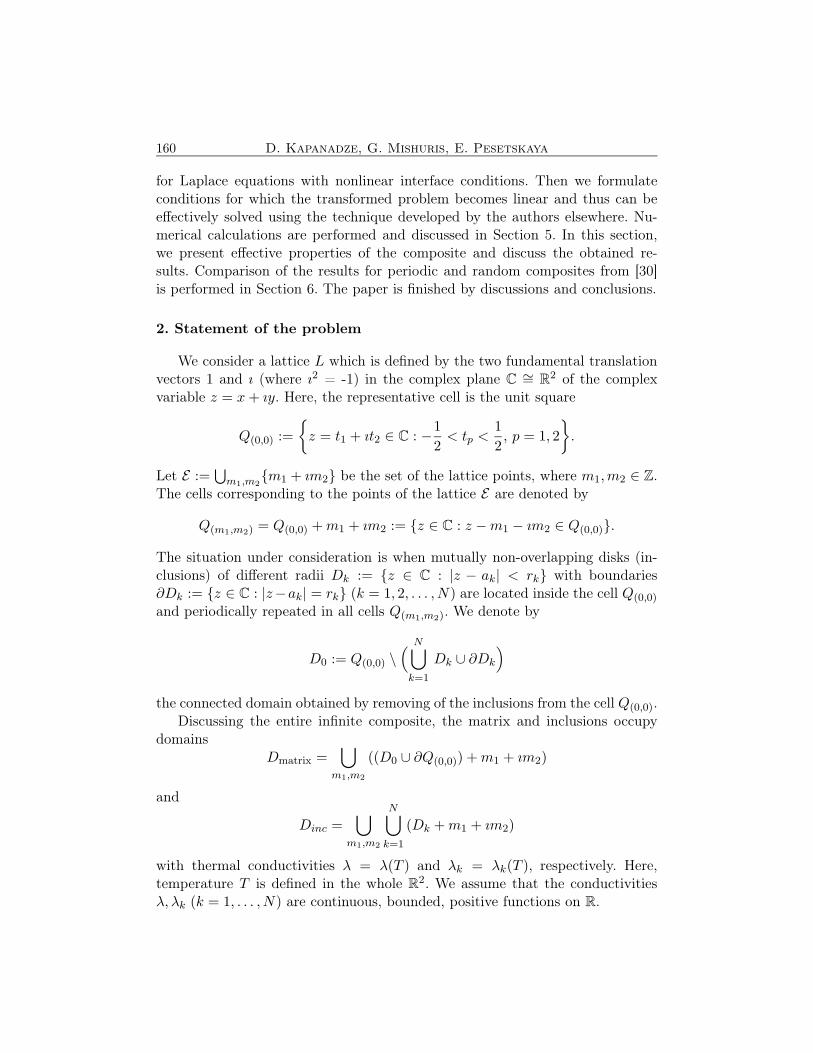
We consider a lattice L which is defined by the two fundamental translationvectors 1 and ı (where ı2 = -1) in the complex plane C ∼= R

2 of the complexvariable z = x + ıy. Here, the representative cell is the unit square

Q(0,0) :=

{

z = t1 + ıt2 ∈ C : −1

2< tp <

1

2, p = 1, 2

}

.

Let E :=⋃

m1,m2{m1 + ım2} be the set of the lattice points, where m1,m2 ∈ Z.

The cells corresponding to the points of the lattice E are denoted by

Q(m1,m2) = Q(0,0) + m1 + ım2 := {z ∈ C : z − m1 − ım2 ∈ Q(0,0)}.

The situation under consideration is when mutually non-overlapping disks (in-clusions) of different radii Dk := {z ∈ C : |z − ak| < rk} with boundaries∂Dk := {z ∈ C : |z−ak| = rk} (k = 1, 2, . . . , N) are located inside the cell Q(0,0)

and periodically repeated in all cells Q(m1,m2). We denote by

D0 := Q(0,0) \(

N⋃

k=1

Dk ∪ ∂Dk

)

the connected domain obtained by removing of the inclusions from the cell Q(0,0).Discussing the entire infinite composite, the matrix and inclusions occupy

domainsDmatrix =

⋃

m1,m2

((D0 ∪ ∂Q(0,0)) + m1 + ım2)

and

Dinc =⋃

m1,m2

N⋃

k=1

(Dk + m1 + ım2)

with thermal conductivities λ = λ(T ) and λk = λk(T ), respectively. Here,temperature T is defined in the whole R2. We assume that the conductivitiesλ, λk (k = 1, . . . , N) are continuous, bounded, positive functions on R.


lm(T) lk(T)

Fig. 1. 2D doubly periodic composite with inclusions.

We search for the steady-state distribution of the temperature and heat fluxwithin such a composite. The problem is equivalent to determining the functionT = T (x, y) satisfying the nonlinear differential equations

∇(λ(T )∇T ) = 0, (x, y) ∈ Dmatrix,(2.1)

∇(λk(T )∇T ) = 0, (x, y) ∈ Dinc.(2.2)

We assume that the perfect (ideal) contact conditions on the boundariesbetween the matrix and inclusions are satisfied:

T (s) = Tk(s), s ∈⋃

m1,m2

(∂Dk + m1 + ım2),(2.3)

λ(T (s))∂T (s)

∂n= λk(Tk(s))

∂Tk(s)

∂n, s ∈

⋃

m1,m2

(∂Dk + m1 + ım2).(2.4)

Here, the vector n is the outward unit normal vector to ∂Dk. According to theformulation, the flux and the temperature are continuous functions throughoutthe entire structure.

We assume that the average flux vector of intensity A is directed at an angleθ to axis Ox (see Fig. 1) which does not coincide, in general, with the orientation


of the periodic cell. This gives the following conditions∫

∂Q(top)(m1,m2)

λ(T )Ty ds = −A sin θ,(2.5)

∫

∂Q(right)(m1,m2)

λ(T )Tx ds = −A cos θ.(2.6)

Note that, in general, the flux is not periodic. However, since there are nosources and sinks in the composite, the energy conservation law dictates

(2.7)

∫

∂Q(m1,m2)

λ(T )∂T

∂nds = 0.

This, in turns, allows us to replace conditions (2.5) and (2.6) with those definedon the opposite sides of the cell.

3. Reformulation of the problem

To solve the problem, we use the Kirchhoff transformation (cf. [31]) andintroduce new continuous functions f and fk (k = 1, . . . , N)

(3.1) f(T ) =

T∫

0

λ(ξ) dξ, fk(T ) =

T∫

0

λk(ξ) dξ.

Then, using representations (3.1) and changing the dependent variables in thefollowing manner:

(3.2) u(x, y) = f(T (x, y)), uk(x, y) = fk(Tk(x, y)),

we transform the original equations (2.1) and (2.2) into the Laplace equations

∆u = 0, (x, y) ∈ Dmatrix,(3.3)

∆uk = 0, (x, y) ∈ Dinc.(3.4)

Note that f and fk are monotonic increasing functions of temperature and,therefore, there exist their inverses f−1 and f−1

k . The contact conditions (2.3)and (2.4) can be rewritten now as follows:

u = Fk(uk), (x, y) ∈⋃

m1,m2

(∂Dk + m1 + ım2),(3.5)

∂u

∂n=

∂uk

∂n, (x, y) ∈

⋃

m1,m2

(∂Dk + m1 + ım2),(3.6)


where the functions

(3.7) Fk(ξ) := f(f−1k (ξ))

are defined for all ξ ∈ R. Note that in general the functions u and uk may havedifferent values on the interface ∂Dk. The derivative of Fk can be computed asfollows:

(3.8) F ′k(ξ) =

f ′(f−1k (ξ))

f ′k(f

−1k (ξ))

=λ(Tk)

λk(Tk),

where ξ = fk(Tk). Now we use the basic assumption of the paper on the nonlinearconduction coefficients

(3.9) λ(T ) = Ckλk(T ).

This property is satisfied for any T ∈ R by some positive real constants Ck.Then, one can immediately conclude that all functions Fk are linear:

(3.10) Fk(ξ) = Dk + Ckξ.

From (3.1) we have f(0) = 0 and fk(0) = 0, and, therefore, Dk = 0. Note that

(3.11)

∫

Γ

∂u

∂nds = 0, Γ ⊂ Dmatrix,

for any closed curve Γ in the matrix. Moreover, since there is no source (sink)inside the composite (neither in the matrix nor in any inclusion), the same con-dition is satisfied for any closed simply connected curve within the inclusion

(3.12)

∫

Γk

∂uk

∂nds = 0, Γk ⊂ Dk.

Finally, the conditions (2.5) and (2.6) transform into the following:∫

∂Q(top)(m1,m2)

uy ds = −A sin θ,(3.13)

∫

∂Q(right)(m1,m2)

ux ds = −A cos θ.(3.14)

Let us introduce inside the inclusions new harmonic functions:

(3.15) uk(x, y) = Ckuk(x, y).


Then the transmission conditions (3.5) and (3.6) become

u = uk, (x, y) ∈⋃

m1,m2

(∂Dk + m1 + ım2),(3.16)

∂u

∂n=

1

Ck

∂uk

∂n, (x, y) ∈

⋃

m1,m2

(∂Dk + m1 + ım2).(3.17)

A new improved algorithm for solving such a linear boundary value problem is de-veloped and described in detail in [5]. We use this approach in our computations.

4. Effective properties of the composite

This section is devoted to evaluation of the effective properties of a nonlin-ear composite. We assume that the effective conductivity tensor Λe depends onaverage temperature 〈T 〉 and is defined in the following way:

(4.1) 〈λ(T )∇T 〉 = Λe(〈T 〉)〈∇T 〉 or Re(〈T 〉)〈λ(T )∇T 〉 = 〈∇T 〉,

where Re = Λ−1e is the effective resistance tensor. A similar definition to (4.1)

has been used in [25]. Here, the operator 〈·〉 is defined as

〈f〉 =

∫∫

Q(m1,m2)

f(x, y) dx dy.

Note that definition (4.1) needs further justification as the question ariseswhether the approach is invariant with respect to the averaging cell. We willdiscuss this issue later during the computations.

We represent all elements involved in (4.1) in terms of a solution u and uk ofthe problem (3.3)–(3.6). For the total flux in the x-direction, we have

(4.2)

∫∫

Q(m1,m2)

λ(T )∂T

∂xdx dy

=

∫∫

D0+m1+ım2

λ(T )∂T

∂xdx dy +

N∑

k=1

∫∫

Dk+m1+ım2

λk(Tk)∂Tk

∂xdx dy

=

∫∫

Q(m1,m2)

(f(T ))x dx dy +

N∑

k=1

∫∫

Dk+m1+ım2

(fk(Tk))x dx dy

=

∫∫

D0+m1+ım2

∂u

∂xdx dy +

N∑

k=1

∫∫

Dk+m1+ım2

∂uk

∂xdx dy.


Using the first Green’s formula and formulas (3.3), (3.4) and (3.6), we obtain∫∫

Q(m1,m2)

λ(T )∂T

∂xdx dy = −A cos θ,

and similarly∫∫

Q(m1,m2)

λ(T )∂T

∂ydx dy = −A sin θ.

Thus, one can write

(4.3) 〈λ(T )∇T 〉 = −A[cos θ, sin θ]⊤.

Note that this relationship is a direct consequence of the absence of sources orsinks inside the composite.

Due to Gauss–Ostrogradsky formula and the boundary condition (2.3), thecomponents of the term 〈∇T 〉 in (4.1) are defined as

∫∫

Q(m1,m2)

∂T

∂xdx dy =

∫∫

D0+m1+ım2

∂T

∂xdx dy +

N∑

k=1

∫∫

Dk+m1+ım2

∂Tk

∂xdx dy

=

∮

∂D0+m1+ım2

T (s) cos(ns, ei) ds +N

∑

k=1

∮

∂Dk+m1+ım2

[Tk(s) − T (s)] cos(nks , ei) ds

=

∮

∂D0+m1+ım2

T (s) cos(ns, ei) ds =

∮

∂D0+m1+ım2

f−1(u(x, y)) cos(ns, ei) ds,

where ns and nks are the outward unit normal vectors to ∂D0 + m1 + ım2 and

∂Dk + m1 + ım2, respectively, and ei is the basis vector. Analogously,∫∫

Q(m1,m2)

∂T

∂ydx dy =

∮

∂D0+m1+ım2

f−1(u(x, y)) cos(ns, ej) ds.

Finally, the average temperature is

〈T 〉 =

∫∫

Q(m1,m2)

T (x, y) dx dy(4.4)

=

∫∫

D0+m1+ım2

f−1(u(x, y)) dx dy +

N∑

k=1

∫∫

Dk+m1+ım2

f−1k (uk(x, y)) dx dy.

It is more convenient to first compute the components of the effective resistancetensor Re from the second formula in (4.1) and then find the effective conduc-tivity tensor Λe = R−1

e .


5. Numerical examples

5.1. Description of the periodic composite

In our computations we consider a composite where four inclusions are sit-uated inside the cell Q(0,0) with the centers (defined in the notations of com-plex variables): a1 = −0.18 + 0.2ı, a2 = 0.33 − 0.34ı, a3 = 0.33 + 0.35ı,a4 = −0.18− 0.2ı. The radii of the inclusions are the same rk = R = 0.145, thusthe volume fraction of the inclusions for such composite is ν = 4πR2 = 0.2642.With such a choice of the positions of the inclusions, one can expect that thecomposite exhibits anisotropic properties and we will observe this fact. Moreover,apart from the fact that the volume fracture is not particularly high, the inclu-sion boundaries are situated very close to each other (the minimal distance 0.02).Thus, the far field approach in defining the effective properties of such compositeis rather problematic.

Fig. 2. Configuration of the unit cell with four inclusions considered in computation.

Further, we suppose that the heat flows in x-direction (θ = 0) with theintensity A = −1. We choose the conductivity of the matrix λ(T ) to be definedin the following form:

(5.1) λ(T ) =

y1, T < x1,

y2 +y1 − y2

x1T, x1 ≤ T ≤ 0,

y2 +y1 − y2

x2T, 0 ≤ T ≤ x2,

y1, T > x2,


where y1, y2 are positive constants, and x1 < x2. We take for the calculationsx1 = −2, x2 = 2, y1 = 4.5, y2 = 13.5, and define the conductivities of the matrixλ from the condition (3.9) with Ck = 0.09 (k = 1, ..., 4). In Fig. 3, we representthe conductivity function λ. The function λk has the identical shape with thepike taking value λk(0) = λ(0)/Ck = 150.

Fig. 3. The function λ.

For computations, we use the algorithm described in [5]. For the chosenconfiguration it guarantees a computational error less than 10−6.

5.2. Evaluation of the effective conductivity tensor

Note that in the linear case temperature is defined up to an arbitrary ad-ditive constant, and this constant is not involved in the determination of theeffective conductivity of a composite material. This is not generally speaking thecase for nonlinear problems, and one needs to clarify how the additive constant,appearing during the stage of solving the auxiliary linear problem (3.3)–(3.14),influences (or not) the computation of the effective conductivity tensor of theequivalent nonlinear composite. Two procedures can be suggested to evaluatethe effective conductivity.

• First, one can solve the auxiliary linear boundary value problem in a dou-bly periodic domain preserving its uniqueness by any appropriately chosencondition (for example, here we impose that the function u = u∗ satisfiesthe condition u∗(0) = 0). Then, to evaluate the properties of the compositematerial, one can compute the average temperature and the effective re-sistivity for each particular unit cell presenting the data as the functionalrelationship Re = Re(〈T 〉).


It is clear from the character of the chosen nonlinearity of the conductivitycoefficients that the domain where the nonlinear behavior manifests itselflies only inside an infinite strip of unknown finite thickness which dependson the flux characteristics: intensity A and angle θ. Thus, it is obvious thatthe effective conductivity tensor demonstrates nonlinear behavior withina finite interval of temperatures, and thus, one does not need to traceall cells. On the other hand, there is still an infinite number of the cellsbelonging to the strip, therefore one can expect that the result of sucha procedure is representative enough to reconstruct a continuous functionusing some smoothing procedure.

• One can suggest also another method for evaluation of the effective proper-ties. Namely, we consider an arbitrary cell in the original domain and builda set of solutions to the auxiliary problem in the form u = u∗ + C, whereC is an arbitrary constant. Then, for every constant C, the componentsof the effective resistance tensor, Re, and the average temperature, 〈T 〉,are functions of the parameter C. Changing the value of C continuouslyfrom −∞ to ∞, one receives the sought for effective conductivity tensor ofthe composite as a continuous function of the average temperature. Natu-rally, for the conductivities of the composite components analyzed in thisexample, the nonlinear character of the relationship will be observed onlywithin the finite interval of the parameter C. It is clear that this proceduredoes not depend on the chosen cell.

Note that the both methods allow one to determine two components of theeffective resistance tensor Re for each of the two orthogonal flux directions. Thusconsidering θ = 0, we define Re[1, j] = Re[1, j](〈T 〉) (j = 1, 2), and choosingθ = π/2 we find Re[2, j] = Re[2, j](〈T 〉). As a result, the entire tensor Re(〈T 〉)is defined.

To check whether and when the two aforementioned procedures are equiv-alent, we use both of them in our computations. The respective componentsof the effective resistance tensor are represented in Figs. 4 and 5. Dots on thecurves correspond to the second approach, while the continuous lines correspondto values computed for consecutive unit cells. These continuous lines were ob-tained by spline interpolation. Discrepancy between the methods is on the level10−5 while the computational accuracy of the solution itself is 10−6. Taking intoaccount the fact that one needs to integrate and interpolate the data to computethe effective properties, the revealed discrepancy can be considered as a perfectevidence that the both methods provide the same result. However, an accuratemathematical proof is still to be delivered.

Note also that due to the chosen functions determining the conductivities,one can expect the effective conductivity to be an even function of the aver-age temperature. This fact could be also taken into account to reconstruct the


Fig. 4. Main diagonal elements of the effective resistance tensor Re (Re[1, 1] and Re[2, 2])computed by each of the proposed methods.

Fig. 5. Components Re[1, 2] and Re[2, 1] of the effective resistance tensor Re computed byeach of the proposed methods.

properties. However, we do not use this argument in this study to eliminateunnecessary assumptions.

Finally, having the effective resistance tensor Re(〈T 〉), we calculate the effec-tive conductivity tensor Λe(〈T 〉) defined in (4.1). The respective results are pre-sented in Figs. 6 and 7, respectively. One can see that the shape of the functionsare quite similar to that of the functions λ(〈T 〉) and λk(〈T 〉) for the compositecomponents. Only some deviations can be observed near the points where thefunctions are not smooth.


Fig. 6. Diagonal components Λe[1, 1], Λe[2, 2] of the effective conductivity tensor Λe.

Fig. 7. Components Λe[1, 2] and Λe[2, 1] of the effective conductivity tensor.

As one can expect from the very beginning, the composite demonstratesanisotropic properties, that is the components on the main diagonals are not thesame in spite of the fact that the components are fully isotropic materials. Thisfollows from the irregular distribution of the inclusions in the cell. Additionally,the main axes of the effective conductivity tensor do not coincide with the initialx, y-axes. As a result, the resulted tensor is not a diagonal one. However, thecorresponding components (anti-diagonal tensor elements) are small and maybe comparable with the accuracy of the computations. This requires additionalverification, which will be carried out later.


In the next section we evaluate known bounds for the effective propertiesof the nonlinear composite in question. At first glance there is not much logicin doing so. Indeed, since we constructed an analytical solution to the nonlinearproblem and then determined the effective conductivity of the composite directly,it looks like there is no need for such estimate. On the other hand, since thequestion “how should the effective properties of such composites be determined”is still opened, we decided to demonstrate how our results fit into the generalframework.

5.3. Hashin–Shtrikman bounds and other estimates

The general estimates for the effective properties have been evaluated fornonlinear composite in [27] and [32]. First, we start with more crude estimates,giving straightforward elementary bounds of the effective conductivity tensor

(5.2) µ1(T )I ≤ Λe(T ) ≤ µ2(T )I,

where I is the unit tensor and

(5.3)µ1(T ) =

(

1 − ν

λ(T )+

ν

λk(T )

)−1

,

µ2(T ) = (1 − ν)λ(T ) + νλk(T ).

Here λ(T ) and λk(T ) are the conductivities of the matrix and the inclusions,while ν is the volume fraction of the inclusions.

Inequalities (5.2) are the Reuss-type and Voigt-type bounds on the effectivecoefficients (see [1], [27]).

Let us recall that the notation A ≥ B used in (5.2) for matrices means thatthe inequality (Ax, x) ≥ (Bx, x) holds true for an arbitrary vector x ∈ R

n (n = 2in our case). In other words, one needs to show that the following inequalitiesare true:

m11(T ) = µ1 − λe11 ≤ 0, m21(T ) = µ2 − λe

11 ≥ 0,(5.4)

m12(T ) = 4(µ1 − λe11)(µ1 − λe

22) − (λe12 + λe

21)2 ≥ 0,(5.5)

m22(T ) = 4(µ2 − λe11)(µ2 − λe

22) − (λe12 + λe

21)2 ≥ 0.(5.6)

In Figs. 8 and 9 we present the graphs of the minors from equalities (5.4)1,(5.5), (5.4)2 and (5.6), respectively. It is clear that the equalities hold true ina strict way.

Now we check feasibility of the Hashin-Shtrikman bounds extended in [27].These estimates are more narrow than the elementary bounds (5.2) and can be


Fig. 8. Verification of the Reuss-type inequality for the effective properties of the nonlinearcomposite from (5.2).

Fig. 9. Verification of the Voigt-type inequality for the effective properties of the nonlinearcomposite from (5.2).

written in our notations (compare with [27]):

(5.7) tr[

(Λe(T ) − λ(T )I)−1]

≤ 1

µ2(T ) − λ(T )+

1

µ1(T ) − λ(T ),

and

(5.8) tr[

(λk(T )I − Λe(T ))−1]

≤ 1

λk(T ) − µ2(T )+

1

λk(T ) − µ1(T ),

where trA = Ajj , (j = 1, 2). The left- and right-hand sides of the inequalities


a) b)

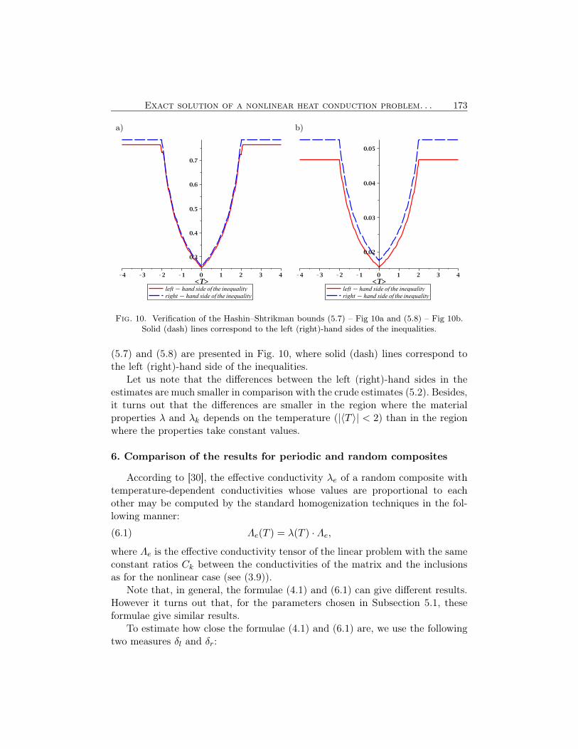
Fig. 10. Verification of the Hashin–Shtrikman bounds (5.7) – Fig 10a and (5.8) – Fig 10b.Solid (dash) lines correspond to the left (right)-hand sides of the inequalities.

(5.7) and (5.8) are presented in Fig. 10, where solid (dash) lines correspond tothe left (right)-hand side of the inequalities.

Let us note that the differences between the left (right)-hand sides in theestimates are much smaller in comparison with the crude estimates (5.2). Besides,it turns out that the differences are smaller in the region where the materialproperties λ and λk depends on the temperature (|〈T 〉| < 2) than in the regionwhere the properties take constant values.

6. Comparison of the results for periodic and random composites

According to [30], the effective conductivity λe of a random composite withtemperature-dependent conductivities whose values are proportional to eachother may be computed by the standard homogenization techniques in the fol-lowing manner:

(6.1) Λe(T ) = λ(T ) · Λe,

where Λe is the effective conductivity tensor of the linear problem with the sameconstant ratios Ck between the conductivities of the matrix and the inclusionsas for the nonlinear case (see (3.9)).

Note that, in general, the formulae (4.1) and (6.1) can give different results.However it turns out that, for the parameters chosen in Subsection 5.1, theseformulae give similar results.

To estimate how close the formulae (4.1) and (6.1) are, we use the followingtwo measures δl and δr:


(6.2)δl = (Λe(T ) − λ(T ) · Λe) · (Λe(T ))−1,

δr = (Λe(T ))−1 · (Λe(T ) − λ(T ) · Λe),

since the tensors given in (4.1) and (6.1) are not co-axial and do not necessarilycommute.

For the composite under consideration, we found with the same accuracy asabove (10−6) the effective conductivity tensor of the linear problem:

(6.3) Λe =

(

1.524131 0.0000270.000027 1.650632

)

.

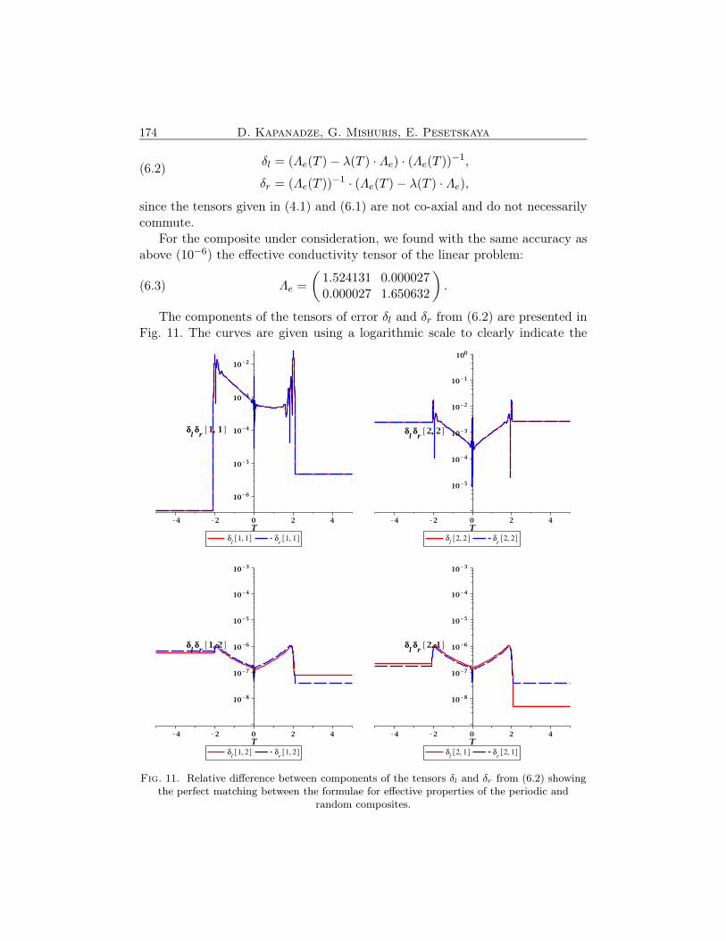
The components of the tensors of error δl and δr from (6.2) are presented inFig. 11. The curves are given using a logarithmic scale to clearly indicate the

Fig. 11. Relative difference between components of the tensors δl and δr from (6.2) showingthe perfect matching between the formulae for effective properties of the periodic and

random composites.


order of component magnitudes. The dash line representees the components of δr

while the solid line corresponds to the components of δl.We note that, although the result obtained in [30] are related to different

types of composite than that analyzed in this paper, our computations showperfect correlation between the models. The largest deviations (near 2%) takeplace near the points where the conductivities of the components as functions oftemperature are not smooth. Moreover, this difference is only observed for thecomponents of the main diagonal of the tensors (6.2). The other two componentsare almost identical (taking into account the computational accuracy). The latterallows us to conclude that the values of the non-diagonal elements (which areon the level of the predicted computational accuracy) have been computed withsufficient accuracy.

Fig. 12. Temperature distribution inside the cell Q(0,0) calculated during utilisation of thesecond method described in the Subsection 5.2. The results correspond to the constants

C = 27 and C = 28, respectively.

Finally, we present in Fig. 12 the distribution of the temperature inside therepresentative cell Q(0,0) calculated during utilisation of the second method todetermine the effective properties described in Subsection 5.2. One can observethat, for the value of constant C = 27, the jump of the temperature along thecell boundaries is not high, and the entire cell lies inside the region where theconductivity exhibits nonconstant behaviour. However, for C = 28, the range ofthe temperature inside the cell lies within the interval when both materials (ma-trix and inclusions) have constant magnitudes, and thus the average propertiescomputed in this case coincide with the respective composite having constantproperties of its constituencies.


7. Discussions and conclusions

As a result of our analysis the following conclusions can be formulated.• An exact solution to the boundary value problem for the unbounded doubly

periodic nonlinear composite, with a special assumption that the compo-nent conductivities are proportional, i.e., their ratios are independent ofthe temperature, can be effectively found by transforming the problem tothe linear one.

• This allows, probably for the first time, the computation of components ofthe effective conductivity tensor in explicit form.

• We show that the average properties of the composite with nonlinear prop-erties satisfy the Reuss-Voigt types and Hashin-Shtrikman estimations.

• We give one example for which we perform numerical calculations andobtain data for the effective conductivity, which allows us to compare for-mulae (4.1) for the effective conductivity tensor for a doubly periodic com-posite and (6.1) derived in [30] for random composites.

We should mention here that the problem of computation of the effectiveproperties of a doubly periodic composite with conductivities depending on tem-perature in its general formulation remains open. It also refers to the accurateproof of the Hashin-Shtrikman estimations (the proof provided in [27] requiresstrong assumptions which cannot be verified directly from the problem formu-lation). We also have not discussed here how the flux intensity may impact onthe results obtained in this paper. At first glance (as it follows from the linearformulation), the flux intensity should not influence the results. On the otherhand, for a high flux intensity the temperature may change dramatically withinone cell, and only a small part of the cell may have the temperature in the rangewhere the conductivities exhibit nonlinear behaviour. All of these problems awaitaccurate analysis.

Acknowledgements

G. Mishuris is grateful for support from the FP7 IRSES Marie Curie grantTAMER No 610547. D. Kapanadze is supported by Shota Rustaveli NationalScience Foundation with the grant number 31/39. E. Pesetskaya is supported byShota Rustaveli National Science Foundation with the grant number 24/03. Theauthors also would like to thank to Prof. S. V. Rogosin for fruitful discussions.

References

1. V. Kushch, Micromechanics of composites: multipole expansion approach, Butterworth-Heinemann, Amsterdam, 2013.

2. V. Mityushev, Zastosowanie równań funkcyjnych do wyznaczania efektywnej przewod-

ności cieplnej materiałów kompozytowych (Application of functional equations to the


effective thermal conductivity of composite materials), WSP Publisher, Słupsk, 1996[in Polish].

3. L. Berlyand, V.V. Mityushev, Generalized Clausius–Mossotti formula for random

composite with circular fibers, J. Statistical Physics, 102, 115–145, 2001.

4. V.V. Mityushev, E.V. Pesetskaya, S.V. Rogosin, Analytical methods for heat con-

duction in composites and porous media, [in:] Cellular and Porous Materials: ThermalProperties Simulation and Prediction. A. Öchsner, G.E. Murch, M.J.S. de Lemos [Eds.],121–164, Wiley, 2008.

5. D. Kapanadze, G. Mishuris, E. Pesetskaya, Improved algorithm for analytical solu-

tion of the heat conduction problem in composites, Complex Variables and Elliptic Equa-tions, 60, 1, 1–23, 2015.

6. R.V. Craster, Y.V. Obnosov, A model four-phase square checkerboard structure, Quar-terly J. Mechanics and Applied Mathematics, 59, 1–27, 2006.

7. G.W. Milton, The Theory of Composites, Cambridge University Press, Cambridge, 2002.

8. M. Kachanov, I. Sevostianov, On quantitative characterization of microstructures and

effective properties, Int. J. Solids and Structures, 42, 309–336, 2005.

9. A. Bensoussan, J.-L. Lions, G. Papanicolaou, Asymptotic Analysis for Periodic

Structures, Elsevier, Amsterdam, 1978.

10. N.S. Bakhvalov, G. Panasenko, Homogenisation: averaging processes in periodic me-

dia, Mathematical Problems in the Mechanics of Composite Materials, Mathematics andIts Applications: Soviet Series, 36, Kluwer Academic Publishers, Dordrecht, 1989.

11. Eh.I. Grigolyuk, L.A. Fil’shtinskij, Periodic Piecewise Homogeneous Elastic Struc-

tures, Nauka, Moscow, 1992 [in Russian].

12. S.K. Kanaun, V.M Levin, Effective field method in mechanics of composite materials,University of Petrozavodsk, 1993.

13. V.V. Jikov, S.M. Kozlov, O.A. Olejnik, Homogenization of Differential Operators

and Integral Functionals, Springer, Berlin, 1994.

14. M. Kachanov, Elastic solid with many cracks and related problems, Advances in AppliedMechanics, 30, 259–445, 1994.

15. I. Sevostianov, M. Kachanov, Connections between elastic and conductive properties

of heterogeneous materials, Advances in Applied Mechanics, 42, 69–253, 2008.

16. L. Greengard, J. Helsing, On the numerical evaluation of the elastostatic fields in

locally isotropic two-dimensional composites, J. Mechanics and Physics of Solids, 43, 1919–1951, 1998.

17. T.I. Zohdi, P. Wriggers, Introduction to Computational Micromechanics, Springer,New York, 2005.

18. P. Fedelinski, R. Gorski, T. Czyz, G. Dziatkiewicz, J. Ptaszny, Analysis of effec-

tive properties of materials by using the boundary element method, Archives of Mechanics,66, 1, 19–35, 2014.

19. P.M. Hui, P. Cheung, Y.R. Kwong, Effective response in nonlinear random compos-

ites, Physica A: Statistical Mechanics and its Applications, 241, 301–309, 1997.


20. P.M. Hui, W.W.V. Wan, Theory of effective response in dilute strongly nonlinear ran-

dom composites, Applied Physics Letters, 69, 1810–1812, 1996.

21. P.M. Hui, Y.F. Woo, W.W.V. Wan, Effective response in random mixtures of linear

and nonlinear conductors, J. Physics-Condensed Matter, 7, L593–L597, 1995.

22. R. Blumendeld, D.J. Bergman, Strongly nonlinear composite dielectrics: A perturba-

tion method for finding the potential-field and bulk effective properties, Physical ReviewB, 44, 7378–7386, 1991.

23. P. De. Ponte-Castaneda, G. Btton, G. Li, Effective properties of nonlinear inho-

mogeneous dielectrics, Physical Review B, 46, 4387–4394, 1992.

24. A. Snarskii, S. Buda, Effective conductivity of nonlinear two-phase media near the

percolation threshold, Physica A, 241, 350–354, 1997.

25. A.A. Snarskii, M. Zhenirovskiy, Effective conductivity of non-linear composites, Phys-ica B, 322, 84–91, 2002.

26. B. Gambin, P. Ponte Castaneda, J.J. Telega, Nonlinear homogenization and its ap-

plications to composites, polycrystals and smart materials. Proc. NATO Adv. Res. Work-shop Math., Phys. and Chem., 170, Springer, Berlin, 2005.

27. A. Galka, J.J. Telega, S. Tokarzewski, Heat equation with temperature-dependent

conductivity coefficients and macroscopic properties of microheterogeneous media, Math-ematical and Computer Modelling, 33, 927–942, 2001.

28. S. Tokarzewski, I. Andrianov, Effective coefficients for real non-linear and fictitious

linear temperature-dependent periodic composites, Int. J. Non-Linear Mechanics, 36, 1,187–195, 2001.

29. S. Tokarzewski, I. Andrianov, V., Danishevsky, G. Starushenko, Analytical con-

tinuation of asymptotic expansion of effective transport coefficients by Padé approximants,Nonlinear Analysis, 47, 2283–2292, 2001.

30. I. Sevostianov, G. Mishuris, Effective thermal conductivity of a composite with thermo-

sensitive constituents and related problems, Int. J. Engineering Science, 80, 124–135, 2014.

31. G.R. Kirchhoff, Theorie der wärme, Leipzig: Druck und Verlag von B.G. Teubner,1894.

32. R.V. Kohn, G.W. Milton, On bounding the effective conductivity of anisotropic com-

posites, [in:] Homogenization and Effective Moduli of Materials and Media, J.L. Ericksen,D. Kinderlehrer, R.V. Kohn and J.-L. Lions [Eds.], Springer, New York, 97–125, 1986.

Received September 9, 2014.

aberystwyth university exact solution of a nonlinear heat

Documents